Algebraic matroids in action

Abstract.

In recent years, various notions of algebraic independence have emerged as a central and unifying theme in a number of areas of applied mathematics, including algebraic statistics and the rigidity theory of bar-and-joint frameworks. In each of these settings the fundamental problem is to determine the extent to which certain unknowns depend algebraically on given data. This has, in turn, led to a resurgence of interest in algebraic matroids, which are the combinatorial formalism for algebraic (in)dependence. We give a self-contained introduction to algebraic matroids together with examples highlighting their potential application.

1. Introduction.

Linear independence is a concept that pervades mathematics and applications, but the corresponding notion of algebraic independence in its various guises is less well studied. As noted in the article of Brylawski and Kelly [6], between the 1930 and 1937 editions of the textbook Moderne Algebra [40], van der Waerden changed his treatment of algebraic independence in a field extension to emphasize how the theory exactly parallels what is true for linear independence in a vector space, showing the influence of Whitney’s [45] introduction of of matroids in the intervening years. Though var der Waerden did not use the language of matroids, his observations are the foundation for the standard definition of an algebraic matroid. In this article, we focus on an equivalent definition in terms of polynomial ideals that is currently useful in applied algebraic geometry, providing explicit proofs for results that seem to be folklore. We highlight computational aspects that tie the 19th century notion of elimination via resultants to the axiomatization of independence from the early 20th century to current applications.

We begin by discussing two examples that will illustrate the scope and applicability of the general theory. Our intention is that they are different enough to illustrate the kinds of connections among disparate areas of active mathematical inquiry that motivated Rota [21] to write in 1986 that “[i]t is as if one were to condense all trends of present day mathematics onto a single finite structure, a feat that anyone would a priori deem impossible, were it not for the mere fact that matroids exist.”

Our first example is an instance of the matrix completion problem in statistics, chosen to be small enough that we can work out the mathematics by hand. In this scenario, a partially filled matrix $M$ of data is given, and a rank $r$ is specified. We seek to understand whether we can fill in (or “complete”) the missing entries so that the resulting matrix has rank $r$. This is related to how interdependent entries of a matrix are.

Example 1.

Suppose that we are given four entries of the following $2\times 3$ matrix:

$$\begin{pmatrix}1&2&*\\ *&6&3\end{pmatrix}.$$

In how many ways can we fill in the missing entries, shown as $*$, if the matrix is to have rank one?

To solve this problem, we let $M=\begin{pmatrix}a&b&c\\ d&e&f\end{pmatrix}$ be a matrix with indeterminates as entries. If the matrix $M$ has rank one, then all $2\times 2$ minors are equal to zero:

$$\begin{array}[]{llllll}(1)&ae-bd=0,&(2)&af-cd=0,&(3)&bf-ce=0.\end{array}$$

Since $b$ and $e$ are nonzero we can solve equations (1) and (3) for $c$ and $d$. We obtain $c=\frac{bf}{e}=1$ and $d=\frac{ae}{b}=3$. Here, Equation (2) is a consequence of the others:

$$af-cd=af-\frac{bf}{e}\frac{ae}{b}=0.$$

Note that if we choose values of $a,b,e,$ and $f$ independently, and our choices are sufficiently generic (in this case, $b$ and $e$ nonzero suffices), we can complete the matrix. However, the values of $c$ and $d$ depend on the four entries that are already specified, and the rank one completion is unique. In the language of algebraic matroids, $\{a,b,e,f\}$ is a maximal independent set of entries in a rank one $2\times 3$ matrix. However, not all subsets of four entries are independent, as the $2\times 2$ minors are algebraic dependence relations. Indeed, if $\{a,b,d,e\}$ are chosen generically, they will not satisfy Equation (1).

A similar setup appears in distance geometry, where the fundamental question is to determine if a list of positive real numbers could represent pairwise distances among a set of $n$ points in $\mathbb{R}^{d}$.

Example 2.

Let $G$ be a graph on vertices $\{1,\ldots,n\}$ with nonnegative edge weights $\ell_{ij}.$ If the $\ell_{ij}$ represent squared distances between points in $\mathbb{R}^{d},$ they must satisfy various inequalities (e.g., they must be nonnegative and satisfy the triangle inequality) as well as polynomial relations.

We examine the simplest case, where $\ell_{12},\ell_{13},\ell_{23}$ are the (squared) pairwise distances between three points. There are no polynomial conditions on the lengths of the edges of a triangle in dimensions $d\geq 2$. However, if the three points lie on a line, then the area of the triangle with these vertices must be zero. The (squared) area of a triangle in terms of its edges is given by the classical Heron formula:

$$A^{2}=s(s-\sqrt{\ell_{12}})(s-\sqrt{\ell_{13}})(s-\sqrt{\ell_{23}}),$$

where $s=\frac{1}{2}(\sqrt{\ell_{12}}+\sqrt{\ell_{13}}+\sqrt{\ell_{23}})$.

The quantity $A^{2}$ may also be computed by taking $\frac{1}{16}\det M_{3}$, where

$$M_{3}=\begin{pmatrix}2\ell_{13}&\ell_{13}+\ell_{23}-\ell_{12}\\ \ell_{13}+\ell_{23}-\ell_{12}&2\ell_{23}\end{pmatrix}.$$

Hence, in dimension $d=1$, the squared edge lengths of a triangle must satisfy the polynomial relation $\det M_{3}=0$. The matrix $M_{3}$ is two times the Gram matrix of pairwise dot products among the vectors ${\bf v}_{1}:={\bf p}_{1}-{\bf p}_{3}$ and ${\bf v}_{2}:={\bf p}_{2}-{\bf p}_{3}$, where the ${\bf p}_{1},{\bf p}_{2},{\bf p}_{3}$ are unknown points in $\mathbb{R}^{d}$, which we can check via the computation

$$\ell_{12}=\|{\bf p}_{1}-{\bf p}_{2}\|^{2}=({\bf v}_{1}-{\bf v}_{2})\cdot({\bf v}_{1}-{\bf v}_{2})={\bf v}_{1}\cdot{\bf v}_{1}+{\bf v}_{2}\cdot{\bf v}_{2}-2{\bf v}_{1}\cdot{\bf v}_{2}=\ell_{13}+\ell_{23}-2{\bf v}_{1}\cdot{\bf v}_{2}$$

This derivation, due to Schoenberg [36] and Young and Householder [46], works for more points (the Gram matrix is $(n-1)\times(n-1)$ for $n$ points) and any dimension (the Gram matrix of point set with $d$-dimensional affine span has rank $d$). A related classical construction, the Cayley–Menger matrix, is due to Menger [30].

What we see is that the polynomial relations constraining squared distances of a $d$-dimensional point set are all derived from the $(d+1)\times(d+1)$ minors of a Gram matrix. These polynomial relations govern how independently the interpoint distances may be chosen. For example, we see that if three points are collinear, then we are free to choose two of the interpoint distances in any way. Once these are chosen, there are (at most) two possibilities for the third.

At their core, the questions that we ask in Examples 1 and 2 are about trying to determine to what extent certain unknown values (distances or matrix entries), are independent of the known ones. Matroids provide a combinatorial abstraction for the study of independence. This perspective was brought to distance geometry by Lovász and Yemini [27]. The point of view there is that the Jacobian of distance constraints defines a linear matroid; by analogy, a similar idea applies to matrix completion in work of Singer and Cucuringu [37].

Recently, work on problems like these has focused on the fact that the matroids appearing are algebraic. In addition to dependent sets we also have the specific polynomials witnessing the dependencies. This aspect of algebraic matroids has been understood for some time, going back to Dress and Lovász in [10], actually exploiting them in applications seems to be newer (see [18, 19, 15]).

Notions of independence abound in other applications as well. For example, chemical reaction networks with mass-action dynamics can be described by a polynomial system of ODE’s. The algebraic properties of these systems at steady state were first exploited by Gatermann [13] and further developed by Craciun, Dickenstein, Shiu and Sturmfels [9]. If a chemist identifies an algebraically dependent set of variables, then she can perform experiments to determine whether the corresponding substances are related experimentally. These dependence relations on subsets, along with their algebraic properties, were used by Gross, Harrington, Rosen and Sturmfels [14] to simplify computations.

Guide to reading

The sequel is structured as follows. We first briefly recall the general definition of a matroid. In the subsequent sections we will discuss three ways of defining algebraic matroids: via a prime ideal, an algebraic variety, or a field extension. Historically, the latter was the standard definition, but the first two are more natural in modern applications. We will see that all three definitions are equivalent, and that there are canonical ways to move between them. We then conclude by revisiting the applications disucssed in the introduction in more detail.

2. Matroids: axiomatizing (in)dependence.

The original definition of a matroid is by Whitney [45], who wanted to simultaneously capture notions of independence in linear algebra and graph theory. The terminology, with “bases” borrowed from linear algebra and “circuits” from graph theory, reflects these origins. It is not surprising that contemporaneous mathematicians such as van der Waerden, Birkhoff, and Maclane were also drawn into this circle of ideas. As Kung writes in [21],

It was natural, in a decade when the axiomatic method was still a fresh idea, to attempt to find the fundamental properties of dependence common to these notions, postulate them as axioms, and derive their common properties from the axioms in a purely axiomatic manner.

We present these axioms in this section.

Definition 3.

A matroid $(E,\mathcal{I})$ is a pair where $E$ is a finite set and $\mathcal{I}\subseteq 2^{E}$ satisfies

1. $\emptyset\in\mathcal{I}$

2. If $I_{2}\subseteq I_{1}\in\mathcal{I}$, then $I_{2}\in\mathcal{I}$.

3. If $I_{1}$ and $I_{2}$ are in $\mathcal{I}$ and $|I_{2}|>|I_{1}|$, there is $x\in I_{2}\setminus I_{1}$ so that $I_{1}\cup\{x\}\in\mathcal{I}$.

The sets $I\in\mathcal{I}$ are called independent.

The complement of $\mathcal{I}$ is denoted $\mathcal{D},$ the dependent sets. The subset $\mathcal{C}\subseteq\mathcal{D}$ of inclusion-wise minimal dependent sets is the set of circuits of the matroid. Finally, $\mathcal{B}\subseteq\mathcal{I}$ of maximal independent sets is the set of bases of $(E,\mathcal{I})$. The bases are all the same size, which is called the rank of the matroid; more generally, the rank of a subset $A\subseteq E$ is the maximum size of an independent subset of $A$.

Intuitively, independence should be preserved by taking subsets, and this gives the motivation for the first two axioms. For the last axiom (augmentation), recall that in linear algebra any linearly independent set of vectors can always be augmented with some vector from a larger linearly independent set without creating a dependence.

As the name suggests, a “matroid” is an abstract version of a matrix, and every matrix gives rise to a matroid. If $M=({\bf x}_{1}\,\cdots\,{\bf x}_{n})$ is an $m\times n$ matrix with columns ${\bf x}_{i}\in\mathbb{R}^{m}$, we define $\mathcal{I}_{M}$ to be the set of all $I\subseteq[n]$ with $\{{\bf x}_{i}\mid i\in I\}$ linearly independent. The reader may check that the axioms are satisfied in Example 4 by inspection and the verification in general is a simple linear algebra exercise.

Example 4.

Let

$$A=\begin{pmatrix}1&1&1&0&0&0\\ 0&0&0&1&1&1\\ 1&0&0&1&0&0\\ 0&1&0&0&1&0\\ 0&0&1&0&0&1\end{pmatrix}.$$

If we label the columns $a,\ldots,f$ from right to left, then we can see that the columns with labels $\{a,b,e,f\}$ form a basis while the columns $\{a,b,d,e\}$ form a circuit. In fact, the column vectors of $A$ all satisfy the same dependencies as the entries of $M$ in Example 1. We will see later that this is not an accident.

It is natural to ask if every matroid arises from a matrix in this way. Whitney posed this question in his foundational paper [45] where he proposed that the matroid on seven elements of the Fano projective plane whose circuits are depicted in Figure 1a was a “matroid with no corresponding matrix.” However, Whitney’s proof does not hold in characteristic 2 and indeed there is a $3\times 7$ matrix with entries in $\mathbb{F}_{2}$ representing this matroid. Whitney was quite aware of this, but in his language, a matrix meant a matrix with complex entries.

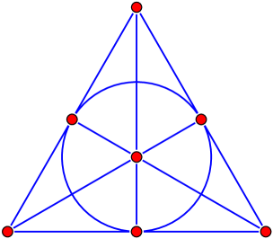
(a)

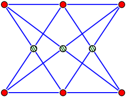
(b)

Figure 1. The Fano and non-Pappus matroids. These are rank $3$ matroids visualized as follows: the elements of the ground set are the points; every set of three points is independent unless there is a curve going through it; no set of four points is independent. The non-Pappus matroid gets its name from the fact that Pappus’s theorem in projective geometry implies that the hatched points in (B) must be collinear, but they are independent in the non-Pappus matroid.

The next year, Mac Lane published a paper [28] attributing to Whitney an example of a rank $3$ matroid on the set $\{1,\ldots,9\}$ whose dependencies are given in Figure 1b. This matroid has become known as the non-Pappus matroid, because (as Mac Lane notes) it forces a violation of Pappus’s theorem. Pappus’s theorem is valid over all fields, so Mac Lane’s example is the first published matroid not representable over any field.

Whitney introduced what he called the “cycle matroid of a graph” [45] which has come to be called a graphic matroid. Given a graph $G=(V,E)$ we define the set $\mathcal{I}_{G}$ to be the subsets of edges that do not contain any circuits. At the heart of the verification that these sets satisfy the axioms in Definition 3 is the fact that all maximal independent sets in a connected component of a graph are spanning trees.

Example 5.

Consider the complete bipartite graph $K_{2,3}$ in Figure 2a and define the matroid $(\{a,b,c,d,e,f\},\mathcal{I}_{K_{2,3}})$. We depict a basis $\{a,b,e,f\}$ in Figure 2b and a circuit $\{a,b,d,e\}$ in Figure 2c. The reader may notice that we again have a set of size six (edges, in this case) whose elements satsify the same dependence relations as in Examples 1 and 4.

(a)

(b)

(c)

Figure 2. A basis and a circuit for the graphic matroid on $K_{2,3}.$

Kung [21, page 18] notes that a “curious feature of matroid theory, not shared by other areas of mathematics is that there are many natural and quite different ways of defining a matroid.” Rota expresses a similar sentiment in his introduction to [21]:

…the unique peculiarity of this field, the exceptional variety of cryptomorphic definitions for a matroid, embarassingly unrelated to each other and exhibiting wholly different mathematical pedigrees.

Indeed, the axioms defining a matroid can be reformulated in terms of bases, rank, dependent sets, or circuits. A number of reference works (e.g., [42, 32, 21]) describe all of these in detail. Since we need them in what follows, we now state the axiomitization of matroids by circuits.

Definition 6.

A matroid is a pair $(E,\mathcal{C})$, where $E$ is a finite set and $\mathcal{C}\subseteq 2^{E}$ satisfies

1. $\emptyset\notin\mathcal{C}$.

2. If $C_{1}\in\mathcal{C}$ and $C_{2}\subsetneq C_{1}$, then $C_{2}\notin\mathcal{C}$.

3. If $C_{1},C_{2}\in\mathcal{C}$, then for any $x\in C_{1}\cap C_{2}$, there is a $C_{3}\in\mathcal{C}$ such that $C_{3}\subseteq(C_{1}\cup C_{2})\setminus\{x\}$.

The sets in $\mathcal{C}$ are the circuits of the matroid.

Here, too, the first two axioms are more intuitive than the third. The third axiom, known as the “circuit elimination axiom,” is natural from the point of view of linear algebra, as two dependence relations in which a vector ${\bf x}$ appears with nonzero coefficient can be combined to get a new dependence relation in which ${\bf x}$ has been eliminated.

3. Matroids via elimination and projection.

The first definition of an algebraic matroid that we will present is formulated in terms of a prime ideal in a polynomial ring. Circuits will be encoded via certain circuit polynomials. To verify that our definition indeed gives a matroid, we establish the circuit elimination axiom using classical elimination theory. Results in the area may be attributed to Bézout in the 18th century and later to Cayley, Sylvester, and Macaulay in the 19th century and early 20th century. Elimination theory fell out of fashion in the mid-twentieth century; Weil [41] wrote that work of Chevalley on extensions of specializations “eliminate[s] from algebraic geometry the last traces of elimination-theory…,” illustrating the attitude of that era. However, computational advances in the last 40 years ignited a resurgence of interest in elimination theory, famously inspiring Abhyankar [1] to write a poem containing the line “Eliminate the eliminators of elimination theory.” We briefly review the relevant results from elimination theory and then define algebraic matroids.

Elimination theory and resultants

We will typically be working with a polynomial ring $k[x_{1},\ldots,x_{r}]$, and our goal will be to eliminate a single variable, say $x_{r},$ from two irreducible polynomials $p(x_{1},\ldots,x_{r})$ and $q(x_{1},\ldots,x_{r})$ by finding polynomials $A(x_{1},\ldots,x_{r})$ and $B(x_{1},\ldots,x_{r})$ so that $Ap+Bq$ is a polynomial in $k[x_{1},\ldots,x_{r-1}]$. For example, we might want to eliminate the variable $d$ in the polynomials $p=ae-bd$ and $q=af-cd$ in Example 1. We see that $cp-bq=ace-bcd-abf+bcd=ace-abf$ is a polynomial combination of $p$ and $q$ not containing $d.$ Now we explain how this kind of elimination can be performed in general.

Let $R$ be an integral domain (typically $R=k[x_{1},\ldots,x_{r-1}]$) and $R[x]$ be the ring of polynomials in $x$ with coefficients in $R$. We denote by $R[x]_{<n}$ the $R$-submodule of polynomials of degree less than $n$ in $x$. With this notation we can define the resultant.

Definition 7 (Sylvester’s resultant).

Let $R$ be an integral domain and let $p$ and $q$ be polynomials of degrees $m$ and $n$ in $R[x]$. The map $(a,b)\mapsto ap+bq$ is an $R$-linear map $R[x]_{<n}\oplus R[x]_{<m}\to R[x]_{<n+m}$. The resultant $\operatorname{Res}(p,q,x)$ is the determinant of this map.

For example, we can perform the previous elimination of $d$ from $ae-bd$ and $af-cd$ by taking the determinant of

$$\begin{pmatrix}-b&-c\\ ae&af\end{pmatrix}.$$

Theorem 8 tells us that if $p$ and $q$ have no common factors, then $\operatorname{Res}(p,q,x)$ is a polynomial combination of $p$ and $q$ in which $x$ has been eliminated. An account of the proof can be found in [8, Section 3.6].

Theorem 8.

The resultant of polynomials $p$ and $q$ in $R[x]$ satisfies the properties:

1. $\operatorname{Res}(p,q,x)\in\langle p,q\rangle\cap R$;

2. $\operatorname{Res}(p,q,x)\equiv 0$ if and only if $p$ and $q$ have a common factor in $R[x]$ of
   positive degree in $x$.

We will apply this theorem to distinct irreducible polynomials in a prime ideal. Since we need some flexibility in terms of which variable to eliminate, we define the support of a polynomial $p\in k[x_{1},\ldots,x_{n}]$ to be the set of variables appearing in it. This next corollary summarizes what we need.

Corollary 9.

Let $k$ be a field, and $P$ be an ideal in $k[x_{1},\ldots,x_{n}]$. If $p$ and $q$ are different irreducible polynomials in $P$ both supported on $x_{n}$, then $0\neq\operatorname{Res}(p,q,x_{n})\in P\cap k[x_{1},\ldots,x_{n-1}]$.

Proof.

Since $p$ and $q$ are irreducible, they don’t have a common factor. Since $p$ and $q$ are in $P$, certainly $\langle p,q\rangle\subseteq P$. Theorem 8 tells us that $0\neq\operatorname{Res}(p,q,x_{n})\in\langle p,q\rangle\cap k[x_{1},\ldots,x_{n-1}]\subseteq P\cap k[x_{1},\ldots,x_{n-1}]$. ∎

Algebraic matroids from prime ideals

Given a set of polynomial equations, we can ask what dependencies they introduce on the variables. If our set of polynomials is a prime ideal, these dependencies satisfy the matroid axioms. The characterization of independent coordinates modulo an ideal in Definition 10 can be deduced from the definition of independence for elements in a field extension, which we give in the next section. We will go in the other direction, giving an elementary proof that seems to be folklore.

Let $k$ be a field, $E=\{x_{1},\ldots,x_{n}\}$ be a set of variables. For any $S\subseteq E$ we define $k[S]$ to be the set of polynomials with variables in $S$ and coefficients in $k$.

Definition 10.

Let $k$ be a field, $E=\{x_{1},\ldots,x_{n}\}$ and $P$ b a prime ideal in $k[E]$. Given $S\subseteq E$, we define

$$\mathcal{I}_{P}=\{S\subseteq E\mid P\cap k[S]=\langle 0\rangle\}$$

to be the set of all subsets of $E$ that are independent modulo $P$. The dependent sets $\mathcal{D}_{P}$ are the subsets of $E$ not in $\mathcal{I}_{P}$.

This notion of independence depends on our choice of coordinates. For example, if $P=\langle x,y\rangle\subseteq k[x,y,z]$, then $\mathcal{I}_{P}$ contains a single maximal independent set, $\{z\}$. However, the ideal $Q=\langle x+2y+3z,x+5y+2z\rangle$, which can be obtained from $P$ via a linear change of coordinates has three maximal independent sets, $\{x\},\{y\},$ and $\{z\}$. It is also the case that very different ideals can give rise to the same independent sets. For example, if $T=\langle x^{2}-y,xy-z\rangle$, then the maximal independent sets of $\mathcal{I}_{T}$ are $\{x\},\{y\},$ and $\{z\},$ which are the same as in those in $\mathcal{I}_{Q}$.

We now show that the elements of $\mathcal{I}_{P}$ are the independent sets of a matroid. First we will show that every minimal dependent set $C$ is encoded by an irreducible polynomial $f_{C}$ that is unique up to scalar multiple.

Theorem 11.

Let $k$ be a field and $P$ a prime ideal in $k[x_{1},\ldots,x_{n}]$. Let $C\subseteq E$. If $P\cap k[C]\neq\langle 0\rangle$ and $P\cap k[C^{\prime}]=\langle 0\rangle$ for all $C^{\prime}\subsetneq C$, then $P\cap k[C]$ is principal and generated by an irreducible polynomial $f_{C}$. The support of $f_{C}$ is all of $C$.

Proof.

First suppose that $f\in P\cap k[C]$ is a nonzero polynomial. Since $k[S]$ is a unique factorization domain, $f$ is a product of irreducible factors $f_{1}\cdots f_{k}$. Because $P$ is prime, at least one of the $f_{i}$ is in $P$. Thus, every $f\in P\cap k[C]$ has an irreducible factor in $P$.

By the minimality hypothesis on $C$, any polynomial $g$ in $P\cap k[C]$ is supported on all of $C$. In particular, if $g$ and $h$ are both in $P\cap k[C]$, they must be supported on a common variable, $x_{i}\in C$. When $g$ and $h$ are irreducible, we then have the situation of Corollary 9. If $g\neq h$, this implies that $P\cap k[C\setminus\{x_{i}\}]\neq\langle 0\rangle$.

Using the line of reasoning above, if $f_{i}$ and $f_{j}$ are distinct irreducible factors of $f$ in $P\cap k[C]$, then we can eliminate a variable in common to them, contradicting the minimality of $C.$ Therefore, we conclude that $f$ is divisible by a unique irreducible factor in $P\cap k[C],$ which we denote by $f_{C}.$ Again, by the minimality of $C$, we can see that $f_{C}$ must be the unique irreducible polynomial in $P\cap k[C],$ and that it divides every polynomial in $P\cap k[C].$ ∎

The polynomial $f_{C}$ appearing in the conclusion of Theorem 11 is called the circuit polynomial of the circuit $C$ in $(E,\mathcal{I}_{P})$. This notion first appears in the paper of Dress and Lovász [10]. It was later explored, in a statistical context, by Király and Theran [18]. The unpublished preprint of Király, Rosen, and Theran [20], where this use of the term “circuit polynomial” originates, studies how symmetries of an algebraic matroid are reflected in the associated circuit polynomials.

Now we are ready show that the sets in Definition 10 are the independent sets of a matroid. Instead of checking the independent set axioms directly, we use the circuit axioms.

Theorem 12.

The pair $(E,\mathcal{I}_{P})$ from Definition 10 is a matroid.

Proof.

With respect to $\mathcal{I}_{P}$, the dependent subsets are those sets $S$ for which $P\cap k[S]\neq\langle 0\rangle$. We define $\mathcal{C}_{P}$ to be the dependent subsets of $E$ that are minimal with respect to inclusion. The result will follow once we have checked the circuit axioms from Definition 6.

Certainly $P\cap k[\emptyset]$ is the zero ideal, which implies that $\emptyset\notin\mathcal{C}_{P}$, which is axiom (1). Minimality of the circuits gives axiom (2) by definition. For use later, we note that if $P\cap k[D]\neq\langle 0\rangle$ then some subset of $D$ is a circuit by axiom (1).

The interesting axiom is (3). Suppose that $C_{1}$ and $C_{2}$ are circuits in $\mathcal{C}_{P}$ with $x_{i}\in C_{1}\cap C_{2}$. By Theorem 11, there are distinct irreducible polynomials $f_{C_{1}}$ and $f_{C_{2}}$ both supported on $x_{i}$ in $P\cap k[C_{1}\cup C_{2}]$. Corollary 9 then implies that there exists a nonzero $h\in P\cap k[(C_{1}\cup C_{2})\setminus\{x_{i}\}]$. Since the support of $h$ is contained in $(C_{1}\cup C_{2})\setminus\{x_{i}\}$, $P\cap k[(C_{1}\cup C_{2})\setminus\{x_{i}\}]\neq\langle 0\rangle$. By the observation above, we have axiom (3). ∎

Every linear matroid is algebraic, though not all algebraic matroids are linear. To see that a linear matroid is algebraic, suppose we are given a matroid on the columns of a $d\times n$ matrix $M$. Let $B=({\bf b}_{1}\,\cdots\,{\bf b}_{r})$ be a matrix whose columns form a basis for the kernel of $M$. We’ll use the vectors ${\bf b}_{i}$ to define an ideal generated by linear forms in the ring $k[x_{1},\ldots,x_{n}].$ Define linear forms $L_{1},\ldots,L_{r}$ by setting $L_{i}={\bf b}_{i}\cdot(x_{1},\ldots,x_{n}).$ An ideal generated by linear forms must be prime, so $P=\langle L_{1},\ldots,L_{r}\rangle$ defines a matroid $\mathcal{I}_{P},$ where the linear forms defining dependent sets of variables exactly record the dependencies among the columns of $M.$

Varieties and projections

We will construct a geometric counterpart to coordinate matroids, using projections of varieties, which we briefly introduce.

Let $k$ be a field and $f_{1},\ldots,f_{m}$ be polynomials in $k[x_{1},\ldots,x_{n}].$ The common vanishing locus of these polynomials is the algebraic set

$$V=V(f_{1},\ldots,f_{m})=\{{\bf p}\in k^{n}\mid f_{1}({\bf p})=\cdots=f_{m}({\bf p})=0\}.$$

In the Zariski topology on $k^{n}$ a set is closed if and only if it is an algebraic set. The Zariski closure, denoted $\overline{X}$, of a subset $X\subseteq k^{n}$ is the smallest algebraic set containing $X$. An algebraic set is called irreducible if it is not union of two nonempty algebraic sets, and we call an irreducible algebraic set a variety. For example, the three equations $ae-bd=0,af-cd=0,$ and $bf-ce=0$ in Example 1 define a variety in $k^{6}$ whose points correspond to $2\times 3$ matrices with rank at most one.

Although we have defined an algebraic set as the solution set of a finite system of polynomial equations, it is not hard to check that if $I=\langle f_{1},\ldots,f_{m}\rangle$ is the ideal generated by the polynomials $f_{i}$, then $V(f_{1},\ldots,f_{m})=V(I).$ Conversely, given an algebraic set $V\subseteq k^{n},$ one may define

$$I(V)=\{f\in k[x_{1},\ldots,x_{n}]\mid f({\bf p})=0\ \forall{\bf p}\in V\},$$

the ideal of all polynomials that vanish on $V.$

What is the relationship between an algebraic set and its vanishing ideal? If $V=V(f_{1},\ldots,f_{m})\subseteq k^{n}$ is algebraic, then $V(I(V))=V$. Since $\{f_{1},\ldots f_{n}\}\subseteq I(V)$, $V(I(V))\subseteq V$. By definition, every $f\in I(V)$ vanishes on $V$, so $V\subseteq V(I(V))$. Starting from an ideal $I\subseteq k[x_{1},\ldots,x_{n}]$, we don’t necessarily have $I(V(I))=I$. For example, if $k=\mathbb{R}$ and $I=\langle x^{2}+y^{2}+1\rangle,$ then $V(I)=\emptyset,$ so $I(V(I))=\langle 0\rangle.$ However, over an algebraically closed field, Hilbert’s famous Nullstellensatz says that $I(V(I))=I$ holds if $I$ is a radical ideal. In this setting, the fundamental “algebra-geometry dictionary” (see, e.g., [8, chapter 4]) says that there is a bijection $V\mapsto I(V)$ between irreducible varieties in $k^{n}$ and prime ideals in $k[x_{1},\ldots,x_{n}]$.

Now that we have a geometric counterpart to prime ideals when $k$ is closed, we need an analogue for elimination. For $S\subseteq\{1,\ldots,n\}$ define a projection $\pi_{S}:k^{n}\to k^{|S|}$ by $\pi_{S}(p_{1},\ldots,p_{n})=(p_{i}\mid i\in S),$ where we preserve the order of the coordinates. We are going to be comparing two kinds of objects, so we take $E=\{1,\ldots,n\}$ as the common ground set that indexes both variables and standard basis vectors of $k^{n}$. For $S\subseteq E$, extend the notation $k[S]$ to means $k[x_{i}:i\in S]$.

If $V\subseteq k^{n}$ is algebraic, then $\pi_{S}(V)$ corresponds to eliminating the variables not in $S$ from its vanishing ideal $I\subseteq k[x_{1},\ldots,x_{n}]$. Suppose that $f\in I\cap k[S]$ and ${\bf p}\in V$. Certainly $f({\bf p})=0$; more interestingly, since $f$ only sees variables in $S$, $f(\pi_{S}({\bf p}))=0$ as well. Hence $\pi_{S}(V)\subseteq V(I\cap k[S])$; since $V(I\cap k[S])$ is closed, it contains $\overline{\pi_{S}(V)}$ as well. When $k$ is closed and $V$ is irreducible, we can get more. This affine version of the “closure theorem” is a key technical tool for us.

Theorem 13.

Let $k$ be an algebraically closed field, and let $V\subseteq k^{n}$ be an irreducible algebraic set with ideal $I=I(V)\subseteq k[x_{1},\ldots,x_{n}]$. Then for all $S\subseteq E$:

1. $\overline{\pi_{S}(V)}$ is irreducible;

2. $I(\overline{\pi_{S}(V)})=I\cap k[S]$.

Proof.

Since $V$ is irreducible, $I$ is prime, which implies that $I\cap k[S]$ is also prime. By [8, Theorem 3.2.3], $V(I\cap k[S])=\overline{\pi_{S}(V)}$, which shows that $\overline{\pi_{S}(V)}$ is irreducible, and (2) follows by the Nullstellensatz. ∎

To make this theorem work, taking the Zariski closure of the image was essential. For instance, we noted that the set $S=\{a,b,e,f\}$ is independent in Example 1. However, if $V=V(ae-bd,af-cd,bf-ce)$, the projection $\pi_{S}:V\to k^{4}$ cannot be surjective because a point with $a=1,b=0,e=1,f=1$ cannot come from a rank one matrix because if $b=0$ the equation $ae-bd=0$ implies that either $a$ or $e$ is zero.

Now we define a geometric analogue of coordinate matroids.

Definition 14.

Let $k$ be an algebraically closed field and let $V\subseteq k^{n}$ be an irreducible variety. Define

$$\mathcal{I}_{V}=\{S\subseteq E\mid\overline{\pi_{S}(V)}=k^{|S|}\}.$$

To check that we have defined a matroid, instead of verifying the axioms, we will use the relationship between projection and elimination to relate $\mathcal{I}_{V}$ to a coordinate matroid.

Theorem 15.

The set $\mathcal{I}_{V}$ from Definition 14 gives the independent sets of a matroid on $E$. We call this the basis projection matroid.

Proof.

Let $P$ be the vanishing ideal of $V$. Since $k$ is closed, the algebra-geometry dictionary tells us that $P$ is prime. Hence the coordinate matroid $(\{1,\ldots,n\},\mathcal{I}_{P})$ is defined. The set $\mathcal{I}_{V}$ is the same as $\mathcal{I}_{P}$, since,

$$S\in\mathcal{I}_{V}\Longleftrightarrow\overline{\pi_{S}(V)}=k^{|S|}\overset{\text{Thm. \ref{thm: closure}}}{\Longleftrightarrow}P\cap k[S]=\langle 0\rangle\Longleftrightarrow S\in\mathcal{I}_{P}.$$

Hence $(E,\mathcal{I}_{V})$ is a matroid. ∎

The advantage of basis projection matroids is that sometimes it is more convenient to think geometrically. In Example 2, the fibers of the projection map contain useful geometric information. For a fixed $G\subseteq\binom{n}{2}$, if $\ell_{G}$ is the vector $(\ell_{ij}:ij\in G)$, then the fiber $\pi_{G}^{-1}(\ell_{G})$ tells us about the achievable distances between pairs of points outside of $G$, a perspective emplyoed by Borcea [4], Borcea and Streinu [5], and Sitharam and Gao [38]. Similarly, in Example 1, the fibers of the projection map are the “completions” of a low-rank matrix from the observed entries.

4. Algebraic matroids and field theory.

Classically, algebraic matroids are defined in terms of field extensions. Let $k$ be a field and $K\supset k$ a field extension. We say that $S=\{\alpha_{1},\ldots,\alpha_{n}\}\in K$ are algebraically dependent over $k$ if there exists a nonzero polynomial $f\in k[x_{1},\ldots,x_{n}]$ with $f(\alpha_{1},\ldots,\alpha_{n})=0.$ If no such polynomial exists we say the elements are algebraically independent over $k$.

Definition 16.

Let $K\supset k$ be an extension of fields and $E=\{\alpha_{1},\ldots,\alpha_{n}\}$ be a subset of $K\backslash k.$ Without loss of generality, we assume that $K=k(E)$. We define a matroid $(E,\mathcal{I}_{K})$ with ground set $E$ and define $S\subseteq E$ to be an independent set if $S$ is algebraically independent over $k$.

The classical definition is equivalent to the ones in terms of ideals and varieties. If $k\subseteq E=\{\alpha_{1},\ldots,\alpha_{r}\}\subseteq K$, and we define $\varphi:k[x_{1},\ldots,x_{r}]\to k[\alpha_{1},\ldots,\alpha_{r}]$ by $\varphi(x_{i})=\alpha_{i},$ then $P=\ker\varphi$. The independent sets of the coordinate matroid $(\{x_{1},\ldots,x_{n}\},\mathcal{I}_{\ker\varphi})$ correspond naturally to independent subsets of $(E,\mathcal{I}_{K})$. Moreover, this construction can be reversed. If we start with a prime ideal $P$, $k[\{x_{1},\ldots,x_{n}\}]/P$, is an integral domain. Hence its field of fractions $K\supset k$ is defined. Defining $\{\alpha_{1},\ldots,\alpha_{n}\}$ as the elements of $K$ corresponding to the $x_{i}$ produces an algebraic matroid $(E,\mathcal{I}_{K})$ with independent sets corresponding to those in $(\{x_{1},\ldots,x_{n}\},\mathcal{I}_{P})$. We saw that there is a natural correspondence between basis projection matroids and coordinate matroids if $k$ is algebraically closed in Theorem 15.

We are now in possession of three different-looking, as Rota puts it “cryptomorphic”, definitions of an algebraic matroid. As an illustration of why this is useful, we consider the rank, which is an important quantity in almost any application. The rank of an algebraic matroid $(E,\mathcal{I}_{K})$ is the transcendence degree of $K$ over $k$. Via the correspondences above, we can also see that this gives the rank for the associated coordinate and basis projection matroids. Does the rank of a coordinate matroid $(E,\mathcal{I}_{P})$ or a basis projection matroid $(E,\mathcal{I}_{V})$ have any meaning? The answer is yes, they are the dimensions of $k[E]/P$ and $V$, respectively. This is difficult to see directly, even with the (somewhat technical, see, [11, Chapter 8]) definitions of dimension for ideals and varieties. However, both quantities are known to be equal to the transcendence degree of the extension we constructed to go between $(E,\mathcal{I}_{P})$ and $(E,\mathcal{I}_{K})$.

In the case of field extensions the theory follows from work of van der Waerden who showed that “[t]he algebraic dependence relation has the following fundamental properties which are completely analogous to the fundamental properties of linear dependence,” [40, Ch. VIII, S. 64]. The connection was also known to Mac Lane, who wrote about lattices of subfields in [28] and drew attention to “connection[s] to the matroids of Whitney” and the “lattices by Birkhoff.”

It seems that algebraic matroids were largely forgotten after Mac Lane until the work of Ingleton in the 1970s. Ingleton asked the basic question for algebraic matroids that Whitney had already considered in the 1903’s for linear representability: is every matroid realizable as an algebraic matroid? This was answered by Ingleton and Main [17] in the negative who showed that the Vámos matroid, displayed in Figure 3, is not algebraic.

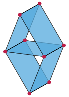
Figure 3. The Vamos matroid. This is a rank $4$ matroid, shown according to the convention that all sets of size at most $4$ are independent, except for the size $4$ sets indicated by shaded quadrilaterals. Picture from [12].

What about the relationship between algebraic and linear matroids? In characteristic zero, the two classes are the same.

Theorem 17 (Ingleton [16]).

If a matroid is realizable as an algebraic matroid over a field $k$ of characteristic zero, then it is also realizable as a linear matroid over $k$.

What about fields of positive characteristic? Whitney’s example of a matroid that is not linearly representable over $\mathbb{C}$ but is over $\mathbb{F}_{2}$ shows that the characteristic of the underlying field matters. The characteristic of the field also makes a big difference in determining algebraic representability. In a series of papers in the 1980s Bernt Lindström [23, 24, 25, 26] demonstrated that there are infinitely many algebraic matroids representable over every characteristic besides zero, and not linearly representable over any field. Characterizing which matroids are algebraic (in positive characteristic) is an active area of research, including the recent advances of Bollen, Draisma and Pendavingh [3] (see also Cartwight [7]).

5. Applications.

We revisit the earlier examples, including matrix completion, rigidity theory, and graphical matroids, from the point of view of algebraic matroids, highlighting the connections revealed by the common language.

A matrix, an ideal, and a variety

An $m\times n$ matrix $A=({\bf a}_{1}\,\cdots\,{\bf a}_{n})$ with ${\bf a}_{i}\in\mathbb{Z}^{m}$ gives rise to a matroid that can be realized as a linear matroid and a coordinate matroid in a natural way via the construction of the toric variety $X_{A}$ associated to $A$. (Of course, once we have the coordinate matroid we also have the basis matroid and the algebraic matroid of the field of fractions of the coordinate ring of $X_{A}.$)

From the data of $A$ we get a map $\varphi_{A}:(\mathbb{C}^{*})^{m}\to\mathbb{C}^{n}$ given by $\varphi_{A}({\bf t})=({\bf t}^{{\bf a}_{1}},\ldots,{\bf t}^{{\bf a}_{n}}),$ where ${\bf t}^{{\bf a}}=t_{1}^{a_{1}}\cdots t_{m}^{a_{m}}$. As shown in [39], the variety $X_{A}$ defined to be the Zariski closure of the image of $\varphi_{A}$ has ideal $I_{A}=\langle{\bf x}^{{\bf u}}-{\bf x}^{{\bf v}}\mid{\bf u},{\bf v}\in\mathbb{Z}_{\geq 0},{\bf u}-{\bf v}\in\ker A\rangle.$ Since elements of $\ker A$ are dependence relations on the columns of $A$, we see that the linear matroid on the columns of $A$ is the same as the algebraic matroid defined by the ideal $I_{A}.$ The variety $X_{A}$ is called a toric variety as it contains the torus $(\mathbb{C}^{*})^{m}$ as a dense open subset.

Returning to Example 4, we see that the columns of

$$A=\begin{pmatrix}1&1&1&0&0&0\\ 0&0&0&1&1&1\\ 1&0&0&1&0&0\\ 0&1&0&0&1&0\\ 0&0&1&0&0&1\end{pmatrix}$$

define a parameterization $\varphi_{A}({\bf t})=(t_{1}t_{3},t_{1}t_{4},t_{1}t_{5},t_{2}t_{3},t_{2}t_{4},t_{3}t_{5}).$ If we give the target space coordinates $a,\ldots,f,$ then $(1,0,0,1,0)-(0,1,0,1,0,0)\in\ker A$, and this tells us that the polynomial $ae-bd$ is in $I_{A}.$ (Indeed, if we let $\psi=ae-bd,$ then $\psi(\varphi({\bf t}))=(t_{1}t_{3})(t_{2}t_{4})-(t_{1}t_{4})(t_{2}t_{3})=0.$)

So, the linear dependence relations on the columns of $A$ give algebraic dependence relations on $a,\ldots,f.$ This is true for any general toric variety $X_{A}$ that arises from an integer matrix $A$ in this way. For more detail on how the circuits of the matroid on the columns of $A$ are related to the ideal $I_{A}$, see [39, chapter 4]. We will soon see that the matrix in Example 4 has a special form that provides a connection to the rank one matrix completion problem.

Matrix completion, varieties, and bipartite graphs

Algebraic matroids were used to study the matrix completion problem by Király, Theran, and Tomioka [19]. We now provide a brief introduction.

Define $I_{m\times n,r}$ to be the ideal generated by the $(r+1)\times(r+1)$ minors of the generic matrix $M=({\bf x}_{1}\,\cdots\,{\bf x}_{n})$ where ${\bf x}_{i}$ is a column vector of $m$ indeterminates. This ideal is prime, so defines an algebraic matroid, $\mathcal{M}_{I_{m\times n,r}}=(\{(1,1),\ldots,(m,n)\},\mathcal{I}_{I_{m\times n,r}})$. This is the matroid on the entries of a general $m\times n$ matrix of rank $r.$

Theorem 18.

The rank of $\mathcal{M}_{I_{m\times n,r}}$ is $r(m+n-r)$.

Proof sketch.

The dimension of the variety $V_{m\times n,r}$ of $m\times n$ matrices of rank at most $r$ is $r(m+n-r)$. One intuition for this, which isn’t far from a proof, is that you can specify the first $r$ rows and columns of the matrix freely and then rest of the matrix is determined. This process sets $rm+rn-r^{2}$ entries in total. ∎

Why are the elements of $I_{2\times 3,1}$ the same as the polynomials that vanish on the toric variety $X_{A}$ discussed above? Observe that the coordinates of $\varphi_{A}({\bf t})=(t_{1}t_{3},t_{1}t_{4},t_{1}t_{5},t_{2}t_{3},t_{2}t_{4},t_{3}t_{5})$ can be rearranged into a matrix:

$$\begin{pmatrix}t_{1}\\ t_{2}\end{pmatrix}\begin{pmatrix}t_{3}&t_{4}&t_{5}\end{pmatrix}=\begin{pmatrix}t_{1}t_{3}&t_{1}t_{4}&t_{1}t_{5}\\ t_{2}t_{3}&t_{2}t_{4}&t_{2}t_{5}\end{pmatrix}.$$

Replacing each product with a distinct variable, we have the matrix of indeterminates from Example 1:

$$M=\begin{pmatrix}a&b&c\\ d&e&f\end{pmatrix}.$$

The $2\times 2$ minors of $M$ are polynomials that vanish on the multiplication table by commutativity and associativity:

$$ae-bd=(t_{1}t_{3})(t_{2}t_{4})-(t_{1}t_{4})(t_{2}t_{3})=t_{1}t_{2}t_{3}t_{4}-t_{1}t_{2}t_{3}t_{4}=0.$$

More generally, any $m\times n$ matrix with distinct variables as entries can be interpreted as the formal multiplication table of sets of size $m$ and $n$, respectively. The $2\times 2$ minors will vanish on the variety parameterized by these products, the classical Segre variety $\mathbb{P}^{m-1}\times\mathbb{P}^{n-1}.$

The combinatorics of the circuits in Example 1 can also be encoded in the bipartite graph $K_{2,3}$ with vertices labeled $t_{1},\ldots,t_{5}$ so that each edge corresponds to a product $t_{i}t_{j}$, as shown in Figure 4. Each 4-cycle in this graph corresponds to a $2\times 2$ minor, and these are exactly the circuits of the matroid. The maximal independent sets are

$$\begin{array}[]{llllll}\{a,b,c,d\},&\{a,b,c,e\},&\{a,b,c,f\},&\{a,d,e,f\},&\{b,d,e,f\},&\{c,d,e,f\},\\ \{a,b,e,f\},&\{a,c,f,e\},&\{a,b,d,f\},&\{b,c,d,f\},&\{a,c,d,e\},&\text{ and }\{b,c,d,e\}.\end{array}$$

Given (generic) values for the entries in any of these sets there is a unique matrix completion, because the circuit polynomials are all linear in the missing entry.

Figure 4. $K_{2,3}$.

Distance geometry and rigidity theory

Given $n$ points ${\bf x}_{1},\ldots,{\bf x}_{n}\in\mathbb{R}^{d},$ there are $\binom{n}{2}$ equations $({\bf x}_{i}-{\bf x}_{j})\cdot({\bf x}_{i}-{\bf x}_{j})=\ell_{ij}$ giving the squared distances between pairs of points. The (closure of) the image of the squared length map $({\bf x}_{1},\ldots,{\bf x}_{n})\mapsto(({\bf x}_{i}-{\bf x}_{j})\cdot({\bf x}_{i}-{\bf x}_{j}))$ is a variety $\mathrm{CM}_{d,n}$ in $\mathbb{R}^{\binom{n}{2}}$ with defining ideal $I_{d,n}$ given by the $(d+1)\times(d+1)$ minors of the $(n-1)\times(n-1)$ Gram matrix $M_{d,n}$ with $ij$ entry equal to

$$\begin{cases}2\ell_{in}&\text{if $i=j$}\\ \ell_{in}+\ell_{jn}-\ell_{ij}&\text{if $i\neq j$}\end{cases}.$$

It follows from work of Whiteley [44] and Saliola and Whiteley [35], that $I_{n,d}$ has a matroid isomorphic to the one associated with the ideal of the $(d+2)\times(d+2)$ minors of a generic symmetric $n\times n$ matrix, modulo its diagonal. This was independently rediscovered by Gross and Sullivant [15].

It is interesting to ask which interpoint distances are needed in order to determine the rest, generically. This is related to the central question in the theory of the rigidity of bar and joint frameworks. To formalize this, we may fix a graph $G$ on $n$ vertices and think of the edges as fixed-length bars and the vertices as universal joints. A realization of $G$ in $\mathbb{R}^{d}$ is a bar-and-joint framework. A graph $G$ has a flexible realization if the fiber of $\pi_{G}:\mathrm{CM}_{d,n}\to\mathbb{R}^{|G|}$ has positive dimension.

If $d=2$, i.e. we are examining bar-and-joint frameworks in the plane, then the rank of the matroid is $2n-3.$ When $n=4,$ the rigidity matroid is the uniform matroid of rank 5 on 6 elements as the deletion of any edge of $K_{4}$ gives a basis. Thus, quadrilateral, or 4-bar framework, on these joints is a flexible bar-and-joint framework. The edges form an independent set but not a maximal independent set. Hence, there are infinitely many possibilities for $\ell_{24}$ in Figure 5a. However, a braced quadrilateral is a basis of the rigidity matroid. This implies that the framework is rigid; indeed, there are only two possibilities for $\ell_{24}$ in Figure 5b.

(a)

(b)

Figure 5. Examples of frameworks: (A) $4$-bar framework; (B) braced $4$-bar framework.

The rigidity matroid has a unique circuit in this case, given by the determinant of

$$M_{4}=\begin{pmatrix}2\ell_{14}&\ell_{14}+\ell_{24}-\ell_{12}&\ell_{14}+\ell_{34}-\ell_{13}\\ \ell_{14}+\ell_{24}-\ell_{12}&2\ell_{24}&\ell_{24}+\ell_{34}-\ell_{23}\\ \ell_{14}+\ell_{34}-\ell_{13}&\ell_{24}+\ell_{34}-\ell_{23}&2\ell_{34}\end{pmatrix},$$

which has degree two in each variable. This implies that there are two possible realizations (over $\mathbb{C}$, counting with multiplicity) for any choice of valid edge lengths for a basis graph.

When $n=5$ we have a matroid of rank 7 on 10 elements. There are three bases (up to relabeling) corresponding to the graphs in Figure 6.

(a)

(b)

(c)

Figure 6. The three bases of the rigidity matroid when $d=2$ and $n=5.$

Adding an edge to any of these graphs creates a circuit.

What about the bases for arbitrary $n$ and $d$? We can derive a necessary condition using an idea of Maxwell [29]. The dimension of $\mathrm{CM}_{d,n}$ is $dn-\binom{d+1}{2}$ (see [4]), so no independent set $G$ in the algebraic matroid $(K_{n},\mathcal{I}_{\mathrm{CM}_{d,n}})$ can contain more than this many edges, since the dimension of $\pi_{G}$ is bounded by that of $\mathrm{CM}_{d,n}$. The same argument applies to any induced subgraph of $K_{n}$, since the projection of $\mathrm{CM}_{d,n}$ onto a smaller $K_{n^{\prime}}$ is $\mathrm{CM}_{d,n^{\prime}}$,so any basis graph must have $dn-\binom{d+1}{2}$ edges and no induced subgraph on $n^{\prime}$ vertices with more than $\max\{0,dn^{\prime}-\binom{d+1}{2}\}$ edges. Such a graph is called $\left(d,\binom{d+1}{2}\right)$-tight.

The following theorem is usually attributed to Laman [22], but see also Pollaczek-Geiringer [33].

Theorem 19 (Laman’s Theorem).

For all $n\geq 2$, the bases of the rigidity matroid $(K_{n},\mathcal{I}_{\mathrm{CM}_{2,n}})$ are the $(2,3)$-tight graphs.

Aside from dimension one, which is folklore (the bases are spanning trees of $K_{n}$), and $n\leq d+2$, which gives a uniform matroid, there is no known analogue of Laman’s Theorem in higher dimensions. Finding one is a major open problem in rigidity theory. In dimensions $d\geq 3$ Maxwell’s heuristic no longer rules out all the circuits in the rigidity matroid. An interesting class of examples was constructed by Bolker and Roth [2]. They showed that, for $d\geq 3$, $K_{d+2,d+2}$ is a circuit in the rigidity matroid with $2(d+2)$ vertices and $(d+2)^{2}$ edges. Since

$$dn-\binom{d+1}{2}-(d+2)^{2}=2d(d+2)-\binom{d+1}{2}-(d+2)^{2}=\frac{1}{2}\left(d^{2}-d-8\right)>0$$

when $d\geq 4$, Maxwell’s heuristic fails on $K_{d+2,d+2}$ for $d=4$ and becomes less effective as $d$ increases.

6. Final thoughts.

As we have seen, the perspective of matroid theory reveals a beautiful interplay among objects that are connected in spirit if different in origin. Furthermore, there is much yet to explore on both the computational and theoretical sides.

A type of question that is particularly relevant in applications is computational in nature. We don’t know a general method other than elimination to compute circuit polynomials. As an example, the circuit polynomial of $K_{3,4}$ in the $2$-dimensional rigidity matroid seems out of reach to naive implementation in current computer algebra systems, despite having a simple geometric description, by White and Whiteley [43] in the coordinates of the joints. To this end, Rosen [34], has developed software that combines linear algebra and numerical algebraic geometry to speed up computation in algebraic matroids that have additional geometric information.

Additionally, a number of basic structural questions about algebraic matroids remain unresolved. Strikingly, it is not even known if the class of algebraic matroids is closed under duality (see [32, Section 6.7]). Enumerative results are also largely unavailable. Nelson’s recent breakthrough [31] shows that almost all matroids are not linear, which in light of Ingleton’s Theorem 17 implies the same thing about algebraic matroids in characteristic zero. It would be interesting to know if similar results hold for algebraic matroids in positive characteristic.

Acknowledgements The first and third authors wish to thank Franz Király for many helpful conversations during previous projects which have influenced their understanding of algebraic matroids. We also wish to thank Bernd Sturmfels and David Cox for their encouragement, Will Traves for helpful conversations, and Dustin Cartwright for comments on the Lindström valuation.

References

- [1] Abhyankar, S. S. (2004). Polynomials and power series. In: C. Christensen, A. Sathaye, G. Sundaram, C. Bajaj, eds., Algebra, Arithmetic and Geometry with Applications: Papers from Shreeram S. Abhyankar’s 70th Birthday Conference. Springer, pp. 783–784. doi:10.1007/978-3-642-18487-1˙49.
- [2] Bolker, E. D., Roth, B. (1980). When is a bipartite graph a rigid framework? Pacific J. Math., 90(1): 27–44.
- [3] Bollen, G. P., Draisma, J., Pendavingh, R. (2018). Algebraic matroids and Frobenius flocks. Adv. Math., 323: 688–719. doi:10.1016/j.aim.2017.11.006.
- [4] Borcea, C. (2002). Point configurations and Cayley-Menger varieties. Preprint, arXiv: math/0207110.
- [5] Borcea, C., Streinu, I. (2004). The number of embeddings of minimally rigid graphs. Discrete Comput. Geom., 31(2): 287–303. doi:10.1007/s00454-003-2902-0.
- [6] Brylawski, T., Kelly, D. (1980). Matroids and combinatorial geometries. University of North Carolina, Department of Mathematics, Chapel Hill, N.C.
- [7] Cartwright, D. (2018). Construction of the Lindström valuation of an algebraic extension. J. Combin. Theory Ser. A, 157: 389–401. doi:10.1016/j.jcta.2018.03.003.
- [8] Cox, D. A., Little, J., O’Shea, D. (2015). Ideals, varieties, and algorithms. Undergraduate Texts in Mathematics. Springer, Cham, 4th ed. doi:10.1007/978-3-319-16721-3.
- [9] Craciun, G., Dickenstein, A., Shiu, A., Sturmfels, B. (2009). Toric dynamical systems. J. Symbolic Comput., 44(11): 1551–1565. doi:10.1016/j.jsc.2008.08.006.
- [10] Dress, A., Lovász, L. (1987). On some combinatorial properties of algebraic matroids. Combinatorica, 7(1): 39–48. doi:10.1007/BF02579199.
- [11] Eisenbud, D. (1995). Commutative algebra, vol. 150 of Graduate Texts in Mathematics. Springer-Verlag, New York. doi:10.1007/978-1-4612-5350-1.
- [12] Eppstein, D. (2012). Wikipedia entry, https://commons.wikimedia.org/wiki/File:Vamos_matroid.svg.
- [13] Gatermann, K. (2001). Counting stable solutions of sparse polynomial systems in chemistry. In: Symbolic computation: solving equations in algebra, geometry, and engineering (South Hadley, MA, 2000), vol. 286 of Contemp. Math. Amer. Math. Soc., Providence, RI, pp. 53–69. doi:10.1090/conm/286/04754.
- [14] Gross, E., Harrington, H. A., Rosen, Z., Sturmfels, B. (2016). Algebraic systems biology: a case study for the Wnt pathway. Bull. Math. Biol., 78(1): 21–51. doi:10.1007/s11538-015-0125-1.
- [15] Gross, E., Sullivant, S. (2018). The maximum likelihood threshold of a graph. Bernoulli, 24(1): 386–407. doi:10.3150/16-BEJ881.
- [16] Ingleton, A. W. (1971). Representation of matroids. In: Combinatorial Mathematics and its Applications (Proc. Conf., Oxford, 1969). Academic Press, London, pp. 149–167.
- [17] Ingleton, A. W., Main, R. A. (1975). Non-algebraic matroids exist. Bull. London Math. Soc., 7: 144–146. doi:10.1112/blms/7.2.144.
- [18] Kiraly, F. J., Theran, L. (2013). Error-minimizing estimates and universal entry-wise error bounds for low-rank matrix completion. In: C. J. C. Burges, L. Bottou, M. Welling, Z. Ghahramani, K. Q. Weinberger, eds., Advances in Neural Information Processing Systems 26. Curran Associates, Inc., pp. 2364–2372.
- [19] Király, F. J., Theran, L., Tomioka, R. (2015). The algebraic combinatorial approach for low-rank matrix completion. Journal of Machine Learning Research, 16: 1391–1436.
- [20] Király, F. J., Rosen, Z., Theran, L. (2013). Algebraic matroids with graph symmetry. Preprint, arXiv:1312.377.
- [21] Kung, J. P. S. (1986). A source book in matroid theory. Birkhäuser Boston, Inc., Boston, MA. doi:10.1007/978-1-4684-9199-9.
- [22] Laman, G. (1970). On graphs and rigidity of plane skeletal structures. J. Engrg. Math., 4: 331–340. doi:10.1007/BF01534980.
- [23] Lindström, B. (1983). The non-Pappus matroid is algebraic. Ars Combin., 16(B): 95–96.
- [24] Lindström, B. (1984). A simple nonalgebraic matroid of rank three. Utilitas Math., 25: 95–97.
- [25] Lindström, B. (1987). A class of non-algebraic matroids of rank three. Geom. Dedicata, 23(3): 255–258. doi:10.1007/BF00181312.
- [26] Lindström, B. (1988). A generalization of the Ingleton-Main lemma and a class of nonalgebraic matroids. Combinatorica, 8(1): 87–90. doi:10.1007/BF02122556.
- [27] Lovász, L., Yemini, Y. (1982). On generic rigidity in the plane. SIAM J. Algebraic Discrete Methods, 3(1): 91–98. doi:10.1137/0603009.
- [28] MacLane, S. (1936). Some interpretations of abstract linear dependence in terms of projective geometry. Amer. J. Math., 58(1): 236–240. doi:10.2307/2371070.
- [29] Maxwell, J. C. (1864). On the calculation of the equilibrium and stiffness of frames. Philosophical Magazine, 27(182): 294–299. doi:10.1080/14786446408643668.
- [30] Menger, K. (1931). New Foundation of Euclidean Geometry. Amer. J. Math., 53(4): 721–745. doi:10.2307/2371222.
- [31] Nelson, P. (2018). Almost all matroids are nonrepresentable. Bull. Lond. Math. Soc., 50(2): 245–248. doi:10.1112/blms.12141.
- [32] Oxley, J. (2011). Matroid theory, vol. 21 of Oxford Graduate Texts in Mathematics. Oxford University Press, Oxford, 2nd ed. doi:10.1093/acprof:oso/9780198566946.001.0001.
- [33] Pollaczek-Geiringer, H. (1927). Über die gliederung ebener fachwerke. ZAMM - Journal of Applied Mathematics and Mechanics / Zeitschrift für Angewandte Mathematik und Mechanik, 7(1): 58–72. doi:10.1002/zamm.19270070107.
- [34] Rosen, Z. (2014). Computing algebraic matroids. Preprint, arXiv: 1403.8148.
- [35] Saliola, F., Whiteley, W. (2007). Some notes on the equivalence of first-order rigidity in various geometries. Preprint, arXiv:0709.3354.
- [36] Schoenberg, I. J. (1935). Remarks to Maurice Fréchet’s article “Sur la définition axiomatique d’une classe d’espace distanciés vectoriellement applicable sur l’espace de Hilbert”. Ann. of Math. (2), 36(3): 724–732. doi:10.2307/1968654.
- [37] Singer, A., Cucuringu, M. (2009/10). Uniqueness of low-rank matrix completion by rigidity theory. SIAM J. Matrix Anal. Appl., 31(4): 1621–1641. doi:10.1137/090750688.
- [38] Sitharam, M., Gao, H. (2010). Characterizing graphs with convex and connected Cayley configuration spaces. Discrete Comput. Geom., 43(3): 594–625. doi:10.1007/s00454-009-9160-8.
- [39] Sturmfels, B. (1996). Gröbner bases and convex polytopes, vol. 8 of University Lecture Series. American Mathematical Society, Providence, RI.
- [40] van der Waerden, B. L. (1943). Moderne Algebra. Parts I and II. G. E. Stechert and Co., New York.
- [41] Weil, A. (1946). Foundations of algebraic geometry. American Mathematical Society Colloquium Publications, vol. 29. American Mathematical Society.
- [42] Welsh, D. J. A. (1976). Matroid theory. Academic Press.
- [43] White, N. L., Whiteley, W. (1983). The algebraic geometry of stresses in frameworks. SIAM J. Algebraic Discrete Methods, 4(4): 481–511. doi:10.1137/0604049.
- [44] Whiteley, W. (1983). Cones, infinity and -story buildings. Structural Topology, (8): 53–70.
- [45] Whitney, H. (1935). On the Abstract Properties of Linear Dependence. Amer. J. Math., 57(3): 509–533. doi:10.2307/2371182.
- [46] Young, G., Householder, A. S. (1938). Discussion of a set of points in terms of their mutual distances. Psychometrika, 3(1): 19–22. doi:10.1007/BF02287916.