Dust spectrum and polarisation at 850 $\mu$m in the massive IRDC G035.39-00.33

Abstract

Context. The sub-millimetre polarisation of dust emission from star-forming clouds carries information on grain properties and on the effects that magnetic fields have on cloud evolution.

Aims. Using observations of a dense filamentary cloud G035.39-00.33, we aim to characterise the dust emission properties and the variations of the polarisation fraction.

Methods. JCMT SCUBA-2/POL-2 observations at 850 $\mu$m are combined with Planck 850 $\mu$m (353 GHz) data to map polarisation fraction at small and large scales. With previous total intensity SCUBA-2 observations (450 $\mu$m and 850 $\mu$m) and Herschel data, the column densities are determined via modified blackbody fits and via radiative transfer modelling. Models are constructed to examine how the observed polarisation angles and fractions depend on potential magnetic field geometries and grain alignment processes.

Results. POL-2 data show clear changes in the magnetic field orientation. These are not in contradiction with the uniform orientation and almost constant polarisation fraction seen by Planck, because of the difference in the beam sizes and the POL-2 data being affected by spatial filtering. The filament has a peak column density of $N({\rm H}_{2})\sim 7\times 10^{22}$ cm^-2, a minimum dust temperature of $T\sim$12 K, and a mass of $\sim$4300 M_☉ for the area $N({\rm H}_{2})>5\times 10^{21}$ cm^-2. The estimated average value of the dust opacity spectral index is $\beta\sim$ 1.9. The ratio of sub-millimetre and J band optical depths is $\tau(250\mu{\rm m})/\tau({\rm J})\sim 2.5\times 10^{-3}$, more than four times the typical values for diffuse medium. The polarisation fraction decreases as a function of column density to $p\sim$1% in the central filament. Because of noise, the observed decrease of $p(N)$ is significant only at $N({\rm H}_{2})>2\times 10^{22}$ cm^-2. The observations suggest that the grain alignment is not constant. Although the data can be explained with a complete loss of alignment at densities above $\sim 10^{4}$ cm^-3 or using the predictions of radiative torques alignment, the uncertainty of the field geometry and the spatial filtering of the SCUBA-2 data prevent strong conclusions.

Conclusions. The G035.39-00.33 filament shows strong signs of dust evolution and the low polarisation fraction is suggestive of a loss of polarised emission from its densest parts.

1 Introduction

Filamentary structures play an important role in star formation, from cloud formation to the birth of clumps and gravitationally bound pre-stellar cores. Filaments range from infrared dark clouds (IRDCs), with lengths up to tens of parsecs (Elmegreen & Elmegreen 1979; Egan et al. 1998; Goodman et al. 2014; Wang et al. 2015), to the parsec-scale star-forming filaments of nearby molecular clouds (Bally et al. 1987; André et al. 2010; Men’shchikov et al. 2010; Arzoumanian et al. 2011; Hill et al. 2011; Schneider et al. 2012; Hennemann et al. 2012; Juvela et al. 2012; André et al. 2014; Rivera-Ingraham et al. 2016), and further down in linear scale to thin fibres as sub-structures of dense filaments (Hacar et al. 2013; Fernández-López et al. 2014; Hacar et al. 2018) and to low-column-density striations (Palmeirim et al. 2013; Cox et al. 2016; Heyer et al. 2016; Miettinen 2018).

Most likely all filaments do not have a common origin. The formation of an individual structure can be the result of random turbulent motions (Ballesteros-Paredes et al. 1999; Padoan et al. 2001; Klassen et al. 2017; Li et al. 2018), cloud-cloud collisions, triggering by external forces (Hennebelle et al. 2008; Federrath et al. 2010; Wu et al. 2017; Anathpindika et al. 2018; Liu et al. 2018a, b), or a combination of several factors. The effects on star formation are closely connected to the role that magnetic fields have in the formation of filaments and later in the fragmentation and the support of gravitationally bound structures.

Our knowledge of the magnetic fields in filamentary clouds is largely based on polarisation, the optical and near-infrared (NIR) polarisation observations of the light from background stars and the polarised dust emission at far-infrared (FIR), sub-millimetre, and radio wavelengths. The methods are partly complementary, extinction studies probing diffuse regions and clouds up to visual extinctions of $A_{\rm V}\sim 20^{\rm m}$ (Goodman et al. 1995; Neha et al. 2018; Kandori et al. 2018), while emission studies cover the range of $A_{\rm V}\sim 1-100^{\rm m}$ (Ward-Thompson et al. 2000; Liu et al. 2018b; Pattle et al. 2017; Kwon et al. 2018). The magnetic field appears to be mainly (but not perfectly) orthogonal to the main axis of some nearby filamentary clouds such as the Musca (Pereyra & Magalhães 2004; Cox et al. 2016), Taurus (Heyer et al. 1987; Goodman et al. 1990; Planck Collaboration Int. XXXV 2016), Pipe (Alves et al. 2008), and Lupus I (Matthews et al. 2014) molecular clouds. This also means that the fainter striations, which tend to be perpendicular to high-column-density filaments, are aligned with the magnetic field orientation. It has been suggested that the striations represent accretion onto the potentially star-forming filaments, the inflow thus being funnelled by the magnetic fields (Palmeirim et al. 2013). Studies with Planck data have found that the column density structures tend to be aligned with the magnetic field in diffuse clouds while in the molecular clouds and at higher densities the orthogonal configuration is more typical (Planck Collaboration Int. XXXII 2016; Planck Collaboration Int. XXXV 2016; Malinen et al. 2016; Alina et al. 2018). The orthogonal configuration was typical also for the dense clouds that were observed with ground-based telescopes in Koch et al. (2014). A similar trend in the relative orientations at low and high column densities has been reported for numerical simulations (Soler et al. 2013; Klassen et al. 2017; Li et al. 2018). The orthogonal geometry seems dominant even in the most massive filaments and in regions of active star formation. However, the situation can be complicated by the effects of local gravitational collapse, stellar feedback, and the typically higher levels of background and foreground emission (Santos et al. 2016; Pattle et al. 2017; Hoq et al. 2017).

The polarisation fraction $p$ appears to be negatively correlated with the column density (Vrba et al. 1976; Gerakines et al. 1995; Ward-Thompson et al. 2000; Alves et al. 2014; Planck Collaboration Int. XX 2015) although sometimes the relation is difficult to separate from the noise-induced bias that affects observations at low signal-to-noise ratios (SNR). The column-density dependence of $p$ has also been studied statistically in connection with clumps and filaments (Planck Collaboration Int. XXXIII 2016, Ristorcelli et al., in prep.). This raises the question whether the decrease is caused by a specific magnetic field geometry (such as small-scale line tangling or changes in the large-scale magnetic field orientation) or by factors related to the grain alignment. The radiative torques (RAT) are a strong candidate for a mechanism behind the grain alignment (Lazarian et al. 1997; Hoang & Lazarian 2014). Because RAT require radiation to spin up the dust grains, they naturally predicts a loss of polarisation at high $A_{\rm V}$. The effect depends on the grain properties and is thus affected by the grain growth that is known to take place in dense environments (Stepnik et al. 2003; Ysard et al. 2013; Whittet et al. 2001; Voshchinnikov et al. 2013). If RAT are the main cause of grain alignment, it is difficult to produce any significant polarised emission from very dense clumps and filaments (Pelkonen et al. 2009). On the other hand, numerical simulations also have shown the significance of geometrical depolarisation, which would still probe the magnetic field configurations at lower column densities (Planck Collaboration Int. XX 2015; Chen et al. 2016a).

We have studied the filamentary IRDC G035.39-00.33, which has a mass of some 17000 $M_{\sun}$ (Kainulainen & Tan 2013) and is located at a distance of 2.9 kpc (Simon et al. 2006). The source corresponds to PGCC G35.49-0.31 in the Planck catalogue of Galactic Cold Clumps (Planck Collaboration et al. 2016). The field has been targeted by several recent studies in both molecular lines and in continuum (e.g. Zhang et al. 2017; Liu et al. 2018b). Although the single-dish infrared and sub-millimetre images of G035.39-00.33 are dominated by a single $\sim$5 pc long structure, high resolution line observations have revealed the presence of velocity-coherent, $\sim$0.03 pc wide sub-filaments or fibres (Henshaw et al. 2017). The filament is associated with a number of dense cores that, while being cold ($T\la$16 K) and IR-quiet, may have potential for future high-mass star formation (Nguyen Luong et al. 2011; Liu et al. 2018b). There are a number of low luminosity (Class 0) protostars but G035.39-00.33 appears to be in an early stage of evolution where the cloud structure is not yet strongly affected by the stellar feedback. This makes G035.39-00.33 a good target for studies of dust polarisation. Liu et al. (2018b) already discussed the magnetic field morphology in G035.39-00.33 based on POL-2 observations made with the JCMT SCUBA-2 instrument. Liu et al. (2018b) estimated that the average plane-of-the-sky (POS) magnetic field strength is $\sim 50\,\mu$G and the field might provide significant support for the clumps in the filament against gravitational collapse. The pinched magnetic field morphology in its southern part was suggested to be related to accretion flows along the filament.

In this paper we will use Planck, Herschel, and JCMT/POL-2 observations to study the structure, dust emission spectrum, and polarisation properties of G035.39-00.33 . In particular, we investigate the polarisation fraction variations, its column-density dependence, and the interpretations in terms of magnetic field geometry and grain alignment efficiency. After describing the observations in Sect. 2 and the methods in Sect. 3, the main results are presented in Sect. 4. These include estimates of dust opacity (Sect. 4.3) and polarisation fraction (Sect. 4.6). The radiative transfer models for the total intensity and for the polarised emission are presented in Sect. 5. We discuss the results in Sect. 6 before presenting the conclusions in Sect. 7.

2 Observational data

2.1 JCMT observations

The observations with the JCMT SCUBA-2 instrument (Holland et al. 2013) are described in detail in Liu et al. (2018b). We use the 850 $\mu$m (total intensity and polarisation) and 450 $\mu$m (total intensity) data. First total intensity observations were carried out in April 2016 as part of the SCOPE program (Liu et al. 2018a).

The POL-2 polarisation measurements were made between June and November 2017 using the POL-2 DAISY mapping mode (project code: M17BP050; PI: Tie Liu). The field was covered by two mappings, each covering a circular region with a diameter of 12$\arcmin$. The maps were created with the pol2map routine of the Starlink SMURF package. The final co-added maps have an rms noise of $\sim$1.5 mJy/beam. The map making employed a filtering scale of $\theta_{\rm F}$=200$\arcsec$, which removes extended emission but results in good fidelity to structures smaller than $\theta_{\rm F}$ (Mairs et al. 2015). For further detail of the observations, see Liu et al. (2018b).

We assume for SCUBA-2 a 10% uncertainty, which covers the calibration uncertainty as an absolute error relative to the other data sets. The contamination of the 850 $\mu$m band by CO($J=$3-2) could be a source of systematic positive error. Although the CO contribution in 850 $\mu$m measurements can sometimes reach tens of percent (Drabek et al. 2012), it is usually below 10% (e.g. Moore et al. 2015; Mairs et al. 2016; Juvela et al. 2018). Parts of the G035.39-00.33 field have been mapped with the JCMT/HARP instrument (observation ID JCMT_1307713342_798901). The ¹²CO(3-2) line area (in main beam temperature $T_{\rm MB}$) towards the northern clump reaches 66 K km s^-1. This corresponds to a 8.3 MJy sr^-1 (46 mJy beam^-1) contamination in the 850 $\mu$m continuum value, which is some 8% of the measured surface brightness. However, this does not take into account that observations filter out all large-scale emission. The average ¹²CO signal at 2$\arcmin$ distance of this position is still some $7$ MJy sr^-1. When the large-scale emission is filtered out, the residual effect on the 850 $\mu$m surface brightness should be $\sim$2% or less and small compared to the assumed total uncertainty of 10%. Therefore, we do not apply any corrections to the 850 $\mu$m values.

The FWHM of the SCUBA-2 main beam is $\sim 14\arcsec$ at 850 $\mu$m and $\sim 8\arcsec$ at 450 $\mu$m. Because the beam patterns include a wider secondary component (Dempsey et al. 2013), we used Uranus measurements (see Table 1) to derive spherically symmetric beam patterns. The planet size, which was $\sim 3.7\arcsec$ at the time of the observations, has little effect on the estimated beams and is not explicitly taken into account (see also Pattle et al. 2015).

Table 1: Observation IDs of the data used

Observation	Observation ID
G035.39-00.33/SCUBA-2	scuba2_00063_20160413T170550
G035.39-00.33/POL-2	scuba2_00011_20170814T073201
Uranus/SCUBA-2	scuba2_00021_20171109T074149
	scuba2_00027_20171110T094533
	scuba2_00042_20171110T125528
	scuba2_00032_20171120T092415

2.2 Herschel observations

The Herschel SPIRE data at 250 $\mu$m, 350 $\mu$m, and 500 $\mu$m were taken from the Herschel Science Archive (HSA). We use the level 2.5 maps produced by the standard data reduction pipelines and calibrated for extended emission (the so-called Photometer Extended Map Product). The observations ID numbers are 1342204856 and 1342204857 and the data were originally observed in the HOBYS programme (Motte et al. 2010).

The resolutions of the SPIRE observations are 18.4$\arcsec$, 25.2$\arcsec$, and 36.7$\arcsec$ in the 250 $\mu$m, 350 $\mu$m, and 500 $\mu$m bands, respectively. The beam sizes and shapes depend on the source spectrum . We use beams that are calculated for a modified blackbody spectrum with a colour temperature of $T$=15 K and a dust emission spectral index of $\beta$=1.8. The beam shapes are not sensitive to small variations in $T$ and $\beta$ (Griffin et al. 2013; Juvela et al. 2015a) but could be less accurate for hot point sources. We adopt for the SPIRE bands a relative uncertainty of 4%.

The surface brightness scale of the archived Herschel SPIRE maps have an absolute zero point that is based on a comparison with Planck measurements (e.g. Fig. 1). We convolved the maps to 40$\arcsec$ resolution, fitted the data with modified blackbody (MBB) curves with $\beta=1.8$, and used these spectral energy distributions (SEDs) to colour correct the SPIRE and SCUBA-2 data. In the temperature range of $T=10-20$ K, the corrections are less than 2%. For example, the SPIRE colour corrections remain essentially identical irrespective on whether the colour temperatures are estimated using the total intensity or the background-subtracted surface brightness data (see Sect. 4.1).

We show some Herschel maps from the PACS instrument (Poglitsch et al. 2010) but these data are not used in the analysis of dust emission. At 70 $\mu$m the filament is seen in absorption (except for a number of point sources) and at 160 $\mu$m the filament is seen neither in absorption nor as an excess over the background (see Fig. 2). Even without this significant contribution of the extincted background component, the inclusion of shorter wavelengths would bias the estimates of the dust SED parameters (e.g. Shetty et al. 2009b; Malinen et al. 2011; Juvela & Ysard 2012b).

2.3 Other data on infrared and radio dust emission

Planck 850 $\mu$m (353 GHz) data are used to examine the dust emission and the dust polarisation at scales larger than the $\sim 5\arcmin$ Planck beam. The data were taken from the Planck Legacy Archive and correspond to the 2015 maps (Planck Collaboration I 2016) where the CMB emission has been subtracted. We make no corrections for the cosmic infrared background (CIB) because its effect ($\sim$0.13 MJy sr^-1 at 353 GHz (Planck Collaboration Int. XXIX 2016)) is insignificant compared to the strong cloud emission. The Planck 850 $\mu$m data has some contamination from CO $J=3-2$ line emission. We do not correct for this, because the effect is small and these data are not used for SED analysis (see also Juvela et al. 2015a). The estimated effect of the (unpolarised) CO emission on the polarisation fraction $p$ is not significant, $\sim$1% or less of the $p$ values.

Figure 1 shows Planck, Herschel, and SCUBA-2 surface brightness maps of the G035.39-00.33 region.

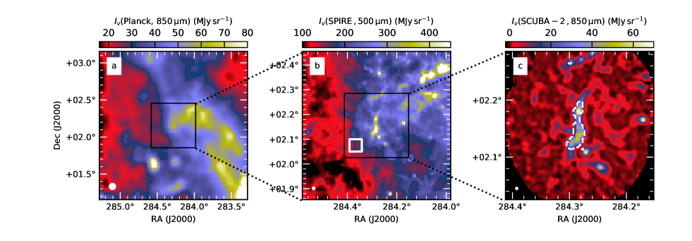
Figure 1: Planck 850 $\mu$m (353 GHz), Herschel 500 $\mu$m, and SCUBA-2/POL-2 850 $\mu$m surface brightness maps of the G035.39-00.33 filament and its surroundings. The beam sizes are indicated in the lower left corner of each frame (5$\arcmin$, 37$\arcsec$, and 14$\arcsec$, respectively). In frame b the white box indicates a reference region for background subtraction. The dashed contour in frame c is drawn at the level of 180 MJy sr^-1 of the background-subtracted 500 $\mu$m surface brightness.

Figure 2 shows surface brightness images from mid-infrared (MIR) to sub-millimetre wavelengths. In addition to Herschel data, the figure shows the 12 $\mu$m surface brightness from the WISE survey (Wright et al. 2010). The filament is seen in absorption up to the 70 $\mu$m band. The 160 $\mu$m image is dominated by warm dust and the main high-column-density structure is not visible, before again appearing in emission at 250 $\mu$m. The ratio of the 100 $\mu$m and 250 $\mu$m dust opacities is $\sim$5, which suggests (although does not directly prove) that the filament is optically thin at 250 $\mu$m. This is later corroborated by the derived $\tau(250\,\mu{\rm m})$ estimates and by independent column density estimates.

The 70 $\mu$m image shows more than ten point-like sources that appear to be associated to the main filament. Only one of them is visible at 12 $\mu$m, showing that they are either in an early stage or otherwise heavily obscured by high column densities. The sources can be identified also in the PACS 160 $\mu$m image but not at 250 $\mu$m, because of the lower resolution and lower sensitivity to high temperatures, many of the sources are blended together or not visible above the extended cold dust emission. The sources were studied by Nguyen Luong et al. (2011), who also estimated their bolometric luminosities. The sources with luminosity (or with an estimated upper limit) above 100 $L_{\sun}$ are marked in Fig. 2b and are listed in Table 5. The numbering refers to that in Nguyen Luong et al. (2011) Table 1. The most luminous source #2 is outside the main filament. The others have bolometric luminosities of the order of $100\,L_{\sun}$. The low dust temperatures indicate that the internal heating caused by these (probably) embedded sources is not very significant.

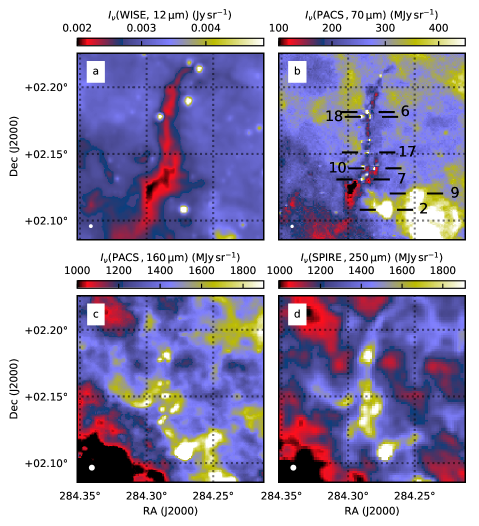
Figure 2: WISE 12 $\mu$m, and Herschel PACS instrument 70 $\mu$m and 160 $\mu$m and SPIRE instrument 250 $\mu$m surface brightness images of G035.39-00.33 . In the 70 $\mu$m image some of the highest-luminosity sources from Nguyen Luong et al. (2011) are indicated.

Table 2: List of the most luminous sources in the G035.39-00.33 field.

#	RA	DEC	$T_{\rm dust}$	$M$	$L$
	(J2000)	(J2000)	(K)	($M_{\sun}$)	(L☉)
2	18:57:05.1	2:06:29	27$\pm$6	24$\pm$16	4700
6	18:57:08.4	2:10:53	16$\pm$3	20$\pm$12	70-200
7	18:57:09.3	2:07:51	12$\pm$1	49$\pm$17	50-130
9	18:56:59.7	2:07:13	22$\pm$4	3 $\pm$1	70-120
17	18:57:08.3	2:09:04	13$\pm$2	50$\pm$19	50-140
18	18:57:07.8	2:10:40	14$\pm$2	20$\pm$9	40-120

2.4 Extinction data

Kainulainen & Tan (2013) calculated for the G035.39-00.33 region high-dynamical-range extinction maps using a combination of NIR observations of reddened background stars and the MIR extinction of extended emission. A NIR extinction map was made at 30$\arcsec$ resolution using UKIDSS data (Lawrence et al. 2007) and an adaptation of the NICER method in Kainulainen et al. (2011) (see also Lombardi & Alves 2001). The assumed extinction curve has $\tau(V)=3.54\,\tau(J)$ (Cardelli et al. 1989). The MIR extinction was measured using Spitzer 8 $\mu$m images from the GLIMPSE survey (Butler & Tan 2012a). This enabled the extension of the estimates to higher column densities and down to a nominal resolution of 2$\arcsec$. The MIR data suffer from spatial filtering (low sensitivity to extended structures) and exhibit some differences relative to the NIR data that could be caused by fluctuations in the brightness of the background (or foreground). Kainulainen & Tan (2013) compensated for these effects by combining the two data sets into a single $A_{\rm V}$ map. The correlation between the NIR and MIR data was best in the $A_{\rm V}=10-15$ mag range while at higher column densities the NIR estimates are, as expected, smaller because the background stars do not provide a good sampling of the highest column densities. The morphology and relative extinction values in the combined extinction map are not dependent on a priori assumptions of the absolute dust opacities but do depend on the assumed opacity ratio of $\kappa(8\,\mu{\rm m})/\kappa({\rm K})=0.29$.

We converted the Kainulainen & Tan (2013) $A_{\rm V}$ estimates (data provided by J. Kainulainen) to J band optical depth $\tau({\rm J})$ using the opacity ratio quoted above. In Sect. 4.3 the $\tau({\rm J})$ map will be compared to observations of dust emission.

3 Methods

3.1 Column density estimates

Basic column density estimates can be derived via modified blackbody (MBB) fits that model the observed intensities as

$$I_{\nu}(\nu)=I_{\nu}(\nu_{0})\frac{B_{\nu}(\nu,T)}{B_{\nu}(\nu_{0},T)}\left(\frac{\nu}{\nu_{0}}\right)^{\beta},$$ (1)

where $B_{\nu}$ is the Planck law, $T$ the colour temperature, $\beta$ the dust opacity spectral index, $I_{\nu}(\nu)$ the observed intensities, and $I_{\nu}(\nu_{0})$ the intensity at the reference frequency $\nu_{0}$. In the MBB fit the free parameters are $I_{\nu}(\nu_{0})$, $T$, and $\beta$, although in many cases the spectral index $\beta$ is kept fixed. With an assumption of the value of $\kappa(\nu_{0})$, the dust opacity relative to the total gas mass, the MBB result can be converted to estimates of the column density,

$$N({\rm H}_{2})=\frac{I_{\nu}(\nu_{0})}{B_{\nu}(T)\kappa(\nu_{0})\,\mu m_{\rm H}}.$$ (2)

Here $\mu$ is the total mass per Hydrogen molecule and $\mu=2.8$ atomic mass units the total gas mass per hydrogen molecule. The mass surface density (g/cm²) is $\Sigma=N({\rm H}_{2})\,\mu$. We adopt dust opacities $\kappa(\nu)=0.1\,(\nu/1000\,GHz)^{\beta}$ cm² g^-1 (Beckwith et al. 1990; Juvela et al. 2012). The above assumes that the observed intensities can be represented by a single MBB formula like in Eq. (1). This is not generally true and, in particular, leads to an underestimation of the column densities of non-isothermal sources (Shetty et al. 2009b; Malinen et al. 2011; Juvela & Ysard 2012b; Juvela et al. 2013a). Equation (1) also explicitly assumes that the emission is optically thin, which is probably the case for G035.39-00.33 observations at wavelengths $\lambda\geq 250$ $\mu$m. For optically thick emission the column density estimates would always be highly unreliable and the use of the full formula instead of the optically thin approximation of Eq. (1) is not likely to improve the accuracy (Malinen et al. 2011; Men’shchikov 2016).

If all the maps used in the fits are first convolved to a common low resolution, the previous formulas provide column density maps at this resolution. We also made column density maps at a higher resolution by making a model that consisted of high-resolution $I_{\nu}(\nu_{0})$ and $T$ maps, keeping the spectral index $\beta$ constant. This model provides predictions at the observed frequencies according to Eq. (1). Each model-predicted map was convolved to the resolution of the corresponding observed map using the convolution kernels described in Sects. 2.1 and 2.2. The minimisation of the weighted least squares residuals provided the final model maps for $I_{\nu}(\nu_{0})$ and $T$. The free parameters thus consisted of the intensity values $I_{\nu}(\nu_{0})$ and the temperature values $T$ of each pixel of the model maps. The chosen pixel size was 6$\arcsec$, more than two times smaller than the resolution of the observed surface brightness maps. Because the solution at a given position depends on the solution at nearby positions, the $I_{\nu}(\nu_{0})$ and $T$ maps need to be estimated through a single optimisation problem rather than for each pixel separately. The optimised model maps were convolved to FWHM_MOD and were then used to calculate column density maps at that same resolution. We used FWHM_MOD=20$\arcsec$, when fitting Herschel data, and FWHM_MOD=15$\arcsec$, when fitting combined Herschel and SCUBA-2 observations. The procedure is discussed further in Appendix A. Because the method is simply fitting the observed surface brightness values, it is still subject to all the caveats regarding the line-of-sight (LOS) temperature variations.

3.2 Polarisation quantities

The polarisation fraction could be calculated as

$$p=\frac{\sqrt{Q^{2}+U^{2}}}{I},$$ (3)

but this estimate is biased because of observational noise and because $p$ depends on the squared sum of $Q$ and $U$. Therefore, we use the modified asymptotic estimator of Plaszczynski et al. (2014),

$$p_{\rm mas}=p-b^{2}\frac{1-\exp(-p^{2}/b^{2})}{2p},$$ (4)

where $b^{2}$ is

$$b^{2}=\frac{\sigma_{U}^{\prime 2}\cos^{2}(2\psi_{0}-\theta)+\sigma_{Q}^{\prime 2}(2\psi_{0}-\theta)}{I_{0}^{2}}\,,$$ (5)

with

$$\theta=\frac{1}{2}\mathrm{atan}\left(\frac{2\sigma_{QU}}{\sigma_{Q}^{2}-\sigma_{U}^{2}}\right)\,,$$ (6)

$$\sigma_{Q}^{\prime 2}=\sigma_{Q}^{2}\cos^{2}\theta+\sigma_{U}^{2}\sin^{2}\theta+\sigma_{QU}\sin 2\theta,$$ (7)

$$\sigma_{U}^{\prime 2}=\sigma_{Q}^{2}\sin^{2}\theta+\sigma_{U}^{2}\cos^{2}\theta-\sigma_{QU}\sin 2\theta.$$ (8)

In Eq. (5) $\psi_{0}$ stands for the true polarisation angle and is in practice replaced by its estimate (see below). The error estimates of $p$ are calculated from

$$\sigma_{p,\rm\,mas}=\sqrt{\sigma_{Q}^{\prime 2}\cos^{2}(2\psi-\theta)+\sigma_{U}^{\prime 2}\sin^{2}(2\psi-\theta)}/I.$$ (9)

(Plaszczynski et al. 2014; Montier et al. 2015b). The $p_{\rm mas}$ estimator is reliable at $p_{\rm mas}/\sigma_{p,\rm mas}>2$ (Montier et al. 2015b). In this paper, polarisation fractions are calculated using the $p_{\rm mas}$ estimator, both in the case of real observations and in the simulations of Appendix C. The only exception is the analysis of radiative transfer models (Sect. 5), because these are free of noise that could affect the $p$ estimates.

The polarisation angle depends on Stokes $Q$ and $U$ as

$$\psi=0.5\arctan(U,Q).$$ (10)

We use the IAU convention where the angle increases from north towards east. The estimated POS magnetic field orientation is obtained by adding $\pi/2$ radians to $\psi$. The uncertainties of $\psi$ are estimated as

$$\sigma_{\psi}=\sqrt{\frac{Q^{2}\sigma_{U}^{2}+U^{2}\sigma_{Q}^{2}-2QU\sigma_{QU}}{Q^{2}\sigma_{Q}^{2}+U^{2}\sigma_{U}^{2}+2QU\sigma_{QU}}}\,\,\frac{\sigma_{p}}{2p}\,{\rm rad},$$ (11)

based on the error estimates of the Stokes parameters $\sigma_{Q}$ and $\sigma_{U}$ and the covariance between Stokes $Q$ and $U$, $\sigma_{QU}$ (Plaszczynski et al. 2014; Montier et al. 2015b). All the quantities in the above formulas are available from the data reduction except for the SCUBA-2 covariances $\sigma_{QU}$, which are set to zero. Montier et al. (2015a) note that the $\psi$ error estimates are reliable for SNR¿4 but can be strongly underestimated for lower SNR because of the bias of the $p$ parameter.

The uniformity of the polarisation vector orientations and thus the regularity of the underlying magnetic field can be characterised with the polarisation angle dispersion function $S$ (Planck Collaboration Int. XIX 2015). It is calculated as a function of position $\bar{r}$ as

$$S(\bar{r},\bar{\delta})=\sqrt{\frac{1}{N}\sum_{i=1}^{N}\left(\psi(\bar{r})-\psi(\bar{r}+\bar{\delta}_{i})\right)^{2}}.$$ (12)

Here $\bar{\delta}_{i}$ is an offset for $N$ map pixels at distances [$\delta/2$, $3\delta/2$] from the central position $\bar{r}$. The scalar $\delta$ thus defines the spatial scale at which the dispersion is estimated. We set the $\delta$ values according to the present data resolution as $\delta=$FWHM/2. The angle difference is calculated directly from the Stokes parameters as

$$\psi(\bar{r})-\psi(\bar{r}+\bar{\delta}_{i})=\arctan(Q_{r}U_{\delta}-Q_{\delta}U_{r},Q_{r}Q_{\delta}+U_{r}U_{\delta})/2,$$ (13)

where the indices $r$ and $\delta$ refer to the positions $\bar{r}$ and $\bar{r}+\bar{\delta}_{i}$, respectively. In the convolution of the Stokes vector images and in the calculation of the polarisation angle dispersion function, we take into account the rotation of the polarisation reference frame as described in Appendix A of Planck Collaboration Int. XIX (2015). However, these corrections are not very significant at the angular scales discussed in this paper. All $S$ values presented in this paper are bias-corrected as $\sqrt{S^{2}-\sigma(S)^{2}}$, where $\sigma(S)$ is the estimated uncertainty for $S$ in Eq.(12) (Planck Collaboration Int. XIX 2015).

3.3 Radiative transfer models

We complemented the analysis described in Sects. 3.1 and 3.2 with radiative transfer (RT) calculations. These have the advantage of providing a more realistic description of the temperature variations and, in the case of polarisation, allow the explicit testing of the effects of imperfect grain alignment and different magnetic field geometries.

The models cover an area of $13\arcmin\times 13\arcmin$ on the sky with a regular grid where the size of the volume elements corresponds to 6$\arcsec$. The LOS density profile was assumed to have a functional form of $n(z)\propto(1+(z/R)^{2})^{p/2}$, where $z$ is the LOS coordinate. With parameters $R=0.16$ pc and $p=2$ this gives for the filament similar extent in the LOS direction as observed in the POS. Such a short LOS extent is appropriate only for the densest regions. Therefore, we used a scaled LOS coordinate $z/z_{N}$ where $z_{N}$ is linear with respect to the logarithm of the column density and increases from 1 for $N>5\times 10^{22}$ cm^-2 to 5 for a factor of ten smaller column densities.

The RT model initially corresponded to the column densities estimated from MBB fits at 40$\arcsec$ resolution. The cloud was illuminated by the normal interstellar radiation field (ISRF) according to the Mathis et al. (1983) model. The dust properties were taken from Compiègne et al. (2011) but the dust opacity at wavelengths $\lambda>100\mu$m were increased to give $\tau(250\,\mu{\rm m})/\tau({\rm J})$ ratios of $10^{-3}$ or $1.6\times 10^{-3}$. The extinction curve was rescaled to give the same $\kappa(250\,\mu{\rm m})$ value as quoted in Sect. 3.1. The latter scaling has no real effect on the RT modelling itself but simplifies the comparison with values derived from observations.

The models were optimised to match a set of surface brightness observations. The free parameters included the scaling of the column densities, one parameter per a 6$\arcsec$ map pixel, and the scaling of the external radiation field, $k_{ISRF}$. The G035.39-00.33 region includes a number of radiation sources with luminosities $\sim 10\,{\rm L}_{\sun}$ or less. Because their location along the line of sight is not known, the qualitative effects of internal heating were tested by including in the model an optional diffuse emission component. The diffuse emission has the same spectrum as the external radiation field and it was scaled with a parameter $k_{\rm diff}$, the value of 1 corresponding to a bolometric luminosity of 1 $L_{\sun}\,{\rm pc}^{-3}$.

The radiative transfer problem was solved with the Monte Carlo program SOC (Juvela et al. in prep.; Gordon et al. 2017). Because the fitted observations are at long wavelengths $\lambda\geq 250\,\mu$m, the dust grains were assumed to be in equilibrium with the radiation field and the emission from stochastically heated grains was omitted. SOC calculates the dust temperatures based on the radiative transfer simulation and writes out surface brightness maps at the requested wavelengths.

SOC can be used to calculate estimates of the polarised dust emission. This was done using grain alignment that was either constant, had an ad hoc density-dependence, or was predicted by RAT calculations (Lazarian & Hoang 2007). For the RAT case, the radiative transfer modelling provided the intensity and anisotropy of the radiation field, which were then used to estimate the minimum size of aligned grains and thus a reduction factor $R$ for the polarised emission originating in each model cell. The calculations were done as described in Pelkonen et al. (2009). The polarisation signal is dependent on the minimum size of the grains that remain aligned in a magnetic field. This is dependent on the ratio between the angular velocity produced by the radiation field and the thermal rotation rate,

$$\left(\frac{\omega_{\rm rad}}{\omega_{\rm T}}\right)^{2}\propto\frac{a}{(n_{\rm H}T)^{2}}\left[\int(Q_{\Gamma}\cdot\hat{a})\lambda J_{\lambda}d\lambda\right]^{2},$$ (14)

where $n_{\rm H}$ is the volume density, $T$ the temperature, $a$ the grain size, $Q_{\Gamma}$ the wavelength-dependent efficiency of RAT (dependent on the grain properties), $\hat{a}$ the unit vector of the rotational axis, and $J_{\lambda}$ the radiation field intensity. Thus, grain alignment is promoted by larger grain sizes and larger intensity and anisotropy of the radiation field. Conversely, higher density and temperature tend to reduce the grain alignment and subsequently the polarised intensity.

Given a model of the 3D magnetic field within the model volume, SOC gives synthetic maps for $I$, $Q$, and $U$. We used these to examine the effect that imperfect grain alignment can have on the observed polarisation fraction distributions. For comparison with the full calculations with grain alignment, synthetic maps were also produced assuming a constant value of $R$ or an ad hoc density dependence of $R$.

4 Results

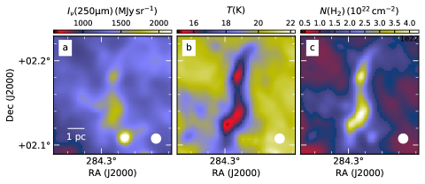
Figure 3: Results of modified blackbody fits to SPIRE data at 40$\arcsec$ resolution and without background subtraction: 250 $\mu$m intensity (frame a), colour temperature (frame b), and column density (frame c).

4.1 Herschel data

Figure 3 shows the results of MBB fits using SPIRE surface brightness maps at 40$\arcsec$ resolution. The fits were done to data before background subtraction and thus correspond to emission from the full LOS. The extended cloud component has a significant contribution of almost $N({\rm H}_{2})=10^{22}$ cm^-2 to the total column density. The peak column densities of both the northern and the southern parts are $N({\rm H}_{2})\sim 4\times 10^{22}$ cm^-2. The colour temperatures are 20-21 K in the background, below 18 K within the dense filament ($N({\rm H}_{2})>2\times 10^{22}$ cm^-2), and reach minimum values of 15.5 K and 15.2 K in the northern and southern clumps, respectively. PACS data were not used (see Sect. 2.2), but at the temperatures of the main filament ($T\sim$15 K), the Herschel 250 $\mu$m, 350 $\mu$m, and 500 $\mu$m SPIRE bands give reliable measurements of the dust colour temperature (see Juvela et al. 2012). On the other hand, they do not give strong simultaneous constraints for both the colour temperature and the spectral index. Therefore, the SPIRE data were fitted using a constant value of $\beta$=1.8.

We created column density maps at a resolution of 20$\arcsec$, as described in Sect. 3.1 using background-subtracted data. The background was determined as the average signal in a $3\arcmin\times 3\arcmin$ area centred at RA=18^h57^m28^s, DEC=2$\degr 4\arcmin 30\arcsec$ (see Fig. 1b). Compared to Fig. 3, the filament is colder, mainly because of the background subtraction (see Fig. 4). The minimum temperatures are 12.4 K in the northern and 11.7 K in the southern part (13.7 K and 12.7 K, respectively, if this map is convolved down to 40$\arcsec$ resolution). At the 20$\arcsec$ resolution the fitted $I_{\nu}(250\,\mu{\rm m})$ map shows local maxima at the positions of the MIR sources (Fig. 2b) but are not similarly visible in column density. In spite of the background subtraction, the peak column densities are higher, slightly above $5\times 10^{22}$ cm^-2 in both the northern and the southern parts. This is a consequence of the lower colour temperatures. The column densities are probably still underestimated because of LOS temperature variations. We will refer to this version of the column density map as $N_{3}({\rm H}_{2})$, the sub-index referring to the number of bands fitted.

Unlike in the standard MBB fits that are done for each pixel separately, Fig. 4 corresponds to a global fit over the map. The fit residuals (Fig. 4d-f) are dominated by small-scale artefacts (below the beam size) that are connected with the finite pixel size and possibly with imperfections in the beam model. If these residual maps are convolved to the resolution of the observations, they are smooth with peak-to-peak errors below $\sim$4%.

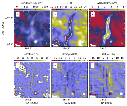
Figure 4: Results of modified blackbody fits to SPIRE data at a resolution of 20$\arcsec$. The upper frames show the fitted 250 $\mu$m intensity, dust colour temperature, and column density. The lower frames show the relative error of the fits for the individual SPIRE bands. We have masked a region in the SE corner where the background-subtracted 250 $\mu$m intensities are below 10 MJy sr^-1. The beam sizes of the observations are shown in the bottom right-hand corner of each frame. The contours are drawn at $T$=13.5 K and $N({\rm H}_{2})=2\times 10^{22}\,{\rm cm}^{-2}$.

4.2 Combined Herschel and SCUBA-2 data

We estimated the average SED of the main filament using band-to-band correlations. We selected data where the background-subtracted SPIRE 500 $\mu$m values were above of 180 MJy sr^-1 (see Fig. 1c), further dividing the filament into a northern and a southern part along $\delta=2\degr 10\arcmin$. The data were convolved to the resolution of the 500 $\mu$m band, each band was correlated with the 350 $\mu$m data, and the uncertainties of the linear fits were estimated with bootstrapping. The correlations in the northern and the southern regions and the SED fit to the combined data are shown in Fig. 5.

The data were fitted with MBB functions using the Markov chain Monte Carlo method and flat priors with temperatures in the range 7-30 K and spectral indices in the range 0.5-3.5. Fits to all five bands gave $T=11.29\pm 0.83$ K, $\beta=2.06\pm 0.22$ for the southern part, $T=12.46\pm 0.95$ K, $\beta=1.82\pm 0.24$ for the northern part, and $T=11.92\pm 0.87$ K, $\beta=1.94\pm 0.22$ for the combined data. In this last case, the fitted SED consisted of the weighted average of the SEDs points of the southern and northern parts. The effects from the spatial filtering of the SCUBA-2 data should be small because the selected data only cover a $\sim 1.5\arcmin$ wide part of the filament. The 450 $\mu$m SCUBA-2 point of the northern region is significantly above the fitted SED. However, if this point is omitted, the spectral index estimate remains almost unchanged, $\beta=1.95$. The fit to the three SPIRE channels without SCUBA-2 data gave $T=12.66\pm 1.42$ K, $\beta=1.76\pm 0.33$.

We fitted the SPIRE and the 850 $\mu$m data also with a model that had one free parameter for $\beta$, one free parameter for the relative offset of the 850 $\mu$m surface brightness map, and one free parameter for the colour temperature in each pixel. We used the same relative uncertainties as above but further assumed a correlation $\rho=0.5$ between the errors of the SPIRE channels. Unlike in the previous surface brightness correlations, the fit relies on the consistency of the intensity zero points of the background-subtracted SPIRE maps. The results from Markov chain Monte Carlo calculations were $\beta=1.84\pm 0.02$ for the southern part and $\beta=1.69\pm 0.02$ for the northern part. These are close to the SPIRE-only fits, partly because the SCUBA-2 data have less leverage on the $\beta$ values once the 850 $\mu$m surface brightness offset is included as a separate free parameter. All error estimates above correspond to the 4% (SPIRE) and 10% (SCUBA-2) uncertainties of the surface brightness measurements. The true uncertainties can be larger because of the systematic errors.

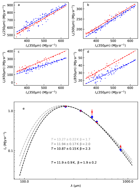
Figure 5: SEDs from the correlations of surface brightness values over the main filament. Frames a-d show the band-to-band correlations for the northern (red) and southern (blue) parts of the filaments. The points correspond to an oversampling by a factor of two relative to the data resolution. Frame e shows the resulting SEDs and modified blackbody fits to the combined data for three fixed values of the spectral index $\beta$. The result for a fit with free $\beta$ are shown below the results of the fixed-$\beta$ fits.

We fitted the three SPIRE and two SCUBA-2 bands together to derive maps of dust colour temperature and of optical depth at 15$\arcsec$ resolution, under the assumption of $\beta=1.8$. The optimisation procedure is the same as in Sect. 4.1 (see Sect. refmethods:MBB). We used background-subtracted SPIRE data but also had to correct the zero points of the SCUBA-2 data. This was done by taking the predictions of SPIRE fits with $\beta=1.8$ at the wavelengths 450 $\mu$m and 850 $\mu$m and comparing these to the SCUBA-2 maps at the same resolution. The 450 $\mu$m offset was calculated using the average surface brightness values of the pixels where the original SCUBA-2 450 $\mu$m value was above 160 MJy sr^-1. For the 850 $\mu$m map the corresponding threshold was 30 MJy sr^-1. These offset-corrected maps were used as additional constraints in the area where the signal was above the quoted surface brightness thresholds. This means that SCUBA-2 data were used over a narrow region around the main filament where the loss of low spatial frequencies should be small. Because the offsets were based on the SPIRE SEDs, these data cannot be used to draw any conclusions on the SED shape at wavelengths beyond 500 $\mu$m. The SCUBA-2 data only provide additional constraints on the small-scale column density structure. The resulting 250 $\mu$m optical depth estimates are referred to as $\tau_{5}(250\,\mu{\rm m})$ and the column density estimates as $N_{5}({\rm H}_{2})$.

The results are shown in Fig. 6 at the resolution of FWHM=15$\arcsec$ (Gaussian beam). In principle, this is the resolution also outside the main filament, where SCUBA-2 data were not used. However, there FWHM=15 $\arcsec$ corresponds to a deconvolution below the SPIRE resolution and the small-scale structure is not reliable. The peak column densities are $7.2\times 10^{22}$ cm^-2 and $7.0\times 10^{22}$ cm^-2 for the northern and the southern part, respectively. Unlike in Fig. 4, there are several local column density maxima NW of the southern clump that are related to the 70–250 $\mu$m sources of Fig. 2. They are more visible because of the higher resolution (15$\arcsec$ vs. 20$\arcsec$). However, if the effective resolution of the fitted temperature map (which is dependent on longer-wavelength SPIRE channels) is lower than the effective resolution of the fitted surface brightness map, the column density estimates could be biased upwards at the location of warm point-like sources.

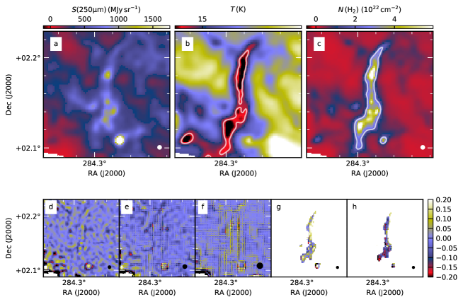
Figure 6: Modified blackbody fit to the combined SPIRE and SCUBA-2 data at 15$\arcsec$ resolution, using SCUBA-2 data as a constraint only over the main filament. Frames a-c show the fitted 250 $\mu$m surface brightness, the colour temperature, and the estimated column density. The frames d-h show the residuals relative to the observed, background-subtracted surface brightness values at 250, 350, 500, 450, and 850 $\mu$m, respectively. The fits used $\beta=1.8$. The contours are drawn at $T$=13.5 K and $N({\rm H}_{2})=2\times 10^{22}\,{\rm cm}^{-2}$.

4.3 Dust opacity

The extinction map of Kainulainen & Tan (2013) (Sect. 2.4) enables us to compare dust opacities between the NIR/MIR and sub-millimetre regimes. The correlations of these $\tau({\rm J})$ values with the $\tau_{5}(250\,\mu{\rm m})$ optical depth estimates are shown in Fig. 7.

The least squares fit gave an average ratio of $\tau(250\,\mu{\rm m})/\tau({\rm J})=(2.55\pm 0.03)\times 10^{-3}$. The error estimate only refers to the uncertainty of the fit itself, which was estimated by bootstrapping. The relation is found to be steeper in the northern clump and shallower $\tau({\rm J})<6$ (see Fig. 7).

In addition to the correlation plot of Fig. 7, we estimated the $\tau(250\,\mu{\rm m})/\tau({\rm J})$ ratio based on the absolute values. We subtracted from the $\tau({\rm J})$ and $\tau(250\,\mu{\rm m})$ maps a background that was estimated as the average along a 1$\arcmin$-wide boundary that follows the contour in Fig. 7a. After the subtraction of the local background, the average values inside the contour gave $\tau(250\,\mu{\rm m}))/\tau({\rm J})=(2.1\pm 0.5)\times 10^{-3}$. The error estimate is based on the total signal fluctuations over the area used for background subtraction.

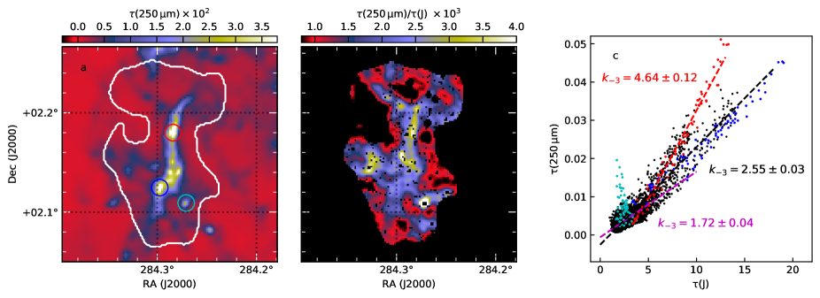
Figure 7: Comparison of $\tau(250\mu{\rm m})$ and $\tau({\rm J})$ estimates: the $\tau(250\mu{\rm m})$ map (frame a), the ratio $k_{-3}=10^{-3}\times\tau(250\mu{\rm m})/\tau({\rm J})$ (frame b), and the same ratio as a correlation plot (frame c). The last two frames are limited to data in the area indicated in the first frame, also excluding pixels for which $\tau({\rm J})$ is not defined because of masked stars. Selected $30\arcsec$ radius regions (see frame a) are marked in frame c with different colours: a point source SE of the southern clump (cyan) and the northern and southern $\tau(250\mu{\rm m})$ peaks (red and blue circles, respectively). The black line in frame c is a least squares fit to the data, only excluding the SE point source. Fits to the northern clump and to data $\tau({\rm J})<6$ are shown in red and magenta, respectively.

4.4 Polarisation data

Figure 8 shows an overview of the Planck and POL-2 polarisation data. Planck maps have very little noise. When POL-2 data are convolved to a 40$\arcsec$ resolution, the polarisation angle dispersion $S$ is clearly affected by noise outside the $N({\rm H}_{2})=10^{22}\,{\rm cm}^{-2}$ contour and $p$ becomes dominated by noise closer to the map edges. At the higher 20$\arcsec$ resolution, polarisation fraction values become uncertain as soon as column density drops below $N({\rm H}_{2})=10^{22}\,{\rm cm}^{-2}$.

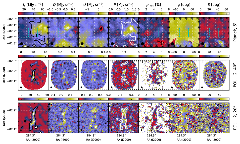
Figure 8: Overview of polarisation data of the G035.39-00.33 region. The three rows show, respectively, Planck data at 5$\arcmin$ resolution, POL-2 data at 40$\arcsec$ resolution, and POL-2 data at 20$\arcsec$ resolution. The seven frames on each row are: $I$, $Q$, $U$, polarised intensity $P$, polarisation fraction $p_{\rm mas}$, polarisation angle $\psi$, and polarisation angle dispersion function $S$ for a lag of $\delta=$FWHM/2. The dashed boxes on Planck maps correspond to the size of the second row images. The column densities $N({\rm H}_{2})=10^{22}\,{\rm cm}^{-2}$ (at the corresponding resolutions) are indicated with contours on the $I$ maps. On the second and third row these are calculated from background-subtracted Herschel and SCUBA-2 data. The white contours on the $P$ maps correspond to an intensity $I(850\,\mu{\rm m})$ of 40 MJy sr^-1 on the Planck map and 10 MJy sr^-1 on the POL-2 maps.

Figure 9 shows histograms for the SNR of polarisation fraction, $p_{\rm mas}/\sigma_{p,\rm mas}$. The plot includes histograms for Planck data at 5$\arcmin$ resolution and for the POL-2 data at 20$\arcsec$ and 40$\arcsec$ resolutions. According to Montier et al. (2015b), $p_{\rm mas}$ is unbiased for $p_{\rm mas}/\sigma_{p,\rm mas}>2$. The SNR is sufficient for almost all Planck data at the full resolution and most of the POL-2 data at 40$\arcsec$ resolution, when selected at $N({\rm H_{2}})>10^{22}$ cm^-2. Data cannot be thresholded directly using the SNR because that would lead to a biased selection of $p$ values (Planck Collaboration XII 2018). Figure 9c shows that at 20$\arcsec$ resolution a significant part of POL-2 $p_{\rm mas}$ estimates may be biased (at SNR$<$2 the modified asymptotic estimator may not remove all the bias in $p$) and a higher column density threshold does not fully remove the problem.

The polarisation angle estimates are mainly unbiased but since they are affected by noise, at low SNR the polarisation angle dispersion function $S$ will have systematic positive errors that are not fully removed by the bias correction. The appearance of the Fig. 8 maps is in qualitative agreement with this.

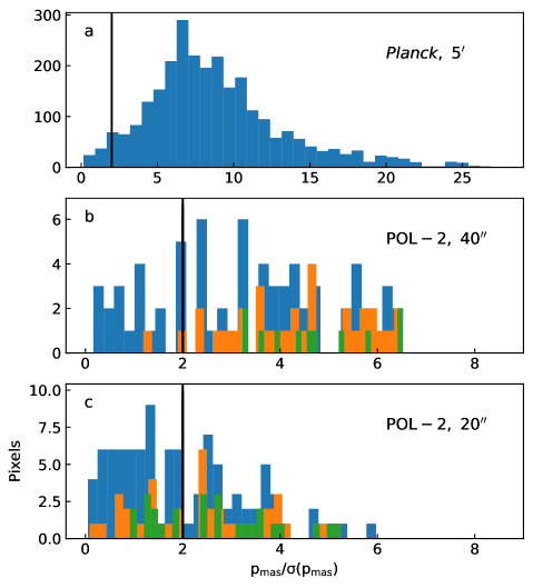
Figure 9: SNR of polarisation fraction. The frames correspond to Planck data at 5$\arcmin$ resolution (frame a) and to POL-2 data at 40$\arcsec$ (frame b) and 20$\arcsec$ (frame c) resolution. Frame a includes all data over a $2\degr\times 2\degr$ area. In frames b-c, histograms show POL-2 data above column density thresholds of 1, 2, and 3 times $N({\rm H_{2}})=10^{22}$ cm^-2 (blue, orange, and green histograms, respectively). Vertical lines at 2 indicate an approximate limit above which the $p_{\rm mas}$ estimates are reliable. All data are sampled at steps FWHM/2.

4.5 Magnetic field geometry

The magnetic field geometry of the cloud G035.39-00.33 has been discussed in detail in Liu et al. (2018b) based on the POL-2 observations. However, we present some plots on the magnetic field morphology before concentrating on the polarisation fraction in the following sections.

Figure 10a shows a large-scale polarisation map based on Planck 850 $\mu$m. This is dominated by a regular field that in equatorial coordinates runs from NE to SW. At the 5$\arcmin$ resolution the G035.39-00.33 filament is not prominent because of the strong background emission (see Fig. 1). The SCUBA-2 850 $\mu$m surface brightness map in Fig. 11a shows the main ridge and some other filamentary features that were discussed in Liu et al. (2018b). At this $\sim 14\arcsec$ resolution the polarisation vectors show a less ordered field. In the central part, the field is partly perpendicular to the filament. In the north, the field turns parallel to the filament and is thus almost perpendicular to the large-scale field observed by Planck. The SE-NW orientation observed in the northern end is actually common to filament boundary regions and is particularly clear on the eastern side.

The second frames in Figs. 10-11 show maps of the bias-corrected polarisation angle dispersion function $S$. For Planck these are calculated at the scale of $\delta=2.5\arcmin$ using the Planck observations at their native resolution of FWHM=5$\arcmin$. In the case of SCUBA-2, to increase the SNR, the data were smoothed to a resolution of 40$\arcsec$ and $S$ was calculated with $\delta=20\arcsec$. Figure 11 shows that in POL-2 observations $S(20\arcsec)$ goes in some areas below $\sim$10$\degr$. Higher values are found for example in the northern clump. There the change in the magnetic field orientation coincides with the intensity maximum and large $S$ avalues are not produced by noise alone. Similarly, at the eastern filament edge, the polarisation angles are uniform along the boundary but change systematically between the high and low column densities, contributing to the variation seen inside the $N({\rm H}_{2})=10^{22}$ cm^-2 contour.

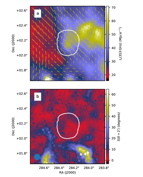
Figure 10: Planck 850 $\mu$m (353 GHz) surface brightness with vectors showing the POS magnetic field orientation (frame a) and polarisation angle dispersion function $S(\delta=2.5\arcmin)$ calculated from Planck data (frame b). The maps are at the original $5\arcmin$ resolution. The white contours indicate the area covered by SCUBA-2 observations. The length of the polarisation vectors is proportional to the polarisation fraction (90$\arcsec$ for 1% of polarisation).

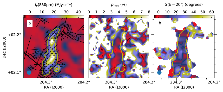
Figure 11: Field orientation on the POL-2 850 $\mu$m intensity map (frame a), polarisation fraction $p_{\rm mas}$ (frame b), and polarisation angle dispersion function $S(\delta=20\arcsec)$ (frame c) calculated from data at 40$\arcsec$ resolution. Polarisation vectors (at 20$\arcsec$ steps, rotated to show the magnetic field orientation) and $S$ are shown for pixels with $N({\rm H_{2}})>5\times 10^{21}$ cm^-2. The length of the polarisation vectors per cm is the same as in Fig. 10 (14.4$\arcsec$ for a polarisation fraction of 1%). The yellow contours correspond to $N({\rm H_{2}})=10^{22}$ cm^-2, outside of which polarisation angles are uncertain.

The Planck polarisation vectors are quite uniform over the G035.39-00.33 filament while the field geometry in SCUBA-2 850 $\mu$m data is different and partly orthogonal. One may ask whether the observations are consistent or whether the locally changing magnetic field orientation should be visible in Planck data as a drop in the polarisation fraction. We tested this by making simultaneous fits to the $I$, $Q$, and $U$ data of both Planck and SCUBA-2. The results in Appendix B show that the observations are not contradictory. This is possible because of the large difference in the beam sizes and because the SCUBA-2 data are not sensitive to emission at scales larger than 200$\arcsec$. Thus, most information about the large-scale field is filtered out in the SCUBA-2 data.

4.6 Polarisation fraction

4.6.1 Polarisation fraction from Planck observations

Figure 12 shows the bias-corrected polarisation fraction estimate $p_{\rm mas}$ from Planck observations over a $1\degr\times 1\degr$ region and at a resolution of 5$\arcmin$. The average value is $p\sim$2%. For comparison, the Herschel column density map was convolved to the same resolution but the polarisation fraction does not show clear dependence on the column density. At this resolution, the G035.39-00.33 filament shows up in the column density map only as a minor local maximum and the polarised signal appears to be dominated by more extended emission components. The polarisation fraction values at the filament location are slightly higher than in the region on average, close to $2.5\%$ as indicated in Fig. 12d.

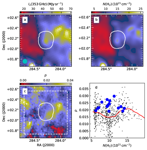
Figure 12: Polarisation fraction of the G035.39-00.33 region based on Planck data. Frame a shows the 850 $\mu$m surface brightness, frame b the Herschel column density map convolved to 5$\arcmin$ resolution, and frame c a map of the polarisation fraction $p_{\rm mas}$ from Planck data. The white contour indicates the coverage of the SCUBA-2 map. Frame d shows the polarisation fraction as a function of column density, sampled with 2$\arcmin$ steps from maps at 5$\arcmin$ resolution, excluding the map boundaries (indicated by dashed lines in Frame c), without a SNR cut-off. The red line is the running mean and the blue circles show values from the area covered by SCUBA-2 observations.

We examine in Fig. 13 how, in the case of Planck data, the bias-corrected polarisation fraction and the estimated polarisation angle dispersion function depend on the column density and on the data resolution. The changes from $5\arcmin$ to $9\arcmin$ and further to $15\arcmin$ resolution each correspond to about a factor of three increase of SNR. Irrespective of the resolution (and SNR), the mode of $S$ is close to 10% and the values in area covered by SCUBA-2 are of similar magnitude. The polarisation fraction is mainly between 0.5% and 3% and there is no significant difference between the 9$\arcmin$ and 15$\arcmin$ resolution cases. The $p$ values within the area mapped with SCUBA-2 are higher than on average, 2-2.5% for the full-resolution data and $\sim 2$% at lower resolutions. In the same region $S$ tends to be lower than average. This anticorrelation between $p$ and $S$ is clear in Fig. 13c. This could have its origin in either the noise (which increases the estimates of both quantities) or in the magnetic field geometry. The effects of noise has been characterised in previous Planck studies (Planck Collaboration Int. XIX 2015), and should here be small when data are smoothed to increase the SNR. The relation are similar for FWHM=$9\arcmin$ and FWHM=$15\arcmin$, which shows that the results are not severely affected by noise. This is confirmed with simulations in in Appendix C. For given $p$, the $S$ values are lower than previously found with BLASTPol for the Vela C molecular (Fissel et al. 2016) and with Planck for the Gould Belt clouds (Planck Collaboration XII 2018).

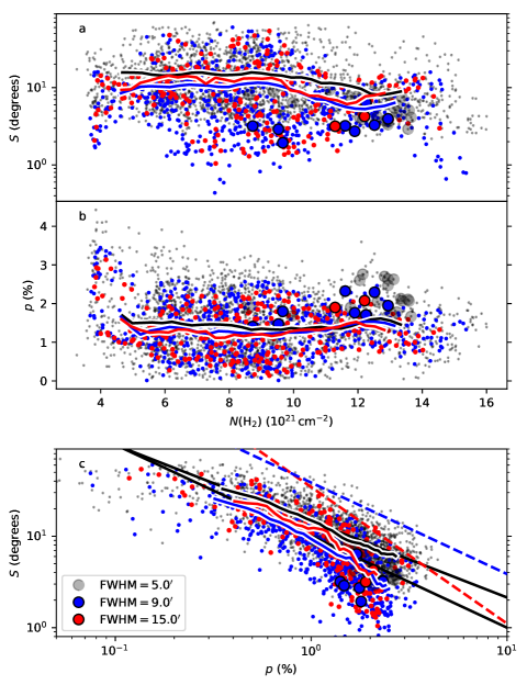
Figure 13: Polarisation angle dispersion function $S$ and polarisation fraction $p_{\rm mas}$ from Planck data in a $2\degr\times 2\degr$ area centred on the POL-2 field. Frames a and b show these as a function of dust optical depth and frame c shows their mutual correlation. The colours of the plot symbols correspond to the data resolution, as indicated in frame c. The solid lines show the corresponding moving averages. The points inside the area mapped with POL-2 are plotted with large symbols. The data are sampled at steps of FWHM/2 and $S$ is calculated for lag $\delta=$FWHM/2. In frame c the upper solid black line shows the relation $\log_{10}(S)=-0.834\times\log_{10}(p_{\rm mas})-0.504$ from Planck Collaboration Int. XIX (2015) and the lower black line the relation $S=0.1/p_{\rm mas}$. The red dashed line is the relation $\log\,p_{\rm mas}=-0.670\log\,S-0.97$ from Fissel et al. (2016). The blue dashed line corresponds to the fit to Gould Belt cloud data, $S\times p=0.31^{\degr}({\rm FWHM}/160\arcmin)^{0.18}$ of Planck Collaboration XII (2018), calculated with FWHM=9$\arcmin$.

4.6.2 Polarisation fraction in SCUBA-2 observations

We calculated the bias-corrected polarisation fraction estimates $p_{\rm mas}$ from SCUBA-2 ($I$, $Q$, $U$) maps that were first convolved to a resolution of $40\arcsec$ to increase their SNR. In Fig. 14 we plot $p_{\rm mas}$ as a function of column density for with $N({\rm H}_{2})>10^{22}$ cm^-2. We avoid a criterion based on the SNR of the polarised intensity because that would bias the selection of the polarisation fraction values. Based on Fig. 9, the plotted $p_{\rm mas}$ values should be unbiased. The average $p_{\rm mas}$ value decreases as a function of $N$ and, based on the formal uncertainty of the weighted least squares fit, the decrease is significant.

The pixels associated to 70 $\mu$m sources (Fig. 14a) do not differ from the general distribution. However, at lower column densities (not shown), they tend to trace the lower envelope of the ($N$, $p_{\rm mas}$) distribution. This is mostly a result of them having on average $\sim$80% higher SNR (higher intensity for a given column density). This makes their $p$ estimates less biased.

Appendix C shows further how the $p_{\rm mas}$ vs. $N$ relation changes as a function of resolution and, consequently, as a function of the SNR. There we also present simulations of the $p_{\rm mas}$ vs. $N$ relation in the presence of noise. These show that while the noise produces significant scatter, the average $p_{\rm mas}$ values estimated at the highest column densities are reliable.

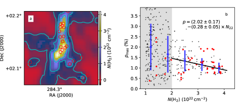
Figure 14: POL-2 polarisation fraction and column density. Frame a shows the column density map $N_{5}({\rm H}_{2})$ at 40$\arcsec$ resolution. The contours are drawn at 0.5, 1, and 2 times $10^{22}$ cm^-2 and the red circles denote the locations of the point sources of Table 5. In frame b, $p_{\rm mas}$ is plotted as a function of column density for data with $N({\rm H}_{2})>10^{22}$ cm^-2. The pixels coinciding with point sources (red circles of Frame a) are plotted in red. The blue bars are representative error estimates. The result of the weighted least squares fit to data at $N({\rm H}_{2})>2\times 10^{22}$ cm^-2 is given in the frame and is shown as a black solid line. The shading corresponds to $N({\rm H}_{2})<2\times 10^{22}$ cm^-2 where the $p_{\rm mas}$ estimates may be biased.

The correlations between $p_{\rm mas}$, $S$, and $N({\rm H}_{2})$ and their dependence on the data resolution are further examined in Fig. 15. The values are independent of the resolution only towards the highest column densities. Otherwise $p_{\rm mas}$ and $S$ decrease with lower resolution. This is consistent with the increasing SNR reducing the bias and data below $N({\rm H}_{2})\sim 10^{22}\,{\rm cm}^{-2}$ remaining affected by noise. However, there may be additional effects from the averaging of observations with different polarisation angles (geometrical depolarisation). The $S$ values may reflect the fact that the G035.39-00.33 field consists of a single, very narrow filament. For a given column density, a larger lag means that $S$ calculation uses data over a larger area and thus on average with a lower SNR.

Figure 15d shows the correlation of $S$ vs. $p_{\rm mas}$. For column densities $N({\rm H}_{2})>2\times 10^{22}\,{\rm cm}^{-2}$, with lower resolution (higher SNR) the values converge towards similar parameter combinations as in Fig. 13 for Planck . This in spite of the fact that the Planck result is for a much larger area and for a data resolution lower by almost a factor of 4. Because of the small dynamical range (in part due to the spatial filtering) and possible residual bias in $S$, no clear anticorrelation is seen between the POL-2 estimates of $p$ and $S$.

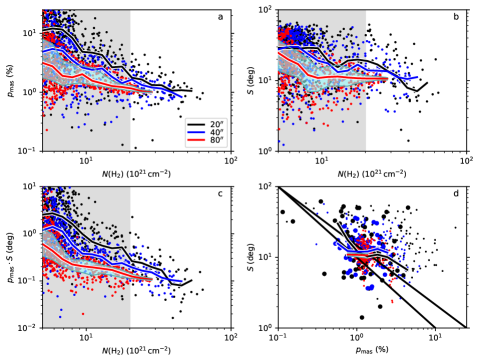
Figure 15: Correlations between POL-2 polarisation parameters $p_{\rm mas}$ and $S$ and the column density. The quantities are calculated at four spatial resolutions represented with the colours indicated in frame a. The data are sampled at steps of FWHM/2 and the solid lines correspond to running averages. In frames a-d, the shading corresponds to $N({\rm H}_{2})<2\times 10^{22}\,{\rm cm}^{-2}$ where, according to Fig. 9, the 40$\arcsec$ resolution $p_{\rm mas}$ estimates become unreliable. In frame d, values for $10^{22}\,{\rm cm}^{-2}<N({\rm H}_{2})<2\times 10^{22}\,{\rm cm}^{-2}$, and $N({\rm H}_{2})>2\times 10^{22}\,{\rm cm}^{-2}$, are shown with small and large symbols, respectively, and the lines show running averages for the higher column density interval (20 logarithmic bins over the parameter range with a minimum of 4 points per bin). Shaded cyan region corresponds to the interquartile range of the quantities plotted with red lines. In frame d the upper solid black line shows the relation $\log_{10}(S)=-0.834\times\log_{10}(p_{\rm mas})-0.504$ from Planck Collaboration Int. XIX (2015) and the lower black line the relation $S=0.1/p_{\rm mas}$.

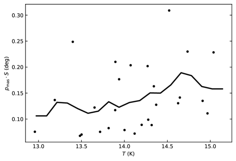
Figure 16: Product $p\times S$ as a function of dust colour temperature. The data are at 40$\arcsec$ resolution, sampled at half-beam steps, and selected from the region with $N({\rm H}_{2})>2\times 10^{22}\,{\rm cm}^{-2}$. The solid lines shows a moving average.

If the $p$-$N$ anticorrelation were due to a loss of grain alignment, the product $p\times S$ should decrease as a function of increasing column density and decreasing dust temperature. Figure 15c shows the anticorrelation with the column density. In Fig. 16 we show the corresponding correlation of $p\times S$ with the dust colour temperature. Although the data selection (resolution of 40$\arcsec$ and column densities $N({\rm H}_{2})>2\times 10^{22}\,{\rm cm}^{-2}$) should ensure that $p$ values are unbiased, the polarisation angle dispersion function $S$ may still contain some bias that contributes to increased $p\times S$ values at higher temperatures, which mainly correspond to lower column densities. The dispersion is calculated using data from an area with a diameter of $1.5\times$FWHM. Therefore, high $N$ at the central position does not fully preclude the $S$ estimate being affected by lower SNR pixels further out. A Monte Carlo simulation based on the $I$, $Q$, and $U$ maps and their error maps shows that the trend in Fig. 16 is not significant and thus neither proves or disproves the presence of grain alignment variations.

5 Radiative transfer models

5.1 Radiative transfer modelling of total emission

Figure 17 compares the column densities of two RT models fitted to SPIRE data. These differ regarding the assumed sub-millimetre vs. NIR opacity but have identical opacity at 250 $\mu$m. The model $A$ has an opacity ratio of $\tau(250\,\mu{\rm m})/\tau({\rm J})=1.6\times 10^{-3}$. This value is the average value derived for a sample of PGCC clumps in Juvela et al. (2015b) and a lower limit for the values estimated in Sect. 4.3. To test the sensitivity to dust properties, the alternative model $B$ has $\tau(250\,\mu{\rm m})/\tau({\rm J})=1.0\times 10^{-3}$. Model $B$ results in 20% higher $\chi^{2}$ values but both models represent the surface brightness data of the main filament equally well. The lower $\tau(250\,\mu{\rm m})/\tau({\rm J})$ ratio leads to higher column densities, with a 30% difference in the densest regions. The effect is thus of similar magnitude as the change in the assumed opacity ratio.

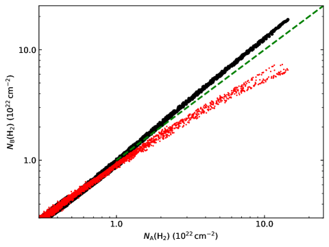
Figure 17: Correlation between the column densities $N({\rm H}_{2})$ of two RT models fitted to observations. Column densities $N_{\rm A}$ and $N_{\rm B}$ (black dots) correspond to dust models with $\tau(250\,\mu{\rm m})/\tau({\rm J})$ equal to $1.6\times 10^{-3}$ and $1.0\times 10^{-3}$, respectively. For the RT model with column densities $N_{\rm A}$, the red points show the column density estimates derived from the synthetic surface brightness maps. The dashed line is the one-to-one relation. All data are at $20\arcsec$ resolution.

Figure 17 also shows $N({\rm H}_{2})$ estimates that were calculated using MBB fits and the simulated surface brightness maps of the model A. As expected, the values recovered with MBB calculations are below the true values. The difference becomes noticeable above $N({\rm H}_{2})=2\times 10^{22}$ cm^-2 and at $N({\rm H}_{2})=10^{23}$ cm^-2 the error is a factor of two.

5.2 Radiative transfer modelling of the $p$ vs. $N$ relation

We added to model $A$ (see Sect. 5.1) alternative descriptions of the magnetic field geometry to make predictions of the polarised emission. These calculations are used to test how the field geometry could affect the observed polarisation patterns and especially the variations of the polarisation fraction as a function of the column density. A physical cloud model is needed to describe the variations of the dust emission that depend on the temperature structure of the cloud. In RAT grain alignment calculations, the volume density and the variations of the radiation field (intensity and anisotropy) become additional factors. Because the simulations are essentially free of noise, $p$ values can be estimated directly without using the $p_{\rm mas}$ estimator.

We used cloud models that were optimised for the $\tau(250\mu{\rm m})/\tau({\rm J})=1.6\times 10^{-3}$ dust. We started with a model where the main volume is threaded by a uniform magnetic field in the plane of the sky and with a position angle PA=45$\degr$, in rough correspondence to the Planck data in Fig. 10. At densities above $n({\rm H}_{2})=3\times 10^{3}$ cm^-3 the field is in EW direction (PA=95$\degr$) except for the northern part DEC$>2\degr 10\arcmin$ where it has PA=135$\degr$ and thus is perpendicular to the large-scale field. The results for spatially constant grain alignment and for calculations with RAT alignment are shown in Figs. 18-19, respectively. The POL-2 simulation again assumes that the measured ($I$, $Q$, $U$) are high-pass filtered at a scale of $\theta=200\arcsec$. The absolute level of $p$ is scaled to give a maximum value of $5\%$ for the synthetic Planck observations and the same scaling is applied to the POL-2 case.

In Fig. 18 the simulated Planck observations show some 30% decrease in $p$ as a function of column density. Because the grain alignment was uniform, the drop is caused by changes in the magnetic field orientation. In the simulated POL-2 observations the orientation of the polarisation vectors follows the magnetic field of the dense medium. Unlike in the actual observations, the polarisation fraction is close to the $p=5\%$ level, the same as for Planck . The polarisation fraction of the northern clump is only slightly lower, some 4%. This is a result of the lower density (and smaller size) of that clump and of the magnetic field orientation that is perpendicular to the large-scale field. Appendix D shows results when the change from the large-scale field takes place at a higher density, $n({\rm H}_{2})=10^{4}$ cm^-3 instead of $n({\rm H}_{2})=3\times 10^{3}$ cm^-3. This has only a very small effect on the polarisation fraction, except for the northern clump where $p$ drops partly below 2%.

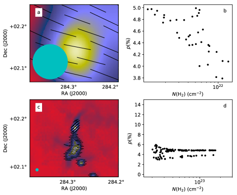
Figure 18: Predictions of the toy magnetic field model with constant grain alignment. The polarisation vectors are shown on the column density map in frame a (central part of the full map) and the $p$ vs. $N({\rm H}_{2})$ relation is plotted in frame b at Planck resolution. The lower frames are the same for synthetic POL-2 observations, at a resolution of 20$\arcsec$, assuming high-pass filtering with $\theta=200\arcsec$. The scaling of the absolute $p$ values is arbitrary but identical between the frames.

Figure 19: Same as Fig. 18 but using grain alignment predicted by RAT calculations. In frame d, the red points correspond to data with spatial high-pass filtering with a scale of $\theta=100\arcsec$ instead of the default value of $\theta=200\arcsec$.

Figure 20: The same model with RAT alignment as in Fig. 19 but assuming a factor of two larger grain sizes.

When the alignment predicted by RAT is taken into account (Fig. 19), the POL-2 polarisation fractions drop below the Planck values but now the Planck values show an even slightly stronger dependence on column density, in contrast with the observations of the G035.39-00.33 field. Figure 19d shows $p$ vs. $N({\rm H}_{2})$ also for a POL-2 simulation where the data are assumed to be high-pass filtered at a scale of $\theta=100\arcsec$ instead of $\theta=200\arcsec$. The different filtering does not have a strong effect but leads to some larger values towards the edges of the filament.

The RAT calculations of Fig. 19 were not completely self-consistent because they employed the original grain size distributions (see Sect. 3.3) while assuming an increased dust opacity at sub-millimetre wavelengths. We made an alternative simulation where the grain alignment (and thus the polarisation reduction factor) was calculated assuming a factor of two larger grains. The comparison of these results in Fig. 20 with the previous calculations of Fig. 19 should partly quantify the uncertainty associated with the particle sizes. A factor of two change in the grain size in first approximation corresponds to a factor of two increase in the POL-2 polarisation fractions. The effect on the simulated Planck observations is small, because most grains were already aligned outside the dense filament. For RAT alignment with the larger grain sizes, Appendix D shows results for an alternative model where the POS magnetic field orientations are taken from POL-2 observations (at 20$\arcsec$ resolution) for the model volume with $n({\rm H}_{2})>3\times 10^{3}$ cm^-3. There the polarisation fractions are on average lower only by a fraction of a percent. The difference is larger in the northern clump, which is sensitive to changes in the magnetic field configuration, probably because of the stronger geometrical depolarisation that results from the orthogonality of the local and the extended fields.

Figure 21 compares the constant alignment and RAT cases to models where $R$ has an ad hoc dependence on the volume density. The grains are perfectly aligned at low densities but $R$ decreases smoothly to zero above a density threshold $n_{0}$,

$$R=0.5+0.5\tanh\left[\log_{\rm 10}(n_{0})-\log_{\rm 10}(n)\right].$$ (15)

In the modelling the absolute scale of $p$ is left free. In Fig. 21 the values are scaled so that the Planck polarisation fraction is $2.5\%$ or have a maximum value of 3% in the case of the $n_{0}$ dependence. The only real constraint is provided by the ratio of the Planck and POL-2 polarisation fractions. The observed ratio $\sim 2.5$ is reached for a density threshold of $n_{0}=10^{4}$ cm^-3. The constant-alignment model predicts a smaller ratio while the initial RAT model gives a higher ratio. However, if RAT calculation assume a factor of two larger grain sizes, the ratio falls slightly below the observed value.

Finally, we also examined models where the dust opacity ratio was $\tau(250\mu{\rm m})/\tau({\rm J})=1.0\times 10^{-3}$. The lower sub-millimetre opacity means that the modelling of surface brightness data led to larger volume densities and to a lower radiation field intensity inside the cloud. Both factors contribute to a lower grain alignment in RAT calculations (see Eq. 14). In Fig. 21 the change from $\tau(250\mu{\rm m})/\tau({\rm J})=1.6\times 10^{-3}$ to $\tau(250\mu{\rm m})/\tau({\rm J})=1.0\times 10^{-3}$ increases the ratio of Planck and POL-2 polarisation fractions by over 30%.

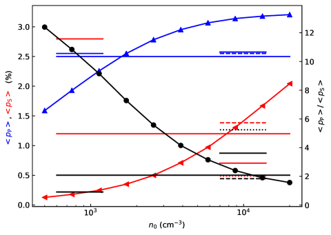
Figure 21: Polarisation fractions for different grain alignment models. The long horizontal lines show the observed average values of $p$ (left y-axis) for the Planck ($p_{\rm P}$, blue line) and the POL-2 ($p_{\rm S}$, red line) observations. The black long horizontal line stands for the observed $\langle p_{\rm P}\rangle/\langle p_{\rm S}\rangle$ ratio (right y-axis). The three curves with markers show the corresponding quantities for models that assume a loss of grain alignment above the density threshold $n_{0}$. The results for models with constant grain alignment are indicated with short horizontal lines near $n=10^{3}\,{\rm cm}^{-3}$. The RAT models are shown as short horizontal lines near $n=10^{4}\,{\rm cm}^{-3}$, for the default model (solid lines), for the case with larger grain sizes (dashed line), and for an alternative model with a smaller $\tau(250\mu{\rm m})/\tau({\rm J})$ ratio (dotted line).

Unfortunately the observed $p$ ratio does not provide strong constraints on the grain alignment because the quantitative results also depend on the assumed magnetic field geometry. As an example, we tested a field configuration where the southern filament has a toroidal field at densities above $n=3\times 10^{3}$ cm^-3 while the field in the northern part is still uniform (poloidal). A toroidal field is consistent with the observed magnetic field orientation that is perpendicular to the southern filament. Regarding the $p$ vs. $N$ relation, it is also an interesting special case that results in stronger geometrical depolarisation as one moves away from the symmetry axis. The results for the constant alignment and an RAT alignment models are shown in Figs. 22-23. In the constant alignment case the Planck polarisation fractions have not changed but the POL-2 values show a larger scatter and a lower average polarisation fraction. At the borders of the filament, where the toroidal field of is along the LOS in the dense medium, the polarisation vectors have turned parallel to the large-scale field. The change is qualitatively similar for the RAT case (Fig. 23). The $p$ vs. $N$ relation is flatter than in Fig. 19 but not significantly different from the observations shown in Fig. 14b. In the model the toroidal configuration also causes a stronger drop in the $Planck$-observed polarisation fraction. A more extended toroidal component (e.g. in a test where the density threshold was reduced from $n=3\times 10^{3}$ cm^-3 to $n=5\times 10^{2}$ cm^-3) would cause clear changes also in the orientation of the $Planck$-detected polarisation vectors. However, these effects are dependent on our assumptions of the LOS matter distribution and would disappear if most of the extended material was located far from the filament.

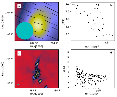
Figure 22: Same as the constant alignment case of Fig. 18 but assuming a toroidal field for the southern clump.

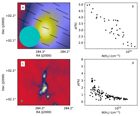
Figure 23: Same as the RAT alignment case of Fig. 19 but assuming a toroidal field for the southern clump.

6 Discussion

In the following we discuss the results regarding the observable dust properties (Sect. 6.1) and the polarisation fraction(Sect. 6.2).

6.1 Dust opacity in the G035.39-00.33 field

The G035.39-00.33 field has a high-column-density background of $N({\rm H}_{2})\sim 10^{22}$ cm^-2 (Fig. 3). Even after the subtraction of this background, the column densities are above $N({\rm H}_{2})=2\times 10^{22}$ cm^-2 over a filament length of $\sim 7\arcmin$ ($\sim$6 pc). With a typical filament width of $\sim 40\arcsec$, the average volume density is of the order of $n({\rm H}_{2})\sim 10^{4}$ cm^-3. With the high volume density and the dust temperatures below 14 K (with minima close to $T=12$ K, see Sect. 4.1-4.2), the conditions are suitable for grain evolution. The properties of dust opacity can thus be expected to be different from those of diffuse clouds.

The comparison of dust sub-millimetre emission and NIR/MIR observations gave an average opacity ratio of $\tau(250\mu{\rm m})/\tau({\rm J})=(2.55\pm 0.03)\times 10^{-3}$, which also is close to the behaviour of the southern clump. The relation is steeper in the northern clump, although only in small $\sim 1\arcmin$ region that is close to some 70 $\mu$m sources. Internal heating could reduce the degree to which dust optical depth $\tau(250\,\mu{\rm m})$ is underestimated. The fit at $\tau({\rm J})<$6 gave a lower value of $\tau(250\mu{\rm m})/\tau({\rm J})=(1.72\pm 0.04)\times 10^{-3}$. In the RT models, $\tau({\rm J})\sim 6$ ($\tau(250\,\mu{\rm m})\sim 0.012$) typically corresponds to a LOS peak volume density of the order of $n({\rm H_{2}})=5\times 10^{3}$ cm^-3. Planck studies have found in diffuse regions values $\tau(250\,\mu{\rm m})/N({\rm H})\sim 0.55\times 10^{-25}$ cm² H^-1 (Planck Collaboration XI 2014; Planck Collaboration Int. XVII 2014). With the Bohlin et al. (1978) relation between the reddening and Hydrogen column density and with the $R_{\rm V}=3.1$ extinction curve (Cardelli et al. 1989), this corresponds to $\tau(250\mu{\rm m})/\tau({\rm J})=0.41\times 10^{-3}$. The G035.39-00.33 sub-millimetre opacity values relative to NIR are thus more than four times higher than in diffuse clouds.

The correlation between density and sub-millimetre opacity is known from numerous studies (Kramer et al. 2003; Stepnik et al. 2003; Lehtinen et al. 2004; del Burgo & Laureijs 2005; Ridderstad & Juvela 2010; Bernard et al. 2010; Suutarinen et al. 2013; Ysard et al. 2013; Martin et al. 2012; Roy et al. 2013; Svoboda et al. 2016; Webb et al. 2017). Juvela et al. (2015c) used Herschel observations to study sources from the Planck Catalogue of Galactic Cold Clumps (PGCC, Planck Collaboration et al. 2016). For a sample of 23 fields the average dust opacity was $\tau(250\mu{\rm m})/\tau({\rm J})=1.6\times 10^{-3}$. Given that this value corresponds to sources with optical depths below $\tau({\rm J})\sim 3$, it is in qualitative agreement with the results of the present study. In Juvela et al. (2015c), the maximum values derived for individual clumps were $\tau(250\mu{\rm m})/\tau({\rm J})=4\times 10^{-3}$, similar to the value of the northern clump of G035.39-00.33 . However, in that study the NIR extinction estimates were based on background stars only and, in the case of high optical depths, have a higher uncertainty.

A large $\tau(250\,\mu{\rm m})/\tau({\rm J})$ ratio also could result from an underestimation of the $\tau({\rm J})$ values in the G035.39-00.33 field. The lack of background stars should not directly affect the $\tau({\rm J})$ estimates of the densest filament, which are based more on MIR data but if the MIR emission had a strong foreground component, that could also lead to low $\tau({\rm J})$ estimates. he uncertainty of extinction depends non-linearly on the foreground intensity but it is probably only some 10-20% (see also Butler & Tan 2012b). In the analysis of Kainulainen & Tan (2013), the MIR extinction also was tied to the NIR extinction measurements, which makes large errors in the extinction levels improbable. Even with an uncertainty of 30% (see Kainulainen & Tan 2013), the 1-$\sigma$ lower limit is still above the average value of Juvela et al. (2015c).

The estimates of the sub-millimetre opacity $\tau(250\,\mu{\rm m})$ are likely to be biased because they were derived from single-temperature MBB fits, ignoring the effects of LOS temperature variations. Figure 17 compared the true column densities of a model cloud to those derived from the synthetic surface brightness maps. This also serves as an estimate for the bias of the $\tau(250\,\mu{\rm m})$ values. At a column density of $N({\rm H}_{2})=10^{23}$ cm^-2 the estimated bias is more than a factor of two. This column density is higher than the values $N({\rm H}_{2})\la 5\times 10^{22}$ cm^-2 estimated for G035.39-00.33 . However, these are consistent if the latter are underestimated by the factor indicated by the modelling. Quantitatively the bias predictions depend on how well the models represent the real cloud. A stronger internal heating would decrease the bias, at least locally. Conversely, the observations do not give strong constraints on the maximum (column) densities and higher optical depths would lead to a higher bias. The relative bias is likely to be at least as large in $\tau(250\,\mu{\rm m})$ as in $\tau({\rm J})$. Thus, the true value of $\tau(250\mu{\rm m})/\tau({\rm J})$ may be even higher than the quoted estimate of $2.55\times 10^{-3}$.

The calculation of the sub-millimetre opacity assumed a fixed dust opacity spectral index of $\beta=1.8$, which is close to the spectral index estimated from the data (see below). An error of $\sim 0.1$ in the spectral index would correspond only to $\sim$10% error in opacity. For further discussion of the effect of the spectral index and the extinction law, see Juvela et al. (2015c). Finally, if the actual resolution of our $\tau_{\rm 5}(250\,\mu{\rm m})$ map were lower than the nominal 15$\arcsec$, this would lower the $\tau(250\,\mu{\rm m})/\tau({\rm J})$ estimates. When the maps were convolved to a lower resolution with a Gaussian beam with FWHM=$20\arcsec$, the opacity ratio changed by less than 0.03 units. This shows that the result is not sensitive to the resolution.

We estimated a dust opacity spectral index of $\beta\sim 1.9$ for the main G035.39-00.33 filament, using data at $\lambda\leq 850\,\mu$m. For the northern part separately, the $\beta$ values were slightly lower but there both the SCUBA-2 450 $\mu$m and 850 $\mu$m values were above the relation fitted to SPIRE data (Fig. 5). These offsets and thus the lower $\beta$ values could be caused by uncertainties in the spatial filtering or, when using background-subtracted data, the reference region being located at a larger distance in the south (see Fig. 1b).

The derived $\beta$ value is practically identical to the median value $\beta=1.91$ that Juvela et al. (2015a) reported for a sample of GCC clumps based on Herschel data with $\lambda\leq 500\,\mu$m. In Juvela et al. (2015b) the inclusion of longer wavelength Planck data resulted in a smaller value of $\beta=1.66$. This wavelength-dependence had been demonstrated, for example, in Planck Collaboration Int. XIV (2014). More recently, Juvela et al. (2018) analysed Herschel and SCUBA-2 observations of cores and clumps within some 90 PGCC fields. For those objects the median value at Herschel wavelengths was $\beta\sim 1.8$ (although with significant scatter) and the inclusion of the SCUBA-2 850 $\mu$m data point decreased the value closer to $\beta\sim 1.6$. The higher spectral index value of the G035.39-00.33 field is again in qualitative agreement with G035.39-00.33 being more dense and, in terms of dust evolution, probably a more evolved region. Spectral indices are generally observed to be higher towards the end of the prestellar phase while in the protostellar phase one may again observe lower values (Chen et al. 2016b; Li et al. 2017; Bracco et al. 2017). This may be caused by dust evolution (e.g. further grain growth), by the temperature variations resulting from internal heating, or directly by problems associated with the analysis of observations at very high column densities (Shetty et al. 2009b, a; Juvela & Ysard 2012a; Malinen et al. 2011; Juvela & Ysard 2012b; Ysard et al. 2012; Juvela et al. 2013b; Pagani et al. 2015). The G035.39-00.33 field does contain a number of protostellar objects but in this paper we only examined the average $\beta$ over the whole filament.

6.2 Polarisation

The polarisation observations trace a combination of magnetic field morphology and grain properties. Planck and POL-2 provided different views into the structure of the magnetic fields. The large-scale field was found to be uniform while the small-scale structure associated with the dense filament was more varied, even with partly orthogonal orientations. The Planck and POL-2 data are not contradictory because of the large difference in the beam sizes. POL-2 also is not sensitive to the extended emission (Sect. 4.5). Nevertheless, the change in the field orientations must be constrained to a narrow region at and around the main filament. Otherwise these would be visible also in Planck data, as deviations from the average field orientation and as a reduced net polarisation. If connected to the gravitational instability of the filament and of the embedded cores, the effects are naturally confined in space. If strong accretion flows extend to a distance of $\sim$1 pc, this corresponds to only $\sim 1\arcmin$ in angular distance.

In the following we discuss in more detail the observations and the modelling of the polarisation fraction.

6.2.1 Observed polarisation fractions

The polarisation fraction $p$ is generally observed to decrease towards dense clouds and especially towards dense (prestellar) clumps and cores (Vrba et al. 1976; Gerakines et al. 1995; Ward-Thompson et al. 2000; Alves et al. 2014; Planck Collaboration Int. XX 2015; Planck Collaboration Int. XXXIII 2016).

The Planck data were used to characterise the large-scale environment of the G035.39-00.33 filament. Planck data did not show any clear column density dependence over the examined $2\degr\times 2\degr$ area and the bias-corrected polarisation fraction estimate $p_{\rm mas}$ remained within a narrow range between 1% and 3% (Fig. 12). The same was already evident based on the polarisation vectors that were plotted in Fig. 10a. These show that the large-scale magnetic field orientation is very uniform, also in the area covered by POL-2 observations. The dynamical range of column density over this area was only a factor of $\sim$3, which partly explains the lack of a clear correlation. The polarised signal is largely dominated by extended emission not directly connected to the dense filament. Because of the low Galactic latitude, there can be contributions from many regions along the LOS, which would tend to decrease the observed polarisation fraction (Jones et al. 1992; Planck Collaboration Int. XIX 2015). In Liu et al. (2018b), multiple velocity components were identified from ¹³CO and C¹⁸O line data. Only the 45 km s^-1 feature, the strongest of the kinematic components, is associated with the main filament. This is consistent with the picture shown by Fig. 1a and Fig. 3. At Herschel resolution the filament rises more than a factor of four above the extended column density background while at the Planck resolution it is associated with a mere 50% increase above the background surface brightness. With the added effect of spatial filtering, POL-2 measurements are only sensitive to the emission from the main filament. Conversely, Planck measurement could be slightly affected by the dense filament, unless that is associated with lower polarisation fractions.

The uniformity of the magnetic field is shown quantitatively by the polarisation angle dispersion function $S$ calculated from the Planck data. Figure 13c showed the relation $\log\,p=-0.670\,\log\,S-0.97$ that Fissel et al. (2016) derived from BLASTPol observations of the Vela C molecular cloud (“ISRF-heated sightlines”). Compared to this, the Planck data of the G035.39-00.33 field indicate much lower ($p$, $S$) parameter combinations. Figure 13c also included the relation $\log_{10}(S)=-0.834\times\log_{10}(p_{\rm mas})-0.504$ that Planck Collaboration Int. XIX (2015) obtained at larger scales (FWHM=$1\degr$, $\delta=30\arcmin$), using data over a large fraction of the whole sky. This relation corresponds to higher values of $S$ and $p$ than found in the G035.39-00.33 field. The comparison to the Planck results (Planck Collaboration Int. XIX 2015) is not straightforward because observations probe different linear scales (FWHM=1$\degr$ compared to FWHM=$9-15\arcmin$ in our analysis). Figure 13 did not show a systematic dependence on the scale. Planck Collaboration XII (2018) detected a shallow relation of $S\times p\propto FWHM^{0.18}$, which would thus be detectable only by using a wider range of scales. According to that relation, the $S\times p$ values at 15$\arcmin$ resolution should be only some 22% smaller than at 1$\degr$ resolution.

Instead of grain alignment or the statistical averaging of LOS emission with different polarisation angles), lower G035.39-00.33 polarisation fractions (in relation to $S$) could be explained by a larger LOS component of the magnetic field, a hypothesis that we cannot directly test. Large angles between the magnetic field and the POS would tend to be associated with large values of $S$ (Chen et al. 2016a). However, this is only a statistical correlation and cannot be used to exclude the possibility of a large LOS field component, which also would be consistent with the Galactic longitude and distance of the G035.39-00.33 field.

Compared to the low-resolution Planck data, the POL-2 data are more affected by observational noise. The bias-corrected polarisation fraction estimates $p_{\rm mas}$ are reliable for the central filament and are there $p_{\rm mas}\sim 1\%$ irrespective of the data resolution between FWHM=$15\arcsec$ and FWHM=$60\arcsec$ (see Fig. 34).

The POL-2 $p_{\rm mas}$ estimates should be unbiased when used at 40$\arcsec$ resolution and when the analysis is restricted to column densities $N({\rm H}_{2})>2\times 10^{22}$ cm^-2. In this range, the decrease of polarisation fraction as a function of column density is significant (Fig. 14). The drop from $N({\rm H}_{2})=2\times 10^{22}$ cm^-2 to $N({\rm H}_{2})=4\times 10^{22}$ cm^-2 is from 1.5% to values below 1%. Because low-density regions along the LOS (in front of and behind the filament but possibly associated to it) will produce some polarised intensity, a non-zero polarisation fraction does not exclude the possibility of a complete loss of grain alignment within the densest filament.

The simulations presented in Appendix C confirm that the negative correlation between $p_{\rm mas}$ and $N({\rm H}_{2})$ is larger than expected based on the noise alone (Fig. 36). These also show that with column densities $N({\rm H}_{2})>10^{22}$ cm^-2 and with FWHM$>20\arcsec$ most of the resolution dependence of $p$ can be attributed to geometrical depolarisation (Fig. 37). This is related to the $S$ function. Planck data showed some anticorrelation between $p_{\rm mas}$ and $S$ (Fig. 8) but this dependence was not clear in POL-2 data. While Fig. 11 gave some indications, especially in the northern part, statistically the anticorrelation remained weak (Fig. 15d). Reliable mapping of $S$ would require higher SNR further out from the central filament. On the other hand, $S$ also is also affected by the filtering of the extended emission.

Because polarisation fraction is correlated with column density, it could be expected to be correlated with tracers of dust evolution such as $\tau(250\mu{\rm m})/\tau({\rm J})$. However, physically high volume density should be associated with grain growth, which in turn works against drop of polarisation that in the RAT scenario is caused by the weakening of the radiation field. Figure 24 shows no clear correlation between $p_{\rm mas}$ and the opacity ratio $\tau(250\mu{\rm m})/\tau({\rm J})$ and only the correlation between $\tau(250\mu{\rm m})/\tau({\rm J})$ and $N({\rm H}_{2})$ is significant (correlation coefficient $r=0.45$, significant at $\sim 98\%$ level when calculated with data sampled at FWHM steps). As mentioned in Sect. 4.6.2, 70 $\mu$m sources tend to have lower than average polarisation fractions, in this sample 1.1% vs. 1.4%. Part of this is caused by their higher SNR and thus lower bias, although for the data in Fig. 24 the bias should not be very significant.

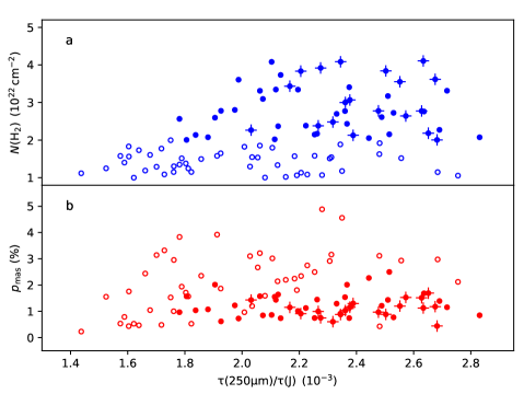
Figure 24: Correlations between opacity ratio $\tau(250\mu{\rm})/\tau({\rm J})$ and column density (frame a) or POL-2 polarisation fraction (frame b). The data are at 40$\arcsec$ resolution and sampled at half-beam steps. The points coinciding with the point sources marked in Fig. 14 are marked with plus signs. Data for column densities $N({\rm H}_{2})<2\times 10^{22}\,{\rm cm}^{-2}$ are plotted with open symbols and for these the $p_{\rm mas}$ estimates may be inaccurate.

6.2.2 Simulations of polarised emission

We used RT simulations to probe the effects that magnetic field geometry and grain alignment variations can have on the polarisation observations. Because the absolute values of the polarised intensity depend on poorly known grain properties, small-scale magnetic field structure, and the strength of the LOS magnetic field component, we concentrated on the ratio of the simulated Planck and POL-2 polarisation fractions.

In the case of constant grain alignment, the polarisation fractions were even higher in the simulated POL-2 data than in the simulated Planck data (Fig 18), in clear contradiction with observations. When grain alignment was assumed to depend on volume density, the ratio of Planck and POL-2 polarisation fractions could be matched with a density threshold of $n({\rm H}_{2})=10^{4}$ cm^-3. This can be compared to Alves et al. (2014) (see also Alves et al. 2015), who analysed optical, NIR, and sub-millimetre observations of a starless core in the Pipe nebula. They deduced a loss of alignment at densities $n({\rm H}_{2})>6\times 10^{4}$ cm^-3. The analyses are of course affected by many uncertainties (see Sect. 6.2.3) and, because of the larger distance, the linear resolution of our observations is much lower. If the difference in the density thresholds were significant, it could be related to the different nature of the sources (e.g. evolutionary stage and internal heating).

The low $p$ values of the actual G035.39-00.33 observations could be explained by geometrical depolarisation resulting from line tangling within the densest filament. However, this does not seem a likely explanation given the local uniformity of the polarisation angles and the relatively constant polarisation fraction observed over the whole filament. The synthetic Planck $p$ values also dropped by $\sim$30% as a function of column density (Fig. 18b), while in the actual observations no clear column-density dependence was seen (Fig. 12c). However, our models described only a $13\arcmin\times 13\arcmin$ area and a volume of $\sim(11\,{\rm pc})^{3}$. About half of the actual Planck signal is coming from a more extended cloud component (cf. Fig 1a-b) that appears to be associated with at least a factor of two higher polarisation fractions than the main filament. If the extended component was added, the $p$ values would not change at low column densities while the values towards the filament would increase significantly. Therefore, the $p$ vs. $N$ relation of the simulated Planck observations is not necessarily incompatible with the observations. A more remote possibility for such $p$ vs. $N$ relations would be to assume that the direction of the large-scale field is changing so that (unlike in simulations) it has a larger LOS component in the low-column-density regions (cf. Planck Collaboration Int. XXXIII 2016).

Figure 19 showed the results for a model where the grain alignment efficiency varied as predicted by RAT. In the synthetic Planck data the polarisation angles were again uniform, similar to the real G035.39-00.33 observation. The simulated POL-2 polarisation fractions were too low compared to the Planck values outside the filament. The discrepancy could be corrected by using a factor of two larger grains in the alignment calculations (Fig. 20). The observed high sub-millimetre opacity indicates some grain growth, which, however, is unlikely to be as large as a factor of two. In reality, the effects of grain growth are more complex because also the grain shapes are probably affected.

In the more empirical modelling we simply assumed that grain alignment is lost above a certain volume density. The observed ratio of polarisation fractions was recovered when the threshold was $n({\rm H}_{2})\sim 10^{4}$ cm^-3. This would thus be consistent with no polarised intensity being emitted from the densest filament. The differences between the large-scale and the small-scale field morphologies would thus only probe the envelopes of the filament and the cores embedded within the filament (Appendix D).

6.2.3 Uncertainties of polarisation simulations

There are several caveats concerning the polarisation simulations and the comparison with the Planck and POL-2 observations.

In the modelling, the filtering of the POL-2 data was described using a simple high-pass filter. Figure 19 showed that the difference between filtering scales $\theta=100\arcsec$ and $\theta=200\arcsec$ was not significant. This is understandable because any high-pass filtering with a scale larger than the filament width will effectively remove all information of the uniform large-scale field. However, the actual filtering in POL-2 data reduction is not necessarily this simple. One needs simulations with the actual POL-2 reduction pipeline, to estimate the general effect of the filtering and to check for potential differences in the way the different Stokes vector components get processed.

The minimum size of the aligned grains and thus the polarisation reduction associated to RAT was calculated for the original grain size distributions of Compiègne et al. (2011) while the sub-millimetre emissivity was subsequently altered (see Sect. 3.3). A subsequent factor of two increase of the grain sizes had no effect on the simulated Planck values but increased the POL-2 polarisation fraction by $\sim$30%. The total uncertainty related to the grain properties could be higher. The results depend not only on the grain size distribution but also on other poorly known factors that are related to the grain composition, grain shapes, and optical properties. Rather than an indication of specific dust opacities or grain sizes, the model comparison in Fig. 21 should only be taken as an indication of some of the uncertainties that affect the modelling of polarised dust emission.

Our models did not consider the effect of internal heating sources. While young stellar objects (YSOs) increase the radiation flux in their environment, this does not necessarily lead to significant enhancement of the observed polarisation. The angular momentum caused by the radiation reaches its maximum when radiation direction is aligned with the magnetic field (Hoang & Lazarian 2009). If the grain’s angular momentum $J$ is aligned with the magnetic field, only the RAT component projected onto the magnetic field direction is able to spin up the grain, leading to Eq. (38) of Hoang & Lazarian (2014): $J^{\rm RAT}_{\rm max}(\psi)=J^{\rm RAT}_{\rm max}(\psi=0)\cos\psi$. If the aligning radiation is directed towards the observer, the angular momentum reaches its maximum when also the magnetic field is parallel to the observer’s LOS. This leads to strong depolarisation thanks to the $\cos^{2}\gamma$ term. On the other hand, for $\cos^{2}\gamma=1$, $\cos\psi=0$ and hence collisions are able to disrupt the grain alignment. Since RATs are effective mostly at UV and optical wavelengths, deeply embedded and already reddened YSOs may have an effect only in their immediate surroundings, which may correspond to a small part of the total dust along the LOS. Combined with the large beams of the sub-mm telescopes, the contribution of YSOs on the polarisation of distant clouds may thus remain negligible.

The comparison of the simulated Planck and POL-2 observations assumed that Planck is able to give an upper limit for the intrinsic polarisation. If the magnetic field had a strong random component, the $p_{\rm P}$ values observed with the large Planck beam would however underestimate this maximum polarisation fraction. Conversely, if line tangling were confined to the filament, a possibility also not probed by our models, this would lead to lower $p$ in POL-2 observations. However, the RAT simulations appear to leave little room for additional geometrical depolarisation within the filament.

For the most part, our simulations assumed that the LOS magnetic field component is constant and similar both at large scales and within the filament. The ratio of the Planck and POL-2 values $p_{\rm P}/p_{\rm S}$ would be lower if the LOS field component was systematically larger outside the filament. For example, the large-scale field could be at 45 degree angles relative to the LOS while a toroidal field in the filament would make the field more perpendicular to the LOS towards the filament centre. Because the polarised intensity is proportional to $\cos^{2}\gamma$, the effect on the $p_{\rm P}/p_{\rm S}$ ratio would be a factor of two. The effect would be quite significant and, if it were true, would even more strongly point to a complete loss of grain alignment inside the filament. Of course, the opposite situation where the field outside the filament is more closely aligned with the POS is in principle also possible.

The dust temperatures obtained from RT calculations contain some Monte Carlo noise but, once the temperature field is fixed, the $I$, $Q$, and $U$ maps are mutually consistent to a very high accuracy. The simulated $p$ values do not therefore suffer from noise bias but there are other uncertainties that are related to the underlying RT model. The intensity and the spectrum of the radiation field at the boundaries of the model volume affect especially the RAT calculations. Different assumptions of the dust sub-millimetre opacity were already seen to lead to models with different column densities and, consequently, different internal radiation fields. In Fig. 21, compared to the RT model with $\tau(250\mu{\rm m})/\tau({\rm J})=1.6\times 10^{-3}$, the assumption of $\tau(250\mu{\rm m})/\tau({\rm J})=1.0\times 10^{-3}$ lead to a 30% higher ratio of the Planck and POL-2 polarisation fractions. The continuum observations also do not give strong constraints on the volume densities. If we assumed the cloud to be more extended in the LOS direction, this would decrease the volume density and increase the short-wavelength radiation inside the cloud. Both factors would enhance grain alignment (see Eq. (14)). An inhomogeneous cloud structure would increase the penetration of the external radiation but this would be partly compensated by the larger volume densities.

The best way to combat many of the listed uncertainties would be to study large samples of sources and use statistical arguments regarding the field orientation and the cloud shapes.

6.3 Field geometry vs. grain alignment

Planck studies have concluded that at large scales the relation between polarisation fraction $p$ and column density $N$ can be explained by the structure of the magnetic field without variations in the grain alignment. Planck Collaboration Int. XX (2015) found that the $p(N)$ relation was fairly well reproduced by MHD simulations with constant grain alignment but their observations only probed column densities up to $N({\rm H}_{2})=5\times 10^{21}$ cm^-2. They refrained from drawing any conclusions for high column densities $N({\rm H}_{2})>10^{22}$ cm^-2 for which also their MHD runs were not well suited. Soler et al. (2016) similarly concluded that at $N({\rm H}_{2})<5\times 10^{21}$ cm^-2 the polarisation angle dispersion and its relation to the polarisation fraction were mainly produced by fluctuations in the magnetic field structure.

Planck Collaboration XII (2018) examined in more detail the relationships between $p$, $N$, and $S$. The uniformity of the product $p\times S$ was noted as evidence that the drop in $p(N)$ is caused by the field structure rather than a loss of grain alignment. At a resolution of 40$\arcmin$, the $p(N)$ relation of Gould Belt clouds was followed up to $N({\rm H}_{2})=5\times 10^{21}$ cm^-2. The probed linear scales were thus $\sim$1.6 pc for nearby clouds and $\sim$5 pc for Orion. The column densities are low because of the spatial resolution, which means that even towards the densest structures the polarised signal may be strongly affected by extended emission (usually with a higher polarisation fraction). However, with data at 10$\arcmin$ resolution, Planck Collaboration XII (2018) Fig. 21 traces the product $p\times S$ up to $N({\rm H}_{2})=10^{23}$ cm^-2. The reduction of the grain alignment efficiency was estimated to be less than 25% between the diffuse ISM and the highest column densities. However, even at the highest column densities the data do not exclusively probe the emission from regions of high volume density. Some drop in $p\times S$ was observed beyond $N({\rm H}_{2})\sim 3\times 10^{22}$ cm^-2. This was not very significant but, in principle, could hint at effects of reduced grain alignment being visible even in Planck data. Alternatively, this could be related to a qualitative change in the field morphology at scales dominated by the gravity.

These results are not directly comparable to our POL-2 study of the massive filament G035.39-00.33. Even with the higher angular resolution of POL-2 (0.56 pc for the 40$\arcsec$ angular resolution and the 2.9 kpc distance) the filament is not fully resolved. However, the observed column densities, $N({\rm H}_{2})>10^{22}$ cm^-2, and especially the volume densities are much higher than what is reached with Planck . Planck Collaboration Int. XX (2015) concluded that large column densities can be associated to low polarisation fraction especially because of the accumulation of many LOS structures. Our POL-2 observations target a single object that dominates the LOS column density. All extended emission also is already filtered out from the POL-2 data. For G035.39-00.33, the difference to the Planck data of the same region is particularly striking because of the low Galactic latitude (see Fig. 1).

Planck studies concluded was that their observations are consistent with constant grain alignment. Similarly, based on the POL-2 data and radiative transfer simulations, we can conclude that the observed $p(N)$ drop can be explained by the RAT mechanism alone, which even tends to overestimate the drop in $p$. The two conclusions are not necessarily contradictory. First, they apply to different parts of the ISM, POL-2 probing a source of much higher volume density. Second, the magnetic field geometry remains a significant source of uncertainty in our modelling and we cannot put a strict upper limit on its effects. For a single source, almost any $p(N)$ relation can be explained with a suitably crafted field geometry (small-scale structure or changes in the orientation relative to the LOS), without a need for variations in the grain alignment efficiency.

Another point of comparison is provided by the recent NIR polarimetry of the starless core FeSt 1-457 presented by Kandori et al. (2018). They did not observe any (significant) drop in the polarisation efficiency up to column densities of $A_{\rm V}\sim 20$ mag. This is qualitatively in contradiction with the RAT predictions, although the authors noted that grain growth could provide at least a partial explanation. Furthermore, based on the extinction data discussed in Sect. 2.4, the extinction in the G035.39-00.33 field reaches significantly higher values. These are some $A_{\rm V}\sim 50$ mag in both the northern and the southern clump, when measured at a resolution of 15$\arcsec$. Indeed, the comparison of a set of NIR and submm polarisation observations lead Jones et al. (2015) to conclude that grain alignment is lost around $A_{\rm V}\sim 20$ mag.

It is clear that even if grain alignment is partially lost, also the magnetic field orientation is never uniform and thus has some effect on the polarisation observations. To determine the relative importance of the two factors, we need more comparisons of high-resolution observations and simulations.

7 Conclusions

We have used Planck, Herschel, and SCUBA-2/POL-2 data to investigate dust emission and sub-millimetre polarisation in the G035.39-00.33 field. Our main conclusions are the following:

The $\sim$6 pc long main filament of the G035.39-00.33 field is characterised by dust colour temperatures $T\sim 12-14$ K and a column density in excess of $N({\rm H}_{2})=2\times 10^{22}$ cm^-2.

The average sub-millimetre to NIR dust opacity ratio of the filament is $\tau(250\mu{\rm m})/\tau({\rm J})=(2.55\pm 0.03)\times 10^{-3}$. This is more than four times higher than in diffuse clouds and slightly higher than for previous samples of PGCC clumps of lower column density.

The average dust opacity spectral index of the filament is $\beta\sim 1.9$. This is similar to the values that previous studies have found for larger samples of PGCC clumps.

At large scales, Planck data show a relatively uniform magnetic field orientation but a polarisation fraction of only $p\sim$2%. The values of the polarisation angle dispersion function are on average $S(\delta\sim 2.5\arcmin)\sim 9\degr$ and only slightly lower at the location of the G035.39-00.33 filament. The $S(p)$ relation was examined at resolutions between FWHM=$5\arcmin$ and FWHM=$15\arcmin$ and was found to be between the Planck Collaboration Int. XIX (2015) results (obtained at much larger scales) and a lower $S=0.1/p$ relation.

POL-2 data reveal a very low polarisation fraction of $p\sim 1\%$ for the densest filament. The negative correlation between the polarisation fraction and column density is significant at $N({\rm H}_{2})>2\times 10^{22}$ cm^-2.

Observations are consistent with models with an almost complete loss of grain alignment at densities above $n({\rm H}_{2})\sim 10^{4}$ cm^-3. RAT calculations overestimate the decrease of polarised intensity, although this can be corrected by assuming a strong increase in grain sizes (a factor of two). The modelling is affected by large uncertainties in the grain properties, the magnetic field geometry (including the small-scale structure and the average LOS field component), and the underlying physical cloud model. Therefore, the relative importance of grain alignment and field geometry for the $p(N)$ relation remains open. High-resolution polarisation observations of a statistically significant sample of filaments, clumps, and cores are needed.

Appendix A Modified blackbody fit to maps of different resolution

Section 3.1 described how column density can be estimated using surface brightness maps that are first convolved down to a common resolution. The resolution can be increased in several ways. Palmeirim et al. (2013) employed different combinations of the observed bands. All bands were first used to derive a column density map $N_{0}$ at the lowest common resolution. The lowest resolution bands are then removed one by one and the remaining bands are used to calculate corrections for higher spatial frequencies. On each step a new map is obtained as

$${\hat{N}_{i}}={\hat{N}}_{i-1}+{\rm HPF}(N_{i},{\rm FWHM}_{i-1}),$$ (16)

where ${\hat{N}}_{i-1}$ is the previous estimate at the resolution ${\rm FWHM}_{i-1}$. $N_{i}$ is a resolution ${\rm FWHM}_{i}$ map that is calculated using the maps that have a resolution better or equal to ${\rm FWHM}_{i}$, all convolved to ${\rm FWHM}_{i}$). HPF stands for high-pass filtering for the indicated beam size. In the following, we refer to this as method A.

In Sect. 4.1 we made high-resolution column density maps by constructing a model that consisted of high-resolution maps of temperature and surface brightness at a reference frequency. The model was optimised by comparing its predictions with the observed surface brightness maps, each at its original resolution. This procedure (in the following method B) is time-consuming because each optimisation step involves convolutions. The model parameters also are not independent between pixels and must be solved simultaneously. After optimisation, the model maps can be converted to a column density map. The nominal resolution could be even higher than in method A but regularisation may be needed to avoid oscillations that are typical for deconvolution. The pixel size of the model maps must be small compared to the resolution of the observations. In Sect. 4.1, the best resolution of observations was 18$\arcsec$, the model was defined 6$\arcsec$ pixels, and the final result was at a resolution of 20$\arcsec$. As regularisation, we compared the model surface brightness and temperature values $X$ to the average of its immediate neighbours ($\hat{X}$) and added to the $\chi^{2}$ values a penalty $\xi(X-\hat{X})/\hat{X})^{2}$ with a small weight factor $\xi=0.005$. Without regularisation $\chi^{2}$ values would be better but larger small-scale temperature fluctuations could lead to a higher average column density. This shows that analysis of surface brightness data is not unique. The assumption of a minimal amount of structure below the observed resolution is a special case that leads to the lowest column density values.

In method A, the highest spatial frequencies depend on the pair of surface brightness maps with the highest resolution. Because method B solves a global optimisation problem, the role of different bands in constraining structures at different scales could be different, also because shorter wavelengths are more sensitive to temperature variations (e.g. Shetty et al. 2009b; Malinen et al. 2011).

We tested the methods using surface brightness maps obtained from radiative transfer modelling. The density distributions of the model clouds followed a 3D Gaussian distribution to which we had added minor Gaussian fluctuations. The peak column densities were either $N({\rm H}_{2})$=1.3$\times 10^{22}$ cm^-2 or a value ten times higher. The models were heated by external radiation and, optionally, with a few internal blackbody sources that raised the dust temperature locally to $\sim$100 K. We used the (Mathis et al. 1983) model of the interstellar radiation field and the dust model of Compiègne et al. (2011). Radiative transfer computations were used to solve the 3D temperature distributions and to provide surface brightness maps at 160, 250, 350, and 500 $\mu$m. The 160 $\mu$m band was included to increase the sensitivity to temperature variations. We used the radiative transfer program SOC (Juvela et al. in prep.; Gordon et al. 2017), describing the volume discretisation with hierarchical grids that were refined according to the volume density. The effective resolution was 1024³ cells and the total number of cells some 54 millions. The synthetic observations and the subsequent analysis assume Gaussian beams that correspond to the resolutions of the Herschel 160-500 $\mu$m bands. We used observational uncertainties of 5% for the 160 $\mu$m band and 3.5% for the other bands. The column densities estimated with the methods A and B were compared to the true column densities of the model clouds. The analysis assumed a spectral index value of $\beta$=1.8. The spectral index of the dust model is slightly different and, therefore, we apply to the calculated column densities a correction factor that in the case of an isothermal model results in estimates equal to the true column density.

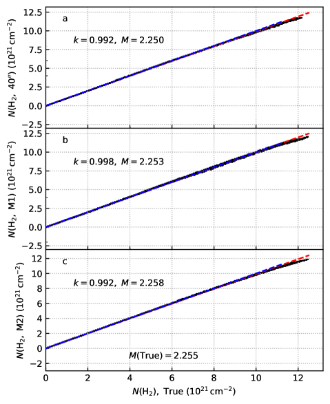
Figure 25: Correlations of column density estimates for the externally heated, lower column density model. The x-axis is the true column density of the model cloud at the resolution of 40$\arcsec$ (frame a) or 18$\arcsec$ (frames b and c). On the y-axes are the results from direct MBB fits at 40$\arcsec$ resolution (frame a) and from methods A and B at 18$\arcsec$ resolution (frames b and c, respectively). The dashed blue lines show the one-to-one relations and the dashed red lines the least squares fits. The slopes $k$ of the least squares lines as well as the estimated cloud masses (in solar masses) are given in the frames. The true mass of the cloud is quoted in frame c.

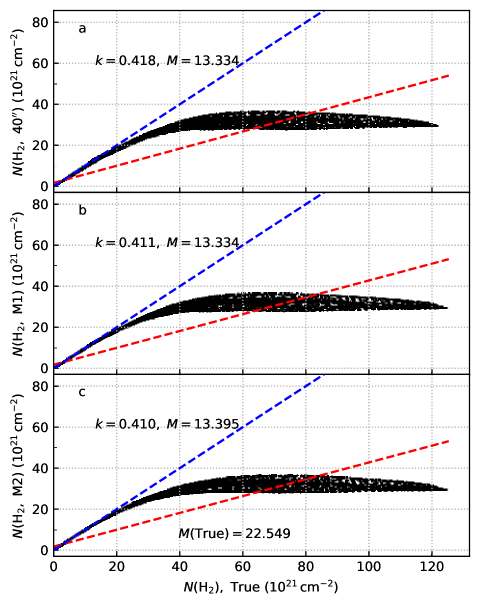
Figure 26: Same as Fig.25 but for the higher column density model.

Figure 25 shows results for the lower column density model with only external illumination and without observational noise. The figure also includes column density estimates calculated from data convolved to 40$\arcsec$. One pixel of the radiative transfer model corresponded to 1$\arcsec$, which means that structures are well resolved. All estimates are in good agreement with the true column density values.

The situation is different for the high column density model (Fig. 26). The column densities are severely underestimated above $N({\rm H}_{2})=2\times 10^{22}$ cm^-2. The estimates are actually decreasing towards the highest column densities and the maximum error is close a factor of 4. The methods A and B give practically identical results. Figure 27 shows the method B fit in the form of maps. Because of LOS temperature variations, the observed spectrum is much wider than the best-fit MBB function, and the maximum residuals exceed 10% of the measured surface brightness.

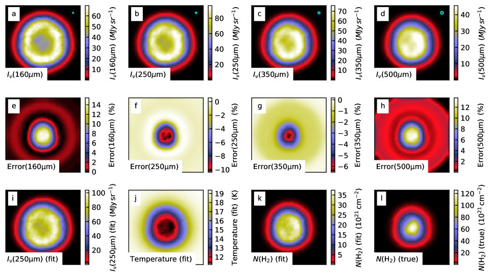
Figure 27: Fit of the simulated observations of the high-column-density model without observational noise. The first row shows the synthetic surface brightness maps with the beam size indicated in the upper right corner. The second row shows the relative fit residuals. Frames i-j show the fitted model parameters, the 250 $\mu$m surface brightness and the colour temperature. Frames k-l compare the final column density map at 10$\arcsec$ resolution to the true column density.

Figures 28 and 29 show the results for the high-column-density model after the addition of internal sources. At the highest column densities method B now results in marginally higher column density estimates than method A. Although the presence of internal heating has significantly reduced the bias, both methods underestimate the true column density by up to 25%. The point sources are barely resolved. If the resolution of the observations is degraded by a factor of three, the results of the methods A and B are identical.

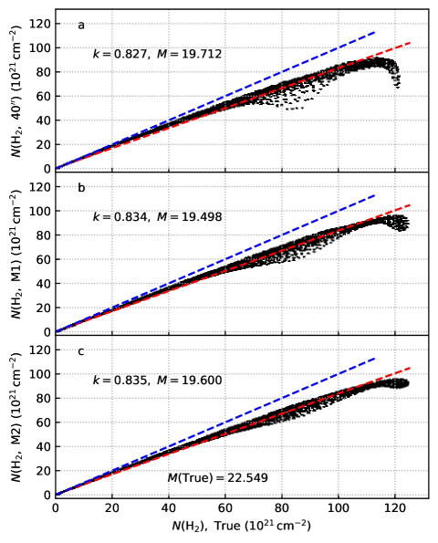
Figure 28: As Fig.26 but with added internal heating sources.

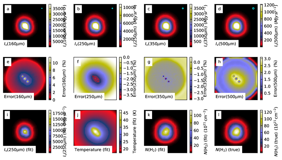
Figure 29: As Fig. 27 but with added internal heating sources.

We repeated the tests after adding to the synthetic observations Gaussian noise equal to the error estimates of the observations. Figures 30-31 show the results for lower resolution observations where the original model pixel corresponds to 0.3$\arcsec$. For the lower column density model the differences are not significant, although the scatter of the $N({\rm H}_{2})$ estimates is marginally smaller for Method B (Fig. 30). The results at higher column densities (Fig. 31) are qualitatively similar to those without noise (Fig. 26). Method B again exhibits slightly smaller dispersion, especially at low-column-densities. This is due to the global nature of the solution with some additional effect from the regularisation. Apart from this, the results of the two methods are in practice identical.

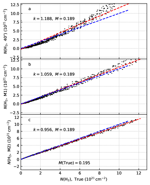
Figure 30: As Fig. 25 but with a factor of three lower spatial resolution and with added observational noise. In each frame the lower right corner shows the zoom-in to a column density range from zero to 10²¹ cm^-2. The rms dispersion relative to the linear least-squares fit is indicated in each frame.

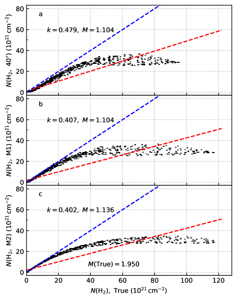
Figure 31: As Fig. 30 but for the models with higher column density. Compared to Fig. 28 the spatial resolution is lower by a factor of three and the data include added observational noise.

Appendix B Fit of the ($I$, $Q$, $U$) data of Planck and POL-2

Because of the apparent dissimilarity of the Planck and JCMT POL-2 polarisation maps, we tested their consistency by making a model that consisted of ($I$, $Q$, $U$) maps. These model maps were optimised through comparison with the Planck and POL-2 observations, both at their original resolutions. In the case of POL-2, the filtering of low spatial frequencies was simulated by subtracting a map obtained by convolving the observations with a Gaussian beam with $\theta=300\arcsec$. In the main text, the filtering was assumed to be stronger with $\theta=200\arcsec$ and this would make it even easier to reconcile any differences between the instruments. The model ($I$, $Q$, $U$) maps had a pixel size of 10$\arcsec$. The model optimisation took into account the error estimates (see Sect. 2) and the degree to which the model was oversampled compared to the observations.

The results are shown in Fig. 32. The obtained ($I$, $Q$, $U$) images fit well both the Planck and POL-2 data. In spite of the uncertainties (for example, the true nature of POL-2 filtering), the exercise shows that there is no discrepancy between the data sets but also that the spatial filtering plays a major role in the magnetic field morphology seen in the POL-2 data.

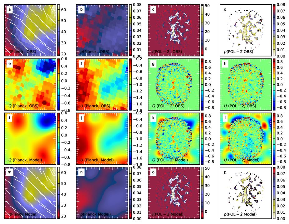
Figure 32: Results for the combined ($I$, $Q$, $U$) fir to Planck and POL-2 data. Frames a-d show the observed Planck and POL-2 surface brightness data and polarisation fraction maps. Frames a and c also show the polarisation vectors based on observations. The second row shows the observed Planck and POL-2 maps of $Q$ and $U$. The third and fourth rows show the ($I$, $Q$, $U$) maps of the fitted model. In frames c and o polarisation vectors are drawn only in regions with $I(850\mu{\rm m})>5$ MJy sr^-1.

Appendix C Effect of noise on the relations between $p$, $N$, and $S$

Noise affects the estimated values of both polarisation angles and polarisation fraction (e.g. Montier et al. 2015a; Fissel et al. 2016). In the following we use simulations to estimate the effect of noise on the observed relations between polarisation fraction, column density, and polarisation angle dispersion function. In the case of polarisation fraction, we always refer to $p_{\rm mas}$ estimates that are already corrected for bias, as described in Sect. 3.2. The correction is reliable at $p_{\rm mas}/\sigma_{p,\rm mas}>2$ but values at lower SNR can be expected to be biased (Montier et al. 2015b). However, even biased data contain some information, which can be used when data are compared to simulated observations.

Figure 13 showed a negative correlation between the $p_{\rm mas}$ and $S$ values estimated from Planck data. Such a trend could result from noise if that causes significant bias in the polarisation fraction estimates. For comparison with Fig. 13, we made a simulation using the average error estimates of the Planck data (including the covariances) but assuming constant values for both polarisation angles and polarisation fractions. The results are shown in Fig. 33. At full Planck resolution, noise increases the typical $S$ values that, nevertheless, are only a fraction of the values in Fig. 13. The polarisation fraction estimates show some dispersion but the values are unbiased. As a result, the $p_{\rm mas}(S)$ relation shows no significant correlations, unlike in the actual observations shown in Fig. 13c.

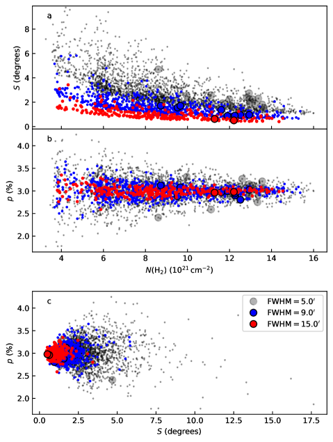
Figure 33: Polarisation angle dispersion function $S$ and polarisation fraction $p_{\rm mas}$ based on simulated Planck data that assume a constant polarisation angle and a constant polarisation fraction of 3%. Frames a and b show these as a function of dust optical depth and frame c shows their mutual correlation. The colours correspond to the data resolution, as indicated in frame c. The points inside the area mapped with POL-2 are plotted with large symbols. The data are sampled at steps of FWHM/2 and $S$ is calculated for lag $\delta=$FWHM/2.

We examined the $p_{\rm mas}$ vs. $N$ relation of POL-2 data as a function of the resolution. Lower resolution may increase geometrical depolarisation but, more importantly, increases the SNR and thus reduces the noise bias. In Fig. 34, we plot $p_{\rm mas}$ as a function of column density at the resolutions of 20$\arcsec$, 40$\arcsec$, and 80$\arcsec$. Only data with $N({\rm H}_{2})>7.5\times 10^{21}$ cm^-2 are used for linear fits. As the resolution is reduced, the slope decreases. Above $N({\rm H}_{2})\sim 20\times 10^{21}$ cm^-2 the polarisation fraction is nevertheless 1-2%, irrespective of the resolution.

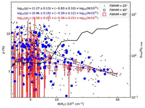
Figure 34: Polarisation fraction $p_{\rm mas}$ as a function of column density, based on POL-2 data at 20$\arcsec$, 40$\arcsec$, and 80$\arcsec$ resolution. The data are sampled at half-beam steps. The dashed lines correspond to least squares fits data $N({\rm H}_{2})>7.5\times 10^{21}$ ${\rm cm}^{-2}$. The error bars are shown only for the FWHM=$80\arcsec$ data points. The solid black line and the right-hand y-axis show the median SNR for polarisation fraction, $p_{\rm mas}/\sigma_{p,\/\rm mas}$, at $40\arcsec$ resolution.

For comparison with Fig. 34, Fig. 35 shows simulations of the $p_{\rm mas}$ vs. $N$ relation in the presence of noise. The simulations assumed that the true polarisation fraction is constant 1.5% and the observed $p$ depends on the column density only because of the noise bias. The observed intensity was assumed to be directly proportional to the column density. The SNR of the total intensity at $N({\rm H}_{2})=10^{22}$ ${\rm cm}^{-2}$ is either 40 or 100. In the observations, the SNR is not constant for a given column density and the values at $N({\rm H}_{2})=10^{22}$ ${\rm cm}^{-2}$ range from SNR$\sim$10 to SNR$\sim$70 with a mean value of $\sim$33. Thus the SNR=100 simulation could define a lower envelope for $p_{\rm mas}$, the observed values being higher because of the noise bias. Above $N({\rm H}_{2})=2\times 10^{22}\,{\rm cm}^{-2}$ the average SNR is SNR$\sim$100 or higher (see Fig.34).

In Fig. 35, when the data are convolved to a lower resolution, the SNR increases and the $p_{\rm mas}$ values decrease. Eventually the high-$N({\rm H}_{2})$ values become independent of the convolution while the polarisation fractions still decrease at lower $N({\rm H}_{2})$. At 40$\arcsec$ resolution $p$ values become reliable only at $N({\rm H}_{2})>10^{22}$ ${\rm cm}^{-2}$, where the average SNR of observations is above 100 for the total intensity.

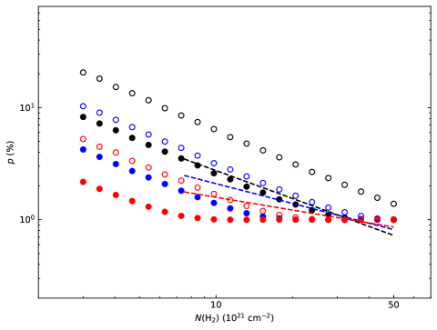
Figure 35: Simulations of the $p_{\rm mas}$ vs. $N$ relations in POL-2 observations. The calculations assumed a regular field (no geometrical depolarisation), an intrinsic polarisation fraction of $p=1\%$, and intensities proportional to the column density. The initial SNR of the total intensity at $N({\rm H}_{2})=10^{22}$ cm^-2 at the full FWHM=15$\arcsec$ resolution is either 40 (open circles) or 200 (solid circles). The black, blue, and red colours correspond to the convolution to a resolution of 20$\arcsec$, 40$\arcsec$, and 80$\arcsec$, respectively. For comparison, the dashed lines show the least squares fits from Fig. 34.

In Fig. 14 we concluded that the anticorrelation would be true, based on the SNR of the selected data (Fig. 9) and the formal errors of the fitted least squares lines. We examined this more directly using the observed ($I$, $Q$, $U$) data and their error estimates. We rescaled ($Q$, $U$) so that they corresponded to a flat relation $p=1.5$%. We constructed synthetic data sets where noise was added according to the POL-2 error maps and the $p_{\rm mas}(N)$ relation was fitted with a weighted least squares line. The simulation was repeated 2000 times for a number of column density thresholds. Figure 36 indicates that there is over 99% probability that the observed slope is steeper than what is expected based on the constant-$p$ assumption. The slopes become uncertain for thresholds $N({\rm H}_{2})>3\times 10^{22}$ cm^-2 because the fitted dynamical range and the number of data points decrease. The significance also decreases below $N({\rm H}_{2})\sim 10^{22}$ cm^-2 when data become dominated by noise. In between, the observed slope is much steeper than in the simulations. Note that it is not necessary for the $p_{\rm mas}$ estimates be completely unbiased, because the bias should be the same both for the real and the simulated observations. The significance of the result could be decreased only if the uncertainties of $Q$ and $U$ were underestimated, for example because of artefacts caused by the spatial filtering or the mapping procedure.

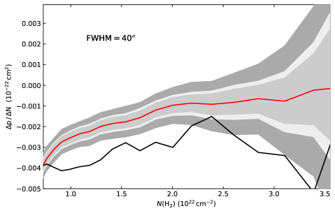
Figure 36: Simulation of $p_{\rm mas}$ vs. $N$ relation for POL-2 data. The figure shows the slopes of the fitted least squares lines as a function of the column density threshold used to select data. The black line shows the fits to the original observations. The red curve shows the median slope for simulations that assume an intrinsically constant polarisation fraction of $p=1.5\%$ and the shaded areas correspond to [1%,99%], [10%,90%], and [16%,84%] confidence intervals.

In Fig. 34 the slope was observed to change systematically as a function of the data resolution. We carried out separate calculation to examine the potential contribution of geometrical depolarisation to this relation. Using data with $N({\rm H}_{2})>10^{22}$ cm^-2, we plot in Fig. 37 the observed average polarisation fraction $\langle p_{\rm mas}\rangle$ as a function of the spatial resolution. This is compared to two simulations that start with the 20$\arcsec$ resolution observations. First simulation assumes that these observations represent the true (noiseless) polarisation data. We produce synthetic observations by adding noise according to the POL-2 error estimates and plot again $\langle p_{\rm mas}\rangle$ as a function of the resolution. This is thus identical to the actual observations, except for the added noise. In the second simulation ($Q$, $U$) are first rotated so that polarisation angle is the same in each pixel. This means that the resolution only affects the noise level but there is no geometrical depolarisation.

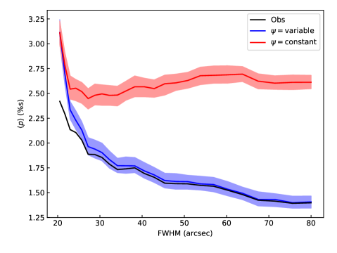
Figure 37: Simulation of $\langle p\rangle$ for POL-2 data with $N({\rm H}_{2})>10^{22}$ cm^-2 as a function of the resolution. The black line shows the relation for the original observations. The blue line corresponds to a case where ($Q$, $U$) observed at 20$\arcsec$ resolution are taken as a model of the true signal, before adding observational noise and convolving to a lower resolution. The red curve shows the result for data with identical $p$ and $I$ but with a globally constant polarisation angle. The shaded regions show the [10%, 90%] ranges for the random realisations.

Figure 37 shows that without geometrical depolarisation the $\langle p\rangle$ does not decrease beyond FWHM$\sim 30\arcsec$, in agreement with SNR plotted in Fig. 9. On the contrary, there is minor increase towards lower resolutions. This is probably caused by the negative correlation between $p$ and $N({\rm H}_{2})$, which means that, for a given column density threshold, the average SNR of polarised intensity decreases as a function of the beam size. The simulation that included polarisation angle variations naturally converges towards the observed curve. The results indicate that between the 20$\arcsec$ and 80$\arcsec$ resolutions, more than half of the drop is caused by geometrical depolarisation and a smaller part by the reduced noise bias.

Appendix D Alternative RT models for polarised emission

In this section we show two variants of the polarisation models presented in Sect. 5.2.

Figure  38 shows results for constant grain alignment. It is the same as Fig. 18 except that the transition from the uniform large-scale field to the filament field (as defined by the magnetic field toy model) takes place at a higher volume density threshold that is $n({\rm H}_{2})=10^{4}$ cm^-3 instead of $n({\rm H}_{2})=3\times 10^{3}$ cm^-3. This leads to decrease in the polarisation fractions, especially in the northern clump.

Figure 39 corresponds to calculations with RAT grain alignment and grain sizes that are a factor of two larger than in the original dust model. The figure differs from Fig. 39 in that the POS magnetic field orientations are taken from POL-2 observations instead of the toy model of Sect. 5.2. The polarisation fractions show a small decrease. Part of the changes may be caused by noise in the input polarisation angles, which here contributes to the geometrical depolarisation (that is, angle dispersion within the beam).

Figure 38: Predictions of polarised emission for a RT model with constant grain alignment, using the toy magnetic field model. The figure is the same as in Fig. 18 except that the transition from the large-scale field to different field orientations in the filament takes place at a higher threshold of $n({\rm H}_{2})=10^{4}$ cm^-3. The polarisation vectors are shown on the column density map in frame a and the $p$ vs. $N({\rm H}_{2})$ relation is plotted in frame b at Planck resolution. The lower frames are the corresponding plots for synthetic POL-2 observations.

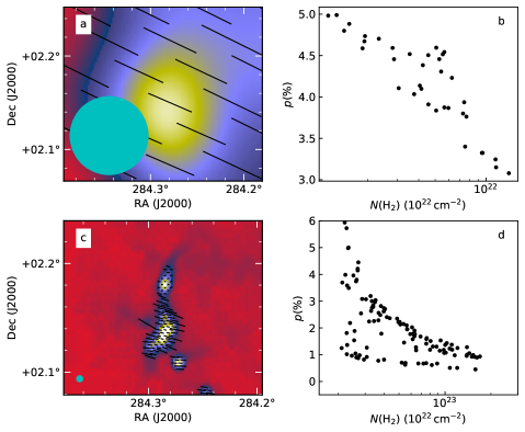
Figure 39: Model predictions for polarisation according to RAT grain alignment, assuming larger grain sizes. The figure is the same as Fig. 20 but the field orientation in the filament with $n({\rm H}_{2})>3\times 10^{3}$ cm^-3 is taken directly from POL-2 observations at 20$\arcsec$ resolution.