Charged lepton flavor violation and electric dipole moments in the inert Zee model

Abstract

The inert Zee model is an extension of the Zee model for neutrino masses to allow for a solution to the dark matter problem that involves two vector-like fields, a doublet and a singlet of $SU(2)_{L}$, and two scalars, also a doublet and a singlet of $SU(2)_{L}$, all of them being odd under an exact $Z_{2}$ symmetry. The introduction of the $Z_{2}$ guarantees one-loop neutrino masses, forbids tree-level Higgs-mediated flavor changing neutral currents and ensures the stability of the dark matter candidate. Due to the natural breaking of lepton numbers in the inert Zee model and encouraged by the ambitious experimental program designed to look for charged lepton flavor violation signals and the electron electric dipole moment, we study the phenomenology of the processes leading to these kind of signals, and establish which are the most promising experimental perspectives on that matter.

I Introduction

Neutrino oscillations Fukuda:1998mi ; Ahmad:2002jz provide a clear evidence for lepton flavor violation (LFV) in the neutral sector, pointing out to physics beyond the Standard Model (SM). However, no evidence of lepton flavor violating processes in the charged sector has been found despite the great experimental effort on searching for that violation Lindner:2016bgg ; Calibbi:2017uvl . Indeed, the experimental searches not only have reached a great sensitivity but will also be improved in the near future by, in some cases, several orders of magnitude. For instance, the MEG collaboration has reported an upper limit on the decay branching ratio for the rare decay $\mu\to e\gamma$ around $6\times 10^{-13}$ Adam:2013mnn , which will be improved soon by a factor of 10 Baldini:2013ke . Concerning the three-body decay $\mu\rightarrow 3e$, the negative searches for rare decays in the SINDRUM experiment lead to an upper limit for the branching ratio of around $10^{-12}$ Bellgardt:1987du , whereas the Mu3e experiment collaboration expects to reach the ultimate sensitivity to test such a decay in $10^{16}$ muon decays Blondel:2013ia . In addition, the neutrinoless $\mu$-$e$ conversion in muonic atoms is also a promising way to search for charged LFV (CLFV) signals due to the significant increase of sensitivity (up to six orders of magnitude) expected for this class of experiments Carey:2008zz ; Glenzinski:2010zz ; Abrams:2012er ; Aoki:2010zz ; Natori:2014yba ; Cui:2009zz ; Kuno:2013mha ; Barlow:2011zza . Last but not least, the future plans regarding electron electric dipole moment (eEDM) Kara:2012ay ; Kawall:2011zz are also in quest for New Physics signals since the expected sensitivity for these facilities will improve by two orders of magnitude the current bound $|d_{e}|<8.7\times 10^{-29}e\,\cdot\,$cm Baron:2013eja . This ambitious experimental program, in turn, calls for a deep phenomenological analysis of the CLFV and EDM signals in models featuring new charged lepton interactions such as those undertaking neutrino masses.

On the other hand, despite the abundant and compelling evidence for the massiveness of neutrinos Patrignani:2016xqp ; deSalas:2017kay , the underlying mechanism behind it remains unknown, which is not a bizarre occurrence since the particle theory responsible for the dark matter (DM) of the Universe also resists to be experimentally elucidated. Hence, it would desirable that both phenomena may have a common origin with a New Physics laying at the electroweak scale, as happens in the radiative neutrino mass models involving a dark matter candidate at or below the TeV scale Brdar:2013iea ; Restrepo:2013aga ; Chen:2014ska ; Ahriche:2016ixu ; Simoes:2017kqb ; Yao:2017vtm ; Yao:2018ekp . Thus, the resulting model not only would constitute a way out to two of the open questions in the SM but also would have the additional bonus that the new particles may induce potentially large rates for the CLFV and EDM processes, give rise to novel observable phemomena at the LHC, and lead to signals in direct and indirect DM experiments.

In this work we consider the inert Zee model (IZM) -a dark matter realization of the Zee model for neutrino masses Zee:1980ai ; Wolfenstein:1980sy ; Petcov:1982en where the above features are present-, with the aim of pursuing a dedicated analysis of LFV processes and EDM signals. As in the Zee model, neutrino masses are generated at one loop, while DM is addressed as in the inert doublet model Barbieri:2006dq ; LopezHonorez:2006gr ; Honorez:2010re ; LopezHonorez:2010tb ; Goudelis:2013uca ; Garcia-Cely:2013zga ; Arhrib:2013ela since both models share a $Z_{2}$-odd scalar $SU(2)_{L}$ doublet. In addition, due to the new interactions, the IZM has a richer phenomenology than the minimal scotogenic model Ma:2006km . Once we will have determined the viable parameter space consistent with dark matter, neutrino oscillation observables, lepton-flavor violating processes and electroweak precision tests, we will establish the most relevant experimental perspectives regarding LFV searches. Furthermore, since the Yukawa couplings that reproduce the neutrino oscillation data are complex, which in turn constitute new sources of CP violation, we will look into the regions in the parameter space where the prospects for the eEDM are within the future experimental sensitivity Kara:2012ay ; Kawall:2011zz ; Baron:2013eja . Lastly, we will also study the possible connection, via lepton Yukawa interactions, that may exist between DM and the anomalous magnetic dipole moment of the muon Bai:2014osa ; Kile:2014jea ; Chen:2015jkt ; Kowalska:2017iqv ; Calibbi:2018rzv .

The paper is organized as follows: in Sec. II we present the generalities of the model, including neutrino masses and dark matter. In Sec. III we study the LFV processes, the EDM and the magnetic dipole moment (MDM) of charged leptons. Their phenomenology is presented in Sec. IV. Finally, we conclude in Sec. V.

II The Model

The new particle content of the model Restrepo:2013aga ; Longas:2015sxk consists of two vectorlike fermions, a $SU(2)_{L}$-singlet $\epsilon$ and a $SU(2)_{L}$-doublet $\Psi=(N,E)^{\text{T}}$, and two scalar multiplets, a $SU(2)_{L}$-singlet $S^{-}$ and a $SU(2)_{L}$-doublet $H_{2}=(H_{2}^{+},H_{2}^{0})^{\text{T}}$. All of them are odd under the $Z_{2}$ symmetry, which in turn allows us to avoid Higgs-mediated flavor changing neutral currents at tree-level, forbid tree-level contributions to the neutrino masses and render the lightest $Z_{2}$-odd particle stable Longas:2015sxk . It follows that the most general $Z_{2}$-invariant Lagrangian of the model can be written as

$$\mathcal{L}_{\text{IZM}}=\mathcal{L}_{\text{SM}}+\mathcal{L}_{F}+\mathcal{L}_{S}+\mathcal{L}_{1}+\mathcal{L}_{2},$$ (1)

where $\mathcal{L}_{\text{SM}}$ is the SM Lagrangian which includes the Higgs potential $\mathcal{V}_{H_{1}}=\mu_{1}^{2}H_{1}^{\dagger}H_{1}+\lambda_{1}/2(H_{1}^{\dagger}H_{1})^{2}$, with $H_{1}=(0,H_{1}^{0})^{\text{T}}$, $H_{1}^{0}=(h+v)/\sqrt{2}$, $h$ being the Higgs boson and $v=246$ GeV. $\mathcal{L}_{F}$ and $\mathcal{L}_{S}$ comprise, respectively, the kinetic and mass terms for the new fermions, and the kinetic, mass and self-interacting terms of the new scalars,

$$\mathcal{L}_{F} =\bar{\Psi}(i\cancel{D}-m_{\Psi})\Psi+\bar{\epsilon}(i\cancel{D}-m_{\epsilon})\epsilon,$$ (2)

$$\mathcal{L}_{S} =(D_{\mu}H_{2})^{\dagger}(D^{\mu}H_{2})-\mu_{2}^{2}H_{2}^{\dagger}H_{2}-\frac{\lambda_{2}}{2}(H_{2}^{\dagger}H_{2})^{2}+(D_{\mu}S)^{\dagger}(D^{\mu}S)-\mu_{S}^{2}S^{\dagger}S-\lambda_{S}(S^{\dagger}S)^{2}.$$ (3)

The interaction terms between the scalars are included in $\mathcal{L}_{1}$,

$$-\mathcal{L}_{1} =\lambda_{3}(H_{1}^{\dagger}H_{1})(H_{2}^{\dagger}H_{2})+\lambda_{4}(H_{1}^{\dagger}H_{2})(H_{2}^{\dagger}H_{1})+\frac{\lambda_{5}}{2}\left[(H_{1}^{\dagger}H_{2})^{2}+{\rm h.c.}\right]$$

$$+\lambda_{6}(S^{\dagger}S)(H_{1}^{\dagger}H_{1})+\lambda_{7}(S^{\dagger}S)(H_{2}^{\dagger}H_{2})+\mu\epsilon_{ab}\left[H_{1}^{a}H_{2}^{b}S+{\rm h.c.}\right],$$ (4)

where $\epsilon_{ab}$ is the $SU(2)_{L}$ antisymmetric tensor with $\epsilon_{12}=1$, $H_{2}=(H_{2}^{+},H_{2}^{0})^{\text{T}}$ with $H_{2}^{0}=(H^{0}+iA^{0})/\sqrt{2}$, and the scalar couplings $\lambda_{5}$ and $\mu$ are assumed real. It is worth mentioning that $H_{2}^{0}$ does not develop a vacuum expectation value in order to ensure the conservation of the $Z_{2}$ symmetry. Note that the scalar potential is rather similar to one of the singlet-doublet scalar DM model Kadastik:2009dj ; Kadastik:2009cu ; Kakizaki:2016dza ; Liu:2017gfg or two Higgs doublet models plus a scalar singlet, see e.g. Refs. Chen:2013jvg ; Muhlleitner:2016mzt , with the main difference that our $SU(2)_{L}$-singlet scalar is electrically charged (which in turn implies that $S$ has also a null vacuum expectation value and that the charged scalars get mixed instead of neutral ones). Finally, $\mathcal{L}_{2}$ includes the new Yukawa interaction terms:

$$-\mathcal{L}_{2} =\eta_{i}\bar{L}_{i}H_{2}\epsilon+\rho_{i}\bar{\Psi}H_{2}e_{Ri}+y\bar{\Psi}H_{1}\epsilon+f^{*}_{i}\overline{L^{c}_{i}}\Psi S^{+}+{\rm h.c},$$ (5)

where $L_{i}$ and $e_{Ri}$ ($i=1,2,3)$ are the SM leptons, doublets and singlets of $SU(2)_{L}$, respectively. $\eta_{i}$, $\rho_{i}$ and $f_{i}$ are Yukawa couplings controlling the new lepton interactions, while $y$ leads to the mixing among the $Z_{2}$-odd charged fermions. Note that only $\eta_{i}$ and $f_{i}$ involve neutrino interactions, so they are the ones participating in the neutrino mass generation.

After electroweak symmetry breaking, the $Z_{2}$-odd scalar spectrum consists of a CP-even state $H^{0}$ and a CP-odd state $A^{0}$, and two charged states $\kappa_{1,2}$. Their masses are given by

$$m^{2}_{H^{0},A^{0}} =\mu_{2}^{2}+\frac{1}{2}\left(\lambda_{3}+\lambda_{4}\pm\lambda_{5}\right)v^{2},$$ (6)

$$m_{\kappa_{1},\kappa_{2}}^{2} =\frac{1}{2}\left\{m_{H^{\pm}}^{2}+m_{S^{\pm}}^{2}\mp[(m_{H^{\pm}}^{2}-m_{S^{\pm}}^{2})^{2}+2\mu^{2}v^{2}]^{1/2}\right\},$$ (7)

where $m_{H^{\pm}}^{2}=\mu_{2}^{2}+\frac{1}{2}\lambda_{3}v^{2}$ and $m_{S^{\pm}}^{2}=\mu_{S}^{2}+\frac{1}{2}\lambda_{6}v^{2}$. The scalar mixing angle $\delta$ is defined through $\sin{2\delta}=(\sqrt{2}\mu v)/(m_{\kappa_{2}}^{2}-m_{\kappa_{1}}^{2})$. On the other hand, the $Z_{2}$-odd fermion spectrum involves two charged fermions $\chi_{1,2}$ with

$$m_{\chi_{1,2}} =\frac{1}{2}\left\{m_{\Psi}+m_{\epsilon}\mp[(m_{\Psi}-m_{\epsilon})^{2}+2y^{2}v^{2}]^{1/2}\right\},$$ (8)

and a mixing angle given by $\sin{2\alpha}=(\sqrt{2}yv)/(m_{\chi_{2}}-m_{\chi_{1}})$, along with the neutral Dirac fermion $N$, with a mass $m_{N}=m_{\Psi}$ fulfilling $m_{\chi_{1}}\leq m_{N}\leq m_{\chi_{2}}$.

With respect to DM in the IZM, $H^{0}$ is the DM candidate as long as it remains as the lightest $Z_{2}$-odd particle in the spectrum. Hence, we expect the DM phenomenology to be similar to the one in the inert doublet model (IDM) in scenarios where the particles not belonging to the IDM ($\kappa_{1,2}$, $\chi_{1,2}$ and $N$) do not participate in the DM annihilation processes Longas:2015sxk . Accordingly, the viable DM mass range for this scenario (the same of the one in the IDM) is divided into two regimes Barbieri:2006dq ; LopezHonorez:2006gr ; Honorez:2010re ; LopezHonorez:2010tb ; Goudelis:2013uca ; Garcia-Cely:2013zga ; Arhrib:2013ela : the low mass regime, $m_{H^{0}}\simeq m_{h}/2$, and the high mass regime, $m_{H^{0}}\gtrsim 500$ GeV. Since in the latter regime the CLFV processes are quite suppressed (the corresponding rates scale as $m_{\chi_{\omega}}^{-4}$ or $m_{\kappa_{\beta}}^{-4}$), in our numerical analysis we will only consider the low mass regime.

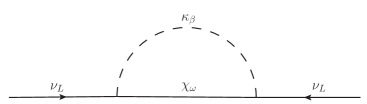
Figure 1: One-loop diagram leading to neutrino Majorana masses.

In this model the neutrino masses are generated at one-loop thanks to the scalar and fermion mixings and to the Yukawa interactions mediated by $\eta_{i}$ and $f_{i}$. From Fig. 1, the neutrino mass matrix in the mass eigenstates is given by

$$[M_{\nu}]_{ij} =\zeta[\eta_{i}f_{j}+\eta_{j}f_{i}],$$ (9)

where $\zeta=(\sin 2\alpha\sin 2\delta)/(64\pi^{2})\sum_{n}c_{n}m_{\chi_{n}}I(m_{\kappa_{1}}^{2},m_{\kappa_{2}}^{2},m_{\chi_{n}}^{2})$, $c_{1}=-1$, $c_{2}=+1$ and $I(a,b,c)=b\ln(b/c)/(b-c)-a\ln(a/c)/(a-c)$. Note that for a vanishing scalar or fermion mixing the neutrino masses are zero and that, due to the flavor structure of $M_{\nu}$, the lightest neutrino is massless. This, the masslessness of the lightest neutrino, entails several phenomenological consequences: $i)$ there is only single Majorana CP phase since the second phase can be absorbed by a redefinition of the massless neutrino field; $ii)$ the two remaining neutrino masses are entirely set by the solar and atmospheric mass scales: for normal hierarchy (NH) $m_{1}=0$, $m_{2}=\sqrt{\Delta m_{\text{sol}}^{2}}$ and $m_{3}=\sqrt{\Delta m_{\text{atm}}^{2}}$, while for inverted hierarchy (IH) $m_{1}=\sqrt{\Delta m_{\text{atm}}^{2}}$, $m_{2}=\sqrt{\Delta m_{\text{sol}}^{2}+m_{1}^{2}}\approx\sqrt{\Delta m_{\text{atm}}^{2}}$ and $m_{3}=0$; $iii)$ the amplitude for neutrinoless double beta decay Rodejohann:2011vc presents a lower bound, which for the case of IH lies within the sensitivity of future facilities dedicated for that goal Reig:2018ztc .

In Ref. Longas:2015sxk it was shown that, using Eq. (9) and the diagonalization condition $U^{\text{T}}M_{\nu}U={\rm diag}(m_{1},m_{2},m_{3})$ with $U=VP$ and $P=\mbox{diag}(1,e^{i\phi/2},1)$ Agashe:2014kda , it is possible to express five of the six Yukawa couplings $\eta_{i}$ and $f_{i}$ in terms of the neutrino low energy observables. Consequently, the most general Yukawa couplings that are compatible with the neutrino oscillation data are given by

$$\eta_{i}=|\eta_{1}|\frac{A_{i}}{\beta_{11}},\hskip 28.45274ptf_{i}=\frac{1}{2\zeta}\frac{\beta_{ii}}{\eta_{i}},$$ (10)

where

$$\beta_{ij} =e^{i\phi}m_{2}V_{i2}^{*}V_{j2}^{*}+m_{3}V_{i3}^{*}V_{j3}^{*},$$

$$A_{j} =\pm\sqrt{-e^{i\phi}m_{2}m_{3}(V_{12}^{*}V_{j3}^{*}-V_{13}^{*}V_{j2}^{*})^{2}e^{i2\text{Arg}(\eta_{1})}}+\beta_{1j}e^{i\text{Arg}(\eta_{1})},\,\,\,\mbox{for NH},$$ (11)

$$\beta_{ij} =m_{1}V_{i1}^{*}V_{j1}^{*}+e^{i\phi}m_{2}V_{i2}^{*}V_{j2}^{*},$$

$$A_{j} =\pm\sqrt{-e^{i\phi}m_{1}m_{2}(V_{11}^{*}V_{j2}^{*}-V_{12}^{*}V_{j1}^{*})^{2}e^{i2\text{Arg}(\eta_{1})}}+\beta_{1j}e^{i\text{Arg}(\eta_{1})},\,\,\,\mbox{for IH}.$$ (12)

In this way, it is always possible to correctly reproduce the neutrino oscillation parameters in the present model.

III Charged lepton processes

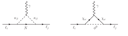
Figure 2: One-loop diagrams leading to eEDM, anomalous muon MDM, and $\ell_{i}\rightarrow\ell_{j}\gamma$ decays when $i=j=1$, $i=j=2$ and $i\neq j$, respectively. Here $\phi^{0}$ denotes the two $Z_{2}$-odd neutral scalars $A^{0}$ and $H^{0}$.

Once lepton flavor violation is allowed via neutrino Majorana masses, LFV processes involving charged leptons such as $\ell_{i}\rightarrow\ell_{j}\gamma$, $\ell_{i}\rightarrow 3\ell_{j}$ and $\mu-e$ conversion in nuclei are unavoidable. In the IZM model such processes are generated at one-loop level involving the $\eta_{i}$, $f_{i}$ and $\rho_{i}$ Yukawa interactions (see Eq. (5)), which in turn implies that they are mediated by, both charged and neutral, $Z_{2}$-odd fermions and scalars. It is worth mentioning that $\rho_{i}$ may enhance the rates for the CLFV processes and EDMs since it is not subject to the neutrino oscillation constraints (only $\eta_{i}$ and $f_{i}$ enter in the neutrino mass generation).

The triangle diagrams leading to $\ell_{i}\rightarrow\ell_{j}\gamma$ processes are displayed in Fig. 2. The corresponding branching ratios (neglecting lepton masses at final states) are given by

$$\mathcal{B}\left(\ell_{i}\rightarrow\ell_{j}\gamma\right)=\frac{3\alpha_{em}}{64\pi m_{\mu}^{2}G_{F}^{2}}\left(\left|\Sigma_{L}\right|^{2}+\left|\Sigma_{R}\right|^{2}\right)\mathcal{B}\left(\ell_{i}\rightarrow\ell_{j}\nu_{i}\bar{\nu_{j}}\right),$$ (13)

where $\alpha_{em}$ is the electromagnetic fine structure constant, $G_{F}$ is the Fermi constant and $\Sigma_{L}$, $\Sigma_{R}$ are given by

$$\Sigma_{L}= -\eta_{i}^{*}\rho_{j}^{*}s_{\alpha}c_{\alpha}\left[m_{\chi_{1}}\mathcal{G}_{1}(m^{2}_{\chi_{1}},m_{A^{0}}^{2},m_{H^{0}}^{2})-m_{\chi_{2}}\mathcal{G}_{1}(m^{2}_{\chi_{2}},m_{A^{0}}^{2},m_{H^{0}}^{2})\right]$$

$$-m_{\ell_{i}}\rho_{i}^{*}\rho_{j}\left[s^{2}_{\alpha}\mathcal{F}_{1}(m^{2}_{\chi_{2}},m_{A^{0}}^{2},m_{H^{0}}^{2})+c^{2}_{\alpha}\mathcal{F}_{1}(m^{2}_{\chi_{1}},m_{A^{0}}^{2},m_{H^{0}}^{2})\right]$$

$$+m_{\ell_{i}}\rho_{i}^{*}\rho_{j}\left[c^{2}_{\delta}\mathcal{F}_{2}(m^{2}_{\kappa_{1}},m_{N}^{2})+s^{2}_{\delta}\mathcal{F}_{2}(m^{2}_{\kappa_{2}},m_{N}^{2})\right]\;,$$ (14)

$$\Sigma_{R}= -\rho_{i}\eta_{j}s_{\alpha}c_{\alpha}\left[m_{\chi_{1}}\mathcal{G}_{1}(m^{2}_{\chi_{1}},m_{A^{0}}^{2},m_{H^{0}}^{2})-m_{\chi_{2}}\mathcal{G}_{1}(m^{2}_{\chi_{2}},m_{A^{0}}^{2},m_{H^{0}}^{2})\right]$$

$$-m_{\ell_{i}}\eta_{i}^{*}\eta_{j}\left[c^{2}_{\alpha}\mathcal{F}_{1}(m^{2}_{\chi_{2}},m_{A^{0}}^{2},m_{H^{0}}^{2})+s^{2}_{\alpha}\mathcal{F}_{1}(m^{2}_{\chi_{1}},m_{A^{0}}^{2},m_{H^{0}}^{2})\right]$$

$$+m_{\ell_{i}}f_{i}^{*}f_{j}\left[s^{2}_{\delta}\mathcal{F}_{2}(m^{2}_{\kappa_{1}},m_{N}^{2})+c^{2}_{\delta}\mathcal{F}_{2}(m^{2}_{\kappa_{2}},m_{N}^{2})\right]\;.$$ (15)

The loop functions are reported in the Appendix. Note that, in contrast to neutrino masses, these branching ratios are not double suppressed by the mixing of $Z_{2}$-odd particles. This implies that, as is expected, the rare decays $\ell_{i}\rightarrow\ell_{j}\gamma$ do not depend on whether neutrino masses are zero or not. On the other hand, note that the IZM has an additional contribution (right diagram) to $\ell_{i}\rightarrow\ell_{j}\gamma$ with respect to the minimal scotogenic model Ma:2006km . Indeed, in that diagram precisely enter $\rho_{i}$, the Yukawa couplings that are not affected by neutrino oscillation constraints.

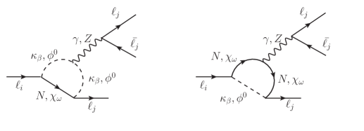
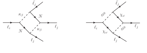
Figure 3: One-loop diagrams contributing to $\ell_{i}\rightarrow\ell_{j}\bar{\ell_{j}}\ell_{j}$ decays, where $\phi^{0}$ denotes the two $Z_{2}$-odd neutral scalars $A^{0}$ and $H^{0}$.

Concerning the $\ell_{i}\rightarrow\ell_{j}\bar{\ell_{j}}\ell_{j}$ there are two class of diagrams (see Fig. 3) leading to such processes: the $\gamma$- and $Z$- penguin diagrams (top panels) and the box diagrams (bottom panels). There is also a contribution from Higgs-penguin diagrams which, nevertheless, is suppressed for the first two charged leptons generations due to their small Yukawa couplings. The contribution of those processes involving tau leptons is not negligible but the corresponding limits are less restrictive. Therefore, the $\ell_{i}\rightarrow\ell_{j}\bar{\ell_{j}}\ell_{j}$ processes contain four kind of contributions: the photonic monopole, photonic dipole, $Z$-penguin and boxes. In contrast, the photonic dipole contribution is the only one present in $\ell_{i}\rightarrow\ell_{j}\gamma$ processes.

Finally, the $\mu-e$ conversion diagrams are obtained when the pair of lepton lines attached to the photon and $Z$ boson in the penguin diagrams (see top panels of Fig. 3) are replaced by a pair of light quark lines. There are no box diagrams since the $Z_{2}$-odd particles do not couple to quarks at tree level. Accordingly, the photonic non-dipole and dipole terms along the $Z-$penguin are the only terms that contribute to the $\mu-e$ conversion processes. Since the calculations of the $\ell_{i}\rightarrow\ell_{j}\bar{\ell_{j}}\ell_{j}$ and $\mu-e$ rates are quite involved, we implement the FlavorKit code Porod:2014xia to use the corresponding full expressions.

Since the parameters $\beta_{ij}$ and $A_{j}$ in Eqs. (11) and (12) are in general complex, it follows that the Yukawa couplings required for neutrino oscillation data constitute new sources of CP violation in the lepton sector. Thus the IZM brings with it new contributions to the EDM of charged leptons with the distinctive feature that the leading contribution arises at one-loop level (see right top diagram of Fig. 2 with $i=j=1$), in constrast with the one obtained in the minimal scotogenic model where it arises a two loops Abada:2018zra . Accordingly, large values for the eEDM may be expected. The analytical expression reads

$$d_{\ell_{i}}=\frac{e}{2^{6}\pi^{2}}s_{2\alpha}\operatorname{Im}(\rho_{i}\eta_{i})\left[m_{\chi_{2}}\mathcal{I}_{1}(m^{2}_{\chi_{2}},m_{H^{0}}^{2},m_{A^{0}}^{2})-m_{\chi_{1}}\mathcal{I}_{1}(m^{2}_{\chi_{1}},m_{H^{0}}^{2},m_{A^{0}}^{2})\right],$$ (16)

where the loop function is given in the Appendix. It is clear then that $d_{\ell_{i}}$ becomes suppressed for small fermion mixing angles. On the other hand, note that the left diagram of Fig. 2 does not contribute to the EDM because the neutral Dirac fermion, $N$, only has one single chiral coupling to either $\ell_{i}$ or $\ell^{c}_{i}$, i.e., such a diagram conserves CP.

Yukawa interactions also lead to contributions to anomalous magnetic dipole moments of the charged leptons. These contributions can be cast as

$$a_{\ell_{i}}^{\text{IZM}}=a_{\ell_{i}}^{\mathrm{F}}+a_{\ell_{i}}^{\mathrm{S}},$$ (17)

where

$$a_{\ell_{i}}^{\mathrm{F}} =\frac{m_{\ell_{i}}^{2}}{2^{5}\pi^{2}}\Big{[}\left(|\rho_{i}|^{2}c^{2}_{\alpha}+|\eta_{i}|^{2}s^{2}_{\alpha}\right)\mathcal{H}_{1}(m_{\chi_{1}}^{2},m_{H^{0}}^{2},m_{A^{0}}^{2})+\left(|\rho_{i}|^{2}s^{2}_{\alpha}+|\eta_{i}|^{2}c^{2}_{\alpha}\right)\mathcal{H}_{1}(m_{\chi_{2}}^{2},m_{H^{0}}^{2},m_{A^{0}}^{2})\Big{.}$$

$$\hskip 8.5359pt+\frac{1}{m_{\ell_{i}}}\Big{.}s_{2\alpha}\operatorname{Re}(\rho_{i}\eta_{i})[m_{\chi_{1}}\mathcal{I}_{1}(m_{\chi_{1}}^{2},m_{H^{0}}^{2},m_{A^{0}}^{2})-m_{\chi_{2}}\mathcal{I}_{1}(m_{\chi_{2}}^{2},m_{H^{0}}^{2},m_{A^{0}}^{2})]\Big{]},$$ (18)

$$a_{\ell_{i}}^{\mathrm{S}} =-\frac{m_{\ell_{i}}^{2}}{2^{4}\pi^{2}}\Big{[}[|\rho_{i}|^{2}c^{2}_{\delta}+|f_{i}|^{2}s^{2}_{\delta}]\mathcal{H}_{2}(m_{\kappa_{1}}^{2},m_{N}^{2})+[|\rho_{i}|^{2}s^{2}_{\delta}+|f_{i}|^{2}c^{2}_{\delta}]\mathcal{H}_{2}(m_{\kappa_{2}}^{2},m_{N}^{2})\Big{]},$$ (19)

with $a_{\ell_{i}}^{\mathrm{F}}$ being the contribution involving charged fermions and neutral scalars, and $a_{\ell_{i}}^{\mathrm{S}}$ the contribution involving charged scalars and neutral fermions.

IV Results and discussion

Observable		Present limit		Future sensitivity
$\mathcal{B}(\mu\to e\gamma)$		$5.3\times 10^{-13}$ Adam:2013mnn		$6.3\times 10^{-14}$ Baldini:2013ke
$\mathcal{B}(\tau\to e\gamma)$		$3.3\times 10^{-8}$ Aubert:2009ag ; Bona:2007qt ; Miyazaki:2012mx		$3\times 10^{-9}$ Aushev:2010bq
$\mathcal{B}(\tau\to\mu\gamma)$		$4.4\times 10^{-8}$ Aubert:2009ag ; Bona:2007qt ; Miyazaki:2012mx		$3\times 10^{-9}$ Aushev:2010bq
$\mathcal{B}(\mu\to eee)$		$1.0\times 10^{-12}$ Bellgardt:1987du		$10^{-16}$ Blondel:2013ia
$\mathcal{B}(\tau\to eee)$		$4.4\times 10^{-8}$ Hayasaka:2010np		$3\times 10^{-9}$ Aushev:2010bq
$\mathcal{B}(\tau\to\mu\mu\mu)$		$2.1\times 10^{-8}$ Hayasaka:2010np		$10^{-9}$ Aushev:2010bq
${\rm R_{\mu e}({\rm Ti})}$		$4.3\times 10^{-12}$ Dohmen:1993mp		$10^{-18}$ Abrams:2012er
${\rm R_{\mu e}({\rm Au})}$		$7.3\times 10^{-13}$ Bertl:2006up		$-$

Table 1: Current bounds and projected sensitivities for CLFV observables.

In order to obtain the particle spectrum and low energy observables we have used SPheno Porod:2003um ; Porod:2011nf and the FlavorKit Porod:2014xia of SARAH Staub:2013tta ; Staub:2015kfa , and MicrOMEGAS Belanger:2013oya to calculate the DM relic abundance. The set of free parameters of the model relevant for our analysis has been varied as

$$10^{-5}\leq|\eta_{1}|,|\rho_{1}|,|\rho_{2}|,|\rho_{3}|\leq 3\;;\;$$

$$0\leq\text{Arg}(\eta_{1}),\text{Arg}(\rho_{1}),\text{Arg}(\rho_{2}),\text{Arg}(\rho_{3})\leq 2\pi\;;$$

$$-\pi/2\leq\alpha,\delta\leq\pi/2\;;\;$$

$$100\,{\rm GeV}\leq m_{A^{0}},\,m_{\kappa_{1}},m_{\chi_{1}}\leq 500\,{\rm GeV}\;;\;$$

$$m_{\kappa_{2}}=[m_{\kappa_{1}},600\,{\rm GeV}]\,\;;\;m_{\chi_{2}}=[m_{\chi_{1}},600\,{\rm GeV}].$$ (20)

Since we perform the numerical analysis only for the low DM regime, the mass of the DM candidate has been fixed at $m_{H^{0}}=60$ GeV and the scalar coupling $\lambda_{L}\sim 3\times 10^{-4}$, in order to reproduce the DM relic density measurement reported by the Planck collaboration Ade:2015xua . We also ensure that the extra coannihilation processes do not modify the expected DM relic density and that the $S$, $T$ and $U$ oblique parameters remain within the $3\sigma$ level Baak:2014ora . The LEP II constraints on the masses of the charged $Z_{2}$-odd fermions and scalars Achard:2001qw ; Lundstrom:2008ai are also automatically taken into account in the scan definition. The limits from LHC Run I dilepton searches do not further constrain the parameter space under study since those apply for low scalar masses Belanger:2015kga ; Ilnicka:2015jba . However, since the contribution of the $Z_{2}$-odd charged scalars and fermions to the Higgs diphoton decay may induce large deviations from the LHC Run 2 measurement Aaboud:2018xdt ; Sirunyan:2018ouh , we discard those benchmark points that deviate beyond $2\sigma$ from the central value reported by the CMS and ATLAS collaborations. Regarding the low energy neutrino parameters we consider both normal and inverted hierarchies for the neutrino mass spectrum and take the current best fit values reported in Ref. deSalas:2017kay . This, along with the scan values, allows us to calculate the set of remaining Yukawa couplings through Eq. (10). For this set of couplings and for the fermion mixing parameter we assume the following constraints $10^{-5}\leq|\eta_{2}|,|\eta_{3}|,|f_{1}|,|f_{2}|,|f_{3}|\leq 3$ and $|y|<3$.

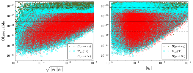
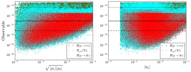
Figure 4: Rates for CLFV processes involving muons as a function of $|\eta_{1}|$ (right) and $\sqrt{|\rho_{1}||\rho_{2}|}$ (left panel). The upper (lower) panels are for a normal (inverted) hierarchy in the neutrino spectrum. The dotted, solid and dashed horizontal lines represent the sensitivity limit expected for the future searches for $\mathcal{B}(\mu\rightarrow e\gamma)$, $\mathcal{B}(\mu\rightarrow 3e)$ and $\mathcal{R}_{\mu e}$, respectively.

With respect to the CLFV observables we consider the current experimental bounds and their future expectations shown in Table 1, while for EDMs we have taken into account the current experimental limits $|d_{e}|\leqslant 8.7\times 10^{-29}{\rm\,e\,cm}$ Baron:2013eja , $|d_{\mu}|\leqslant 1.9\times 10^{-19}{\rm\,e\,cm}$ Bennett:2008dy and $|d_{\tau}|\leqslant 4.5\times 10^{-19}{\rm\,e\,cm}$ Inami:2002ah . Note that the strongest limit is set for the eEDM, and for that reason we do not display the muon and tau EDM results. In regard to future eEDM searches, it is worthwhile mentioning that the ACME collaboration will increase by two orders of magnitude the current bound Baron:2013eja ; futureACME .

Lastly, the parameters entering in the scalar potential are subject to the following perturbativity and vacuum stability constraints:

$$\mu_{1}^{2}<0,\;\;\mu_{2}^{2},\,\mu_{S}^{2}>0,\;\;|\mu|<500\,\text{GeV},\;\;\lambda_{1}\mu_{2}^{2}>\left(\lambda_{3}+\lambda_{4}\pm|\lambda_{5}|\right)\mu_{1}^{2},\;\;|\lambda_{S}|,\,|\lambda_{i}|<4\pi\;,$$

$$\lambda_{1},\,\lambda_{2},\,\lambda_{S}>0\;,\;\;\lambda_{6}>-\sqrt{\frac{\lambda_{1}\lambda_{S}}{2}}\;,\;\;\lambda_{7}>-\sqrt{\frac{\lambda_{2}\lambda_{S}}{2}}\;,\;\;\lambda_{3}+\lambda_{4}-|\lambda_{5}|+\sqrt{\lambda_{1}\lambda_{2}}>0\;.$$ (21)

Furthermore, we also impose the upper limits set by the perturbative unitarity of the $S$-matrix Ginzburg:2005dt ; Muhlleitner:2016mzt ; Liu:2017gfg ,

$$|\lambda_{3}\pm\lambda_{4}|\leq 8\pi,\,\,\,|\lambda_{3}\pm\lambda_{5}|\leq 8\pi,\,\,\,|\lambda_{3}+2\lambda_{4}\pm 3\lambda_{5}|\leq 8\pi,\,\,\,|\Lambda_{1}|,|\Lambda_{2}|,|\Lambda_{3}|\leq 8\pi,$$

$$\frac{1}{2}\left|\lambda_{1}+\lambda_{2}\pm\sqrt{(\lambda_{1}-\lambda_{2})^{2}+4\lambda_{4}^{2}}\right|\leq 8\pi,\,\,\,\frac{1}{2}\left|\lambda_{1}+\lambda_{2}\pm\sqrt{(\lambda_{1}-\lambda_{2})^{2}+4\lambda_{5}^{2}}\right|\leq 8\pi.$$ (22)

Here $\Lambda_{i}$ correspond to the three real eigenvalues of the matrix

$$\begin{pmatrix}3\lambda_{1}&2\lambda_{3}+\lambda_{4}&\sqrt{2}\lambda_{6}\\ 2\lambda_{3}+\lambda_{4}&3\lambda_{2}&\sqrt{2}\lambda_{7}\\ \sqrt{2}\lambda_{6}&\sqrt{2}\lambda_{7}&\lambda_{S}\end{pmatrix}.$$ (23)

All these theoretical conditions constrain the mass splittings among the $Z_{2}$-odd scalar particles.

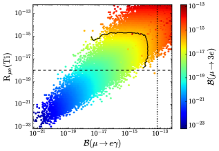
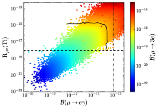
Figure 5: The available parameter space of the IZM and the future exclusion zones coming from the most constraining CLFV searches. Left (right) panel is for NH (IH). The dotted, solid and dashed lines represent the expected sensitivity for the future searches regarding $\mathcal{B}(\mu\rightarrow e\gamma)$, $\mathcal{B}(\mu\rightarrow 3e)$ and $\mathcal{R}_{\mu e}$, respectively.

In the following we present the results for the viable benchmark points obtained from the scan. Only the results for CLFV processes involving muon leptons in the inital state are displayed since the ones with tau leptons are out the reach of the forthcoming facilities. In Fig. 4 we display the dependence of the three observables $\mathcal{B}(\mu\rightarrow e\gamma)$ (green points), $\mathcal{R}_{\mu e}$ (cyan cross) and $\mathcal{B}(\mu\rightarrow 3e)$ (red dots) with $\sqrt{|\rho_{1}||\rho_{2}|}$ -the Yukawa couplings that are unconstrained by neutrino physics- (left panels) and with $\eta_{1}$ -the only free Yukawa coupling that enter in the neutrino mass generation- (right panels). From the results for the NH, the upper bounds $\sqrt{|\rho_{1}||\rho_{2}|}\lesssim 10^{-1}$ and $|\eta_{1}|\lesssim 10^{-2}$ are obtained. Note that the most constraining limits are those from $\mu-e$ conversion experiments, which will test Yukawa couplings down to $5\times 10^{-3}$. On the other hand, the results for inverted hierarchy give the upper bounds $|\eta_{1}|\lesssim 10^{-1}$ and $\sqrt{|\rho_{1}||\rho_{2}|}\lesssim 10^{-1}$, which may improve in around one order of magnitude in the future. The lower bound on $|\eta_{1}|$ that appears in the bottom right panel of Fig. 4 is due to the fact that for the IH the magnitude of the $\eta_{2,3}$ is less that $|\eta_{1}|$, which implies that for $|\eta_{1}|\approx 10^{-5}$ that value is excluded due to the lower limit imposed over all the Yukawa couplings. It is worth mentioning that the results for the three Yukawa couplings $\rho_{i}$ are similar for both neutrino mass spectrum since these couplings do not participate in the neutrino mass generation.

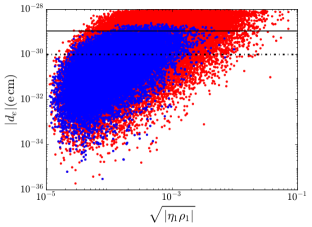
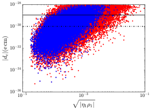
Figure 6: Expected values for the eEDM as a function of $\sqrt{|\eta_{1}\rho_{1}|}$ for NH (left panel) and IH (right panel). The red points constitute the current viable parameter space while the blue points are beyond the reach of future CLFV searches.

In Fig. 5 we show the correlation between the $\mathcal{B}(\mu\rightarrow e\gamma)$, $\mathcal{B}(\mu\rightarrow 3e)$ and $\mathcal{R}_{\mu e}$ observables, and the impact of the future searches associated to these observables over the parameter space considered. The correlation between the three observables is remarkable in a large portion of the parameter space. It follows that a large fraction of the current viable parameter space will be tested in the future experiments, with all the electron-muon observables being within the reach of the MEG and Mu3e experiments, and with the $\mathcal{R}_{\mu e}$ observable being the most promising.

The results for the eEDM as a function of the Yukawa coupling product $\sqrt{|\rho_{1}\eta_{1}|}$ are displayed in Fig. 6. Our results show that eEDM future searches Baron:2013eja (dashed lines) may test regions beyond the reach of experimental sensitivity of CLFV searches. Indeed, the most recent result on the eEDM from ACME collaboration Andreev:2018ayy has begun to test those regions (solid lines in Fig. 6). It turns out that these regions are precisely formed by benchmark points (for both neutrino mass spectrum) with $\mathcal{B}(\mu\to 3e)/\mathcal{B}(\mu\to e\gamma)>1$ and $\mathcal{R}_{\mu e}(\text{Ti})/\mathcal{B}(\mu\to e\gamma)\gtrsim 10$, that is, where the dipole contribution is not the dominant one. This means that, if it is experimentally observed that the above ratios are below the mentioned bounds, the parameter space we are considering would be disfavoured.

Finally, the contribution to the anomalous magnetic moment of the charged leptons are not so relevant since they are below the current bounds Patrignani:2016xqp . For completeness purposes we display in Fig. 7 the results for the anomalous magnetic moment of the muon. In particular, the new contribution is not enough to explain the discrepancy between the SM prediction and the experimental value $\Delta a_{\mu}=a_{\mu}^{\text{exp}}-a_{\mu}^{\text{SM}}=(288\pm 80)\times 10^{-11}$ Bennett:2006fi ; Patrignani:2016xqp .

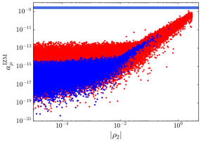
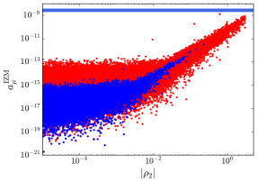
Figure 7: The new contribution $a_{\mu}^{\text{IZM}}$ to the anomalous magnetic dipole moment of the muon as a function of $|\rho_{2}|$ for NH (left panel) and IH (right panel). The horizontal blue band represents the discrepancy between the SM prediction and the experimental value Lindner:2016bgg .

V Conclusions

We have explored the inert Zee model in light of the ambitious experimental program designed to probe, via charged LFV processes and EDM signals, beyond the Standard Model scenarios. We determined the viable parameter space consistent with the current constraints coming from a diversity of directions: dark matter, neutrino oscillations, lepton flavor violating processes, electric dipole moments, electroweak precision tests and collider physics. We have also established the most relevant experimental perspectives regarding LFV searches, where we have found that $\mu-e$ conversion in muonic experiments constitutes the most promising way in this line of research. Furthermore, since the Yukawa couplings that reproduce the neutrino oscillation observables are complex, which in turn provide new sources of CP violation, we have shown the regions in the parameter space where the prospects for the eEDM are within the future experimental sensitivity. It is remarkable the impact that may have eEDM future searches since they may probe the model in regions out the reach of all the future CLFV projects.

Appendix A Loop functions

The analytical expressions for the loop functions involved in the $d_{\ell_{i}}$, $a_{\ell_{i}}$ and $\ell_{i}\to\ell_{j}\gamma$ observables are:

$$\mathcal{G}_{1}(m_{a}^{2},m_{b}^{2},m_{c}^{2}) =\frac{1}{m_{b}^{2}}G\left(\frac{m_{a}^{2}}{m_{b}^{2}}\right)-\frac{1}{m_{c}^{2}}G\left(\frac{m_{a}^{2}}{m_{c}^{2}}\right),$$ (24)

$$\mathcal{F}_{1}(m^{2}_{a},m_{b}^{2},m_{c}^{2}) =\frac{1}{2m_{a}^{2}}\left[F\left(\frac{m_{b}^{2}}{m_{a}^{2}}\right)+F\left(\frac{m_{c}^{2}}{m_{a}^{2}}\right)\right],$$ (25)

$$\mathcal{F}_{2}(m^{2}_{a},m_{b}^{2}) =\mathcal{F}_{1}(m_{a}^{2},m_{b}^{2},m_{b}^{2}),$$ (26)

$$\mathcal{I}_{1}(m_{a}^{2},m_{b}^{2},m_{c}^{2}) =\frac{1}{m_{a}^{2}}\left[G_{2}\left(\frac{m^{2}_{b}}{m^{2}_{a}}\right)-G_{2}\left(\frac{m^{2}_{c}}{m^{2}_{a}}\right)\right],$$ (27)

$$\mathcal{H}_{1}(m_{a}^{2},m_{b}^{2},m_{c}^{2}) =\frac{1}{m_{a}^{2}}\left[F\left(\frac{m^{2}_{b}}{m^{2}_{a}}\right)-F\left(\frac{m^{2}_{c}}{m^{2}_{a}}\right)\right],$$ (28)

$$\mathcal{H}_{2}(m_{a}^{2},m_{b}^{2}) =\mathcal{H}_{1}(m_{a}^{2},m_{b}^{2},0)=\frac{1}{m_{a}^{2}}F\left(\frac{m^{2}_{b}}{m^{2}_{a}}\right),$$ (29)

where

$$F\left(x\right) =\frac{2x^{3}+3x^{2}-6x+1-6x^{2}\log\left(x\right)}{6\left(x-1\right)^{4}},$$ (30)

$$G\left(x\right) =\frac{x^{2}-4x+3+2\log\left(x\right)}{2\left(x-1\right)^{3}},$$ (31)

$$G_{2}(x) =\frac{3x^{2}-4x+1-2x^{2}\mbox{log}(x)}{2(1-x)^{3}}.$$ (32)

References

- (1) Super-Kamiokande Collaboration, Y. Fukuda et al., Phys.Rev.Lett. 81, 1562 (1998), arXiv:hep-ex/9807003.
- (2) SNO Collaboration, Q. Ahmad et al., Phys.Rev.Lett. 89, 011301 (2002), arXiv:nucl-ex/0204008.
- (3) M. Lindner, M. Platscher, and F. S. Queiroz, Phys. Rept. 731, 1 (2018), arXiv:1610.06587.
- (4) L. Calibbi and G. Signorelli, Riv. Nuovo Cim. 41, 1 (2018), arXiv:1709.00294.
- (5) MEG Collaboration, J. Adam et al., Phys.Rev.Lett. 110, 201801 (2013), arXiv:1303.0754.
- (6) A. Baldini et al., (2013), arXiv:1301.7225.
- (7) SINDRUM Collaboration, U. Bellgardt et al., Nucl.Phys. B299, 1 (1988).
- (8) A. Blondel et al., (2013), arXiv:1301.6113.
- (9) Mu2e, R. M. Carey et al., (2008).
- (10) Mu2e, D. Glenzinski, AIP Conf.Proc. 1222, 383 (2010).
- (11) Mu2e, R. Abrams et al., (2012), arXiv:1211.7019.
- (12) DeeMe, M. Aoki, PoS ICHEP2010, 279 (2010).
- (13) DeeMe, H. Natori, Nucl. Phys. Proc. Suppl. 248-250, 52 (2014).
- (14) COMET, Y. G. Cui et al., (2009).
- (15) COMET, Y. Kuno, PTEP 2013, 022C01 (2013).
- (16) R. J. Barlow, Nucl. Phys. Proc. Suppl. 218, 44 (2011).
- (17) D. M. Kara et al., New J. Phys. 14, 103051 (2012), arXiv:1208.4507.
- (18) D. Kawall, J. Phys. Conf. Ser. 295, 012031 (2011).
- (19) ACME, J. Baron et al., Science 343, 269 (2014), arXiv:1310.7534.
- (20) Particle Data Group, C. Patrignani et al., Chin. Phys. C40, 100001 (2016).
- (21) P. F. de Salas, D. V. Forero, C. A. Ternes, M. Tortola, and J. W. F. Valle, Phys. Lett. B782, 633 (2018), arXiv:1708.01186.
- (22) Y. Cai, J. Herrero-García, M. A. Schmidt, A. Vicente, and R. R. Volkas, Front.in Phys. 5, 63 (2017), arXiv:1706.08524.
- (23) V. Brdar, I. Picek, and B. Radovcic, Phys. Lett. B728, 198 (2014), arXiv:1310.3183.
- (24) D. Restrepo, O. Zapata, and C. E. Yaguna, JHEP 1311, 011 (2013), arXiv:1308.3655.
- (25) C.-S. Chen, K. L. McDonald, and S. Nasri, Phys. Lett. B734, 388 (2014), arXiv:1404.6033.
- (26) A. Ahriche, A. Manning, K. L. McDonald, and S. Nasri, Phys. Rev. D94, 053005 (2016), arXiv:1604.05995.
- (27) C. Simoes and D. Wegman, JHEP 04, 148 (2017), arXiv:1702.04759.
- (28) C.-Y. Yao and G.-J. Ding, Phys. Rev. D96, 095004 (2017), arXiv:1707.09786.
- (29) C.-Y. Yao and G.-J. Ding, Phys. Rev. D97, 095042 (2018), arXiv:1802.05231.
- (30) A. Zee, Phys.Lett. B93, 389 (1980).
- (31) L. Wolfenstein, Nucl. Phys. B175, 93 (1980).
- (32) S. T. Petcov, Phys. Lett. 115B, 401 (1982).
- (33) T. Toma and A. Vicente, JHEP 1401, 160 (2014), arXiv:1312.2840.
- (34) A. Vicente and C. E. Yaguna, JHEP 02, 144 (2015), arXiv:1412.2545.
- (35) T. A. Chowdhury and S. Nasri, JHEP 12, 040 (2015), arXiv:1506.00261.
- (36) Y. Cai and M. A. Schmidt, JHEP 05, 028 (2016), arXiv:1603.00255.
- (37) P. Rocha-Moran and A. Vicente, JHEP 07, 078 (2016), arXiv:1605.01915.
- (38) S. Esch, M. Klasen, D. R. Lamprea, and C. E. Yaguna, Eur. Phys. J. C78, 88 (2018), arXiv:1602.05137.
- (39) A. Abada and T. Toma, JHEP 04, 030 (2018), arXiv:1802.00007.
- (40) S. Esch, M. Klasen, and C. E. Yaguna, (2018), arXiv:1804.03384.
- (41) R. Barbieri, L. J. Hall, and V. S. Rychkov, Phys.Rev. D74, 015007 (2006), arXiv:hep-ph/0603188.
- (42) L. Lopez Honorez, E. Nezri, J. F. Oliver, and M. H. Tytgat, JCAP 0702, 028 (2007), arXiv:hep-ph/0612275.
- (43) L. Lopez Honorez and C. E. Yaguna, JHEP 09, 046 (2010), arXiv:1003.3125.
- (44) L. Lopez Honorez and C. E. Yaguna, JCAP 1101, 002 (2011), arXiv:1011.1411.
- (45) A. Goudelis, B. Herrmann, and O. Stål, JHEP 09, 106 (2013), arXiv:1303.3010.
- (46) C. Garcia-Cely and A. Ibarra, JCAP 1309, 025 (2013), arXiv:1306.4681.
- (47) A. Arhrib, Y.-L. S. Tsai, Q. Yuan, and T.-C. Yuan, JCAP 1406, 030 (2014), arXiv:1310.0358.
- (48) E. Ma, Phys.Rev. D73, 077301 (2006), arXiv:hep-ph/0601225.
- (49) Y. Bai and J. Berger, JHEP 08, 153 (2014), arXiv:1402.6696.
- (50) J. Kile, A. Kobach, and A. Soni, Phys. Lett. B744, 330 (2015), arXiv:1411.1407.
- (51) M.-C. Chen, J. Huang, and V. Takhistov, JHEP 02, 060 (2016), arXiv:1510.04694.
- (52) K. Kowalska and E. M. Sessolo, JHEP 09, 112 (2017), arXiv:1707.00753.
- (53) L. Calibbi, R. Ziegler, and J. Zupan, JHEP 07, 046 (2018), arXiv:1804.00009.
- (54) R. Longas, D. Portillo, D. Restrepo, and O. Zapata, JHEP 03, 162 (2016), arXiv:1511.01873.
- (55) M. Kadastik, K. Kannike, and M. Raidal, Phys. Rev. D81, 015002 (2010), arXiv:0903.2475.
- (56) M. Kadastik, K. Kannike, and M. Raidal, Phys. Rev. D80, 085020 (2009), arXiv:0907.1894, [Erratum: Phys. Rev.D81,029903(2010)].
- (57) M. Kakizaki, A. Santa, and O. Seto, Int. J. Mod. Phys. A32, 1750038 (2017), arXiv:1609.06555.
- (58) X. Liu and L. Bian, Phys. Rev. D97, 055028 (2018), arXiv:1706.06042.
- (59) C.-Y. Chen, M. Freid, and M. Sher, Phys. Rev. D89, 075009 (2014), arXiv:1312.3949.
- (60) M. Muhlleitner, M. O. P. Sampaio, R. Santos, and J. Wittbrodt, JHEP 03, 094 (2017), arXiv:1612.01309.
- (61) W. Rodejohann and J. W. F. Valle, Phys. Rev. D84, 073011 (2011), arXiv:1108.3484.
- (62) M. Reig, D. Restrepo, J. W. F. Valle, and O. Zapata, (2018), arXiv:1806.09977.
- (63) Particle Data Group, K. A. Olive et al., Chin. Phys. C38, 090001 (2014).
- (64) W. Porod, F. Staub, and A. Vicente, Eur. Phys. J. C74, 2992 (2014), arXiv:1405.1434.
- (65) BaBar Collaboration, B. Aubert et al., Phys.Rev.Lett. 104, 021802 (2010), arXiv:0908.2381.
- (66) SuperB, M. Bona et al., (2007), arXiv:0709.0451.
- (67) Belle, Y. Miyazaki et al., Phys. Lett. B719, 346 (2013), arXiv:1206.5595.
- (68) T. Aushev et al., (2010), arXiv:1002.5012.
- (69) K. Hayasaka et al., Phys. Lett. B687, 139 (2010), arXiv:1001.3221.
- (70) SINDRUM II, C. Dohmen et al., Phys. Lett. B317, 631 (1993).
- (71) SINDRUM II, W. H. Bertl et al., Eur. Phys. J. C47, 337 (2006).
- (72) W. Porod, Comput. Phys. Commun. 153, 275 (2003), arXiv:hep-ph/0301101.
- (73) W. Porod and F. Staub, Comput. Phys. Commun. 183, 2458 (2012), arXiv:1104.1573.
- (74) F. Staub, Comput. Phys. Commun. 185, 1773 (2014), arXiv:1309.7223.
- (75) F. Staub, Adv. High Energy Phys. 2015, 840780 (2015), arXiv:1503.04200.
- (76) G. Belanger, F. Boudjema, A. Pukhov, and A. Semenov, (2013), arXiv:1305.0237.
- (77) Planck, P. A. R. Ade et al., Astron. Astrophys. 594, A13 (2016), arXiv:1502.01589.
- (78) Gfitter Group, M. Baak et al., Eur.Phys.J. C74, 3046 (2014), arXiv:1407.3792.
- (79) L3, P. Achard et al., Phys. Lett. B517, 75 (2001), arXiv:hep-ex/0107015.
- (80) E. Lundstrom, M. Gustafsson, and J. Edsjo, Phys.Rev. D79, 035013 (2009), arXiv:0810.3924.
- (81) G. Belanger et al., Phys. Rev. D91, 115011 (2015), arXiv:1503.07367.
- (82) A. Ilnicka, M. Krawczyk, and T. Robens, (2015), arXiv:1508.01671.
- (83) ATLAS, M. Aaboud et al., Phys. Rev. D98, 052005 (2018), arXiv:1802.04146.
- (84) CMS, A. M. Sirunyan et al., (2018), arXiv:1804.02716.
- (85) Muon (g-2), G. W. Bennett et al., Phys. Rev. D80, 052008 (2009), arXiv:0811.1207.
- (86) Belle, K. Inami et al., Phys. Lett. B551, 16 (2003), arXiv:hep-ex/0210066.
- (87) W. C. Griffith, Plenary talk ”at interplay between particle & astroparticle physics 2014”, in https://indico.ph.qmul.ac.uk/indico/conferenceDisplay.py?confId=1, 2014.
- (88) I. F. Ginzburg and I. P. Ivanov, Phys. Rev. D72, 115010 (2005), arXiv:hep-ph/0508020.
- (89) ACME, V. Andreev et al., Nature 562, 355 (2018).
- (90) Muon g-2, G. W. Bennett et al., Phys. Rev. D73, 072003 (2006), arXiv:hep-ex/0602035.