Towards Dynamic Computation Graphs via Sparse Latent Structure

Abstract

Deep NLP models benefit from underlying structures in the data—e.g., parse trees—typically extracted using off-the-shelf parsers. Recent attempts to jointly learn the latent structure encounter a tradeoff: either make factorization assumptions that limit expressiveness, or sacrifice end-to-end differentiability. Using the recently proposed $\operatorname*{\mathsf{SparseMAP}}$ inference, which retrieves a sparse distribution over latent structures, we propose a novel approach for end-to-end learning of latent structure predictors jointly with a downstream predictor. To the best of our knowledge, our method is the first to enable unrestricted dynamic computation graph construction from the global latent structure, while maintaining differentiability.

1 Introduction

Latent structure models are a powerful tool for modeling compositional data and building NLP pipelines Smith (2011). An interesting emerging direction is to dynamically adapt a network’s computation graph, based on structure inferred from the input; notable applications include learning to write programs Bosnjak et al. (2017), answering visual questions by composing specialized modules Hu et al. (2017); Johnson et al. (2017), and composing sentence representations using latent syntactic parse trees Yogatama et al. (2017).

But how to learn a model that is able to condition on such combinatorial variables? The question then becomes: how to marginalize over all possible latent structures? For tractability, existing approaches have to make a choice. Some of them eschew global latent structure, resorting to computation graphs built from smaller local decisions: e.g., structured attention networks use local posterior marginals as attention weights Kim et al. (2017); Liu and Lapata (2018), and Maillard et al. (2017) construct sentence representations from parser chart entries. Others allow more flexibility at the cost of losing end-to-end differentiability, ending up with reinforcement learning problems Yogatama et al. (2017); Hu et al. (2017); Johnson et al. (2017); Williams et al. (2018). More traditional approaches employ an off-line structure predictor (e.g., a parser) to define the computation graph Tai et al. (2015); Chen et al. (2017), sometimes with some parameter sharing Bowman et al. (2016). However, these off-line methods are unable to jointly train the latent model and the downstream classifier via error gradient information.

We propose here a new strategy for building dynamic computation graphs with latent structure, through sparse structure prediction. Sparsity allows selecting and conditioning on a tractable number of global structures, eliminating the limitations stated above. Namely, our approach is the first that:

• is fully differentiable;

• supports latent structured variables;

• can marginalize over full global structures.

This contrasts with off-line and with reinforcement learning-based approaches, which satisfy B and C but not A; and with local marginal-based methods such as structured attention networks, which satisfy A and B, but not C. Key to our approach is the recently proposed $\operatorname*{\mathsf{SparseMAP}}$ inference Niculae et al. (2018), which induces, for each data example, a very sparse posterior distribution over the possible structures, allowing us to compute the expected network output efficiently and explicitly in terms of a small, interpretable set of latent structures. Our model can be trained end-to-end with gradient-based methods, without the need for policy exploration or sampling.

We demonstrate our strategy on inducing latent dependency TreeLSTMs, achieving competitive results on sentence classification, natural language inference, and reverse dictionary lookup.

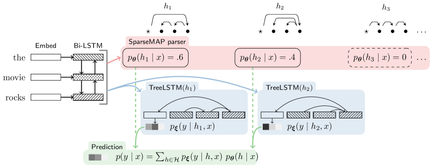
Figure 1: Our method computes a sparse probability distribution over all possible latent structures: here, only two have nonzero probability. For each selected tree $h$, we evaluate $p_{\bm{\xi}}(y\mid h,x)$ by dynamically building the corresponding computation graph (e.g., a TreeLSTM). The final, posterior prediction is a sparse weighted average.

2 Sparse Latent Structure Prediction

We describe our proposed approach for learning with combinatorial structures (in particular, non-projective dependency trees) as latent variables.

2.1 Latent Structure Models

Let $x$ and $y$ denote classifier inputs and outputs, and $h\in\mathcal{H}(x)$ a latent variable; for example, $\mathcal{H}(x)$ can be the set of possible dependency trees for $x$. We would like to train a neural network to model

$$p(y\mid x)\coloneqq\sum_{h\in\mathcal{H}(x)}p_{\bm{\theta}}(h\mid x)\,p_{\bm{\xi}}(y\mid h,x),$$ (1)

where $p_{\bm{\theta}}(h\mid x)$ is a structured-output parsing model that defines a distribution over trees, and $p_{\bm{\xi}}(y\mid h,x)$ is a classifier whose computation graph may depend freely and globally on the structure $h$ (e.g., a TreeLSTM). The rest of this section focuses on the challenge of defining $p_{\bm{\theta}}(h\mid x)$ such that Eqn. 1 remains tractable and differentiable.

2.2 Global Inference

Denote by $f_{\bm{\theta}}(h;\,x)$ a scoring function, assigning each tree a non-normalized score. For instance, we may have an arc-factored score $f_{\bm{\theta}}(h;x)\coloneqq\sum_{a\in h}s_{\bm{\theta}}(a;x)$, where we interpret a tree $h$ as a set of directed arcs $a$, each receiving an atomic score $s_{\bm{\theta}}(a;x)$. Deriving $p_{\bm{\theta}}$ given $f_{\bm{\theta}}$ is known as structured inference. This can be written as a $\Omega$-regularized optimization problem of the form

$$p_{\bm{\theta}}(\cdot\mid x)\coloneqq\operatorname*{\mathsf{argmax}}_{q\in\triangle^{|\mathcal{H}(x)|}}\sum_{h\in\mathcal{H}(x)}q(h)f_{\bm{\theta}}(h;x)-\Omega(q),$$

where $\triangle^{|\mathcal{H}(x)|}$ is the set of all possible probability distributions over $\mathcal{H}(x)$. Examples follow.

Marginal inference.

With negative entropy regularization, i.e., $\Omega(q)\coloneqq\sum_{h\in\mathcal{H}(x)}q(h)\mathop{\mathsf{log}}\displaylimits q(h)$, we recover marginal inference, and the probability of a tree becomes (Wainwright and Jordan, 2008)

$$p_{\bm{\theta}}(h\mid x)\propto\mathop{\mathsf{exp}}\displaylimits(f_{\bm{\theta}}(h;x)).$$

This closed-form derivation, detailed in Appendix A, provides a differentiable expression for $p_{\bm{\theta}}$. However, crucially, since $\mathop{\mathsf{exp}}\displaylimits(\cdot)>0$, every tree is assigned strictly nonzero probability. Therefore—unless the downstream $p_{\bm{\xi}}$ is constrained to also factor over arcs, as in Kim et al. (2017); Liu and Lapata (2018)—the sum in Eqn. 1 requires enumerating the exponentially large $\mathcal{H}(x)$. This is generally intractable, and even hard to approximate via sampling, even when $p_{\bm{\theta}}$ is tractable.

$\operatorname*{\mathsf{MAP}}$ inference.

At the polar opposite, setting $\Omega(q)\coloneqq 0$ yields maximum a posteriori ($\operatorname*{\mathsf{MAP}}$) inference (see Appendix A). $\operatorname*{\mathsf{MAP}}$ assigns a probability of $1$ to the highest-scoring tree, and $0$ to all others, yielding a very sparse $p_{\bm{\theta}}$. However, since the top-scoring tree (or top-$k$, for fixed $k$) does not vary with small changes in ${\bm{\theta}}$, error gradients cannot propagate through $\operatorname*{\mathsf{MAP}}$. This prevents end-to-end gradient-based training for $\operatorname*{\mathsf{MAP}}$-based latent variables, which makes them more difficult to use. Related reinforcement learning approaches also yield only one structure, but sidestep non-differentiability by instead introducing more challenging search problems.

2.3 Sparse Inference

In this work, we propose using $\operatorname*{\mathsf{SparseMAP}}$ inference (Niculae et al., 2018) to sparsify the set $\mathcal{H}$ while preserving differentiability. $\operatorname*{\mathsf{SparseMAP}}$ uses a quadratic penalty on the posterior marginals

$$\Omega(q)\coloneqq\left\lVert\bm{u}(q)\right\rVert_{2}^{2},~{}~{}\text{where}~{}~{}\left[\bm{u}(q)\right]_{a}\coloneqq\sum_{h:a\in h}q(h).$$

Situated between marginal inference and $\operatorname*{\mathsf{MAP}}$ inference, $\operatorname*{\mathsf{SparseMAP}}$ assigns nonzero probability to only a small set of plausible trees $\bar{\mathcal{H}}\subset\mathcal{H}$, of size at most equal to the number of arcs (Martins et al., 2015, Proposition 11). This guarantees that the summation in Eqn. 1 can be computed efficiently by iterating over $\bar{\mathcal{H}}$: this is depicted in Figure 1 and described in the next paragraphs.

Forward pass.

To compute $p(y\mid x)$ (Eqn. 1), we observe that the $\operatorname*{\mathsf{SparseMAP}}$ posterior $p_{\bm{\theta}}$ is nonzero only on a small set of trees $\bar{\mathcal{H}}$, and thus we only need to compute $p_{\bm{\xi}}(y\mid h,x)$ for $h\in\bar{\mathcal{H}}$. The support and values of $p_{\bm{\theta}}$ are obtained by solving the $\operatorname*{\mathsf{SparseMAP}}$ inference problem, as we describe in Niculae et al. (2018). The strategy, based on the active set algorithm (Nocedal and Wright, 1999, chapter 16), involves a sequence of $\operatorname*{\mathsf{MAP}}$ calls (here: maximum spanning tree problems.)

Backward pass.

We next show how to compute end-to-end gradients efficiently. Recall from Eqn. 1 $p(y\mid x)=\sum_{h\in\mathcal{H}}p_{\bm{\theta}}(h\mid x)\,p_{\bm{\xi}}(y\mid h,x),$ where $h$ is a discrete index of a tree. To train the classifier, we have $\nicefrac{{\partial p(y\mid x)}}{{\partial{\bm{\xi}}}}=\sum_{h\in\mathcal{H}}p_{\bm{\theta}}(h\mid x)\nicefrac{{\partial p_{\bm{\xi}}(y\mid h,x)}}{{\partial{\bm{\xi}}}}$, therefore only the terms with nonzero probability (i.e., $h\in\bar{\mathcal{H}}$) contribute to the gradient. $\nicefrac{{\partial p_{\bm{\xi}}(y\mid h,x)}}{{\partial{\bm{\xi}}}}$ is readily available by implementing $p_{\bm{\xi}}$ in an automatic differentiation library. To train the latent parser, the total gradient $\nicefrac{{\partial p(y\mid x)}}{{{\bm{\theta}}}}$ is the sum $\sum_{h\in\bar{\mathcal{H}}}p_{\bm{\xi}}(y\mid h,x)~{}\nicefrac{{\partial p_{\bm{\theta}}(h\mid x)}}{{\partial{\bm{\theta}}}}.$ We derive the expression of $\nicefrac{{\partial p_{\bm{\theta}}(h\mid x)}}{{\partial{\bm{\theta}}}}$ in Appendix B. Crucially, the gradient sum is also sparse, like $p_{\bm{\theta}}$, and efficient to compute, amounting to multiplying by a $|\bar{\mathcal{H}}(x)|$-by-$|\bar{\mathcal{H}}(x)|$ matrix. The proof, given in Appendix B, is a novel extension of the $\operatorname*{\mathsf{SparseMAP}}$ backward pass (Niculae et al., 2018).

Generality.

Our description focuses on probabilistic classifiers, but our method can be readily applied to networks that output any representation, not necessarily a probability. For this, we define a function $\bm{r}_{\bm{\xi}}(h,x)$, consisting of any auto-differentiable computation w.r.t. $x$, conditioned on the discrete latent structure $h$ in arbitrary, non-differentiable ways. We then compute

$$\bar{\bm{r}}(x)\coloneqq\sum_{h\in\mathcal{H}(x)}p_{\bm{\theta}}(h\mid x)\bm{r}_{\bm{\xi}}(h,x)\\ =\mathbb{E}_{h\sim p_{\bm{\theta}}}\bm{r}_{\bm{\xi}}(h,x).$$

This strategy is demonstrated in our reverse-dictionary experiments in §3.4. In addition, our approach is not limited to trees: any structured model with tractable $\operatorname*{\mathsf{MAP}}$ inference may be used.

3 Experiments

	subj.	SST	SNLI
left-to-right	92.71	82.10	80.98
flat	92.56	83.96	81.74
off-line	92.15	83.25	81.37
latent	92.25	84.73	81.87

Table 1: Accuracy scores for classification and NLI.

	seen			unseen			concepts
	rank	acc10	acc100	rank	acc10	acc100	rank	acc10	acc100
left-to-right	17	42.6	73.8	43	33.2	61.8	28	35.9	66.7
flat	18	45.1	71.1	31	38.2	65.6	29	34.3	68.2
latent	12	47.5	74.6	40	35.6	60.1	20	38.4	70.7
Maillard et al. (2017)	58	30.9	56.1	40	33.4	57.1	40	57.1	62.6
Hill et al. (2016)	12	48	28	22	41	70	69	28	54

Table 2: Results on the reverse dictionary lookup task Hill et al. (2016). Following the authors, for an input definition, we rank a shortlist of approximately 50k candidate words according to the cosine similarity to the output vector, and report median rank of the expected word, accuracy at 10, and at 100.

We evaluate our approach on three natural language processing tasks: sentence classification, natural language inference, and reverse dictionary lookup.

3.1 Common aspects

Word vectors.

Unless otherwise mentioned, we initialize with 300-dimensional GloVe word embeddings Pennington et al. (2014) We transform every sentence via a bidirectional LSTM encoder, to produce a context-aware vector $\bm{v}_{i}$ encoding word $i$.

Dependency TreeLSTM.

We combine the word vectors $\bm{v}_{i}$ in a sentence into a single vector using a tree-structured Child-Sum LSTM, which allows an arbitrary number of children at any node Tai et al. (2015). Our baselines consist in extreme cases of dependency trees: where the parent of word $i$ is word $i+1$ (resulting in a left-to-right sequential LSTM), and where all words are direct children of the root node (resulting in a flat additive model). We also consider off-line dependency trees precomputed by Stanford CoreNLP Manning et al. (2014).

Neural arc-factored dependency parsing.

We compute arc scores $s_{\bm{\theta}}(a;x)$ with one-hidden-layer perceptrons Kiperwasser and Goldberg (2016).

Experimental setup.

All networks are trained via stochastic gradient with 16 samples per batch. We tune the learning rate on a log-grid, using a decay factor of $0.9$ after every epoch at which the validation performance is not the best seen, and stop after five epochs without improvement. At test time, we scale the arc scores $s_{\bm{\theta}}$ by a temperature $t$ chosen on the validation set, controlling the sparsity of the $\operatorname*{\mathsf{SparseMAP}}$ distribution. All hidden layers are $300$-dimensional.

3.2 Sentence classification

We evaluate our models for sentence-level subjectivity classification Pang and Lee (2004) and for binary sentiment classification on the Stanford Sentiment Treebank Socher et al. (2013). In both cases, we use a softmax output layer on top of the Dependency TreeLSTM output representation.

3.3 Natural language inference (NLI)

We apply our strategy to the SNLI corpus Bowman et al. (2015), which consists of classifying premise-hypothesis sentence pairs into entailment, contradiction or neutral relations. In this case, for each pair ($x_{P},x_{H}$), the running sum is over two latent distributions over parse trees, i.e., $\sum_{h_{P}\in\mathcal{H}(x_{P})}\sum_{h_{H}\in\mathcal{H}(x_{H})}p_{\bm{\xi}}(y\mid x_{\{P,H\}},h_{\{P,H\}})\\ p_{\bm{\theta}}(h_{P}\mid x_{P})p_{\bm{\theta}}(h_{H}\mid x_{H}).$ For each pair of trees, we independently encode the premise and hypothesis using a TreeLSTM. We then concatenate the two vectors, their difference, and their element-wise product Mou et al. (2016). The result is passed through one tanh hidden layer, followed by the softmax output layer.

3.4 Reverse dictionary lookup

The reverse dictionary task aims to compose a dictionary definition into an embedding that is close to the defined word. We therefore used fixed input and output embeddings, set to unit-norm 500-dimensional vectors provided, together with training and evaluation data, by Hill et al. (2016). The network output is a projection of the TreeLSTM encoding back to the dimension of the word embeddings, normalized to unit $\ell_{2}$ norm. We maximize the cosine similarity of the predicted vector with the embedding of the defined word.

28% [hide label,edge unit distance=1.1ex] [column sep=0.4cm] $\star$ & a & vivid & cinematic & portrait & .
121.0 131.0 141.0 151.0 161.0
✓ 16% [hide label,edge unit distance=1.1ex] [column sep=0.4cm] $\star$ & a & vivid & cinematic & portrait & .
521.0 531.0 541.0 151.0 561.0
$\cdots$
13%

[hide label,edge unit distance=1.1ex] [column sep=0.4cm] $\star$ & a & vivid & cinematic & portrait & .
421.0 431.0 641.0 451.0 [edge unit distance=0.8ex]161.0
$\cdots$

Figure 2: Three of the sixteen trees with nonzero probability for an SST test example. Flat representations, such as the first tree, perform well on this task, as reflected by the baselines. The second tree, marked with ✓, agrees with the off-line parser.

† 22.6%

[hide label,edge unit distance=1.1ex] [column sep=0.3cm] $\star$ & lovely & and & poignant & .

321.0 131.0 341.0 351.0

✓ 21.4%

[hide label,edge unit distance=1.1ex] [column sep=0.3cm] $\star$ & lovely & and & poignant & .

121.0 231.0 241.0 251.0

19.84%

[hide label,edge unit distance=1.1ex] [column sep=0.3cm] $\star$ & lovely & and & poignant & .

421.0 431.0 141.0 451.0

$\cdots$

15.33%

[hide label,edge unit distance=1.1ex] [column sep=0.3cm] $\star$ & a & deep & and & meaningful & film & .

121.0 131.0 141.0 151.0 161.0 171.0

† 15.27%

[hide label,edge unit distance=1.1ex] [column sep=0.3cm] $\star$ & a & deep & and & meaningful & film & .

421.0 431.0 141.0 451.0 461.0 471.0

$\cdots$

✓ 0%

[hide label,edge unit distance=1.1ex] [column sep=0.3cm] $\star$ & a & deep & and & meaningful & film & .

621.0 631.0 341.0 351.0 161.0 671.0

Figure 3: Examples of coordinate structures where our model assigns high probability to a symmetric parse (marked †). While not consistent with the standard asymmetrical parse produced by CoreNLP (marked with ✓), the symmetric analysis may be more appropriate for TreeLSTM composition.

4 Discussion

Experimental performance.

Classification and NLI results are reported in Table 1. Compared to the latent structure model of Yogatama et al. (2017), our model performs better on SNLI (80.5%) but worse on SST (86.5%). On SNLI, our model also outperforms Maillard et al. (2017) (81.6%). To our knowledge, latent structure models have not been tested on subjectivity classification. Surprisingly, the simple flat and left-to-right baselines are very strong, outperforming the off-line dependency tree models on all three datasets. The latent TreeLSTM model reaches the best accuracy on two out of the three datasets. On reverse dictionary lookup (Table 2), our model also performs well, especially on concept classification, where the input definitions are more different from the ones seen during training. For context, we repeat the scores of the CKY-based latent TreeLSTM model of Maillard et al. (2017), as well as of the LSTM from Hill et al. (2016); these different-sized models are not entirely comparable. We attribute our model’s performance to the latent parser’s flexibility, investigated below.

Selected latent structures.

We analyze the latent structures selected by our model on SST, where the flat composition baseline is remarkably strong. We find that our model, to maximize accuracy, prefers flat or nearly-flat trees, but not exclusively: the average posterior probability of the flat tree is 28.9%. In Figure 2, the highest-ranked tree is flat, but deeper trees are also selected, including the projective CoreNLP parser output. Syntax is not necessarily an optimal composition order for a latent TreeLSTM, as illustrated by the poor performance of the off-line parser (Table 1). Consequently, our (fully unsupervised) latent structures tend to disagree with CoreNLP: the average probability of CoreNLP arcs is 5.8%; Williams et al. (2018) make related observations. Indeed, some syntactic conventions may be questionable for recursive composition. Figure 3 shows two examples where our model identifies a plausible symmetric composition order for coordinate structures: this analysis disagrees with CoreNLP, which uses the asymmetrical Stanford / UD convention of assigning the left-most conjunct as head (Nivre et al., 2016). Assigning the conjunction as head instead seems preferable in a Child-Sum TreeLSTM.

Training efficiency.

Our model must evaluate at least one TreeLSTM for each sentence, making it necessarily slower than the baselines, which evaluate exactly one. Thanks to sparsity and auto-batching, the actual slow-down is not problematic; moreover, as the model trains, the latent parser gets more confident, and for many unambiguous sentences there may be only one latent tree with nonzero probability. On SST, our average training epoch is only 4.7$\times$ slower than the off-line parser and 6$\times$ slower than the flat baseline.

5 Conclusions and future work

We presented a novel approach for training latent structure neural models, based on the key idea of sparsifying the set of possible structures, and demonstrated our method with competitive latent dependency TreeLSTM models. Our method’s generality opens up several avenues for future work: since it supports any structure for which $\operatorname*{\mathsf{MAP}}$ inference is available (e.g., matchings, alignments), and we have no restrictions on the downstream $p_{\bm{\xi}}(y\mid h,x)$, we may design latent versions of more complicated state-of-the-art models, such as ESIM for NLI Chen et al. (2017). In concurrent work, Peng et al. (2018) proposed an approximate $\operatorname*{\mathsf{MAP}}$ backward pass, relying on a relaxation and a gradient projection. Unlike our method, theirs does not support multiple latent structures; we intend to further study the relationship between the methods.

Supplementary Material

Appendix A Variational formulations of marginal and MAP inference.

In this section, we provide a brief explanation of the known result that marginal and $\operatorname*{\mathsf{MAP}}$ inference can be expressed as optimization problems of the form

$$p_{\bm{\theta}}(\cdot\mid x)\coloneqq\operatorname*{\mathsf{argmax}}_{q\in\triangle^{|\mathcal{H}(x)|}}\sum_{h\in\mathcal{H}(x)}q(h)f_{\bm{\theta}}(h;x)-\Omega(q),$$ (2)

where $\triangle^{|\mathcal{H}(x)|}$ is the set of all possible probability distributions over $\mathcal{H}(x)$, i.e., $\triangle^{|\mathcal{H}(x)|}\coloneqq\{q\in\mathbb{R}^{|\mathcal{H}(x)|}\colon\sum_{i=1}^{|\mathcal{H}(x)|}q_{i}=1,\text{ and }q_{i}\geq 0~{}\forall~{}i\}$.

Marginal inference.

We set $\Omega(q)\coloneqq\sum_{h\in\mathcal{H}(x)}q(h)\mathop{\mathsf{log}}\displaylimits q(h)$, i.e., the negative Shannon entropy (with base $e$). The resulting problem is well-studied (Boyd and Vandenberghe, 2004, Example 3.25). Its Lagrangian is

$$\mathcal{L}(q,\mu,\tau)=\sum_{h\in\mathcal{H}(x)}\bigl{(}q(h)\mathop{\mathsf{log}}\displaylimits q(h)-q(h)(f_{\bm{\theta}}(h;x)+\mu(h))\bigr{)}-\tau\bigl{(}1-\sum_{h\in\mathcal{H}(x)}q(h)\bigr{)}.$$ (3)

The KKT conditions for optimality are

$$\nabla\mathcal{L}(q,\mu,\tau) =0$$ (4)

$$q(h)\mu(h) =0\quad\forall h\in\mathcal{H}(x)$$

$$\mu(h) \geq 0$$

$$\sum_{h\in\mathcal{H}(x)}q(h) =1$$

The gradient takes the form

$$\nabla_{q(h)}\mathcal{L}(q,\mu,\tau)=1+\mathop{\mathsf{log}}\displaylimits q(h)-f_{\bm{\theta}}(h;x)-\mu(h)+\tau,$$ (5)

and setting $\nabla\mathcal{L}(q,\mu,\tau)=0$ yields the condition

$$\mathop{\mathsf{log}}\displaylimits q(h)=f_{\bm{\theta}}(h;x)+\mu(h)-\tau-1.$$ (6)

The above implies $q(h)>0$, which, by complementary slackness, means $\mu(h)=0~{}\forall h\in\mathcal{H}(x)$. Therefore

$$q(h)=\mathop{\mathsf{exp}}\displaylimits\bigl{(}f_{\bm{\theta}}(h;x)-\tau-1\bigr{)}=\frac{\mathop{\mathsf{exp}}\displaylimits\bigl{(}f_{\bm{\theta}}(h;x)\bigr{)}}{Z}$$ (7)

where we introduced $Z\coloneqq\mathop{\mathsf{exp}}\displaylimits(\tau+1)>0$. From the primal feasibility condition, we have

$$1=\sum_{h\in\mathcal{H}(x)}q(h)=\frac{1}{Z}\sum_{h\in\mathcal{H}(x)}\mathop{\mathsf{exp}}\displaylimits\bigl{(}f_{\bm{\theta}}(h;x)\bigr{)},$$ (8)

and thus

$$Z=\sum_{h\in\mathcal{H}(x)}\mathop{\mathsf{exp}}\displaylimits\bigl{(}f_{\bm{\theta}}(h;x)\bigr{)},$$ (9)

yielding the desired result: $p_{\bm{\theta}}(h\mid x)=Z^{-1}\mathop{\mathsf{exp}}\displaylimits(f_{\bm{\theta}}(h;x))$.

$\operatorname*{\mathsf{MAP}}$ inference.

Setting $\Omega(h)=0$ results in a linear program over a polytope

$$\mathop{\mathsf{max}}\displaylimits_{q\in\triangle^{|\mathcal{H}(x)|}}\sum_{h\in\mathcal{H}(x)}q(h)f_{\bm{\theta}}(h;x).$$ (10)

According to the fundamental theorem of linear programming (Dantzig et al., 1955, Theorem 6), this maximum is achieved at a vertex of $\triangle^{|\mathcal{H}(x)|}$. The vertices of $\triangle^{|\mathcal{H}(x)|}$ are peaked “indicator” distributions, therefore a solution is given by finding any highest-scoring structure, which is precisely $\operatorname*{\mathsf{MAP}}$ inference

$$p_{\bm{\theta}}(h\mid x)=\begin{cases}1,&h=h^{\star}\\ 0,&h\neq h^{\star}\\ \end{cases},\quad\text{where }h^{\star}\text{ achieves }f_{\bm{\theta}}(h^{\star};x)=\mathop{\mathsf{max}}\displaylimits_{h\in\mathcal{H}(x)}f_{\bm{\theta}}(h;x).$$ (11)

Appendix B Derivation of the backward pass.

Using a small variation of the method described by Niculae et al. (2018), we can compute the gradient of $p(h)$ with respect to $\bm{\theta}$. This gradient is sparse, therefore both the forward and the backward passes only involve the small set of active trees $\bar{\mathcal{H}}$. For this reason, the entire latent model can be efficiently trained end-to-end using gradient-based methods such as stochastic gradient descent.

Let $p_{\bm{\theta}}(h\mid x)$ denote the $\operatorname*{\mathsf{SparseMAP}}$ posterior probability distribution, i.e., the solution of Equation 2 for $\Omega(q)=\left\lVert u(q)\right\rVert_{2}^{2}$, where $u_{a}(q)=\sum_{h:a\in h}q(h)=\sum_{h}m_{a,h}~{}q(h)$ for an appropriately defined indicator matrix $\bm{M}$. Define $\bm{Z}\coloneqq\left(\bm{M}|_{\bar{\mathcal{H}}(x)}^{\top}\bm{M}|_{\bar{\mathcal{H}}(x)}\right)^{-1}\in^{|\bar{\mathcal{H}}|\times|\bar{\mathcal{H}}|}$, where we denote by $\bm{M}|_{\bar{\mathcal{H}}(x)}$ the column-subset of $\bm{M}$ indexed by the support $\bar{\mathcal{H}}(x)$. Denote the sum of column $h$ of $\bm{Z}$ by $\varsigma(h)\coloneqq\sum_{h^{\prime}\in\bar{\mathcal{H}}(x)}z_{h^{\prime},h}$, and the overall sum of $\bm{Z}$ by $\zeta\coloneqq\sum_{h^{\prime}\in\bar{\mathcal{H}}(x)}\varsigma(h^{\prime})$.

Then, for any $h\in\mathcal{H}(x)$, we have

$$\frac{\partial p_{\bm{\theta}}(h\mid x)}{\partial\bm{\theta}}=\begin{cases}\sum_{h^{\prime}\in\bar{\mathcal{H}}(x)}\left(z_{h,h^{\prime}}-\zeta^{-1}\varsigma(h)\varsigma(h^{\prime})\right)\nicefrac{{\partial f_{\bm{\theta}}(h^{\prime};~{}x)}}{{\partial{\bm{\theta}}}},&p_{\bm{\theta}}(h\mid x)>0\\ 0,&p_{\bm{\theta}}(h\mid x)=0.\\ \end{cases}$$

Proof.

As in the backward step of Niculae et al. (2018, Appendix B), a solution $p_{\bm{\theta}}$ satisfies

$$p_{\bm{\theta}}(h\mid x)=\sum_{h^{\prime}\in\bar{\mathcal{H}}(x)}z_{h,h^{\prime}}(f_{\bm{\theta}}(h^{\prime};x)-\tau^{\star}),\quad\text{for any }h\in\bar{\mathcal{H}}(x),$$ (12)

where we denote

$$\tau^{\star}=\frac{-1+\sum_{\{h^{\prime\prime},h^{\prime}\}\in\bar{\mathcal{H}}(x)}z_{h^{\prime\prime},h^{\prime}}f_{\bm{\theta}}(h^{\prime};x)}{\zeta}.$$ (13)

To simplify notation, we denote $p_{\bm{\theta}}(h\mid x)=p_{1}({\bm{\theta}})-p_{2}({\bm{\theta}})$ where

$$p_{1}({\bm{\theta}}) \coloneqq\sum_{h^{\prime}\in\bar{\mathcal{H}}(x)}z_{h,h^{\prime}}~{}f_{\bm{\theta}}(h^{\prime};x),$$ (14)

$$p_{2}({\bm{\theta}}) \coloneqq\bigl{(}\sum_{h^{\prime}}z_{h,h^{\prime}}\bigr{)}\cdot\tau^{\star}$$

$$=\varsigma(h)\cdot\zeta^{-1}\bigl{(}\sum_{h^{\prime\prime},h^{\prime}}z_{h^{\prime\prime},h^{\prime}}f_{\bm{\theta}}(h^{\prime};x)\bigr{)}-\text{const}.$$

Differentiation yields

$$\frac{\partial p_{1}}{\partial{\bm{\theta}}} =\sum_{h^{\prime}\in\bar{\mathcal{H}}(x)}z_{h,h^{\prime}}\frac{\partial f_{\bm{\theta}}(h^{\prime};x)}{\partial{\bm{\theta}}},$$ (15)

$$\frac{\partial p_{2}}{\partial{\bm{\theta}}} =\sum_{h^{\prime}\in\bar{\mathcal{H}}(x)}\varsigma(h)\cdot\zeta^{-1}\bigl{(}\sum_{h^{\prime\prime}}z_{h^{\prime\prime},h^{\prime}}\bigr{)}\frac{\partial f_{\bm{\theta}}(h^{\prime};x)}{\partial{\bm{\theta}}}.$$

$$=\sum_{h^{\prime}\in\bar{\mathcal{H}}(x)}\varsigma(h)\cdot\zeta^{-1}\varsigma(h^{\prime})\frac{\partial f_{\bm{\theta}}(h^{\prime};x)}{\partial{\bm{\theta}}}.$$

Putting it all together, we obtain

$$\frac{\partial p_{\bm{\theta}}(h\mid x)}{\partial\bm{\theta}}=\sum_{h^{\prime}\in\bar{\mathcal{H}}(x)}\left(z_{h,h^{\prime}}-\zeta^{-1}\varsigma(h)\varsigma(h^{\prime})\right)\frac{\partial f_{\bm{\theta}}(h^{\prime})}{\partial\bm{\theta}},$$ (16)

which is the top branch of the conditional. For the other branch, observe that the support $\bar{\mathcal{H}}(x)$ is constant within a neighborhood of $\theta$, yielding $h\notin\bar{\mathcal{H}}(x),\frac{\partial p(h)}{\partial\bm{\theta}}=0$. Importantly, since $\bm{Z}$ is computed as a side-effect of the $\operatorname*{\mathsf{SparseMAP}}$ forward pass, the backward pass computation is efficient.

References

- Bosnjak et al. (2017) Matko Bosnjak, Tim Rocktäschel, Jason Naradowsky, and Sebastian Riedel. 2017. Programming with a differentiable Forth interpreter. In Proc. ICML.
- Bowman et al. (2015) Samuel R Bowman, Gabor Angeli, Christopher Potts, and Christopher D Manning. 2015. A large annotated corpus for learning natural language inference. In Proc. EMNLP.
- Bowman et al. (2016) Samuel R Bowman, Jon Gauthier, Abhinav Rastogi, Raghav Gupta, Christopher D Manning, and Christopher Potts. 2016. A fast unified model for parsing and sentence understanding. In Proc. ACL.
- Boyd and Vandenberghe (2004) Stephen Boyd and Lieven Vandenberghe. 2004. Convex optimization. Cambridge University Press.
- Chen et al. (2017) Qian Chen, Xiaodan Zhu, Zhen-Hua Ling, Si Wei, Hui Jiang, and Diana Inkpen. 2017. Enhanced LSTM for natural language inference. In Proc. ACL.
- Dantzig et al. (1955) George B Dantzig, Alex Orden, Philip Wolfe, et al. 1955. The generalized simplex method for minimizing a linear form under linear inequality restraints. Pacific Journal of Mathematics, 5(2):183–195.
- Hill et al. (2016) Felix Hill, KyungHyun Cho, Anna Korhonen, and Yoshua Bengio. 2016. Learning to understand phrases by embedding the dictionary. TACL, 4(1):17–30.
- Hu et al. (2017) Ronghang Hu, Jacob Andreas, Marcus Rohrbach, Trevor Darrell, and Kate Saenko. 2017. Learning to reason: End-to-end module networks for visual question answering. In Proc. ICCV.
- Johnson et al. (2017) Justin Johnson, Bharath Hariharan, Laurens van der Maaten, Judy Hoffman, Li Fei-Fei, C Lawrence Zitnick, and Ross Girshick. 2017. Inferring and executing programs for visual reasoning. In Proc. ICCV.
- Kim et al. (2017) Yoon Kim, Carl Denton, Loung Hoang, and Alexander M Rush. 2017. Structured attention networks. In Proc. ICLR.
- Kiperwasser and Goldberg (2016) Eliyahu Kiperwasser and Yoav Goldberg. 2016. Simple and accurate dependency parsing using bidirectional LSTM feature representations. TACL, 4:313–327.
- Liu and Lapata (2018) Yang Liu and Mirella Lapata. 2018. Learning structured text representations. TACL, 6:63–75.
- Maillard et al. (2017) Jean Maillard, Stephen Clark, and Dani Yogatama. 2017. Jointly learning sentence embeddings and syntax with unsupervised tree-LSTMs. preprint arXiv:1705.09189.
- Manning et al. (2014) Christopher Manning, Mihai Surdeanu, John Bauer, Jenny Finkel, Steven Bethard, and David McClosky. 2014. The Stanford CoreNLP natural language processing toolkit. In Proc. ACL (demonstrations).
- Martins et al. (2015) André FT Martins, Mário AT Figueiredo, Pedro MQ Aguiar, Noah A Smith, and Eric P Xing. 2015. AD3: Alternating directions dual decomposition for MAP inference in graphical models. JMLR, 16(1):495–545.
- Mou et al. (2016) Lili Mou, Zhao Meng, Rui Yan, Ge Li, Yan Xu, Lu Zhang, and Zhi Jin. 2016. How transferable are neural networks in NLP applications? In Proc. EMNLP.
- Neubig et al. (2017) Graham Neubig, Chris Dyer, Yoav Goldberg, Austin Matthews, Waleed Ammar, Antonios Anastasopoulos, Miguel Ballesteros, David Chiang, Daniel Clothiaux, Trevor Cohn, Kevin Duh, Manaal Faruqui, Cynthia Gan, Dan Garrette, Yangfeng Ji, Lingpeng Kong, Adhiguna Kuncoro, Gaurav Kumar, Chaitanya Malaviya, Paul Michel, Yusuke Oda, Matthew Richardson, Naomi Saphra, Swabha Swayamdipta, and Pengcheng Yin. 2017. DyNet: The dynamic neural network toolkit. preprint arXiv:1701.03980.
- Niculae et al. (2018) Vlad Niculae, André FT Martins, Mathieu Blondel, and Claire Cardie. 2018. SparseMAP: Differentiable sparse structured inference. In Proc. ICML.
- Nivre et al. (2016) Joakim Nivre, Marie-Catherine De Marneffe, Filip Ginter, Yoav Goldberg, Jan Hajic, Christopher D Manning, Ryan T McDonald, Slav Petrov, Sampo Pyysalo, Natalia Silveira, et al. 2016. Universal Dependencies v1: A multilingual treebank collection. In Proc. LREC.
- Nocedal and Wright (1999) Jorge Nocedal and Stephen Wright. 1999. Numerical optimization. Springer New York.
- Pang and Lee (2004) Bo Pang and Lillian Lee. 2004. A sentimental education: Sentiment analysis using subjectivity. In Proc. ACL.
- Peng et al. (2018) Hao Peng, Sam Thomson, and Noah A Smith. 2018. Backpropagating through structured argmax using a SPIGOT. In Proc. ACL.
- Pennington et al. (2014) Jeffrey Pennington, Richard Socher, and Christopher D Manning. 2014. GloVe: Global vectors for word representation. In Proc. EMNLP.
- Smith (2011) Noah A Smith. 2011. Linguistic structure prediction. Synth. Lect. Human Lang. Technol., 4(2):1–274.
- Socher et al. (2013) Richard Socher, Alex Perelygin, Jean Wu, Jason Chuang, Christopher D Manning, Andrew Ng, and Christopher Potts. 2013. Recursive deep models for semantic compositionality over a sentiment treebank. In Proc. EMNLP.
- Tai et al. (2015) Kai Sheng Tai, Richard Socher, and Christopher D Manning. 2015. Improved semantic representations from tree-structured Long Short-Term Memory networks. In Proc. ACL-IJCNLP.
- Wainwright and Jordan (2008) Martin J Wainwright and Michael I Jordan. 2008. Graphical models, exponential families, and variational inference. Foundations and Trends® in Machine Learning, 1(1–2):1–305.
- Williams et al. (2018) Adina Williams, Andrew Drozdov, and Samuel R Bowman. 2018. Do latent tree learning models identify meaningful structure in sentences? TACL, 6:253–267.
- Yogatama et al. (2017) Dani Yogatama, Phil Blunsom, Chris Dyer, Edward Grefenstette, and Wang Ling. 2017. Learning to compose words into sentences with reinforcement learning. In Proc. ICLR.