BDSIM: An Accelerator Tracking Code with Particle-Matter Interactions

Abstract

Beam Delivery Simulation (BDSIM) is a program that simulates the passage of particles in a particle accelerator. It uses a suite of standard high energy physics codes (Geant4, ROOT and CLHEP) to create a computational model of a particle accelerator that combines accurate accelerator tracking routines with all of the physics processes of particles in Geant4. This unique combination permits radiation and detector background simulations in accelerators where both accurate tracking of all particles is required over long range or over many revolutions of a circular machine, as well as interaction with the material of the accelerator.

PROGRAM SUMMARY

Program Title: BDSIM
Licensing provisions: GNU General Public License 3 (GPL)
Programming language: C++, flex, bison
External routines/libraries: Geant4, CLHEP, ROOT, gzstream, CMake

Nature of problem: Simulate energy deposition and charged particle detector background in a particle accelerator originating from beam loss where particles may pass both through the vacuum pipe with magnetic and electromagnetic fields, as well as through the material of the magnets and accelerator itself. Simulate the passage of particles both through an accelerator and the surrounding material such as air. Do so in a sufficiently flexible way that a variety of accelerator configurations can be easily simulated.
Solution method: Automatic creation of a 3D Geant4 model from an optical description of an accelerator using a library of generic 3D models that are user extendable. Accelerator tracking routines, the associated fields and coordinates transforms are provided for accurate magnetic field tracking.

1 Introduction

Particle accelerators are the primary tool to handle and study subatomic particles. Originally developed to study particle physics, their applications are now widespread ranging from material treatment in manufacturing to radio-nuclide production for medical imaging [1]. They are increasingly being used for the electromagnetic radiation they produce in life-sciences to characterise biological samples [2, 3, 4].

In every particle accelerator there are inevitable beam losses where some small fraction of the particles transported are not contained, whether by design or otherwise. These may be lost due to the initial momentum distribution of the source particles and the finite extent of the accelerator components and their fields. Non-linear or time-varying fields may also lead to a ‘dynamic aperture’ that is typically smaller than the physical aperture that results in further losses. Any losses, no matter how small, can lead to detrimental effects such as heat load in components, experimental backgrounds, reduced machine availability and long term radioactivation and damage.

In the case of high energy accelerators, even minute losses can lead to problematic radiation or heat loads. As the energy per particle increases, so does the distance the particle can penetrate in material. In the case of the very highest energy accelerators such as the Large Hadron Collider (LHC) at CERN [5] with 6.5 TeV protons, particles may penetrate tens of metres of rock or concrete. Particles may also quasi-elastically scatter with low momentum transfer on the edge of part of the accelerator such as a collimator and continue to a distant part of the accelerator. Therefore, the locations of energy deposits and particle losses are not always directly correlated with the scattering point.

Many modern accelerators including the LHC make use of cryogenic equipment such as superconducting magnets or radio frequency cavities to achieve the required high magnetic or electro-magnetic fields [6]. Such cryogenic equipment must be kept below a certain temperature limit as well as within a narrow range to remain superconducting otherwise they will quench. Accelerators that make use of cryogenic equipment will have systems to safely cope with a quench, however, it will take many hours to recover to an operating state, primarily due to the inefficiency of cooling at cryogenic temperatures as well as low thermal conductivity. Such events reduce the accelerator availability and can limit its utility, such as integrated luminosity and data collected. For these reasons, losses must be precisely predicted as well as the location of the subsequent energy deposition.

When a particle beam is stored for minutes to hours in a storage ring collider, various effects lead to the formation of a beam halo—particles that follow the main beam but with a large amplitude [7]. Beam halo must be continuously removed to avoid increased energy deposition and to protect both the accelerator and any detector close to the beam. In high energy accelerators it is often not possible to remove the halo with one stage collimation as the required length of material is prohibitively long to be put in one location. Single and multi-stage collimation systems require a simulation involving the interaction with matter to accurately predict their efficiency as well as any leakage of collimation products [8].

A further consideration is the interface between the accelerator and a possible detector or experiment, commonly referred to as the Machine Detector Interface (MDI). The beam size is often strongly focussed to create a small transverse beam size at the centre of the target area to increase the collision rate between the two crossing beams. This manipulation can lead to increased losses around a collision point and therefore background radiation that may penetrate the detector—‘non-collision background’. Particles in the beam may also collide with any residual gas molecules in the vacuum of the accelerator beam pipe leading to similar background through the machine and into the detector. Such backgrounds may give the appearance of potential new physics if not accurately accounted for. Although the direction or timing of such signals can be used to help discriminate against genuine collisions, overall the background should be minimised as much as possible to avoid degradation in the ability of the detector to correctly identify the collision events.

In each of the aforementioned scenarios, a simulation is required that includes both tracking of particles through magnetic and electro-magnetic fields of accelerators as well as the interaction with the material of the accelerator including the production and transport of secondary radiation. Simulations of these two features have historically been separate simulations each with their own specialised tools.

To predict the losses throughout a machine, a trivial estimate can be made by comparing the aperture to nominal beam size throughout the machine. However, the nominal beam size is typically derived from the linear lattice functions and does not account for the variation in particle momentum, any nonlinear fields, nor a non-Gaussian beam. Therefore, to accurately predict the losses, a particle tracking simulation is performed. A particle distribution is sampled and a Monte Carlo simulation performed by calculating the individual trajectories of particles until a termination condition is reached. Such a condition may be a single passage through a model or a certain number of revolutions of a circular accelerator. If the aperture is included in the simulation, particle tracking may be stopped when the particle position exceeds that of the aperture boundary.

A common tool for accelerator design is MAD–X [9]. This provides the ability to define a sequence of magnets, calculate the linear lattice functions as well as track particles using the Polymorphic Tracking Code (PTC) [10]. MAD–X is commonly used to prepare an input model for the SixTrack tracking code [11] for long-term symplectic tracking and dynamic aperture studies for the LHC. In both the case of MAD–X PTC and SixTrack, the particles are tracked throughout the complete model irrespective of aperture information. To estimate losses, the output trajectories can then be filtered by an independent program to apply the aperture model and terminate the trajectories at the appropriate point. The termination points of all the trajectories can then be collated to form a loss map [8]. However, this is a specialised workflow rather than a publicly available tool. Whilst such a strategy is a demonstrably successful one, the simulation stops at the point where the particle touches the aperture.

However, upon impact with material high energy particles will disintegrate or create particles, creating large amounts of radiation on a length scale that increases logarithmically with the energy of the incident particle. For a given kinetic energy of a particle travelling in a material, a stopping distance can be calculated and it could be assumed that although the impact is not simulated, any subsequent radiation would occur on this length scale. However, as the particles are relativistic, they impact and scatter at very low angles and so it’s possible for a particle to re-enter the vacuum pipe. In this case the particle may travel quite some distance before again impacting the aperture. In the case of nuclei, fragmentation may occur producing nuclear fragments or protons with a momentum inside the acceptance of the accelerator and therefore travel a great distance. It is therefore crucial to simulate the interaction of losses with the accelerator as well as their subsequent propagation and secondary radiation to make an accurate prediction. For charged particle background in a detector it is also crucial to simulate the interaction with the accelerator as the background is predominantly composed of secondary particles produced by the accelerator.

Two further unique scenarios that require combined accelerator and particle matter interactions are muon backgrounds for detectors and secondary beam production and transport. In the first case, with the impact of high energy particles, secondary muons can be produced. These can penetrate large distances through material and may pass through the magnets and vacuum pipe including their magnetic fields. Being so penetrating and charged, they often contribute strongly to detector background. Secondly, the production of exotic secondary beams, is typically achieved by colliding a beam with a fixed target. To accurately understand the spectrum of transported particles it is vital to simulate the particle-matter interactions as well as the transportation through electromagnetic fields.

Simulations that handle the interaction with matter are commonly made to predict particle detector response and accuracy. A 3D model with material specification is required as well as a library of particles and physics processes. If a magnetic or electric field is present, support for this is also required. Geant4 [12] and FLUKA [13] are two software packages that provide the capability to simulate the passage of particles in matter. Geant4 provides an open source C++ class library where the user must write their own program to construct the geometry and run the simulation. The open source nature allows users to introduce their own functionality through many interfaces. Geant4 also includes an easy-to-use visualisation engine and interactive interpreter to drive the simulation. FLUKA is a closed-source Fortran code where the user describes their model through input text files. In both cases, significant effort is required to describe the geometry and materials particular to a given experiment or accelerator to be simulated. Furthermore, the user must supply a numerical or functional field map for each volume they require to have a magnetic or electric field.

Numerical integration is used to calculate the particle motion in an arbitrary field, which while flexible, can suffer from the accrual of small numerical errors that can eventually lead to gross inaccuracies if used repeatedly. Limiting these effects by permitting only small steps in the field may make the simulation prohibitively computationally expensive as each high energy ‘primary’ particle may lead to thousands of ‘secondary’ particles that all must be tracked through the field. For the purpose of motion in an accelerator, numerical integration is often not suitable as it is not sufficiently accurate after the many steps required through the large number of different magnetic fields, hence the use of dedicated accelerator tracking codes. However, accelerator tracking codes do not provide the physical processes or the 3D geometry required for the required simulation.

In the past, attempts have been made to solve this problem. One such historical example is TURTLE [14], which was originally an optical transport code with the inclusion of some in-flight decay physics processes that was subsequently modified to include duplicated parts of REVMOC [15], a Monte Carlo tool for particle matter interaction, to include a limited set of physics processes most relevant to scattering in collimators. However, this legacy Fortran code was developed by many groups around the world resulting in several versions. With the availability of more modern programming languages and parser generators for input syntax, legacy Fortran input cards are not easily understood nor used. Geant4 includes a few example applications that demonstrate a beam line simulation. However, these do not include accelerator tracking routines and use only numerical integration for particle motion; have typically less than 10 components; and are hard-coded to that beam line experiment in C++.

Beam Delivery Simulation (BDSIM) [16, 17] is a program that solves this general problem of mixed accelerator and particle matter interaction simulations by creating a 3D model using the Geant4 library with the addition of accelerator tracking routines. Geant4 was chosen as it is open source and so permits the extension of tracking routines as well as being written in a more modern flexible language.

The code described in this letter, BDSIM, is in fact a completely rewritten version of BDSIM described in [18], which commenced in 2013. The core implementation has been entirely revised and validated and whilst the premise is the same, they cannot be considered equivalent. A comparable code is G4beamline [19], which allows creation of a Geant4 model of beam lines. However, this was first started after the original version of BDSIM. G4beamline has more simplistic geometry in comparison to BDSIM with only simple cylinders for each magnet, and also cannot simulate circular machines. BDSIM is also set apart with its advanced scalable output and per-event analysis described in later sections permitting complicated analyses.

Accelerators are typically constructed with as few classes of magnet as possible and feature repetitive patterns of sets of magnets. Whilst the aperture of the vacuum pipe may vary in size, most designs fall into a small set of cross sections. BDSIM provides a library of scalable and customisable 3D components that provide the most commonly used magnets and apertures for an accelerator.

BDSIM constructs a 3D model using this library from an optical description of an accelerator, i.e. one that describes the length, type and strength of each magnet in a sequence. Along with each 3D model of the different types of magnets, appropriate fields are provided that are calculated from the rigidity-normalised strength parameters mostly commonly used to specify accelerator magnets.

With BDSIM, the user may progress from a generic model to a more specific one by adding externally provided geometry for particular elements, or by placing such geometry beside the accelerator in the model. Users can overlay their own field map on top of parts or all of components and choose between provided numerical interpolators for the discrete map. A human-readable input syntax is used so the user may provide input text files to describe the model and need not write code nor compile it.

BDSIM provides a unique simulation capability that can also be accessed in a very short timescale from an optical accelerator description. The distinctive capabilities allow both energy deposition throughout an accelerator to be simulated as well as interfaces between accelerators and detectors. The implementation and a worked example highlighting the features are described in the following sections.

2 Implementation

Geant4 is a C++ class library that provides no standard program the developer or user can run. A developer must write their own C++ program to instantiate classes representing geometrical shapes, materials, placements of shapes in space as well as physics processes and the Geant4 kernel. As C++ is a compiled language, this would generally make any Geant4 model fixed in design. However, to simulate any accelerator, a more dynamic setup is required.

BDSIM uses human readable text input files with a syntax called GMAD. The GMAD syntax (Geant4 + MAD) is designed to be as similar as possible to that of MAD8 and MAD–X that are common tools for accelerator design and therefore it will be immediately familiar to a large number of users in the accelerator community. This is significantly less labour intensive than writing and compiling C++ code.

BDSIM uses GNU Flex [20] and GNU Bison [21] to interpret the input text files and prepare the necessary C++ structures for BDSIM to create a Geant4 model. Use of a parser ensures strict compliance with the language and sensible user feedback to prevent unintended input or mistakes. The parser is easily extended by the developer allowing the possible introduction of new features in future. The most minimal input includes

1. At least one beam line element.

2. A sequence (‘line’) of at least one element.

3. Declaration of which sequence to build.

4. The particle species.

5. The particle total energy.

and would be written as

⬇

d1: drift, l=1*m;

l1: line=(d1);

use, l1;

beam, particle="e-",

energy=10*GeV;

This model defines a single beam pipe with no fields and an electron beam of 10 GeV total energy. Additional options and sets of physics processes may also be specified. After parsing the input text files, the Geant4 model is constructed by instantiating various construction classes that are registered with the Geant4 kernel class G4RunManager. The various aspects of the model construction are described in subsections 2.1–2.8.

2.1 Geometry Construction

The model is built from a sequence of unique elements that may appear multiple times in a varied order. As there are 26 different elements defined in BDSIM including 12 types of magnets with 8 different styles that can be combined with any one of 8 aperture cross sections, there is a large number of possible geometry combinations. It would be impractical to have one C++ class for each combination and it would not be trivial to extend the code to include new aperture cross sections or magnet styles. BDSIM is therefore designed in such a way that independent pieces of geometry can be constructed and then placed safely either alongside each other or in a hierarchy. This allows beam pipes and magnets to be constructed independently and assembled. Furthermore, it makes extension to include new aperture shapes or magnets trivial. Independent factory pattern classes for magnet yokes and beam pipes allow any combination of aperture and magnet style to be created. Therefore, only one class is required for a magnet that uses the factories to create the yoke and beam pipe in the desired combination.

Geometry in Geant4 is constructed using the constructive solid geometry (CSG) technique, where primitive shapes (e.g. a cube, sphere, cylinder, etc.) can be combined through Boolean operations (union, subtraction, intersection) to create more complex shapes. The program developer instantiates classes with the relevant parameters and places them together inside a parent volume. With the Geant4 geometry system, it is entirely possible to construct a nonphysical geometry where a volume overlaps with other volumes at the same hierarchy level, or protrudes outside the containing volume. When tracking a particle through the geometry, only other volumes at the current level of the geometry hierarchy are searched for where the track will enter them. If, through a combination of bad placement and shape parameters, the particle wrongfully appears already inside an overlapping volume, the volume will not be detected as the particle has not entered it. Such errors are only highlighted to the user if they purposefully scan the geometry for errors or worse, during a simulation when the tracking routines fail to navigate the geometry hierarchy correctly resulting in material being skipped or the particle jumping through the geometry. This may proceed without any error and simply produce an incorrect result. When creating a Geant4 model, we must therefore be careful to ensure no overlaps exist, which is especially necessary with a parameterised model defined by user input. BDSIM ensures that any user input using BDSIM’s standard components will result in a safe Geant4 model without overlaps, including any combination of the available geometries (e.g. aperture shapes and magnets).

Once one of the Geant4 CSG primitive classes is instantiated, it is not possible to know its extent without querying a tracking point as to whether it lies inside or outside the volume. To circumvent this as well as prevent construction of invalid geometry, BDSIM records the asymmetric extents in three dimensions of every piece of geometry created. Whilst the cuboid denoted by these extents does not represent the surface of the volume, it is sufficient for ensuring that no overlaps will occur. Any piece of geometry in BDSIM is therefore represented by the base class BDSGeometryComponent that handles the extents.

Furthermore, to correctly navigate the geometry hierarchy, Geant4 must be able to numerically determine whether a point in 3D Cartesian coordinates lies inside or outside of a volume. Therefore, two volumes placed adjacent to each other at the same level in the geometry hierarchy must have a non-zero space between them. Geant4 defines a geometry tolerance that is the minimum resolvable distance in the geometry and therefore the tolerance when estimating the intersection with a surface of a trajectory. The tolerance is set explicitly in BDSIM to 1 nm and this is defined as a constant throughout the code called ‘length safety’ that is used to pad all geometry hierarchy.

The geometry is constructed by the BDSDetectorConstruction class that uses a component factory (BDSComponentFactory) to create the individual components required. A component registry is used to reuse previously constructed components saving a considerable amount of memory for large models. Components whose field is time dependent and therefore depends on the position in the beam line are created uniquely to ensure correct tracking. Each component is appended to an instance of BDSBeamline, which interrogates each element and prepares the 3D transformations (rotation and translation) required to place that element on the end of the beam line in 3D Cartesian coordinates. When the construction of the beam line elements is complete, they are placed in a single container ‘world’ volume. Between construction and placement, the physical extent of the beam line is determined and these are used to dynamically construct a world volume of the appropriate size for the model.

Some elements may make use of geometry provided in external files. Such geometry is constructed again through a factory interface with a different loader for each format supported. The primary format is Geometry Description Markup Language (GDML) [22], which is the geometry persistency format of Geant4. External geometry can either be placed in sequence in the beam line, wrapped around a beam pipe as part of a magnet or irrespective of the beam line in the world volume at an arbitrary location.

For increased physical accuracy, BDSIM is capable of building a tunnel around the beam line. Accelerators are typically placed in a shielded environment to contain any radiation and high energy accelerators are typically placed in tunnels underground. The tunnel built by BDSIM can be customised by the user to be one of 5 different cross sections and offset with respect to the beam line. The algorithm used to generate the tunnel geometry is capable of following complex beam lines unique to the user input model. The tunnel is highly suited to prevent cross-talk between parts of the model in a circular model that would otherwise be an artefact of simplified geometry of the simulation. Options allow particles to be removed from the simulation when they impact the tunnel for computational efficiency.

Due to the Geant4 interface, the fields for each element are not constructed at the same point as the geometry. Geant4 requires all fields to be constructed and attached to volumes at one point in the program. When the geometry for an element is constructed, a field recipe and logical volume to attach it to are registered to a field factory. The factory is then used by the Geant4 interface to construct and attach all fields at once.

2.2 Coordinate Systems & Parallel Worlds

The majority of accelerator magnetic fields as well as externally provided field maps are usually defined with respect to the local coordinate frame of the element they are attached to. Similarly, accelerator-specific numerical integration algorithms for calculating a particle trajectory through an element are typically defined in a curvilinear coordinate frame that follows the trajectory of a particle with no transverse position or momentum and with the design energy through that element—the Frenet-Serret coordinate system. However, contrary to this, Geant4 uses the 3D Cartesian coordinates described by the outermost volume in the geometry, i.e. the world volume. BDSIM provides the necessary coordinate transforms between these systems to permit the use of accelerator tracking routines and field maps attached to individual elements.

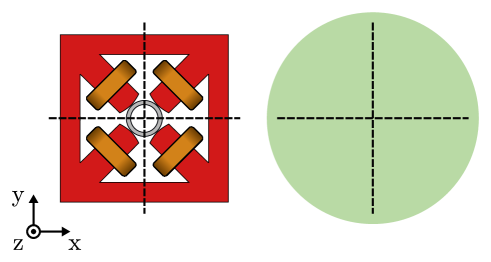
Figure 1: Comparison view of quadrupole in the mass world and the accompanying cylinder used for curvilinear coordinate frame transforms in a parallel world. The curvilinear cylinder has been reduced in size for comparison, but is usually several times bigger to overlap all of the beam line.

For a given global Cartesian position, Geant4 can provide the transform from the volume that point lies within to the world volume and vice-versa irrespective of the depth of the geometry hierarchy. A transform for $N$ levels higher in the geometry hierarchy can also be requested. As the depth of the geometry hierarchy may vary from component to component, this facility cannot be used generally. The local coordinate frame of any given volume is also not necessarily the required curvilinear frame. To provide the correct transforms into the curvilinear frame, BDSIM constructs a separate 3D model (a ‘parallel world’ in Geant4 terminology) with different geometry than that of the beam line. In this parallel world, a simple cylinder of the same length as the accelerator component is placed at the same position as shown in Figure 1.

Any point in the world can then be queried in the parallel world and the transform used from the volume found at that location to the world volume. This will be a transform from the world volume to the local coordinate system of the cylinder whose axis is degenerate with the curvilinear system required. In the case of a component that bends the beam line, many small straight cylinders with angled faces are constructed. This is not exactly the same as the true curvilinear frame, so a dedicated transform is provided.

As already discussed, all Geant4 geometry must have a numerically resolvable gap between adjacent solids and so each parallel world cylinder is placed with a small gap between it and the next one in the beam line. However, if a point is queried in this gap, an incorrect transform will be found. This occurs regularly as the particle enters or exits a volume. The gap between volumes is kept to a minimum to avoid integrating the field over a shorter length. To overcome this problem, a third parallel world is built with bridging cylinders. While searching the curvilinear world for a volume, the world volume itself is found, then the bridging world is subsequently searched. This ensures a continuous coordinate system irrespective of the limits of the geometry system. A quadrupole with curvilinear cylinders and bridging cylinders are shown in Figure 2.

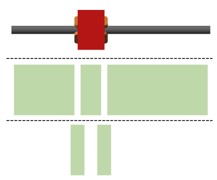
Figure 2: Side view showing the geometry in three different worlds separated by a dashed line. The top-most is the mass world with a beam pipe, quadrupole (red), and beam pipe. The middle world shows three curvilinear cylinders (green) with non-zero gaps between each. These are used for the curvilinear transforms. At the bottom, the third world shows curvilinear bridging sections (green) designed to overlap the above curvilinear cylinders but also have a non-zero gap between them. The bridging cylinder length has been exaggerated for visualisation purposes.

2.3 Fields

Along with the geometry of each beam line element, the required fields are provided. The field strengths are calculated from the rigidity-normalised strength parameters most commonly used to specify accelerator magnets and used in accelerator modelling tools such as MAD–X. For example, in the case of a quadrupole, the normalised strength $k_{1}$ is typically used, which is defined by

$$k_{1}=\frac{1}{B\rho}\frac{\partial B_{y}}{\partial x}$$ (1)

where $B\rho$ is the magnetic rigidity of the particle and $B_{y}$ is the vertical component of the magnetic field. The magnetic rigidity is given by

$$B\rho=\frac{p}{e}$$ (2)

where $p$ is the momentum of the particle and $e$ is the elementary charge. $B\rho$ is calculated for the beam particle the accelerator is designed for and this is used to calculate the magnetic field gradient for a given $k_{1}$. The gradient is evaluated by rearranging Equation 1 and then evaluating it at the coordinates of the particle with

$$B_{x} =x\,\frac{\partial B_{y}}{\partial x},$$ (3)

$$B_{y} =y\,\frac{\partial B_{y}}{\partial x},$$

$$B_{z} =0$$

This is valid close to the axis of the magnet as it neglects any description of the field close to the magnet poles. The pure field like this is used for the vacuum and beam pipe volumes. For the magnet yoke and air in between the poles, a different description is used. Here, a 2D field, invariant along the length of the magnet, is used that is the sum of point current sources located at the point half way between each pole, where the coils would be. The location of each wire is given by

$$\mathbf{c}_{i}=\begin{bmatrix}x\\ y\\ \end{bmatrix}_{i}=\begin{bmatrix}0\\ r_{\mathrm{poletip}}\\ \end{bmatrix}\begin{bmatrix}\cos\theta_{i}&-\sin\theta_{i}\\ \sin\theta_{i}&\cos\theta_{i}\\ \end{bmatrix}$$ (4)

$$\theta_{i}=\left\{\frac{i\,2\pi}{n_{\mathrm{poles}}}\right\}\quad\mathrm{for}\quad i=\{0\ldots n_{\mathrm{poles}}\}$$ (5)

where $r_{\mathrm{poletip}}$ is the radius at the pole tip and $\theta_{i}$ the angle in polar coordinates of the $i^{th}$ wire current source. The magnetic field value $\mathbf{B}$ as a function of position $\mathbf{r}=(x,y)$ is

$$\mathbf{B}(\mathbf{r})=\sum_{i=1}^{n_{\mathrm{poles}}}(-1)^{i}\,\frac{(\mathbf{r}-\mathbf{c}_{i})_{\perp}}{\|\mathbf{r}-\mathbf{c}_{i}\|}$$ (6)

The field is normalised to the pure field at the pole tip radius. This approximate field neglects the permeability of the yoke material, but is sufficient for the purpose as only secondary particles are expected to be transported outside the beam pipe. Should the user wish, they may overlay their own field map for a more accurate description. An example field of this form for a quadrupole is shown in Figure 3.

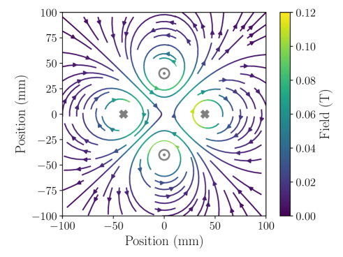
Figure 3: Field for a quadrupole yoke with a pole tip radius of 40 mm as a function of local transverse coordinates. The direction of the current is shown by the grey cross and points at each current source location.

2.4 Physics Processes

Geant4 provides a large library of physics processes. A Geant4 application must instantiate the required particles and then instantiate the required physics process classes and attach them to the applicable particles. Geant4 includes a more convenient general set of ‘physics lists’ that provide commonly used sets of physics processes applicable to many particles for a given application and energy range. These modular lists can be selected by the user in BDSIM and it is left to them to select the most relevant physics processes for the simulation. Using all of the physics processes by default would result in an extremely computationally expensive simulation. Additionally, there may be more than one physics model relevant that the user may wish to choose from. BDSIM provides simple names that map to the most common physics lists constructors in Geant4 as described in Table 1.

Table 1: Examples of name mapping of Geant4 physics lists in BDSIM.

BDSIM Name	Geant4 Class
em	G4EmStandardPhysics
em_livermore	G4EmLivermorePhysics
decay	G4DecayPhysics
ftfp_bert	G4HadronPhysicsFTFP_BERT
ftfp_bert_hp	G4HadronPhysicsFTFP_BERT_HP
hadronic_elasitc	G4HadronElasticPhysics
ion	G4IonPhysics
shielding	G4ShieldingPhysics
stopping	G4StoppingPhysics
synch_rad	G4SynchrotronRadiation

If no processes are selected, only tracking in magnetic fields will be present, i.e. particles will pass unimpeded through matter. Such process-less models are useful for validating particle tracking and beam distributions as well as comparisons to other codes that lack such interactions.

2.5 Run and Event

A BDSIM simulation progresses at two levels; a Run and an Event. An event is the smallest unit of simulation where one initial particle or set of particles is tracked through the model. All information may be collected on an event level basis and all events are entirely independent of each other. A run is a unit of simulation containing $N$ events where the geometry and physics processes do not change.

BDSIM can be run in two ways; interactively with a visualiser; or in batch mode without visualisation. The latter is considerably faster and used for large scale simulation, whereas interactive visualisation is typically used in the preliminary stages to verify the model and typical outcome of an event. In the case of batch mode, BDSIM performs one run with the desired number of events. Interactively, the user may issue the following command on the interactive terminal

⬇

/run/beamOn N

where N is the number of desired events. In this case, BDSIM creates 1 run with N events for each time the command is issued.

Geant4 provides several places in the framework where the developer can insert their own code and gain access to simulation information. BDSIM implements actions at both the beginning and end of each event and run where information is collected, histograms prepared and data written to the output.

2.6 Output

A Geant4 simulation produces no output information by default as the total possible information is unmanageable for storage or analysis. Therefore, it is left to the developer to provide classes that process the information available during the simulation from the Geant4 kernel to create the desired reduced output information. BDSIM uses the Geant4 interfaces and records information from the simulation in two ways.

Firstly, several sensitive detector classes (inheriting G4VSensitiveDetector) are provided and automatically attached to various volumes. These are registered with Geant4 and are provided with access to all particle tracks through the volumes they are attached to. BDSIM includes such a class to record the energy deposition in all volumes in both 3D Cartesian and curvilinear coordinates.

Secondly, BDSIM records trajectory information independently of volumes at an event level. As the full set of trajectories for all particles in an event could reach several gigabytes per event, there are several user options in BDSIM to downselect which trajectories are desired. Each trajectory consists of a series of trajectory points that each contain the spatial coordinates of that point, particle species, total energy and the physics process identification number associated with the last step. Even though a user may filter to select only a certain type of particle, the trajectories are stored in a linked manner so that any individual trajectory point stored can be fully traced back to the primary particle in the event.

In a conventional tracking simulation the coordinates of each particle are updated after passing through each element in the accelerator. Therefore, the most common output is a list of all the particle coordinates after each element. To be able to compare BDSIM to tracking simulations, a similar functionality is provided. BDSIM has a sample command that inserts a ‘sampler’ after either a single specified element or all elements in the beam line. A sampler is a 1 nm thick plane that is 5 m $\times$ 5 m transversely made of vacuum in a parallel world so as not to interfere with the physical interactions. There is no ability to record particles on an arbitrary plane or surface of a volume in Geant4, so a volume must be created and a sensitive detector attached to it. The box is made as thin as possible to minimise artificially increasing the length of the beam line. The sampler plane records any particles passing through it.

Output information is stored in the ROOT data format [23, 24]. This is a well-documented, compressed binary format that is widely used in the high energy physics community. The ROOT data storage facilities are highly suited to storing information on an event by event basis and allow direct serialisation of the developer’s C++ classes as well as provision for data schema evolution. These can be loaded using the compiled software, but the file also contains a complete template of all classes used such that this is not required and the data can always be loaded even if the original software is lost.

Although written in compiled C++, the ROOT framework provides reflection for the classes stored that allows the compiled code to be easily loaded and used interactively in the ROOT interpreter as well as in Python with the exact same functionality allowing users to explore the data interactively with ease.

Aside from raw information, histograms of energy deposition and primary particle impact and loss points are recorded with each event. These can be averaged in analysis to produce the mean energy deposition across all events, but with the correct statistical uncertainty. This treatment is only possible with event by event data storage.

Each data file includes information about the BDSIM options used, random number generator seed states and software identification numbers for BDSIM and its main dependencies to allow any simulation to be strongly recreated. Such information allows reproduction of any simulation immediately or even years later.

2.7 Primary Particle Generation

Generally an event may start with several initial particles (‘primaries’), however, in the case of an accelerator it is more typical to simulate a single particle sampled from a beam distribution.

To begin each event, BDSIM draws randomly a set of coordinates ($x$, $x^{\prime}$, $y$, $y^{\prime}$, $\delta t$, $E$) from a distribution chosen by the user. BDSIM provides 12 possible distributions. The most basic is the ‘reference’ distribution where each particle is the same for each event with a fixed set of coordinates as chosen by the user. These are by default aligned to the axis of the accelerator with no transverse position or momentum. This distribution is used to validate the reference or design trajectory.

A 6D Gaussian distribution is provided where the user may specify the standard deviation $\sigma$ in each dimension as well as the off-diagonal correlation terms in a 6 $\times$ 6 matrix. The Twiss parameterisation common to accelerator beam descriptions is provided, which in turn uses the 6D Gaussian generator.

As one of the purposes of BDSIM is to simulate lost particles interacting with the accelerator, which usually occurs with a low frequency, several distributions are provided that make the simulation more efficient. One such distribution is the ‘halo’ distribution that provides a particle distribution according to the nominal Gaussian beam, but at a large number of $\sigma$.

In all cases, the generator uses a single instance of the pseudo-random number generator from the CLHEP library. The user may specify a starting seed value or one is automatically generated from the computer clock.

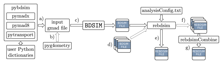
Figure 4: Diagram showing the workflow using the extended tools included with BDSIM. The dashed arrows represent optional steps. From left to right: a) pybdsim is used in combination with other Python packages to prepare an input model including optional input user-provided information in Python dictionaries, b) pyg4ometry can optionally be used to help prepare input geometry, c) BDSIM is used to generate data, d) BDSIM is used many times with multiple seeds on a computer cluster to generate many output files for a study, e) rebdsim is used to analysed one or multiple output files at once using an analysis configuration text file, f) optionally, rebdsim is used one-to-one on output files directly producing one rebdsim file per BDSIM file, in which case g) rebdsimCombine is used to combine these into one result.

2.8 Simulation Control

In each event, particles are tracked until they reach zero kinetic energy or they leave the world (outermost) volume. With high energy primary particles, a very large number of secondaries can be produced and as the particles decrease in energy the number of secondaries can grow, which is known as infrared divergence. Such detail at low energy may not be necessary and may dominate computation time. To avoid this, it is necessary to have some control over the physics processes other than including only those relevant in the physics list.

Geant4 provides the ability to provide tracking cuts in a volume. Here, a minimum energy and maximum time can be specified. If a particle has an energy under or a time greater than these limits, the particle will be removed from tracking. BDSIM provides a method to set limits that will be attached to all volumes and also records the final energy of the particles to conserve energy per event.

In addition to the tracking cuts, Geant4’s primary mechanism is a range cut. A range cut is a distance assigned to a particle species that a secondary of that species would be required to travel. If the secondary would not travel at least that range, the energy deposition is recorded but the secondary particle is not produced. The range is internally converted in Geant4 to a material and particle specific energy cut. This strategy provides the greatest accuracy with the least computation [12]. BDSIM provides an interface to set the range cut for protons, electrons and positrons, photons as well as a default.

Such limits are often necessary as a simulation may not include physics processes that would lead to the natural termination of a particle. For example, synchrotron radiation can produce a very large number of photons making it computationally expensive to track all the secondary particles. The rate scales $\sim\,E^{4}$, so it can dominate when simulating high energy events and therefore is often omitted. This omission however, may lead to low energy particles spiralling in a magnetic field, such as that of a dipole, indefinitely. BDSIM’s numerical integrators have special treatment of spiralling particles, but the user limits provide a convenient method to avoid such scenarios that may lead to long running events with no gain in information.

One further consideration is a circular accelerator. With a circular accelerator and no synchrotron radiation, the particle energy will not decay as the magnetic field does no work. BDSIM therefore provides a circular option to limit the number of turns any primary particle can complete. A 5 m $\times$ 5 m $\times$ 0.1 $\mathrm{\mu}$m cubical volume is inserted between the beginning and end of the lattice that is orientated to make a large transverse plane to the beam. A dynamic set of user limits is attached as well as a special Geant4 sensitive detector class. The sensitive detector class records the number of turns completed by the primary particle and when this has reached the specified number of turns, the user limits are dynamically changed to reject any particle over 0 eV. This makes the box an infinite absorber, stopping any particle that hits it.

2.9 Variance Reduction

With the large number of physics processes included in each physics list as well as the large number of possible outcomes from each interaction, the outcome or process of interest may occur at a low frequency per event. An efficient simulation would simulate the outcome one wishes to characterise for each event, i.e. it is impractical to simulate tens of millions of events to observe only a few occurrences of the desired outcome. When analysing a data set, this effect leads to a large variance of results when in certain areas of parameter space. Biasing is a form of variance reduction where a process or outcome is made artificially more frequent, but recorded with a corresponding statistical weight. Multiplying the simulated frequency by the weight gives the correct physical result but, due to the more frequent occurrence, with a reduced variance. Traditionally, the developer had to write their own C++ wrapper for a given process they wish to study, but recent developments of Geant4 have introduced a more generic biasing interface [25]. Geant4’s generic biasing interface provides both physics based (process cross-section) and non physics based (splitting and killing) such as geometrical importance biasing or importance sampling. An interface to process biasing is provided in BDSIM that allows the user to scale the process cross-section by a given factor for a given particle. The biasing can be applied globally, or to specific vacuum volumes (inside the beam pipe) or the general material (anything outside the beam pipe) of specific beam line elements. For example, this can allow simulation of elastic or inelastic interaction of particles with residual gas molecules in the ‘vacuum’ of the beam pipe.

2.10 Visualisation

At the initial stages of a study, it is crucial to visualise a model to validate its preparation as well as the expected outcome of a typical event. Visualisation is accomplished through an interface to the Geant4 visualisation system that provides a variety of different visualisation programs depending on the software environment.

The default and recommended visualiser is the Geant4 Qt visualiser. This provides a rich interface with an interactive 3D visualisation where the model can be viewed with solid surfaces or as a wire-frame, both with and without perspective. A built in command prompt allows extensive control of the simulation and the visualisation, such as geometry overlap checking and particle track colour schemes.

To visualise an event, all trajectories must be stored. Additionally, the model and all trajectories must be converted to polygon meshes and rendered on screen. Whilst this is handled by the Geant4 visualisation system, this overhead leads to the interactive visualisation system running events approximately an order of magnitude slower than they would without visualisation. The visualisation is crucial in the first stages of a simulation for validation but beyond that it is more desirable to generate as many events as possible in a given time. BDSIM by default will run interactively, but if executed with the --batch option, it will not use the visualiser and complete the simulation with only textual diagnostic and informative output to the terminal. Batch mode is much faster and suitable for simulations that may be run on a computing farm where no graphics systems are available.

2.11 Analysis

Once BDSIM has produced output, this may be analysed using an included analysis suite. This covers the most common basic analysis but also includes an interface for the user to include more complicated analyses.

The main analysis tool is rebdsim (‘ROOT event BDSIM’). This uses a simple text file as input that defines histograms to make from the output structures contained in output files. These can be one to three dimensional histograms made on an event by event basis or as a simple integration across all events. Any histograms stored in the raw output that were produced in BDSIM, such as energy deposition and primary impact location, are combined to produce a mean histogram across all events. The histogram definition in rebdsim specifies which variables in which ‘Tree’ in the output to make the histogram from as well as binning and a ‘selection’. The binning can also be chosen to be logarithmic to cover a large range in values. The selection is an optional weighting that can be a numerical factor, another variable in the data, a Boolean expression based on data variables or a combination of all. This is an interface to that of TTree:Draw in ROOT.

The event level structure in the output is paramount to the analysis for two reasons

1. To calculate the correct statistical uncertainties.

2. To filter independent events on any variable.

To correctly calculate the variance and therefore the statistical uncertainties of any mean histograms, the data must be structured in a per event manner. Conventional tracking programs only simulate one particle per ‘event’ so there is no need to structure data in this way and the uncertainties are trivially calculated. However, with the complex tree of particles and physics processes that can happen per event in a radiation simulation, it is absolutely crucial to structure the data in this way. The default histograms made by rebdsim are made event-by-event and so have the correct statistical uncertainties. The ability to use a selection and filter events based on any variable permits any user analysis to be performed without prior knowledge of the beam line or physical origin of particular information and is highly powerful.

Other attempts at similar simulations typically keep track of very specific information for that application limiting the usefullness of the code. None of the comparable codes already described preserve a per event structure in data and deal only with simple integral histograms and therefore lack the correct treatment of statistical uncertainties.

Using the ‘chain’ feature of ROOT many files can be analysed together behaving as one. Furthermore, a tool rebdsimCombine is provided to combine the output from several instances of rebdsim. For large data sets it would be prohibitive to analyse the whole data set serially, so it is preferable to analyse small chunks in parallel and then combine the resultant histograms. This strategy results in the exact same numerical answer but in a fraction of the time.

The ROOT output format and included analysis tools provide great flexibility in the storage and analysis of simulation data. They also ensure the process is scalable to the very largest data sets dealt with today on the multi-terabyte level.

2.12 Workflow

Apart from the main program, BDSIM, a suite of associated tools is included to facilitate a smooth workflow. These aid in input automatic input preparation and analysis and combination of results as shown in Figure 4.

To aid input preparation, several Python packages are included that aid with different input formats as described in Table 2. There are individual packages for common output formats from accelerator design software such as MAD–X [9], MAD8 [26], and TRANSPORT [27, 28] (pymadx, pymad8, and pytransport respectively). These can be used individually to load, inspect and plot information, but are also tied together by the more general package pybdsim that allows conversion from these formats to a BDSIM model. The conversion includes the ability to include extra information (via user-provided Python dictionaries) in the converted model that may come from other sources, such as aperture or collimator information.

A further tool, pyg4ometry [29, 30], can be used to prepare GDML geometry files for use in BDSIM or any Geant4 simulation. It can also be used to aid in the conversion from other geometry formats. Python scripts can be used to make simple components that can be easily included in a beam line in BDSIM.

Table 2: Included Python packages with BDSIM.

Package	Description
pymadx	Load MAD-X output and create MAD-X models
pymad8	Load MAD8 output and create MAD8 models
pytransport	Parse TRANSPORT input
pybdsim	Convert model using above packages, load and plot raw and analysed BDSIM data

After running BDSIM, the output is a ROOT file with per-event data. This requires analysis as defined by the user to reach a result. Accompanying BDSIM are several other programs that aid with analysis and post-processing of data and are described in Table 3.

Table 3: Included programs other than BDSIM.

Program	Description
rebdsim	Analyse raw BDSIM data files producing a histogram file
rebdsimCombine	Combine multiple histogram files from rebdsim
rebdsimHistoMerge	Combine only pre-made energy deposition histograms from a set of BDSIM data files
rebdsimOrbit	Extract the first hit in each sampler to easily access the primary particle at each sampler
bdsinterpolator	Load BDSIM format field maps, interpolate and export
comparator	Regression testing tool for comparison of data
ptc2bdsim	Convert MAD-X PTC ASCII output to a BDSIM data file for easier comparison with BDSIM data

3 Accelerator Tracking

The Geant4 model constructed by BDSIM provides all the required fields for an accelerator, however, the commonly used numerical integration algorithms provided with Geant4 such as a 4^th order Runge-Kutta integrator will not provide sufficient accuracy for tracking particles through an accelerator. Whilst these numerical integrators are suitable for arbitrary spatially and time varying magnetic and electric fields, the small errors from the numerical integration can accumulate with many successive uses leading to inaccurate results, hence these are rarely used for accelerator tracking. For the specific static magnetic fields of an accelerator, such as a pure dipole or quadrupole field, there are exact solutions that provide more accurate tracking. However, these typically use a coordinate system that follows the accelerator. Algorithms for these tracking routines as well as coordinate system transforms are included with BDSIM and used by default.

The majority of accelerator tracking algorithms use a coordinate system that follows the path of the reference particle (no transverse momentum and exactly the design energy) as opposed to 3D Cartesian coordinates [31]. The Frenet-Serret is such a curvilinear coordinate system as shown in Figure 5.

Figure 5: The curvilinear Frenet-Serret coordinate system ($x$, $y$, $s$) shown following the trajectory of the reference particle. The global Cartesian system is shown (X, Y, Z).

With the Frenet-Serret coordinate system each element’s numerical accuracy is independent from its location and there are no repeated transformations into and out of the system the algorithms are specified in.

Accelerator tracking algorithms can broadly be classed in two categories: thick, and thin. In the thick regime, elements are as long as they are in reality. In the thin regime, a series of instantaneous ‘kicks’, i.e momentum changes, interspersed with drifts are applied to the trajectory. The kicks affect only the transverse momentum and not the position of the particle. As expected, a single kick is not a physically accurate representation of the passage of a particle through a magnetic field, however, the weighted combination of many small kicks in combination with drifts does [32]. The thin regime is often used as it is more computationally performant for a solution that conserves area or volume in phase space. A solution that conserves phase space volume (i.e. symplectic) is required as the tracking algorithms may be applied many times and any small errors will accumulate until the result is no longer physically correct. General symplectic thick solutions exist, but are often more computationally expensive. An accelerator ‘lattice’ is typically first described by a thick lattice that matches the physical accelerator and then potentially converted to a thin lattice.

Geant4 provides a series of numerical integrators that are supplied with spatial coordinates and the field values at that location and are required to predict the particle motion. These must be able to handle a variety of situations that are not encountered in an accelerator tracking program:

• An arbitrary step length.

• Particles with different masses.

• Particles with different charge or that are neutral.

• Backwards travelling particles.

• Particles travelling parallel to a magnetic field.

To introduce accurate and robust accelerator tracking to a Geant4 model, any new integrator must be able to handle these situations. Furthermore, the 3D nature of the model prevents the representation of the accelerator as thin lenses. As Geant4 assumes numerical integration, any new integrator must also estimate a numerical uncertainty associated with the calculation.

BDSIM includes a set of integrators that encapsulate thick tracking algorithms that use the Frenet-Serret coordinate system with special provision for the aforementioned tracking scenarios that may occur in a Geant4 model. These integrators ignore the supplied field from Geant and make use of the normalised strength they are constructed with (e.g. $k_{1}$ for a quadrupole). For dipole and quadrupole fields, an exact analytical solution is possible for the particle motion and numerical integration is not required. For higher order magnets such as sextupoles or octupoles, 2^nd order Euler integrators are provided.

The required coordinate transforms between 3D Cartesian and the Frenet-Serret system make use of the parallel geometry constructed by BDSIM. For scenarios where these algorithms cannot be used, a 4^th order Runge-Kutta integrator is used. It is foreseen that no one set of algorithms may be applicable to all situations, or they may be extended in future, so sets of integrators are used. The user may select from different predefined sets depending on the application. The default set is designed to be both physically accurate and match optical design tools such as MAD–X.

A full mathematical description of all BDSIM integrators is given in the provided documentation [17].

For the most accurate model, the user may choose to use an electromagnetic field map from simulation or measurement. Such field maps can be loaded by BDSIM and overlaid on to both BDSIM and user-provided geometry replacing default fields. The supplied field maps can be easily converted from other formats using the included pybdsim Python utility and can be compressed using gzip. The gzstream library [33] is used to dynamically decompress the text files as they are loaded. BDSIM includes a variety of interpolators to provide the continuous field values in 3D coordinates required by the simulation from the field specified at discrete points in the field map. The user may choose any of the Geant4 numerical integrators ranging from low order Euler to 8^th order Runge-Kutta ones.

This approach allows a user to start with a generic model that will match the design optical description and then further customise with specific field maps.

4 Example

To demonstrate the capabilities and unique features of BDSIM, an example model is provided and illustrated here. The model is of a fictional accelerator that demonstrates many features found in a variety of real accelerators. The model consists of a 4 km racetrack ring with two straight sections that include a low-$\beta$ collision point and a high beta collimation section. Each insertion has a 3-cell half-dipole-strength dispersion suppressor on each side. The most relevant parameters are shown in Table 4. The model and all materials required to prepare it are included with BDSIM as a worked example called ‘model-model’. A schematic layout is shown in Figure 6.

Figure 6: Layout of the example model with race track design including two arc sections, and two insertion regions: ‘IR-collimation’ and ‘IR-lowbeta’. Between each arc and an insertion region there is a dispersion suppressor ‘DS’. The interaction point ‘IP’ is where the beam is focussed to a minimum size.

Table 4: Defining parameters of example model.

Parameter	Value
Particle	proton
Energy	100 GeV
Length	4 km
Dipole bending radius	221.5 m
$\epsilon_{N\,x,y}$	1 mm mrad
Collimators	10
Dipoles	256
Quadrupoles	252
$\beta^{\ast}_{x,y}\*$	2.517 m

The model was created in MAD–X [9] and optical functions as calculated by MAD–X are shown in Figure 7. The low-$\beta$ straight section is designed to create a small symmetric focus of the beam suitable for a collision point with potentially another beam or gas target. The other insertion is designed to expand the beam suitable for collimation or scraping of the beam.

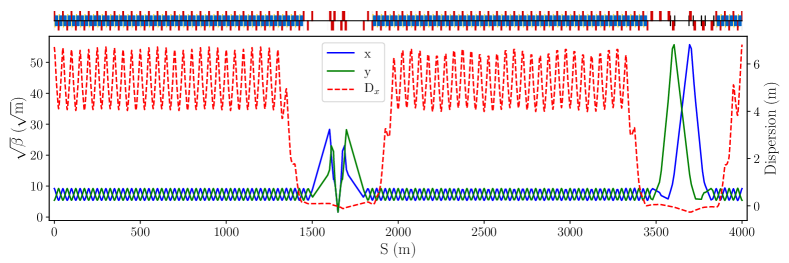
Figure 7: MAD–X linear lattice functions of the example model. The two insertion regions can be seen with reduced horizontal dispersion (red dashed). The first insertion creates a small symmetric beam suitable for collision with another beam or gas target. The second insertion produces a large beam size suitable for collimation. The schematic at the top of the plot depicts each magnet type in the accelerator (blue: dipoles; red: quadrupoles, yellow: sextupoles, black: collimator).

To prepare a BDSIM model an output version is first made from MAD–X using the TWISS command that produces a sequential one-to-one representation of the machine in an ASCII file. This is trivially converted to BDSIM input format GMAD using a provided Python converter pybdsim. Any additional information not specified in this file such as aperture or collimation settings can be included in this conversion with user-supplied Python dictionaries. There is no standard format of auxiliary information about an accelerator so loading this information is left to the user, however Python is a widely used language for which many data loading and processing libraries exist. The automatically converted model includes a Gaussian beam distribution as parameterised by the Twiss parameters from the first element in the sequence and beam information from the header. This fully functional BDSIM model created in minutes acts as a starting point that can then be customised. Figure 8 shows the 3D visualisation of part of the model in BDSIM and Figure 9 shows the magnets from part of a unit cell in the arc.

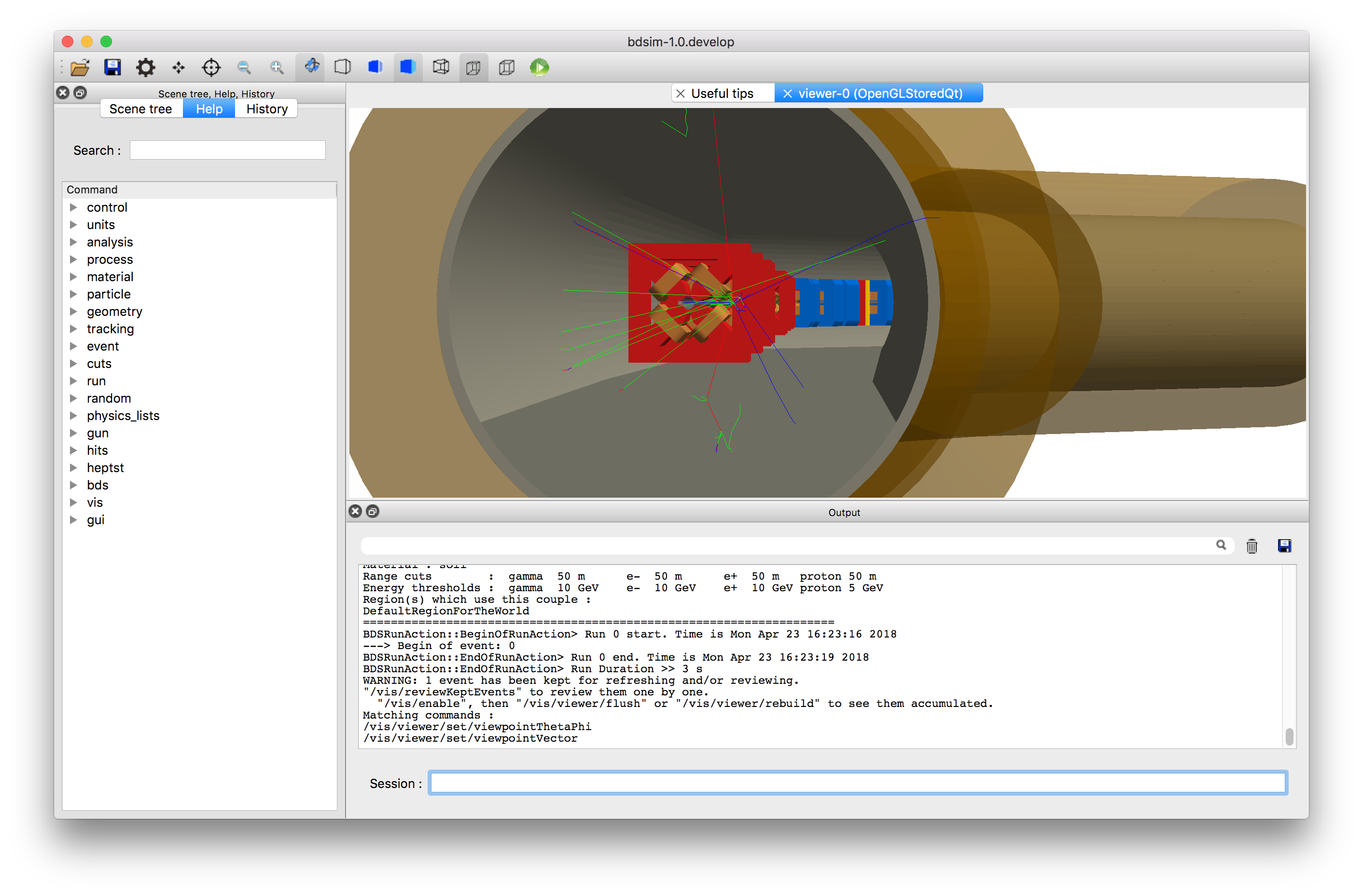
Figure 8: Visualisation of the example model in BDSIM using the Geant4 Qt visualiser. Only part of the machine is visualised showing a single proton impact and secondaries (colour coded by charge). The optional tunnel is automatically built by BDSIM to follow the beam line.

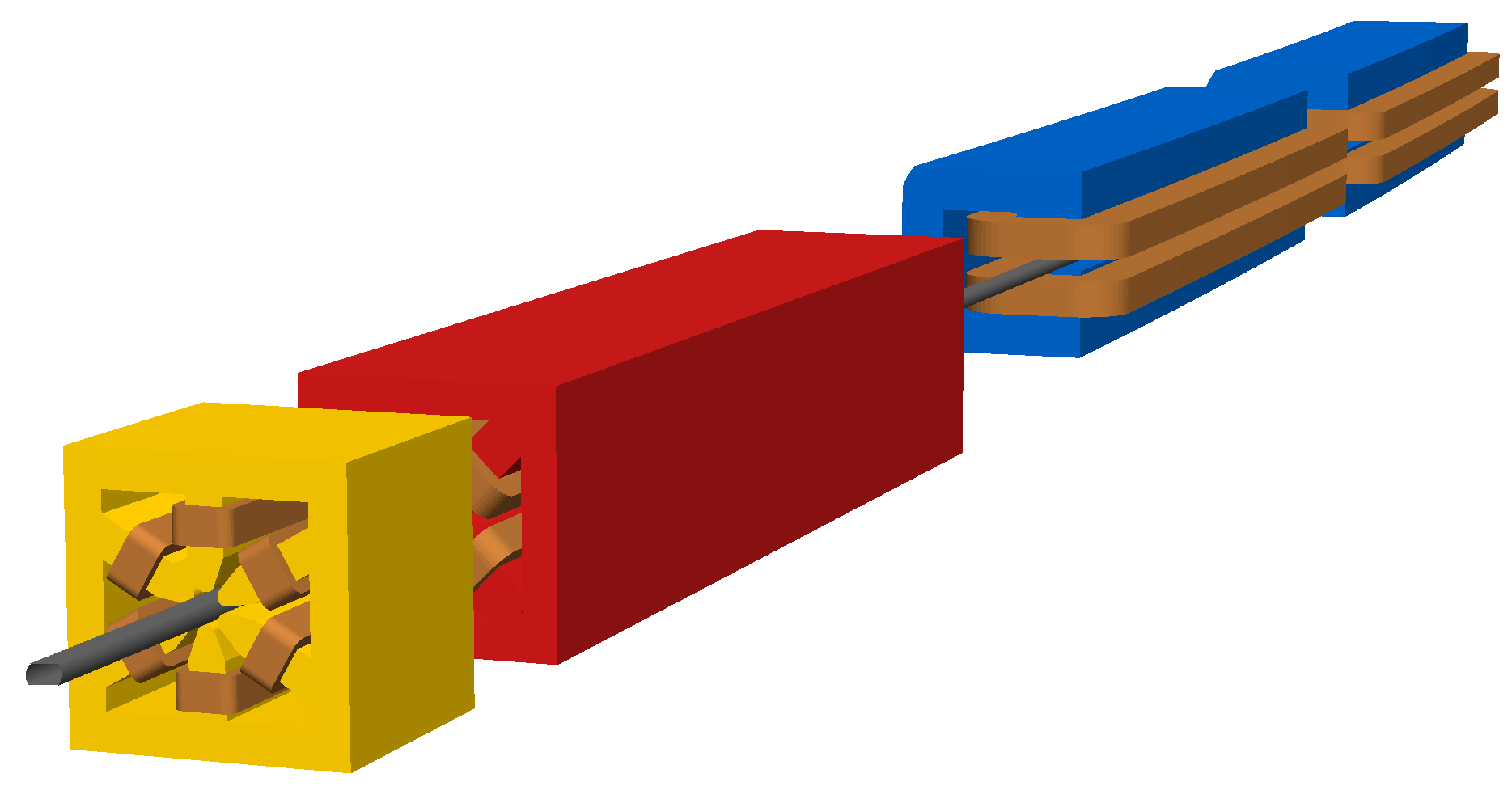
Figure 9: Visualisation of four magnets from the unit cell in the arcs of the example model in BDSIM. From left to right, a sextupole, quadrupole and two sector bends (dipoles) can be seen using the generic geometry provided by BDSIM.

This MAD–X model includes only basic information about the collimators such as their length and perhaps an aperture description, however excludes material definition. The extra required information is provided in an included text file that specifies collimator openings as a specific number of $\sigma$ in the beam distribution at that point as well as material definition. This is used as an example of including extra information into the model conversion and preparation process that could come from an external source. Table 5 illustrates the general settings used in the 3-stage collimation system that has ‘primary’, ‘secondary’ and ‘tertiary’ collimators that are placed at successively greater distances from the beam. Each collimator consists of a rectangular aperture with a narrow opening in one dimension and a more open one in the other that is designed not to impede the beam.

Table 5: Collimator openings in beam $\sigma$. The ‘open’ setting is used for the aperture in the non-collimating plane.

Collimator Type	$\sigma$ opening
primary	6
secondary	7
tertiary	8
open	40

These conceptual settings are used in combination with the MAD–X optical functions to calculate absolute collimator openings in millimetres using an included Python script. These are shown in Table 6.

Table 6: Collimator half openings as calculated from a given beam $\sigma$ and the optical functions at each collimator location. Primary collimators are composed of carbon, secondary collimators copper and tertiary absorbers tungsten that are typical of high energy proton collimation systems with increasing atomic Z.

Name	Material	$\Delta_{x}$ (cm)	$\Delta_{y}$ (cm)
COLPRIMY	C	3.174	2.660
COLSECY	Cu	5.891	3.681
COLPRIMX	C	3.133	6.066
COLSECX	Cu	3.157	3.250
COLTERT	W	1.434	4.437
COLTERT2	W	0.801	0.613
COLTERT3	W	0.523	0.584

The model is prepared using the included pybdsim converter. This allows the extra information for collimators to be included as a Python dictionary that is prepared from the text file. The converter also allows the inclusion of aperture information loaded from a MAD–X TFS file using pybdsim. The classes for aperture loading in pybdsim also permit aperture filtering and substitution. The conversion is shown below where ‘cols’ is a Python dictionary of collimator information by name.

⬇

import pybdsim

import pymadx

ap = pymadx.Data.Aperture(‘ring_aperture.tfs’)

ap = ap.RemoveBelowValue(0.005)

cols = pybdsim.Data.Load(‘collimatorSettings.dat’)

pybdsim.Convert.MadxTfs2Gmad(‘ring.tfs’, ‘bdsim-model’, aperturedict=ap, collimatordict=cols)

The user may use the converted model immediately, edit it to their needs or include the automatically produced GMAD files in their own models. Including the files in a user-written model allows the model to be safely regenerated at any point without losing any user-defined input.

After preparation of a model, the first step is to validate the optical functions of the BDSIM model to ensure correct preparation. To generate optical functions, the automatically provided Gaussian beam distribution according to the Twiss parameters at the start of the machine is used. The beam distribution is sampled after each element in the BDSIM model by including the sampler command in the input gmad:

⬇

sample, all;

To estimate the optical functions, approximately 1–10 thousand particles should be simulated. The model is run with the command:

⬇

bdsim --file=bdsim-model.gmad --outfile=optics1 --batch --ngenerate=1000 --circular

The output ROOT format file ‘optics1.root’ is analysed by an included tool rebdsimOptics that calculates the optical functions as well as the associated statistical uncertainty from the finite population at each sampler is also calculated.

⬇

rebdsimOptics optics1.root opticalfunctions.root

These are calculated by accumulating 1–4^th order power sums and calculating various moments of the distribution. The statistical uncertainty reduces with the number of particles simulated and it is recommended to simulate at least 1000 for a meaningful comparison. rebdsimOptics produces another ROOT format file with the optical function data. The optical functions as calculated from BDSIM can be compared using pybdsim. In this case, we compare against the original MAD–X optical functions the model was prepared from using the following command:

⬇

pybdsim.Compare.MadxVsBDSIM(‘ring.tfs’, ‘opticalfunctions.root’)

This produces a series of plots that compare $\bar{x}$, $\bar{y}$, $\sigma_{x,y}$, $\sigma_{x^{\prime},y^{\prime}}$, $D_{x,x^{\prime}}$, $D_{y,y^{\prime}}$, $\alpha_{x,y}$ and $\beta_{x,y}$, as well as the transmission. An example is shown in Figure 10.

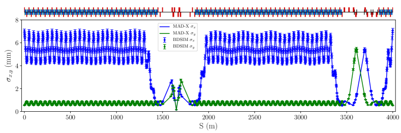
Figure 10: Example machine optical comparison of beam size calculated from MAD–X optical functions, emittance and energy spread with that simulated by BDSIM showing agreement. The beam size in the arc sections is dominated by the dispersion contribution. The schematic at the top of the plot depicts each magnet type in the accelerator and follows the sequence around the ring.

When simulating the optical functions, ideally no particles are lost as this would affect the shape of the beam distribution and the validity of comparing $\sigma$ of the distribution. However, once validated and a physics study is desired, the lack of beam loss makes the simulation very inefficient. For example, to witness an event at 6 $\sigma$, approximately 500 million events would be required on average to be simulated. Therefore, it is logical to select a distribution of primary particles that will collide with the accelerator or exhibit the desired interaction. BDSIM includes a variety of bunch distribution generators for this purpose.

For this example, the intent is to evaluate the performance of the collimation system. Any beam that exists grossly outside the collimator aperture will be immediately lost within one revolution in a circular machine. Similarly, any particle largely inside the collimator aperture will not intercept the collimator. We therefore simulate a thin annulus in phase space that aligns with the edge of the collimator closest to the beam. Such a distribution is provided by the ‘halo’ distribution in BDSIM. This generates particles uniformly in a given phase space volume and accepts or rejects the particle depending on its single particle emittance. Furthermore, spatial limits are provided that allow the phase space to be reduced. An example input distribution is shown in Figure 11.

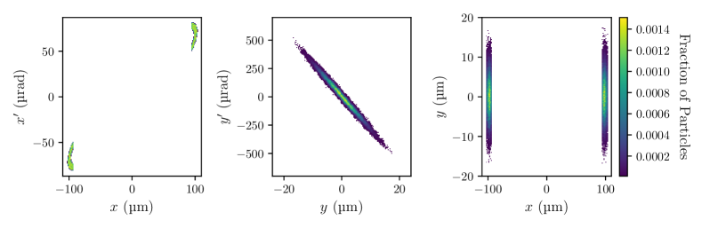
Figure 11: Example phase space distribution for a beam loss simulation using the ‘halo’ distribution based on the Twiss parameters at the entrance to the primary horizontal collimator. The horizontal phase space (left) is designed to intercept a horizontally orientated 2 jaw collimator, whereas the vertical phase space (centre) is the unaltered distribution according to the Twiss parameters. The combination of the two spatially is shown (right). The distribution is exaggerated here with a greater spread in $\sigma$ than is required to make the shape clear. The horizontal phase space is clipped such that only particles with $x>5.7\sigma$ are produced.

In this example, the collimation system is designed to work independently in the horizontal and vertical planes. Therefore, each is simulated independently with the appropriate beam distribution for each dimension. These can later be combined for total beam loss information. Figure 12 shows the combined losses from the simulation of $2\times 10^{5}$ protons with 100 GeV energy in both the horizontal and vertical planes. By default, the user must choose the physics list or sets of processes they require (none were used for the optics validation as none were required). In this case, the Geant4 reference physics list “FTFP_BERT” was used that is a standard high energy physics list provided by Geant4 that BDSIM provides an interface to. This provides a wide variety of physics processes including electromagnetic, hadronic elastic, inelastic and diffractive processes. In BDSIM, it is accessed using the following command:

⬇

option, physicsList="g4FTFP_BERT";

Practically, the simulation was performed on the 500-core Royal Holloway Cluster in 2000 jobs that produced a total 60 GB of ROOT format output. These were analysed individually using rebdsim with the same analysis configuration ASCII file. The resulting 2000 rebdsim histogram files were then combined using the provided rebdsimCombine tool. It should be noted that such large computational resources are not required and one can easily simulate millions of events on a personal computer depending on the size of the model and the physics used.

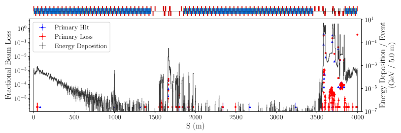
Figure 12: Combined beam loss from a horizontal and vertical halo simulation with $4\times 10^{5}$ primary protons at 100 GeV as a function of distance, S along the axis of the machine. Blue triangles show the point of first contact of primary particles and red circles, their stopping location. The integrated energy deposition is also shown in black recorded by the accelerator geometry. The diagram on top shows the various magnets in order. The beam was started from collimators at $\mathrm{S}=3583$ m (vertical halo) and $\mathrm{S}=3691$ m (horizonal halo). The diagram follows the curvilinear coordinate frame of the machine and is integrated across all turns of all particles, i.e. the diagram wraps around.

Figure 12 shows the proton impact and loss locations. The impact location is determined as the first point where a physics process is invoked along the step of the particle and the loss point is the end of the trajectory of the primary proton. This may be either due to an inelastic collision and subsequent fragmentation, or simply absorption. Additionally, the energy deposition in all material in the accelerator is shown. A clear maximum in losses and energy deposition can be seen in proximity to the collimation section between 3500 m and 4000 m. However, a clear decaying tail of energy deposition is seen throughout the subsequent arc (in the direction of the beam). For the first 1 km of the machine there are very few particle losses but considerable energy deposition. Such energy deposition would not be shown from only tracking primary particles and is a unique feature of BDSIM.

All histograms are made on a ‘per-event’ basis and the histograms shown are the mean of the sampled number of events. The uncertainty for each bin is the standard error on the mean. This allows the statistical sample simulated to be scaled to a realistic rate accurately. Here, one event is one particle simulated. Any realistic rate scaling would take into account the chosen phase space for the input beam distribution that was used for increased simulation efficiency. This per-event analysis is only possible because of the event-by-event storage of the output format and this is crucial to calculate the correct statistical uncertainty associated with each bin in the histogram.

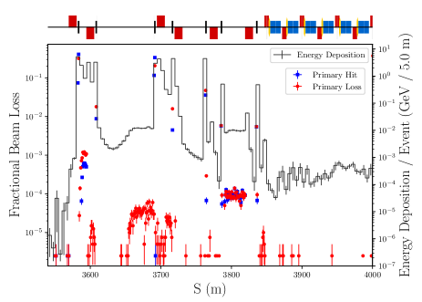
Figure 13: Collimation section detail showing combined beam loss from a horizontal and vertical halo simulation with $4\times 10^{5}$ primary protons at 100 GeV.

Looking at the collimation insertion region in more detail as shown in Figure 13, the pattern of proton impacts and losses can be seen more clearly. The ‘hits’ and ‘losses’ are quite different indicating that primary protons can interact with a collimator and escape. Such information could be used to improve the efficiency of the simplistic collimation section in this model to better absorb the scattered or leaked protons.

The information shown from the simulation is already a powerful guide to the operating radiation produced in the machine. However, further information is easily available that allows an even greater understanding of the machine behaviour. By using the ‘sample’ command on each collimator, the complete distribution of particles after each element can be recorded.

Figure 14 shows the energy spectrum of particles recorded in a sampler placed after the primary horizontal collimator for the horizontal halo simulation. For each particle species a separate histogram was prepared with rebdsim by defining a ‘selection’ that acts as a filter. Here, the integer particle ID from the Monte Carlo Numbering scheme [34] was matched. The spectra show significant fluxes of various high energy particles leaving the primary collimator and in particular a much broader spectrum of primary protons than were originally in the beam. These are of particular interest as they may travel some distance before being lost in a position that would not be immediately associated with the collimator in question.

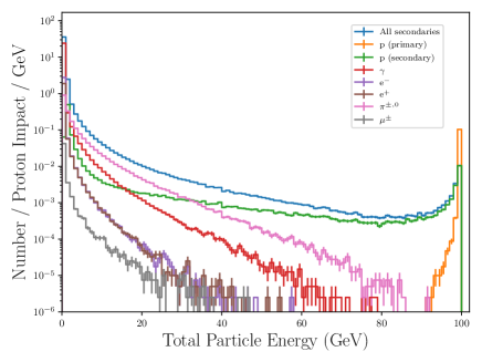
Figure 14: Particle energy spectrum of all particles recorded after the primary horizontal collimator. The data is integrated for all 100 revolutions of the primary beam in the simulation.

Furthermore, for the purpose of damage and activation it is useful to look at the neutron distribution as an example. Shown in Figure 15 is the 2D distribution of neutrons weighted by their total energy after the secondary horizontal collimator from the horizontal halo simulation only. Here, a clear shadow of the collimator can be seen. The rebdsim input syntax is shown below to highlight the simplicity of making per-particle-species rate normalised histograms from simulation data without the need for a complicated analysis.

⬇

Histogram2D

Event.

COLPRIMXEWFluxProtSecZoom

{100,100}

{-0.5:0.5,-0.5:0.5}

COLPRIMX.y:COLPRIMX.x

COLPRIMX.energy*(COLPRIMX.partID==2112&&COLPRIMX.parentID>0)

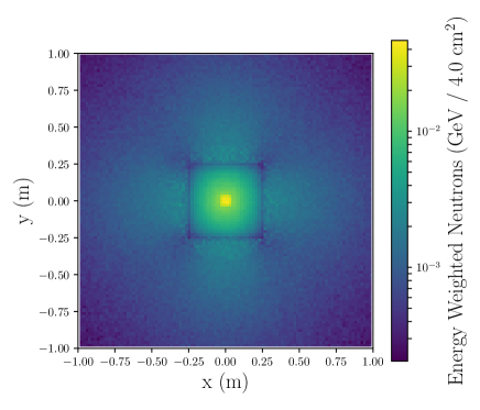
Figure 15: The energy-weighted neutron flux after the secondary horizontal collimator per proton impact on the primary collimator. Although the collimators have an asymmetric aperture, their outer shape is a square. Here the shadow of the square 0.5 m wide collimators can clearly be seen.

For circular models, the losses as a function of turn number are important. BDSIM records the turn number associated with all data in the output for circular models permitting turn-by-turn analysis. Figure 16 shows the surviving fraction of the simulated halo beam after each turn. The periodic steps are due to the tune of the circular machine and the figure illustrates the different performance of the collimation system in each plane. Should it be desired, the data presented in Figure 14 and Figure 15 can easily be filtered by turn number to show the radiation on a particular turn or range of turns that may correspond to a sharp increase of losses.

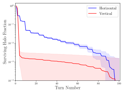
Figure 16: Fraction of primary halo protons surviving per turn completed in the ring for both the horizontal and vertical halo simulations. The coloured band represents the statistical uncertainty from the simulation.

5 Validation

5.1 Tracking Validation

Tracking accuracy is crucial for physics studies to correctly describe the machines being simulated. Imprecise tracking in any single component would result in incorrect subsequent tracking in the machine. This is particularly relevant to circular machines that would suffer immensely from cumulative errors due to the high number of components and repeated passage of particles.

Individual components in BDSIM as well as the optical functions of many large current accelerators have been tested extensively in BDSIM over many years and optical agreement is expected out-of-the-box. To demonstrate tracking validation, the most obvious route is to compare with existing particle tracking software. However, care must be taken to make such a comparison correctly and accurately. In particular, most accelerator codes output data in ASCII format and the transfer of numerical coordinates via such files can lead to truncation and severe loss of precision. Furthermore, many tracking programs operate with an assumed range of validity, such as the paraxial approximation, or can be used with different integrators. MAD–X PTC for example, can be used with the expanded or exact Hamiltonian, which can lead to vastly different results. Several tracking programs have implicit assumptions such as the primary particle being assumed to be fully relativistic. Particle tracking codes often allow the user to choose between computational performance and increased physical accuracy depending on their needs. With this knowledge in mind, any comparisons between codes must be carefully performed with knowledge and understanding of the limitations of particular software.

The validation of BDSIM tracking has been performed and ensures that:

1. The output of the implementation of an individual integrator matches that of the mathematical description as documented in the manual.

2. The automatic preparation and conversion of a model is correct and accounts for the often inconsistent output of the supported optical descriptions.

3. A converted model reproduces the expected optical functions throughout a lattice.

In addition, to the caveats of using other tracking software, we must consider also how information is recorded in BDSIM. In particle tracking software, an algorithm is applied to a set of coordinates representing the traversal through an accelerator component. The coordinates reported after this single traversal represent the particle precisely at the end of the element. However, in BDSIM, we make a 3D model where no 2D shapes can exist. It is not possible through the interfaces in Geant4 to record particles at only one surface of a multi-faceted solid (e.g. one face of a cube). We must also avoid coplanar faces or geometrical overlaps with a numerically resolvable gap in-between each element for robust geometry navigation and tracking. In BDSIM, the particle coordinates are recorded on the one step taken through the 1 nm thin sampler, which is placed after the element with a 1 nm gap between each surface. This difference in distance may introduce a very small difference in coordinates and agreement is expected only to this degree. The distance between surfaces in BDSIM was carefully chosen and the spacing of faces around the end of each element in both the mass world and the several parallel worlds chosen so as to avoid coplanar faces between worlds wherein Geant4 would incorrectly navigate through the geometry.

Particle to particle comparisons show residuals at the level of $10^{-9}$ in both position (m) and transverse (normalised) momentum for particles in the paraxial approximation for the most common design of magnets (length and strength) found in a large variety of accelerators. The comparison was made by specially compiling BDSIM with double precision floating point output and increasing the precision of the output from MAD–X PTC.

Optical comparisons for a variety of accelerators including the LHC, the Accelerator Test Facility 2 (ATF2) at KEK, Japan, the Diamond Light Source (DLS), UK, show excellent agreement with both MAD–X PTC and the optical functions from MAD–X. The LHC demonstrates accuracy through a large number of components. The ATF2 demonstrates correct transport through a highly non-linear lattice where pole face rotations and dipole fringe fields are important. The ATF2 magnifies a beam before creating a nanometre-level focus, so any small deviations are readily observable. The DLS demonstrates a machine whose performance is highly dependent on chromatic and dispersive effects. When testing large lattices it is common to witness a deviation in the mean in several parameters. This is due to the finite sample of particles used, where the initial sample-based mean is non-zero. Such a non-zero offset is then witnessed as it propagates. BDSIM includes an advanced option where the sample deviation may be subtracted by pre-generating the full distribution and calculating the sample mean from it. This is only valid for large sample sizes and is used for developer optical comparisons.

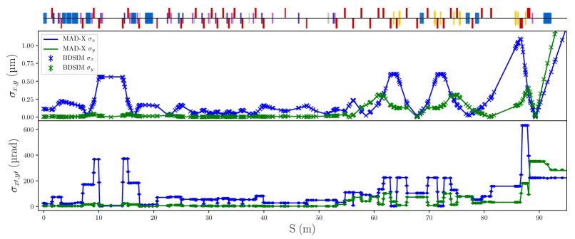
Figure 17: Comparison of beam size (top) and angular size (bottom) between tracking in BDSIM (points) and the MAD–X model (solid line) throughout the Accelerator Test Facility 2 (ATF2) extraction line at KEK, Japan. After extraction from a damping ring, the beam progresses left to right along a single pass extraction line. The comparison shows excellent agreement throughout as the beam size is strongly manipulated. The effect of dipole pole face rotations is not visible directly but is evident in the agreement that would be coarsely wrong if this minuscule effect was omitted.

Although the tracking routines provided are demonstrably accurate, as already mentioned, the 3D model must include a small numerically resolvable gap between each volume. For long term tracking in circular accelerators, such geometrical effects accrue and can result in inaccurate tracking. However, the purpose of BDSIM is not to perform long-term tracking studies, but to simulate losses and subsequent radiation. As shown in Section 4, a collimation simulation typically starts only with particles that impact a collimator. For a typical LHC collimation study, up to 200 turns of tracking are permitted [8]. For a particle at approximately one sigma of the nominal distribution, an offset of 3 $\mathrm{\mu}$m is accrued after 200 turns which is acceptable.

As tracking in a BDSIM model is ultimately performed in Cartesian coordinates, BDSIM cannot be used for arbitrarily large circular machines. This is because the numbers for each coordinate are stored as double precision floating point numbers. When a particle makes an excursion to the furtherst part of the ring where there maybe an offset of tens of kilometres, the $\sim$15 significant figures will lead to a lack of precision in curvilinear coordinates. This is not foreseen as a problem as the largest existing machine is the LHC, where the tracking has been shown to be acceptable for radiation simulations.

A common concern in particle tracking software is whether the tracking is symplectic. This is equivalent to precisely conserving energy and phase space volume after both a single and multiple applications of a transfer map or algorithm. The integrators of the linear elements in BDSIM are thick lens solutions and are symplectic. The higher order integrators are low-order semi-implicit Euler integrators that are symplectic. These conserve energy but cannot be used accurately for large step sizes and be physically accurate. In practice, the numerical integration error is estimated and returned to Geant4 that limits the step size in strongly varying magnetic fields. In validation testing, it was found that the accrued geometrical errors dominate in larger circular models. In linear models, the tracking is sufficiently accurate and symplecticity is not of concern.

In the case of circular machines, it is possible to use a one-turn-map with BDSIM. This is an externally provided transfer map representing a single turn of the circular machine that can be used to correct the particle coordinates on each turn. If the particle completes a turn of the circular machine without any physics process being invoked, the coordinates after the turn are calculated independently for that turn using the map and the particle coordinates updated. This approach allows a maximum error of approximately $1\,\mathrm{\mu}$m to be achieved for up to 10,000 turns of the LHC using a 14th order map calculated by MAD–X PTC. It should be noted however, that if the lattice contains non-linear elements, the map will typically be non-symplectic. However, with a high order map, it would take a high number of turns outside the applicability of BDSIM to reach this limitation.

For the purpose of simulating accelerators smaller than the LHC and linear or single pass sections, the tracking is highly accurate.

5.2 Quality Assurance

To be used in a predictive capacity, aside from validation there must be assurance that any changes or modifications to the software do not affect any known outcome. Any new additions must also be demonstrated to work reliably with a variety of input. BDSIM uses two main types of tests to ensure the quality and stability of the software, namely unit and regression tests.

Unit tests are minimal input examples that exploit a particular feature. Running such an example in BDSIM forces use of the feature in the BDSIM code and tests it executes without problem. For every test of correct input there are matching tests of incorrect input that BDSIM should reject. The condition for the test to pass in this case is that BDSIM should exit. At the time of writing there are 689 unit tests that cover 87.61% of the C++ code in BDSIM. The parts not covered are identified as parts that are for external interfaces and are tested elsewhere or for interactive visualisation that cannot be tested automatically, but are however covered by regular use. The tests are defined in CMake [35] as part of the build system throughout the examples directory and are run with CTest, which is part of CMake. Every example also forms a unit test. The majority of tests are run single-threaded within 1hr and are automatically run at the Royal Holloway Faraday Cluster up to every hour if the code is updated in the public-facing git repository. The results are reported to a CDash website hosted at Royal Holloway, where code coverage and test results and output can be inspected. Developers are automatically notified of newly failing tests due to commits they have made. Several builds for Scientific Linux 6 and 7 and Ubuntu operating systems are made. In addition, separate builds for Geant 4.10.1 through to 4.10.5 are made and all tests running for each. This variety gives very good coverage of operating systems and environments that are expected to be used for BDSIM.

In addition to unit tests, regression test are used. Unit tests ensure that there is no syntactic or logical problem with the code, but not that it achieves the correct result. Regression tests are used to compare the output of a fresh simulation with a manually validated result. To make the comparison, a special tool, the comparator, is included with BDSIM. This is capable of dynamically inspecting all the data structures found in a BDSIM output file and comparing them. In the case of coordinates at a sampler plane, individual entries can be compared within the numerical precision of the output. In these cases, tests are conducted with the same random number generator seed, so the output should be identical. In the case where two histograms are compared, the contents can be compared statistically using the Student’s T-Test.

Several reference output files are created for large accelerators such as the ATF2, DLS and the LHC included in the examples. These contain a large variety of elements with a large variety of settings, so provide a high level of coverage over tracking algorithms. Any change in these will be shown by the single-turn or pass coordinates being different. The developers can then investigate to identify the precise cause of the discrepancy. Aside from complete lattices, many references files are included for key features of BDSIM as well as several examples that use a combination of many options.

Aside from developer-side testing, BDSIM uses a publicly visible software repository using the git software versioning software [36]. The BDSIM website, (http://bitbucket.org/jairhul/bdsim), also hosts a public issue tracker where anyone can report an issue and is regularly updated by the developers. The use of the git software versioning system in a public repository allows users to review and understand both how BDSIM works as well as possibly contribute. The authors have found the open-source nature to be invaluable in fostering a community that understands and contributes to the code.

Usage of the code is documented in an included manual prepared using the commonly used Sphinx documentation system [37]. This allows export of the manual as both an HTML website and LaTeX document that is rendered as a PDF, ensuring both are consistent. The classes and structure of the code is documented using Doxygen [38] that parses comments in the source files. The code is fully documented using this system and the output Doxygen website is publicly hosted.

6 Conclusions

BDSIM is an open source C++ code that makes use of widely used and current high energy physics software to provide a mixed 3D and accelerator tracking simulation suitable for predicting the radiation in and around an accelerator.

It provides a unique capability to accurately simulate radiation transport in an accelerator environment. It significantly simplifies the construction of a 3D Geant4 model by providing a library of generic but scalable accelerator components as well as the appropriate fields and numerical integrators for the most accurate particle tracking. Additional thin elements such as multipoles and magnet fringe elements ensure accurate magnetic tracking that matches the most commonly used accelerator tracking codes. Furthermore, the ability to track all particles through the accelerator with arbitrary step sizes is unique and allows prediction of the radiation transmitted through and around an accelerator. The data format and provided analysis tools are built on ROOT, software used commonly in particle physics, that is highly scalable and suitable for long term data storage and very large data quantities.

The included Python utilities allow preparation of models in minutes that would normally take several weeks to prepare manually and are easily extendable with further user input and customisation. As BDSIM as well as all of its dependencies are open source, the program is highly transparent to the user with complete and regularly updated documentation. Furthermore, the software can be easily extended with user’s C++ code.

BDSIM has been engineered to be applicable to both the lowest and highest energy accelerators in use today. It provides a unique ability to perform a mixed accelerator and radiation transport simulation as well as remove many obstacles for developing a beam line model. The software was written in a way to support the widest set of simulations and beam lines.

7 Acknowledgements

The development of BDSIM has received funding from the John Adams Institute at Royal Holloway. This work was supported by Science and Technology Research council grant “The John Adams Institute for Accelerator Science” ST/P00203X/1 and Impact Acceleration Account. It was also supported in part by EU FP7 EuCARD-2, Grant Agreement 312453 (WP13, ANAC2) and STFC, United Kingdom. Thank you to J. Albrecht, S. E. Alden, D. Brewer, A. Cooper, W. Parker, J. Van Oers, M. Porter and S. Williams for their contributions and testing.

References

- [1] CERN Report ICFA Panel on Spin-Off from Particle Physics.
- [2] J. Arthur, et al., Linac Coherent Light Source (LCLS) Conceptual Design Report, Slac-R-593 (April) (2002) 554. doi:10.2172/1029479.
- [3] K. Balewski, W. Brefeld, W. Decking, H. Franz, R. Rohlsberger, E. Weckert, PETRA III: A low emittance synchrotron radiation source. Technical design report (2004).
-
[4]
Detailed
design report on the MAX IV facility (2010) [cited December 2019].
URL https://www.maxiv.lu.se/accelerators-beamlines/accelerators/accelerator-documentation/max-iv-ddr/ -
[5]
O. S. Brüning, P. Collier, P. Lebrun, S. Myers, R. Ostojic, J. Poole,
P. Proudlock, LHC Design Report,
CERN Yellow Reports: Monographs, CERN, Geneva, 2004.
doi:10.5170/CERN-2004-003-V-1.
URL https://cds.cern.ch/record/782076 -
[6]
P. Lebrun,
Cryogenics for
high-energy particle accelerators: highlights from the first fifty years,
IOP Conference Series: Materials Science and Engineering 171 (2017) 012001.
doi:10.1088/1757-899x/171/1/012001.
URL https://doi.org/10.1088%2F1757-899x%2F171%2F1%2F012001 - [7] G. Valentino, R. Aßmann, R. Bruce, F. Burkart, V. Previtali, S. Redaelli, B. Salvachua, G. Stancari, A. Valishev, Beam diffusion measurements using collimator scans in the LHC, Phys. Rev. ST Accel. Beams 16 (2013) 021003. doi:10.1103/PhysRevSTAB.16.021003.
- [8] R. Bruce, R. W. Assmann, V. Boccone, C. Bracco, M. Brugger, M. Cauchi, F. Cerutti, D. Deboy, A. Ferrari, L. Lari, A. Marsili, A. Mereghetti, D. Mirarchi, E. Quaranta, S. Redaelli, G. Robert-Demolaize, A. Rossi, B. Salvachua, E. Skordis, C. Tambasco, G. Valentino, T. Weiler, V. Vlachoudis, D. Wollmann, Simulations and measurements of beam loss patterns at the cern large hadron collider, Phys. Rev. ST Accel. Beams 17 (2014) 081004. doi:10.1103/PhysRevSTAB.17.081004.
-
[9]
Methodical Accelerator Design X
(2019) [cited December 2019].
URL http://madx.web.cern.ch/madx - [10] F. Schmidt, E. Forest, E. McIntosh, Introduction to the polymorphic tracking code: Fibre bundles, polymorphic taylor types and exact tracking (2002).
- [11] F. Schmidt, SIXTRACK version 1.2: Single particle tracking code treating transverse motion with synchrotron oscillations in a symplectic manner: User’s reference manual (1994).
- [12] S. Agostinelli, et al., GEANT4: A simulation toolkit, Nucl. Instrum. Meth. A506 (2003) 250–303. doi:10.1016/S0168-9002(03)01368-8.
- [13] G. Battistoni, T. Boehlen, F. Cerutti, P. W. Chin, L. S. Esposito, A. Fassò, A. Ferrari, A. Lechner, A. Empl, A. Mairani, A. Mereghetti, P. G. Ortega, J. Ranft, S. Roesler, P. R. Sala, V. Vlachoudis, G. Smirnov, Overview of the {FLUKA} code, Annals of Nuclear Energy 82 (2015) 10 – 18. doi:https://doi.org/10.1016/j.anucene.2014.11.007.
- [14] K. L. Brown, F. C. Iselin, Decay TURTLE (Trace Unlimited Rays Through Lumped Elements): A Computer Program for Simulating Charged Particle Beam Transport Systems, Including Decay Calculations, CERN-74-02 (1974).
- [15] C. Kost, P. A. Reeve, A Monte Carlo Beam Transport Program: REVMOC, in: Computing in Accelerator Design and Operation. Proceedings, EuroPhysics Conference, Berlin, Germany, 1983.
-
[16]
BDSIM - Beam Delivery
Simulation (2019) [cited December 2019].
URL http://www.pp.rhul.ac.uk/bdsim/ -
[17]
BDSIM manual (2019) [cited
December 2019].
URL http://www.pp.rhul.ac.uk/bdsim/manual - [18] I. Agapov, G. A. Blair, S. Malton, L. Deacon, BDSIM: A particle tracking code for accelerator beam-line simulations including particle-matter interactions, Nucl. Instrum. Meth. A606 (2009) 708–712. doi:10.1016/j.nima.2009.04.040.
-
[19]
M. Inc., G4beamline
(2019) [cited December 2019].
URL http://www.muonsinternal.com/muons3/G4beamline -
[20]
Flex website (2019) [cited December
2019].
URL https://github.com/westes/flex -
[21]
GNU bison (2019) [cited December
2019].
URL https://www.gnu.org/software/bison/ - [22] R. Chytracek, J. McCormick, W. Pokorski, G. Santin, Geometry description markup language for physics simulation and analysis applications., IEEE Trans. Nucl. Sci. 53 (2006) 2892. doi:10.1109/TNS.2006.881062.
- [23] R. Brun, F. Rademakers, ROOT: An object oriented data analysis framework, Nucl. Instrum. Meth. A389 (1997) 81–86. doi:10.1016/S0168-9002(97)00048-X.
- [24] I. Antcheva, M. Ballintijn, B. Bellenot, M. Biskup, R. Brun, N. Buncic, P. Canal, D. Casadei, O. Couet, V. Fine, L. Franco, G. Ganis, A. Gheata, D. G. Maline, M. Goto, J. Iwaszkiewicz, A. Kreshuk, D. M. Segura, R. Maunder, L. Moneta, A. Naumann, E. Offermann, V. Onuchin, S. Panacek, F. Rademakers, P. Russo, M. Tadel, Root — a C++ framework for petabyte data storage, statistical analysis and visualization, Computer Physics Communications 180 (12) (2009) 2499 – 2512. doi:https://doi.org/10.1016/j.cpc.2009.08.005.
- [25] J. Allison, et al., Recent developments in GEANT4, Nuclear Instruments and Methods in Physics Research Section A: Accelerators, Spectrometers, Detectors and Associated Equipment 835 (Supplement C) (2016) 186 – 225. doi:https://doi.org/10.1016/j.nima.2016.06.125.
-
[26]
H. Grote, F. C. Iselin, The MAD
program (methodical accelerator design): version 8.10 ; user’s reference
manual; 3rd ed., CERN, Geneva, 1993.
URL https://cds.cern.ch/record/248416 -
[27]
K. L. Brown, D. C. Carey, F. C. Iselin, F. Rothacker,
TRANSPORT: a computer program for
designing charged-particle beam-transport systems, CERN Yellow Reports:
Monographs, CERN, Geneva, 1980, also publ. as SLAC and FERMILAB.
doi:10.5170/CERN-1980-004.
URL http://cds.cern.ch/record/133647 - [28] U. Rohrer, PSI Graphic Transport Framework based on a CERN-SLAC-FERMILAB version by k.l. brown et al.
-
[29]
pyg4ometry (2019) [cited
December 2019].
URL https://bitbucket.org/jairhul/pyg4ometry -
[30]
pyg4ometry manual (2019)
[cited December 2019].
URL http://www.pp.rhul.ac.uk/bdsim/pyg4ometry - [31] W. H., Particle Accelerator Physics, 3rd Edition, Springer, 2007. doi:10.1007/978-3-540-49045-6.
- [32] L. Schachinger, R. Talman, Teapot: A Thin Element Accelerator Program for Optics and Tracking, Part. Accel. 22 (1987) 35.
-
[33]
D. Bandyopadhyay, L. Kettner,
Gzstream library
(2019) [cited December 2019].
URL https://www.cs.unc.edu/Research/compgeom/gzstream/ - [34] M. Tanabashi, et al., Particle data group, Phys. Rev. D 98 (2018) 030001.
-
[35]
CMake (2019) [cited December 2019].
URL https://cmake.org -
[36]
Git (2019) [cited December 2019].
URL https://git-scm.com -
[37]
Sphinx (2019) [cited December
2019].
URL https://www.sphinx-doc.org/en/master/ -
[38]
Doxygen documentation system (2019) [cited
December 2019].
URL http://www.doxygen.nl