Full-Duplex Energy-Harvesting Enabled Relay Networks in Generalized Fading Channels

Abstract

This paper analyzes the performance of a full-duplex decode-and-forward relaying network over the generalized $\kappa$-$\mu$ fading channel. The relay is energy-constrained and relies entirely on harvesting the power signal transmitted by the source based on the time-switching relaying protocol. A unified analytical expression for the ergodic outage probability is derived for the system under consideration. This is then used to derive closed-form analytical expressions for three special cases of the $\kappa$-$\mu$ fading model, namely, Nakagami-$m$, Rice and Rayleigh. Monte Carlo simulations are provided throughout to verify the correctness of our analysis.

I Introduction

Simultaneous wireless information and power transfer (SWIPT) in full-duplex (FD) relaying networks has recently attracted a great deal of research attention. For instance, the authors in [1] considered a dual-hop FD SWIPT network with both amplify-and-forward (AF) and decode-and-forward (DF) relaying protocols equipped with a single antenna. Several analytical expressions of the achievable throughput were derived. Instead of the single-antenna relay, the authors in [2] extended the work in [1] to include multiple-input multiple-output (MIMO) FD relaying. Unlike [1] and [2], which focused on Rayleigh fading channels, the work in [3] analyzed the performance of a FD SWIPT system in indoor environments characterized by log-normal fading. The study in [4] considered the outage probability of FD SWIPT networks over $\alpha-\mu$ fading channels. Furthermore, the authors in [5] studied physical layer security in FD two-way relaying for SWIPT. More specifically, AF relaying with multiple antennas and zero-forcing was deployed in this work. Other studies exploiting jamming signals for EH have recently appeared in [6, 7].

None of the aforementioned works considered FD energy-harvesting (EH)-enabled relay networks over generalized fading channels. In contrast, and motivated by this lack of analytical analysis, we present in this letter a thorough performance evaluation of FD EH-enabled relay networks over the generalized $\kappa$-$\mu$ fading channel. Specifically, DF and time-switching relaying (TSR) protocols are deployed at the relay. The motivations of our work come from the following two factors. Firstly, the $\kappa$-$\mu$ model is a small-scale fading model and is able to characterize the scattering cluster in homogeneous communication environments including Rice $\left(\kappa=k,\,\mu=1\right)$, Nagakami-$m$ $\left(\kappa\rightarrow 0,\,\mu=m\right)$ and Rayleigh $\left(\kappa\rightarrow 0,\,\mu=1\right)$ [8, 9, 10]. Secondly, FD communication allows devices to operate on the same frequency, which potentially doubles the spectral efficiency, and, because of this, FD has become a viable option for next generation wireless communication networks. Thus, the network studied herein is meaningful and valuable for consideration.

The main contribution of this letter resides in deriving a novel unified analytical expression for the ergodic outage probability of the proposed system over the generalized $\kappa$-$\mu$ fading channel. In addition, closed-form expressions for the aforementioned special cases of the $\kappa$-$\mu$ fading scenario are presented. The derived expressions were used to investigate the impact of several system and fading parameters on the performance. Results show that the performance can be enhanced considerably as the fading parameters $\kappa$ and $\mu$ are increased. It is also shown that as the loop-back interference, associated with FD relaying, increases the outage probability performance deteriorates drastically.

II System Model

The considered system model consists of a source (S), a relay (R) and a destination (D). The end nodes are equipped with a single antenna whereas R, based on DF, has two antennas operating in FD mode. It is assumed that there is no direct link between the end nodes due to severe shadowing and path-loss effect [1, 2, 3, 5]; hence, all communication is accomplished over two phases. The S-to-R, R-to-D and loop-back interference channel coefficients, denoted as $h_{1}$, $h_{2}$ and $h_{3}$, are assumed to be independent but not necessarily identical following the $\kappa$-$\mu$ distribution with a probability density function (PDF)

$$f_{Z_{i}}\left(z\right)=\Upsilon_{i}\,z^{\frac{\mu_{i}-1}{2}}\,\textrm{exp}\left(-\frac{\phi_{i}\,z}{\Omega_{i}}\right)I_{\mu_{i}-1}\left(2\mu_{i}\sqrt{\frac{\phi_{i}\,z}{\Omega_{i}}}\right),$$ (1)

where $i\in\left\{1,2,3\right\}$, $Z_{i}=h_{i}^{2},$ $\Omega_{i}=\mathbb{E}\left[Z_{i}\right]$, $\phi_{i}=\mu_{i}\left(1+\kappa_{i}\right),$ $\Upsilon_{i}=\frac{\mu_{i}\left(1+\kappa_{i}\right)^{\frac{\mu_{i}+1}{2}}}{\textrm{exp}\left(\mu_{i}\kappa_{i}\right)\kappa_{i}^{\frac{\mu_{i}-1}{2}}\Omega_{i}^{\frac{\mu_{i}+1}{2}}}$, $I_{v}\left[\cdot\right]$ is the modified Bessel function of the first kind with arbitrary order $v$ [11, Eq. 9.6.20], $\mu_{i}$ represents the number of the multipath clusters and $\kappa_{i}>0$ denotes the ratio between the total powers of the domain components and the scattered waves. The path-loss exponents for the S-to-R and R-to-D links are denoted by $\xi_{1}$ and $\xi_{2}$, respectively. It is assumed that perfect channel state information (CSI) is available at all receiving nodes. R has no power supply and operates by harvesting the RF signal coming from S. The energy used for information processing at R is negligible and hence all the harvested energy will be utilized to forward the source information.

As mentioned earlier, the TSR protocol is used for EH at R, in which the time frame $T$ is divided into two consecutive time slots: $\alpha T$ and $\left(1-\alpha\right)T$, which are used for EH and S-to-R / R-to-D information transmissions, respectively; where $0\leq\alpha\leq 1$ is the EH time factor.

For the sake of brevity, we omit the mathematical modeling of the received signals at R and D and present only the corresponding signal-to-noise ratios (SNRs). Readers may refer to [1, 3] for more details. The SNRs at R and D nodes are expressed respectively as

$$\gamma_{r}=\frac{P_{s}h_{1}^{2}}{P_{r}d_{1}^{\xi_{1}}h_{3}^{2}}=\frac{1}{\zeta h_{3}^{2}},\,\textrm{and}$$ (2)

$$\gamma_{d}=\frac{P_{r}h_{2}^{2}}{d_{2}^{\xi_{2}}\sigma_{d}^{2}}=\frac{\zeta P_{s}h_{1}^{2}h_{2}^{2}}{d_{1}^{\xi_{1}}d_{2}^{\xi_{2}}\sigma_{d}^{2}},$$ (3)

where $P_{s}$ is the source transmit power, $P_{r}=\eta\alpha P_{s}h_{1}^{2}/\left(\left(1-\alpha\right)d_{1}^{\xi_{1}}\right)$ is the relay transmit power, $\eta$ is efficiency of the energy harvester, $\sigma_{d}^{2}$ is the noise variance at D, $\zeta=\frac{\eta\alpha}{1-\alpha}$, $d_{1}$ and $d_{2}$ are the S-to-R and R-to-D distances, respectively.

The instantaneous capacity of the first and second links can be given by

$$C_{i}=\left(1-\alpha\right)\textrm{log}{}_{2}\left(1+\gamma_{i}\right),\quad i\in\left\{r,\,d\right\}.$$ (4)

With this in mind, the ergodic outage probability, which is defined as the probability that the instantaneous capacity falling below a certain threshold $\left(C_{th}\right)$, can be calculated as

$$P_{out}\left(C_{th}\right)=\Pr\left(\textrm{min}\left\{C_{r},\,C_{d}\right\}<C_{th}\right).$$ (5)

III Performance Analysis

In this section, we derive analytical expressions of the ergodic outage capacity in generalized $\kappa$-$\mu$ fading and its special cases. To begin with, we substitute (2) and (3) into (4) and then into (5), with some mathematical manipulations, to obtain

$$P_{out}\left(C_{th}\right)=\Pr\left(\textrm{min}\left\{\frac{1}{\zeta Z},\,\frac{\zeta P_{s}W}{d_{1}^{\xi_{1}}d_{2}^{\xi_{2}}\sigma_{d}^{2}}\right\}<\upsilon\right),$$ (6)

where $X=h_{1}^{2},$ $Y=h_{2}^{2}$, $Z=h_{3}^{2}$, $W=XY$ and $\upsilon=2^{\frac{Cth}{1-\alpha}}-1$.

Because the random variables (RVs) $W$ and $Z$ are independent, we can calculate the probability in (6) as

$$P_{out}\left(C_{th}\right)=1-\bar{F}_{Z}\left(\frac{1}{\zeta\upsilon}\right)\bar{F}_{W}\left(\frac{d_{1}^{\xi_{1}}d_{2}^{\xi_{2}}\sigma_{d}^{2}}{\zeta P_{s}}\upsilon\right).$$ (7)

where $\bar{F}_{Z}\left(\cdot\right)$ is the complementary cumulative distribution function (CCDF) of $Z$, which can be obtained by integrating (1) with appropriate notation changes. In order to arrive at a tractable expression, we use the series representation of $I_{\mu_{3}-1}\left(\cdot\right)$ [12, eq. 8.445]; that is

$$I_{\mu_{3}-1}\left(2\Lambda\right)=\stackrel{{\scriptstyle[}}{{q}}=0]{\infty}{\sum}\frac{1}{\Gamma\left(\mu_{3}+q\right)q!}\,\Lambda^{\mu_{3}-1+2q},$$ (8)

where $\Lambda=\mu_{3}\sqrt{\kappa_{3}\left(1+\kappa_{3}\right)z}$ and $\Gamma\left(\cdot\right)$ is the Gamma function [13, Eq. 8.310.1].

Now, replacing (8) in (1) and then integrating, we can express the cumulative distribution function (CDF) $F_{Z}\left(\upsilon\right)$ as

$$F_{Z}\left(\upsilon\right)=\Upsilon_{3}\stackrel{{\scriptstyle[}}{{q}}=0]{\infty}{\sum}\frac{\left(\mu_{3}\sqrt{\kappa_{3}\left(1+\kappa_{3}\right)}\right)^{\mu_{3}-1+2q}}{\Gamma\left(\mu_{3}+q\right)q!}\,I_{0},$$ (9)

where $b=\frac{1-\alpha}{\eta\alpha}$, $\Upsilon_{3}=\frac{\mu_{3}\left(1+\kappa_{3}\right)^{\frac{\mu_{3}+1}{2}}\kappa_{3}^{-\frac{\mu_{3}-1}{2}}}{\textrm{exp}\left(\mu_{3}\kappa_{3}\right)}$ and

$$I_{0} = \stackrel{{\scriptstyle[}}{{0}}]{\frac{b}{\upsilon}}{\int}z^{\mu_{3}+q-1}\textrm{ exp}\left(-\phi_{3}z\right)\textrm{d}z$$ (10)

$$\stackrel{{\scriptstyle\left(a\right)}}{{=}} \phi_{3}^{-\mu_{3}-q}\gamma\left(\mu_{3}+q,\frac{\phi_{3}b}{\upsilon}\right),$$

where $\gamma\left(\cdot,\cdot\right)$ is the lower incomplete Gamma function [13, Eq. 8.350.1]. Note that $\left(a\right)$ is obtained with the help of [12, Eq. 3.351.1].

Substituting (10) into (9), along with some straightforward manipulations, yields

$$F_{Z}\left(\upsilon\right)=\frac{1}{\textrm{exp}\left(\kappa_{3}\mu_{3}\right)}\stackrel{{\scriptstyle[}}{{q}}=0]{\infty}{\sum}\frac{\left(\mu_{3}\kappa_{3}\right)^{q}}{\Gamma\left(\mu_{3}+q\right)q!}\gamma\left(\mu_{3}+q,\frac{\phi_{3}b}{\upsilon}\right).$$ (11)

Definition 1.

For any two independent RVs $U$ and $V$, the CDF of the product of them is defined as $P\left(UV\leq x\right)=\int F_{V}\left(\frac{x}{u}\right)f_{U}\left(u\right)\textrm{d}u$.

Using this definition, we can determine the CDF of $W$ as

$$F_{W}\left(r\right)=\stackrel{{\scriptstyle[}}{{0}}]{\infty}{\int}F_{X}\left(\frac{r}{u}\right)f_{Y}\left(u\right)\textrm{d}u,$$ (12)

where $f_{Y}\left(u\right)$ has the distribution as in (1) and $F_{X}\left(\frac{r}{u}\right)$ can be obtained from (11) with the appropriate change of notations. With this in mind, (12) can be expressed as

$$F_{W}\left(\upsilon\right)=\frac{\Upsilon_{2}}{\textrm{exp}\left(\kappa_{1}\mu_{1}\right)}\stackrel{{\scriptstyle[}}{{n}}=0]{\infty}{\sum}\frac{\left(\kappa_{1}\mu_{1}\right)^{n}}{\Gamma\left(\mu_{1}+n\right)n!}\Biggl{[}\Gamma\left(\mu_{1}+n\right)I_{1}-I_{2}\Biggr{]},$$ (13)

where $\Upsilon_{2}=\frac{\mu_{2}\left(1+\kappa_{2}\right)^{\frac{\mu_{2}+1}{2}}\kappa_{2}^{-\frac{\mu_{2}-1}{2}}}{\textrm{exp}\left(\mu_{2}\kappa_{2}\right)}$,

$$I_{1}=\stackrel{{\scriptstyle[}}{{0}}]{\infty}{\int}z^{\frac{\mu_{2}-1}{2}}\textrm{exp}\left(-\phi_{2}z\right)\,I_{\mu_{2}-1}\left(2\Delta_{2}\sqrt{z}\right)\textrm{d}z,$$ (14)

$$I_{2}=\stackrel{{\scriptstyle[}}{{0}}]{\infty}{\int}z^{\frac{\mu_{2}-1}{2}}\textrm{exp}\left(-\phi_{2}z\right)I_{\mu_{2}-1}\left(2\Delta_{2}\sqrt{z}\right)\Gamma\left(\mu_{1}+n,\frac{\phi_{1}\upsilon}{az}\right)\textrm{d}z,$$ (15)

$\Delta_{2}=\mu_{2}\sqrt{\kappa_{2}\left(1+\kappa_{2}\right)}$, $a=\frac{\eta\alpha P_{s}}{\left(1-\alpha\right)d_{1}^{m}d_{2}^{m}\sigma_{d}^{2}}$ and $\Gamma\left(\cdot,\cdot\right)$ indicates the upper incomplete Gamma function [13, Eq. 8.350.2].

To the best of the authors’ knowledge, there is no analytical solution for the integral $I_{1}$. Hence, to solve this integral, we use the infinite series representation of $I_{\mu_{2}-1}\left(\cdot\right)$ [12, Eq. 8.445]. Thus, $I_{1}$ can be rewritten as

$$I_{1} = \stackrel{{\scriptstyle[}}{{m}}=0]{\infty}{\sum}\frac{\Delta_{2}^{\mu_{2}+2m-1}}{\Gamma\left(\mu_{2}+m\right)m!}\stackrel{{\scriptstyle[}}{{0}}]{\infty}{\int}z^{\mu_{2}+m-1}\textrm{exp}\left(-\phi_{2}z\right)\textrm{d}z$$ (16)

$$\stackrel{{\scriptstyle\left(a\right)}}{{=}} \stackrel{{\scriptstyle[}}{{m}}=0]{\infty}{\sum}\frac{\left(\mu_{2}\sqrt{\kappa_{2}\left(\kappa_{2}+1\right)}\right)^{\mu_{2}+2m-1}}{\phi_{2}^{\mu_{2}+m}\,m!},$$

where $\left(a\right)$ is obtained with the help of [12, Eq. 3.351.3] along with some basic algebraic manipulations.

Similarly, to solve the integral $I_{2}$, we first replace $I_{\mu_{2}-1}\left(\cdot\right)$ and $\Gamma\left(\cdot,\cdot\right)$ with their series representations using [12, Eq. 8.445] and [12, Eq. 8.352.2], respectively, as follows

$$I_{\mu_{2}-1}\left(2\Delta\right)=\stackrel{{\scriptstyle[}}{{l}}=0]{\infty}{\sum}\frac{1}{\Gamma\left(\mu_{2}+l\right)l!}\,\left(\Delta_{2}\sqrt{z}\right)^{\mu_{2}-1+2l},$$ (17)

$$\Gamma\left(\mu_{1}+n,\frac{\phi_{1}\upsilon}{a\,z}\right)=\psi!\textrm{ exp}\left(-\frac{\phi_{1}\upsilon}{a\,z}\right)\stackrel{{\scriptstyle[}}{{k}}=0]{\psi}{\sum}\frac{1}{k!}\left(\frac{\phi_{1}\upsilon}{a\,z}\right)^{k},$$ (18)

where $\psi=\mu_{1}+n-1$.

Using (17) and (18), we can rewrite $I_{2}$ as

$$I_{2}=\psi\stackrel{{\scriptstyle[}}{{l}}=0]{\infty}{\sum}\,\stackrel{{\scriptstyle[}}{{k}}=0]{\psi}{\sum}\left(\frac{\phi_{1}\upsilon}{a}\right)^{k}\frac{\Delta_{2}^{\mu_{2}+2l-1}}{\Gamma\left(\mu_{2}+l\right)\,l!\,k!}\,I_{3},$$ (19)

where

$$I_{3} = \stackrel{{\scriptstyle[}}{{0}}]{\infty}{\int}z^{\mu_{2}+l-k-1}\textrm{exp}\left(-\phi_{2}\,z-\frac{\phi_{1}\upsilon}{a\,z}\right)\textrm{d}z$$ (20)

$$\stackrel{{\scriptstyle\left(a\right)}}{{=}} 2\left(\frac{\phi_{2}\,a}{\phi_{1}\upsilon}\right)^{\frac{1}{2}\left(k-l-\mu_{2}\right)}K_{k-l-\mu_{2}}\left(\sqrt{\frac{\upsilon}{a}\phi_{1}\phi_{2}}\right),\quad$$

$$F_{W}\left(\upsilon\right)=\frac{\mu_{2}\left(1+\kappa_{2}\right)^{\frac{\mu_{2+1}}{2}}}{\kappa_{2}^{\frac{\mu_{2}-1}{2}}\underset{i\in\left\{1,2\right\}}{\prod}\textrm{exp}\left(\kappa_{i}\mu_{i}\right)}\Biggl{\{}\stackrel{{\scriptstyle[}}{{n}}=0]{\infty}{\sum}\,\stackrel{{\scriptstyle[}}{{m}}=0]{\infty}{\sum}\frac{\left(\mu_{2}\sqrt{\kappa_{2}\left(1+\kappa_{2}\right)}\right)^{\mu_{2}+2m-1}\left(\kappa_{1}\mu_{1}\right)^{n}}{\left(\left(1+\kappa_{2}\right)\mu_{2}\right)^{\mu_{2}+m}m!\,n!}-2\stackrel{{\scriptstyle[}}{{n}}=0]{\infty}{\sum}\,\stackrel{{\scriptstyle[}}{{l}}=0]{\infty}{\sum}\stackrel{{\scriptstyle[}}{{k}}=0]{\psi}{\sum}$$

$$\frac{\left(\kappa_{1}\mu_{1}\right)^{n}\left(\mu_{1}+n-1\right)!}{n!\,k!\,l!}\frac{\left(\mu_{2}\sqrt{\kappa_{2}\left(1+\kappa_{2}\right)}\right)^{\mu_{2}+2l-1}}{\Gamma\left(\mu_{1}+n\right)\Gamma\left(\mu_{2}+l\right)}\left(\frac{\phi_{1}\upsilon}{a}\right)^{k}\left(\frac{a\phi_{2}}{\upsilon\phi_{1}}\right)^{-\frac{1}{2}\left(\mu_{2}+l-k\right)}\,K_{k-l-\mu_{2}}\left[\,2\sqrt{\frac{\upsilon}{a}}\sqrt{\phi_{1}\phi_{2}}\right]\Biggr{\}}$$ (21)

 

$$P_{out}\left(\upsilon\right)=1-\frac{1}{\textrm{exp}\left(\kappa_{3}\mu_{3}\right)}\stackrel{{\scriptstyle[}}{{q}}=0]{\infty}{\sum}\left\{\frac{\left(\mu_{3}\kappa_{3}\right)^{q}}{\Gamma\left(\mu_{3}+q\right)q!}\,\gamma\left(\mu_{3}+q,\frac{\phi_{3}b}{\upsilon}\right)\right\}\Biggl{(}1-\frac{\mu_{2}\left(1+\kappa_{2}\right)^{\frac{\mu_{2+1}}{2}}}{\kappa_{2}^{\frac{\mu_{2}-1}{2}}\underset{i\in\left\{1,2\right\}}{\prod}\textrm{exp}\left(\kappa_{i}\mu_{i}\right)}\Biggl{\{}\stackrel{{\scriptstyle[}}{{n}}=0]{\infty}{\sum}\stackrel{{\scriptstyle[}}{{m}}=0]{\infty}{\sum}\frac{\Delta_{2}^{\mu_{2}+2m-1}}{\phi_{2}^{\mu_{2}+m}}$$

$$\times\frac{\left(\kappa_{1}\mu_{1}\right)^{n}}{m!\,n!}-2\stackrel{{\scriptstyle[}}{{n}}=0]{\infty}{\sum}\stackrel{{\scriptstyle[}}{{l}}=0]{\infty}{\sum}\stackrel{{\scriptstyle[}}{{k}}=0]{\psi}{\sum}\frac{\left(\kappa_{1}\mu_{1}\right)^{n}\Delta_{2}^{\mu_{2}+2l-1}\psi!}{\Gamma\left(\mu_{1}+n\right)\Gamma\left(\mu_{2}+l\right)n!\,k!\,l!}\left(\frac{\phi_{1}\upsilon}{a}\right)^{k}\left(\frac{\phi_{2}a}{\phi_{1}\upsilon}\right)^{-\frac{1}{2}\left(\mu_{2}+l-k\right)}K_{k-l-\mu_{2}}\left[\,2\sqrt{\frac{\upsilon}{a}\phi_{1}\phi_{2}}\right]\Biggr{\}}\Biggr{)}$$ (22)

 

$$P_{out}^{\{\textrm{Ric}\}}\left(C_{th}\right)=1-\frac{1}{\textrm{exp}\left(\kappa_{3}\right)}\,\stackrel{{\scriptstyle[}}{{q}}=0]{\infty}{\sum}\left\{\frac{\kappa_{3}^{q}}{\Gamma\left(q+1\right)q!}\,\gamma\left(q+1,\,\left(1+\kappa_{3}\right)\frac{b}{\upsilon}\right)\right\}\Biggl{(}1-\frac{1}{\textrm{exp}\left(\kappa_{1}+\kappa_{2}\right)}\Biggl{\{}\stackrel{{\scriptstyle[}}{{n}}=0]{\infty}{\sum}\,\stackrel{{\scriptstyle[}}{{m}}=0]{\infty}{\sum}\frac{\kappa_{1}^{n}\kappa_{2}^{m}}{n!\,m!}$$

$$-2\stackrel{{\scriptstyle[}}{{n}}=0]{\infty}{\sum}\,\stackrel{{\scriptstyle[}}{{l}}=0]{\infty}{\sum}\,\stackrel{{\scriptstyle[}}{{k}}=0]{n}{\sum}\frac{\kappa_{1}^{n}\kappa_{2}^{l}}{n!\,l!\,k!\,l!}\left(\left(\kappa_{1}+1\right)\left(\kappa_{1}+1\right)\frac{\upsilon}{a}\right)^{\frac{1}{2}\left(l+k+1\right)}\,K_{k-l-1}\left[2\sqrt{\left(1+\kappa_{1}\right)\left(1+\kappa_{2}\right)\frac{C_{th}}{a}}\right]\Biggr{\}}\Biggr{)}$$ (23)

 

where $\left(a\right)$ is accomplished by means of [12, Eq. 3.471.12], along with some mathematical manipulations.

Substituting (20) into (19) and then (16) and (19) into (13), we obtain an expression for $F_{W}\left(\cdot\right)$ given in (21), shown at the top of this page, where $K_{v}\left[\cdot\right]$ is the modified Bessel function of the second kind with arbitrary order $v$ [11, Eq. 9.6.22]. Finally, using (7), (11) and (21), along with basic mathematical manipulations, we obtain an accurate and unified expression for the ergodic outage probability of the dual-hop FD-DF relaying system over the generalized $\kappa$-$\mu$ fading channel. This is given by (22), shown at the top of this page.

Now, substituting $\mu_{1}=\mu_{2}=\mu_{3}=1$ in (22), we get an analytical expression of the outage probability for the Rice fading scenario, given in (23), shown at the top of the page. To obtain a mathematical expression for the Nakagami-$m$ fading case, we start from (22) and substitute $\kappa_{1}=\kappa_{2}=\kappa_{3}\rightarrow 0$, $\mu_{1}=m_{1}$, $\mu_{2}=m_{2}$ and $\mu_{3}=m_{3}$. Note that due to the fact that $\kappa_{1}=\kappa_{2}=\kappa_{3}\rightarrow 0$, only the first terms of all infinite series will have non-zero values, expect the last summation. Thus, the resultant closed-form expression of the ergodic outage probability in Nakagami-$m$ fading can be given as

$$\negthickspace\negthickspace\negthickspace\negthickspace\negthickspace\negthickspace\negthickspace\negthickspace\negthickspace\negthickspace\negthickspace\negthickspace P_{out}^{\{\textrm{Nak}\}}=1-\frac{2}{\Gamma\left(m_{2}\right)\Gamma\left(m_{3}\right)}\,\gamma\left(m_{3},\,m_{3}\frac{b}{\upsilon}\right)\qquad\hfill\quad$$

$$\hfill\hfill\times\stackrel{{\scriptstyle[}}{{k}}=0]{m_{1}-1}{\sum}\frac{1}{k!}\left(\frac{m_{1}m_{2}\upsilon}{a}\right)^{\frac{m_{2}+k}{2}}K_{m_{2}-k}\left[\,2\sqrt{m_{1}m_{2}\frac{\upsilon}{a}}\right]$$ (24)

When $m_{1}=m_{2}=m_{3}=1$, the expression in (24) reduces to the Rayleigh fading scenario as

$$P_{out}^{\{\textrm{Ray}\}}=1-2\sqrt{\frac{\upsilon}{a}}\left(1-\textrm{exp}\left(-\frac{b}{\upsilon}\right)\right)K_{1}\left[\,2\sqrt{\frac{\upsilon}{a}}\right],$$ (25)

We know that $K_{1}\left(z\right)$ can be approximated by $1/z$ when $z\ll 1.$ Based on this, at high SNR, (25) can be simplified to $P_{out}^{\{\textrm{Ray}\}}\approx\textrm{exp}\left(-\frac{1-\alpha}{\eta\alpha\upsilon}\right),$ which indicates that the system performance improves as we increase $\eta$ and/or decrease $\upsilon$.

IV Numerical Results and Discussions

All our evaluations in this section, unless we specify otherwise, are based on: $\xi_{1}=\xi_{2}=\xi_{3}=2.7$, $d_{1}=d_{2}=4$m, $\sigma_{r}=\sigma_{d}=0.01$W, $\eta=1$ and $C_{th}=0.2$bits/s/Hz [14]. To begin with, we show in Fig. 1 a 3D plot for the analytical and simulated outage probability as a function of the fading parameters $\kappa$ and $\mu$. Note that the analytical results are obtained using (22) while considering the first 20 terms of all series. It is clear that the performance improves as $\kappa$ and/or $\mu$ is increased. This is because increasing $\kappa$ indicates an increase in the ratio between the total power of the dominant components and the total power of the scattered waves, and increasing $\mu$ implies increasing the number of multipath clusters.

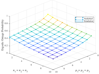
Figure 1: Ergodic outage probability versus the fading parameters $\kappa_{i}$ and $\mu_{i}$, $i\in\left\{1,2,3\right\}$, when $\alpha=0.06$ and $P_{s}=0.5\textrm{W}$.

Now, to illustrate the influence of the EH time factor we present in Fig. 2 the ergodic outage probability with respect to $\alpha$ for the two special cases of the $\kappa$-$\mu$ fading model: Nakagami-$m$ fading in Fig. 2(a) for various values of $\mu$ and Rice fading in Fig. 2(b) with different values of $\kappa$. Note that the numerical results in Figs. 2(a) and 2(b) are obtained from (24) and (23), respectively. It is clear that, for all fading scenarios, when $\alpha$ is either too high or too small, the performance degrades significantly; hence, this parameter must be selected carefully to minimize the outage probability. It is worthwhile pointing out that the results represented by the symbol (+) in Fig. 2(a) are for Rayleigh fading and are obtained from (25).

To illustrate the impact of the loop-back interference channel on the system performance, we plot in Fig. 4 the ergodic outage probability as a function of $P_{s}$ for different values of $\mu_{3}$ when $C_{th}=0.3$bits/s/Hz, $\alpha=0.6$ and $d_{1}=2d_{2}$. Note that, in this figure, we considered a Nakagami-$m$ fading channel and kept $\mu_{1}$ and $\mu_{2}$ fixed at 5. It can be seen that as we improve the loop-back interference channel, i.e., increasing $\mu_{3}$, the performance deteriorates. It is also noticeable that the performance enhances as the transmit power is increased and worsens with increasing the end-to-end distance. Furthermore, Fig. 4 depicts some numerical results of the optimal EH time factor versus the fading parameter $m_{i}$, $i\in\left\{1,2\right\},$ with different values of $\eta$ when $P_{s}=1$W and $m_{3}=3$. Clearly, increasing $m_{i}$ and/or $\eta$ minimizes the outage probability.

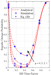
(a) Nakagami-$m$ $\left(\kappa_{1}=\kappa_{2}\rightarrow 0\right)$

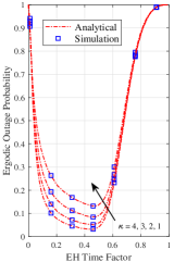
(b) Rice $\left(\mu_{1}=\mu_{2}=1\right)$

Figure 2: Ergodic outage probability versus $\alpha$ for the FD-DF relay system for different $\kappa$ and $\mu$ values.

V Conclusion

This letter analyzed the performance of a FD-DF EH-enabled relaying network over $\kappa$-$\mu$ fading channels. Accurate mathematical expressions were derived for the ergodic outage probability. Three special cases of the $\kappa$-$\mu$ fading were investigated, namely, Rice, Nakagami-$m$ and Rayleigh. Using the derived expressions, the impact of several system parameters were examined such as the fading parameters, loop-back interference channel, end-to-end distance and source transmit power.

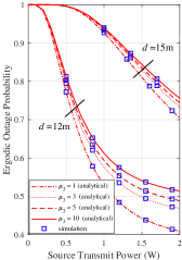
Figure 3: Ergodic outage probability with respect to $P_{s}$ for different loop-back interference scenarios.

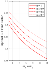
Figure 4: Optimal EH time factor versus the fading parameter $m_{i}$ for different values of $\eta$.

References

• [1] C. Zhong, H. A. Suraweera, G. Zheng, I. Krikidis, and Z. Zhang, “Wireless information and power transfer with full duplex relaying,” IEEE Trans. Commun., vol. 62, pp. 3447–3461, Oct. 2014.
• [2] M. Mohammadi, H. A. Suraweera, G. Zheng, C. Zhong, and I. Krikidis, “Full-duplex MIMO relaying powered by wireless energy transfer,” in Proc. IEEE Int. Workshop Signal Processing Advances in Wireless Commun. (SPAWC), pp. 296–300, Jun. 2015.
• [3] K. M. Rabie, B. Adebisi, and M. S. Alouini, “Half-duplex and full-duplex AF and DF relaying with energy-harvesting in log-normal fading,” IEEE Trans. Green Commun. Netw., vol. 1, pp. 468–480, Dec. 2017.
• [4] G. Nauryzbayev, M. Abdallah, and K. M. Rabie, “Outage probability of the EH-based full-duplex AF and DF relaying systems in $\alpha$-$\mu$ environment,” in Proc. IEEE Veh. Technol. (VTC2018-Fall, 2018, arXiv:1808.02570.
• [5] A. A. Okandeji, M. R. A. Khandaker, K. K. Wong, G. Zheng, Y. Zhang, and Z. Zheng, “Secure full-duplex two-way relaying for SWIPT,” IEEE Wireless Commun. Lett., pp. 1–1, 2017.
• [6] J. Guo, N. Zhao, F. R. Yu, X. Liu, and V. C. M. Leung, “Exploiting adversarial jamming signals for energy harvesting in interference networks,” IEEE Trans. Wireless Commun., vol. 16, pp. 1267–1280, Feb. 2017.
• [7] N. Zhao, Y. Cao, F. R. Yu, Y. Chen, M. Jin, and V. C. M. Leung, “Artificial noise assisted secure interference networks with wireless power transfer,” IEEE Trans. Veh. Technol., vol. 67, pp. 1087–1098, Feb. 2018.
• [8] J. F. Paris, “Outage probability in interference-limited scenarios,” IEEE Trans. Commun., vol. 61, pp. 335–343, Jan. 2013.
• [9] S. Kumar and S. Kalyani, “Coverage probability and rate for $\kappa-\mu/\eta-\mu$ fading channels in interference-limited scenarios,” IEEE Trans. Wireless Commun., vol. 14, pp. 6082–6096, Nov. 2015.
• [10] M. D. Yacoub, “The $\alpha$ - $\eta$ - $\kappa$ - $\mu$ fading model,” IEEE Trans. Antennas and Propagation, vol. 64, pp. 3597–3610, Aug. 2016.
• [11] M. Abramowitz and I. A. Stegun, Handbook of Mathematical Functions with Formulas, Graphs and Mathematical Tables. 1972.
• [12] I. S. Gradshteyn and I. M. Ryzhik, Table of Integrals, Series, and Products. 2007.
• [13] I. S. Gradshteyn and I. M. Ryzhik, Table of Integrals, Series and Products. 6th ed. New York: Academic, 2000.
• [14] A. Nasir, X. Zhou, S. Durrani, and R. Kennedy, “Relaying protocols for wireless energy harvesting and information processing,” IEEE Wireless Commun., vol. 12, no. 7, pp. 3622–3636, Jul. 2013.