Quasi-Chemical Theory with Cluster Sampling from Ab Initio Molecular Dynamics: Fluoride (F^-) Anion Hydration

Abstract

Accurate predictions of the hydration free energy for anions typically have been more challenging than for cations. Hydrogen bond donation to the anion in hydrated clusters such as $\mathrm{F(H_{2}O)}_{n}{}^{-}$ can lead to delicate structures. Consequently, the energy landscape contains many local minima, even for small clusters, and these minima present a challenge for computational optimization. Utilization of cluster experimental results for the free energies of gas phase clusters shows that, even though anharmonic effects are interesting, they need not be troublesome magnitudes for careful applications of quasi-chemical theory to ion hydration. Energy-optimized cluster structures for anions can leave the central ion highly exposed and application of implicit solvation models to these structures can incur more serious errors than for metal cations. Utilizing cluster structures sampled from ab initio molecular dynamics simulations substantially fixes those issues.

I Introduction

Molecular quasi-chemical theory (QCT)^{1; 2; 3; 4; 5; 6; 7} was deliberately developed from molecular statistical thermodynamic theory, and applications have been both simple and remarkably accurate. This situation confronts the canon⁸ of the theory of dense liquids, and begs the question of what accuracy may be achieved as initial simplifications are addressed. The present paper takes up the questions of accuracy of QCT when refined implementations are pursued. Beyond technical theoretical problems, this program brings forward basic questions of operational single-ion free energies underlying rational plans to study specific ion effects.

The basic status of QCT may be supported, but also somewhat camouflaged, by the fact that QCT can be closely coordinated with — indeed implemented through — molecular simulation calculations. ^{9; 10; 11; 12; 13} Earlier works termed that approach ‘direct’ QCT.^{14; 15; 16; 17} On that simulation basis, QCT provides a compelling molecular theory of liquid water itself.^{18; 19; 20; 21; 22; 23; 24; 25; 26} Nevertheless, the initial motivation^{1; 27; 28} was the exploitation of molecular electronic structure calculations in statistical thermodynamic modeling. That approach is called ‘cluster’ QCT.

One motivation for the refinements (below) to cluster QCT is to achieve operational experimental testing of the resulting free energies.²⁹ A practical consequence of that goal is that the QCT should be applied to both cation and anion hydration cases.^{30; 31} Cations interact with ligating atoms with partially negative charge, like oxygens from waters. Recent studies yielded new insights on hydration,^{28; 32; 33; 34; 35; 36; 37; 38; 39}, mechanisms of selective ion binding,^{40; 41; Varma:2008fh; Varma:2010; 42; 43; 45} and specific ion effects for cations.⁴⁴ But anion hydration clusters often exhibit H-bond donation to the ion. Those clusters can be structurally delicate, making hydrated anions more challenging cases.⁴⁶ In the work below, we treat LiF(aq) for the desired testing. For clarity of exposition, we refer to F^-(aq) or Li⁺(aq) when a generic single ion is discussed.

The case of F^-(aq) fits the description above. An initial QCT application works simply with reasonable accuracy.⁴⁶ Nevertheless, refinement of that initial application requires consideration of further technical issues that are taken up here; specifically, quantification of anharmonic effects on free energies of hydrated ion clusters, and the sufficiency of the polarizable continuum model (PCM) for the hydration free energy of those clusters.

QCT Basics

QCT treats the ion-water clusters as molecular species of the system under analysis,^{1; 2; 3; 4; 5; 6; 7} then provides a concise format

$$\mu^{\mathrm{(ex)}}_{\mathrm{F}^{-}}=-RT\ln K^{(0)}_{n}\rho_{\mathrm{H_{2}O}}{}^{n}+RT\ln p_{\mathrm{F}^{-}}(n)\\ +\left(\mu^{\mathrm{(ex)}}_{\mathrm{F(H_{2}O)}_{n}{}^{-}}-n\mu^{\mathrm{(ex)}}_{\mathrm{H_{2}O}}\right)~{},$$ (1)

for free energies of solution components such as F^-(aq). The populations of the clusters are established by applying a clustering algorithm, according to which proximal ligands of a specific ion are defined as inner-shell partners of that ion. The chemical association process,

$$n\mathrm{H_{2}O}+\mathrm{F}^{-}\rightleftharpoons\mathrm{F(H_{2}O)}_{n}{}^{-}~{},$$ (2)

introduces the equilibrium ratio,

$$K_{n}=\frac{p_{{\mathrm{F}^{-}}}(n)}{\rho_{\mathrm{H_{2}O}}{}^{n}p_{{\mathrm{F}^{-}}}(0)}~{},$$ (3)

with $p_{{\mathrm{F}^{-}}}(n)$ as the thermal probability that a specific ion has $n$ inner-shell partners. The factor $K^{(0)}_{n}$ appearing in Eq. (1) is the equilibrium constant $K_{n}$ evaluated for the case that the external medium is an ideal gas. Evaluation of $K^{(0)}_{n}$ is accessible with widely available tools of few-body molecular theoretical chemistry.

Application of QCT to F^-(aq) thus begins with identification of inner-shell configurations of the medium relative to the ion. Emphasizing the observation above that the challenge in treating anions lies in the variety of H-bond donation structures of $\mathrm{F(H_{2}O)}_{n}{}^{-}$, a natural procedure is to identify water molecules with H atoms within a distance of $\lambda$ from F^- as clustered; that is, as inner-shell partners with the distinguished F^- ion. From there, with $n$ water ligands in the cluster and directly interacting with the ion, the free energy is computed using Eq. (1).

For Li⁺(aq), in contrast to F^-(aq), it is natural to identify water molecules with O atoms within a given specific distance from Li⁺ as clustered.

The QCT formula (Eq. (1)) is correct for any physical choices of $\lambda$ and $n$. We emphasize that the combination of terms on the right-side should be independent of $n$. This leads to two further observations. Firstly, for intuitive choices of $\lambda$, the formula Eq. (1) provides a theory of the populations $p_{{\mathrm{F}^{-}}}(n)$ to within a constant, the left-side of Eq. (1); that is, to within post hoc normalization. The most probable value of $n$ provides the minimum value of $\ln p_{{\mathrm{F}^{-}}}(n)$, and it is then natural to simply drop that contribution.

Secondly, the independence of Eq. (1) on $n$ provides an indication of the sufficiency of operational approximations adopted to evaluate the several contributions.

For the leading contribution, $K^{(0)}_{n}$ of Eq. (1), a harmonic approximation for that isolated cluster contribution has been convenient and typically satisfactory. But $K^{(0)}_{n}$ is a characteristic of few-body molecular cluster chemistry, and is available from separate cluster experiments.⁴⁷ Those experimental results permit the work here to avoid that harmonic approximation. In this way, the evaluations below treat anharmonic motion of the clusters considered, and specifically anharmonic zero-point motion, thus further quantifying the significance of the harmonic approximation.

In discussing the various contributions to Eq. (1), we arrive finally at the right-most contribution $\left(\mu^{\mathrm{(ex)}}_{\mathrm{F(H_{2}O)}_{n}{}^{-}}-n\mu^{\mathrm{(ex)}}_{\mathrm{H_{2}O}}\right)$. Here, we will adopt the polarizable dielectric continuum model (PCM).⁴⁸ Although PCM is an extreme approximation, the supporting physical arguments are that electrostatic effects on chemical energy scales clearly dominate more subtle statistical mechanical issues. Moreover, sensitivities to artificial parameters of the PCM, specifically the radii that establish the boundary of the dielectric continuum, are moderated in forming the required difference. Nevertheless, the PCM approximation applied in this combination is the principal approximation of the work below. That again highlights the challenge of treating anions such as F^-. Specifically, if H-bond donation leads to exotic structures for the isolated $\mathrm{F(H_{2}O)}_{n}{}^{-}$ clusters with the ion core highly exposed, that might be a problematic circumstance for the PCM approach. To address this possibility, the work below carries out an inverse sampling approach exploiting the structural results from $ab$ $initio$ molecular dynamics (AIMD) simulations. Those details will be discussed, along with other methods, in the following section.

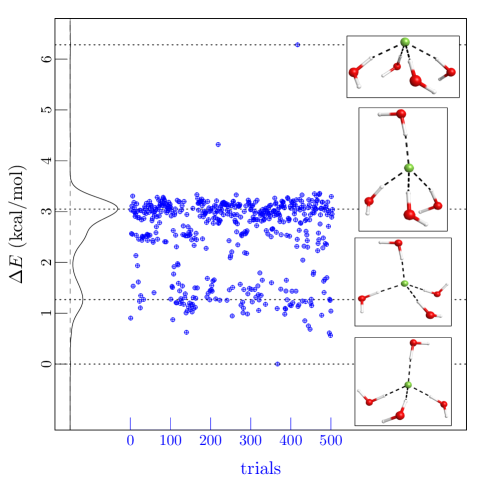
Figure 1: Electronic energy of the optimized $n=4$ clusters (blue dots) starting with configurations sampled from ab initio molecular dynamics. The black curve shows the distribution of these energies. The lowest energy optimum (bottom inset) is about 6 kcal/mol lower in energy than the highest energy optimum (top inset). Harmonic approximation applied to that lowest energy cluster is in good agreement with cluster experiments (FIG. 4).

II Methods

Electronic structure calculations and cluster analysis

All electronic structure calculations were carried out using Gaussian 09 (Rev. D.01).⁴⁹ Geometry optimizations were performed on the $\mathrm{F(H_{2}O)}_{n}{}^{-}$ cluster with 1000 initial cluster configurations sampled from AIMD. The UPBE1PBE⁵⁰ and B3LYP^{51; 52} hybrid density functionals were utilized with the aug-cc-pVDZ⁵³ basis set. Normal mode analysis was then carried out on all 1000 optimized structures to determine zero-point corrected energies and vibrational frequencies.⁵⁴ The absence of imaginary frequencies confirmed that all optimizations resulted in true energy minima.

These calculations also evaluate the single molecule (or cluster) vibrational/rotational partition functions and thus $K^{(0)}_{n}$. Here, the electronic structure calculations analyze rotations of a specific optimized structure without respect to symmetry. Thus, the free energy integrations require some discussion of symmetry numbers for these molecules.^{55; 56} The symmetry number of 2 for the H₂O ligands is elementary and included by hand in our results below.

Considering next the molecular cluster, the general formula for $K^{(0)}_{n}$ presents a $1/n!$ factor,^{1; 3} since the $n$ ligands are treated identically. This factor compensates for the coverage of the ligand conformational space in a general configurational integration. In contrast, the electronic structure calculations exploited here integrate over rotations of a specific cluster structure. The rotational partition functions for a cluster structure might be expected to accomplish, as a practical matter, interchange of the chemically identical ligands. But considering, for example, the case $n$ = 4, rigid body rotations do not achieve inversions of a general structure. Thus, the full permutation group of order $n!$ = 24 is not recovered. Therefore, we simply supply by hand a symmetry number of $n!/2$, 12 rather than 24, for the case $n$ = 4. The case for $n$ = 5, which is considered below, is less simple than $n$=4 and goes beyond merely prescribing the full configurational integration. As an expedient, we use the value of $n!/2$ for that case also.

AIMD simulations

A system consisting of a single fluoride ion and 64 waters was simulated using the VASP AIMD simulation package.^{57; 58} A cubic box of 1.2417 nm was used to match the experimental density of water at standard conditions. The PW91 generalized gradient approximation described the core-valence interactions using the projector augmented-wave (PAW) method. Plane waves with a high kinetic energy cutoff of 400 eV and a time step of 0.5 fs were used for the simulation in an NVE ensemble. A temperature of 350 K was used during the simulation run to avoid glassy behavior that can result at lower $T$.^Rempe:water A total simulation time of 100 ps was run and the last 50 ps trajectory was used for analysis.

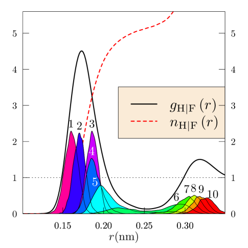
Figure 2: Radial distributions of water H atoms relative to F^- from AIMD. The integer-labeled distributions are the neighborship-ordered contributions of the $n$-th nearest H atom. A choice $\lambda\leq 0.2$ nm excludes split-shell clusters. Note the this neighborship discrimination is sharper here when H-atoms are utilized than when O-atoms were utilized in initial work.⁴⁶

PCM for AIMD sampled clusters

The outer-shell contribution to the hydration free energy $\left(\mu^{\mathrm{(ex)}}_{\mathrm{F(H_{2}O)}_{n}{}^{-}}-n\mu^{\mathrm{(ex)}}_{\mathrm{H_{2}O}}\right)$ is treated using the polarizable continuum model (PCM).⁴⁸ $N_{s}=1000$ $n$-cluster configurations were extracted from the last 50 ps of AIMD simulation, followed by single point electronic energy calculations with PCM as the dielectric medium and separate calculations in the gas phase. The difference, $\varepsilon=\Delta U$, is employed in computing

$$\mu_{\mathrm{F(H_{2}O)}_{n}{}^{-}}^{\mathrm{(ex)}}=RT\ln\left[\left(\frac{1}{N_{s}}\right)\sum\limits_{j=1}^{N_{s}}\mathrm{e}^{\varepsilon_{j}/RT}\right].$$ (4)

This approach corresponds to the PDT formula^{3; 59} for the inverse case, that is, particle deletion. We explicitly verified that these PCM results were insensitive to the specific value of the solution dielectric constant in a high $\epsilon$ range relevant to liquid water; the $\epsilon\rightarrow\infty$ could have been used with imperceptible difference. Therefore, although the configurations sampled here correspond to AIMD trajectories at 350 K, we expect the differences in PCM-single-point energies at 298 K to be small. Those differences could, of course, be studied in future work.

In PCM, the boundary around the solute is defined by spheres centered on each of the atoms. The sensitivity of the outer-shell contribution to the size of this cavity is characterized by changing the radius, $R_{\mathrm{F}^{-}}$, of the solute atom between 0.15 nm and 0.20 nm. Our operational value was $R_{\mathrm{F}^{-}}=0.169$ nm, the default PCM radius. That radius lies close to the maximum in the radial distribution of water hydrogens about the anion (FIG. 2).

III Results

Clustering constraint and solution structure

The arrangements of ligands around a solute guide our assignment of the clustering radius, $\lambda$. The radial distribution function of water-H atoms relative to F^-, when resolved into neighborship-ordered contributions, clarify those considerations (FIG. 2). Notice that the 6th-nearest neighbor distribution is bimodal, with peaks on both sides of the minimum of $g_{\mathrm{H|F}}\left(r\right)$. A choice of $\lambda\leq 0.20$ nm excludes such split-shell occupancies,^{46; 37} that is, waters that are not always in direct contact with the ion. The thermal probability, $p_{\mathrm{F}^{-}}(n)$, contributing to the second term of Eq. (1), is then evaluated based on this constraint.

Accuracy of the harmonic approximation

We extracted $N_{s}=1000$ $n$-clustered configurations from the last 50 ps of AIMD simulations and optimized their geometries with respect to energy in the gas phase (FIG. 1,3). Only cluster sizes with $2\leq n\leq 5$ were observed for $\lambda=0.2$ nm. For the case of $n=4$, optimized energies span a range of 1-3 kcal/mol in a bimodal fashion (FIG. 1). Those energy differences are attributed to subtle changes in the orientations of the ligands.

For $n=5$, some optimizations pushed a water molecule out to form structures that we label henceforth as “4+1” (bottom inset). The rest are “5+0” optimized clusters (top inset). The “4+1” structures violate the clustering constraint and are not included in evaluation of the free energy. This issue does not arise for clusters with $n\leq 4$.

Finally, $-RT\ln K^{(0)}_{n}$ is evaluated within a harmonic assumption for the lowest energy structure (FIG. 4). Comparison with cluster experiments⁴⁷ indicates accurate agreement for cluster sizes $n\leq 4$. The $n=5$ case suggests that the “4+1” structures contribute importantly to these experiments, as also found earlier for sodium.⁶⁰ The B3LYP functional, which performs better in this comparison, is adopted for further analyses that include outer-shell contributions.

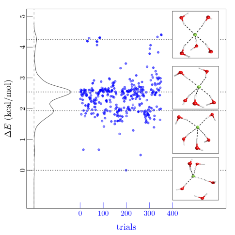
Figure 3: Electronic energy of the optimized $n=5$ clusters (blue dots) starting with configurations sampled from ab initio molecular dynamics. The black curve shows the distribution of these energies. Two kinds of optimized structures are observed here. Lowest energy, ‘split-shell’ (4+1) structures (bottom inset), which do not obey the clustering constraint, are the first kind. The lowest energy (5+0) structures are the second kind and they conform to the clustering constraint on which QCT theory is developed.

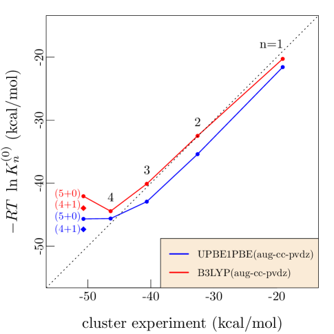
Figure 4: Evaluation of $-k_{\mathrm{B}}T\ln K^{(0)}_{n}$ using the harmonic approximation agrees well with cluster experiments⁴⁷ for cluster sizes $n\leq 4$. For $n=5$, the results suggest that (4+1) structures contribute importantly to these experiments. Anharmonicity effects likely make less specific, more quantitative contributions elsewhere.⁶¹ The B3LYP functional, which performs better here, is adopted for further analyses including outer-shell contributions.

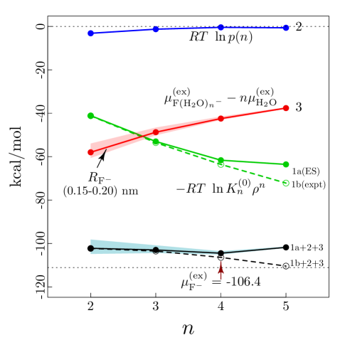
Figure 5: Topmost: The free energy contribution related to cluster poly-dispersity. Red: The outer shell contribution to the hydration free energy evaluated using the PCM model.⁴⁸ The red band is obtained by varying $R_{\mathrm{F}^{-}}$, as indicated in the text. Green: Isolated cluster free energy (FIG. 4), with the corresponding dashed curve from cluster experiments.⁴⁷ Black: The excess free energy of hydration for F^-, $\mu^{\mathrm{(ex)}}_{\mathrm{F}^{-}}$, evaluated using Eq. (1). The sum of these contributions is substantially independent of $n$. The black dotted line ($-111.1$ kcal/mol) is the value tabulated by Marcus.⁶²

IV Discussion

Anharmonic effects on cluster free energies are easy to observe and interesting (FIGS. 1 & 3). Even for such a small cluster as F(H₂O)${}_{4}{}^{-}$, the energy landscape has many local minima. These minima are a challenge for computational optimization. Nevertheless, comparison of theoretical results with experimental assessment of anharmonic effects, and including zero-point motion on that basis, shows that the differences for cluster free energies are not troublesome for this QCT application (FIG. 4, 5).

The sum of the several QCT contributions for F^-(aq) (FIG. 5) is substantially independent of $n$, which adds confidence to the QCT results. The predicted hydration free energy ($-106.4$ kcal/mol) is in good agreement with experimental tabulation of Marcus ($-111$ kcal/mol).⁶²

A similar QCT analysis for Li⁺(aq) arrives at a value of $-121.1$ kcal/mol for $\mu^{\mathrm{(ex)}}_{\mathrm{Li}^{+}}$ (see Supplementary Information). Then the QCT prediction for the neutral combination, $\mu_{\mathrm{F^{-}}}^{\mathrm{(ex)}}+\mu_{\mathrm{Li^{+}}}^{\mathrm{(ex)}}$ = $-227.5$ kcal/mol, is in fair agreement with experimental tabulations, which range between $-229$ kcal/mol and $-232$ kcal/mol.^{29; 63; 62; 47} Issues of a surface potential are not involved in this comparison.^{Leung:2009dx; Rempe:2010er}

V Conclusions

The use of the PCM implicit solvation model is simple and physically natural, but is ultimately the most serious approximation for QCT applications to anions in water. On the one hand, the simplest QCT application results in the central ion well-covered with inner-shell ligands before relying on a traditional PCM approximation. On the other hand, energy-optimized cluster structures for anions can leave the central ion highly exposed. Application of PCM to those structures incurs more serious errors than for metal cations. Cluster sampling from ab initio molecular dynamics substantially fixes that issue with the standard QCT application. The QCT results obtained that way for LiF, a neutral combination so not involving a surface potential,⁶⁴ shows fair agreement with experimental free energies. We emphasize that we do not address here the partial molar volumes of simple ions in water on this basis of QCT, though the ground-work for that next challenge was laid many years ago.¹

VI Acknowledgment

Sandia National Laboratories is a multimission laboratory managed and operated by National Technology & Engineering Solutions of Sandia, LLC, a wholly owned subsidiary of Honeywell International Inc., for the U.S. Department of Energy’s National Nuclear Security Administration under contract DE-NA0003525. This work was supported by Sandia’s LDRD program. This work was performed, in part, at the Center for Integrated Nanotechnologies (CINT), an Office of Science User Facility operated for the U.S. DOE’s Office of Science by Los Alamos National Laboratory (Contract DE-AC52-06NA25296) and SNL. The views expressed in the article do not necessarily represent the views of the U.S. Department of Energy or the United States Government.

References

- Pratt and Rempe (1999) L. R. Pratt and S. B. Rempe, in Simulation and Theory of Electrostatic Interactions in Solution, edited by G. Hummer and L. R. Pratt (AIP: New York, 1999) pp. 177–201.
- Paulaitis and Pratt (2002) M. E. Paulaitis and L. R. Pratt, Adv. Prot. Chem. 62, 283 (2002).
- Beck, Paulaitis, and Pratt (2006) T. L. Beck, M. E. Paulaitis, and L. R. Pratt, The Potential Distribution Theorem and Models of Molecular Solutions (Cambridge University Press, 2006).
- Pratt and Asthagiri (2007) L. R. Pratt and D. Asthagiri, in Free Energy Calculations (Springer, 2007) pp. 323–351.
- Asthagiri et al. (2010) D. Asthagiri, P. D. Dixit, S. Merchant, M. E. Paulaitis, L. R. Pratt, S. B. Rempe, and S. Varma, Chem. Phys. Lett. 485, 1 (2010).
- Rogers and Rempe (2011) D. M. Rogers and S. B. Rempe, J. Phys. Chem. B 115, 9116 (2011).
- Rogers et al. (2013) D. M. Rogers, D. Jiao, L. R. Pratt, and S. B. Rempe, Ann. Rep. Comp. Chem. 8, 71 (2013).
- Chandler, Weeks, and Andersen (1983) D. Chandler, J. D. Weeks, and H. C. Andersen, Science 220, 787 (1983).
- Tomar, Asthagiri, and Weber (2013) D. S. Tomar, D. Asthagiri, and V. Weber, Biophys. J. 105, 1482 (2013).
- Tomar et al. (2014) D. S. Tomar, V. Weber, B. M. Pettitt, and D. Asthagiri, J. Phys. Chem. B 118, 4080 (2014).
- Tomar et al. (2015) D. S. Tomar, V. Weber, B. M. Pettitt, and D. Asthagiri, J. Phys. Chem. B 120, 69 (2015).
- Asthagiri et al. (2017) D. Asthagiri, D. Karandur, D. S. Tomar, and B. M. Pettitt, J. Phys. Chem. B 121, 8078 (2017).
- Tomar, Ramesh, and Asthagiri (2018) D. S. Tomar, N. Ramesh, and D. Asthagiri, J. Chem. Phys. 148, 222822 (2018).
- Sabo et al. (2008) D. Sabo, S. Varma, M. G. Martin, and S. B. Rempe, J. Phys. Chem. B 112, 867 (2008).
- Jiao and Rempe (2011) D. Jiao and S. B. Rempe, J. Chem. Phys. 134, 224506 (2011).
- Chaudhari et al. (2015) M. I. Chaudhari, D. Sabo, L. R. Pratt, and S. B. Rempe, J. Phys. Chem. B 119, 9098 (2015).
- Chaudhari, Pratt, and Rempe (2018) M. I. Chaudhari, L. R. Pratt, and S. B. Rempe, Mol. Simul. 44, 110 (2018).
- Asthagiri, Pratt, and Kress (2003) D. Asthagiri, L. R. Pratt, and J. Kress, Phys. Rev. E 68, 041505 (2003).
- Paliwal et al. (2006) A. Paliwal, D. Asthagiri, L. Pratt, H. Ashbaugh, and M. Paulaitis, J. Chem. Phys. 124, 224502 (2006).
- Shah et al. (2007) J. Shah, D. Asthagiri, L. Pratt, and M. Paulaitis, J. Chem. Phys. 127, 144508 (2007).
- Chempath and Pratt (2008) S. Chempath and L. R. Pratt, J. Phys. Chem. B 113, 4147 (2008).
- Chempath, Pratt, and Paulaitis (2009) S. Chempath, L. R. Pratt, and M. E. Paulaitis, J. Chem. Phys. 130, 054113 (2009).
- Weber et al. (2010) V. Weber, S. Merchant, P. D. Dixit, and D. Asthagiri, J. Chem. Phys. 132, 204509 (2010).
- Weber and Asthagiri (2010) V. Weber and D. Asthagiri, J. Chem. Phys. 133, 141101 (2010).
- Weber, Merchant, and Asthagiri (2011) V. Weber, S. Merchant, and D. Asthagiri, J. Chem. Phys. 135, 181101 (2011).
- Merchant, Shah, and Asthagiri (2011) S. Merchant, J. K. Shah, and D. Asthagiri, J. Chem. Phys. 134, 124514 (2011).
- Martin, Hay, and Pratt (1998) R. L. Martin, P. J. Hay, and L. R. Pratt, J. Phys. Chem. A 102, 3565 (1998).
- Rempe et al. (2000) S. B. Rempe, L. R. Pratt, G. Hummer, J. D. Kress, R. L. Martin, and A. Redondo, J. Am. Chem. Soc. 122, 966 (2000).
- Friedman and Krishnan (1973) H. Friedman and C. Krishnan, in Aqueous Solutions of Simple Electrolytes (Springer, 1973) pp. 1–118.
- Beck (2013) T. L. Beck, Chem. Phys. Letts. (2013).
- Chaudhari et al. (2018) M. I. Chaudhari, J. M. Vanagas, L. R. Pratt, and S. B. Rempe, Acc. Chem. Res. (2018).
- Rempe and Pratt (2001) S. B. Rempe and L. R. Pratt, Fl. Ph. Equ., 183–184, 121 (2001).
- Rempe, Asthagiri, and Pratt (2004) S. B. Rempe, D. Asthagiri, and L. R. Pratt, Phys. Chem. Chem. Phys. 6, 1966 (2004).
- Asthagiri et al. (2004) D. Asthagiri, L. R. Pratt, M. E. Paulaitis, and S. B. Rempe, J. Am. Chem. Soc. 126, 1285 (2004).
- Jiao et al. (2011) D. Jiao, K. Leung, S. B. Rempe, and T. M. Nenoff, J. Chem. Theo. Comp. 7, 485 (2011).
- Alam, Hart, and Rempe (2011) T. M. Alam, D. Hart, and S. L. B. Rempe, Phys. Chem. Chem. Phys. 13, 13629 (2011).
- Sabo et al. (2013) D. Sabo, D. Jiao, S. Varma, L. R. Pratt, and S. B. Rempe, Ann. Rep. Prog. Chem, Sect. C (Phys. Chem.) 109, 266 (2013).
- Mason et al. (2015) P. E. Mason, S. Ansell, G. W. Neilson, and S. B. Rempe, J. Phys. Chem. B 119, 2003 (2015).
- Chaudhari, Soniat, and Rempe (2015) M. I. Chaudhari, M. Soniat, and S. B. Rempe, J. Phys. Chem. B 119, 8746 (2015).
- Varma and Rempe (2007) S. Varma and S. B. Rempe, Biophys. J. 93, 1093 (2007).
- Varma, Sabo, and Rempe (2008) S. Varma, D. Sabo, and S. B. Rempe, J. Mol. Bio. 376, 13 (2008).
- Varma et al. (2011) S. Varma, D. M. Rogers, L. R. Pratt, and S. B. Rempe, J. Gen. Phys. 137, 479 (2011).
- Rossi et al. (2013) M. Rossi, A. Tkatchenko, S. B. Rempe, and S. Varma, Proc. Natl. Acad. Sci. U.S.A. 110, 12978 (2013).
- Stevens and Rempe (2016) M. Stevens and S. B. Rempe, J. Phys. Chem. B 120, 12519 (2016).
- Chaudhari and Rempe (2018) M. I. Chaudhari and S. B. Rempe, J. Chem. Phys. , 222831 (2018).
- Chaudhari, Rempe, and Pratt (2017) M. I. Chaudhari, S. B. Rempe, and L. R. Pratt, J. Chem. Phys. 147, 161728 (2017).
- Tissandier et al. (1998) M. D. Tissandier, K. A. Cowen, W. Y. Feng, E. Gundlach, M. H. Cohen, A. D. Earhart, J. V. Coe, and T. R. Tuttle, J. Phys. Chem. A 102, 7787 (1998).
- Tomasi, Mennucci, and Cammi (2005) J. Tomasi, B. Mennucci, and R. Cammi, Chem. Rev. 105, 2999 (2005).
- Frisch et al. (1998) M. Frisch, G. Trucks, H. Schlegel, G. Scuseria, M. Robb, J. Cheeseman, V. Zakrzewski, J. Montgomery Jr, R. Stratmann, J. Burant, et al., Pittsburgh, Pa 40 (1998).
- Perdew, Burke, and Ernzerhof (1996) J. P. Perdew, K. Burke, and M. Ernzerhof, Phys. Rev. Letts. 77, 3865 (1996).
- Becke (1993) A. D. Becke, J. Chem. Phys. 98, 5648 (1993).
- Lee, Yang, and Parr (1988) C. Lee, W. Yang, and R. G. Parr, Phys. Rev. B 37, 785 (1988).
- Dunning Jr (1989) T. H. Dunning Jr, J. Chem. Phys. 90, 1007 (1989).
- Rempe and Jónsson (1998) S. B. Rempe and H. Jónsson, Chem. Educator 3, 1 (1998).
- Ochterski (2000) J. W. Ochterski, Thermochemistry in gaussian (Gaussian Inc, 2000).
- Irikura (1998) K. K. Irikura, Computational Thermochemistry Prediction and Estimation of Molecular Thermodynamics, edited by K. K. Irikura and D. J. Frurip, Vol. 677 (ACS Symposium Series, 1998).
- Kresse and Hafner (1993) G. Kresse and J. Hafner, Physical Review B 47, 558 (1993).
- Kresse and Furthmüller (1996) G. Kresse and J. Furthmüller, Physical review B 54, 11169 (1996).
- Dullens et al. (2005) R. P. Dullens, D. G. Aarts, W. K. Kegel, and H. N. Lekkerkerker, Mol. Phys. 103, 3195 (2005).
- Soniat, Rogers, and Rempe (2015) M. Soniat, D. M. Rogers, and S. B. Rempe, J. Chem. Theory Comput. 11, 150626121718001 (2015).
- Kathmann, Schenter, and Garrett (2007) S. Kathmann, G. Schenter, and B. Garrett, J. Phys. Chem. C 111, 4977 (2007).
- Marcus (1994) Y. Marcus, Biophys. Chem. 51, 111 (1994).
- Hünenberger and Reif (2011) P. Hünenberger and M. Reif, Single-Ion Solvation: Experimental and Theoretical Approaches to Elusive Thermodynamic Quantities, Vol. 3 (Royal Society of Chemistry, 2011).
- You, Chaudhari, and Pratt (2014) X. You, M. Chaudhari, and L. Pratt, in Aqua Incognita: Why Ice Floats on Water and Galileo 400 Years on (Connor Court Press Ballarat, 2014) pp. 434–442, Comparison of Mechanical and Thermodynamical Evaluations of Electrostatic Potential Differences between Electrolyte Solutions.