An open-source finite volume toolbox for solid mechanics and fluid-solid interaction simulations

Abstract

Over the past 30 years, the cell-centred finite volume method has developed to become a viable alternative to the finite element method in the field of computational solid mechanics. The current article presents an open-source toolbox for solid mechanics and fluid solid interaction simulations based on the finite volume library OpenFOAM^®. The object oriented toolbox design is outlined, where emphasis has been given to code use, comprehension, maintenance and extension. The toolbox capabilities are demonstrated on a number of representative test problems, where comparisons are given with finite element solutions.

1 Introduction

Numerical analysis techniques, such as the finite element (FE) and finite volume (FV) methods, have found widespread use in modern engineering industry and academia, ranging from component design to the analysis of physical mechanisms. For multi-physics problems, there are a number of viable commercial software options; however, there has been relatively little development of open-source software for this purpose. In particular, there are few open-source packages that offer significant fluid and solid analysis capabilities within the same framework.

The FE method dominates the field of computational solid mechanics (CSM), whereas the FV method is the most popular technique for computational fluid dynamics (CFD); this poses a significant challenge for problems which involve both fluid-like and solid-like materials. Coupling of separate analysis packages and techniques is an option; however, performing such multi-physics analyses within a consistent software framework offers a number of advantages in terms of code development and solver efficiency.

In the past decade, open-source software OpenFOAM has become one of the most popular packages in the realm of CFD and multi-physics simulations. The OpenFOAM project emerged from the Field Operations And Manipulations (FOAM) concept at Imperial College London in the late-1980s. As stated by Weller et al. [1], an aim of the project was “to make it as easy as possible to develop reliable and efficient computational continuum-mechanics codes”; this was achieved by exploiting newly developed object-oriented design paradigms, and making the top-level syntax closely resemble conventional mathematical notation for partial differential equations; combined with native parallelisation support and the open-source GPL license [2], this has lead to the widespread adoption of OpenFOAM in academia and industry, for example, [3, 4].

Although OpenFOAM has seen significant developments across the entire domain of CFD applications, the establishment of procedures for CSM and fluid-solid interactions (FSI) is still nascent, contributed to by the general lack of personnel with combined CFD and CSM expertise. In the formative publications on OpenFOAM, Weller et al.[1, 5] presented analysis of the classical hole in an elastic plate problem, where the cell-centred FV discretisation built on the pioneering work of Demirdžić and co-workers [6, 7, 8]. Subsequently, within the OpenFOAM framework, there have been a number of extensions to the cell-centred FV methods for CSM, as regards finite strains [9, 10, 11, 12], constitutive relations [13, 10, 11, 14], boundary conditions [15, 16, 17, 18, 19], discretisation and solution methodologies [20, 21, 22, 23], as well as FSI approaches, notably [24, 25, 26, 27, 28, 29, 30, 31, 32, 33, 34].

Apart from Tuković et al. [30, 34], the previous works all focused on the development of bespoke numerical procedures, where no emphasis was placed on the creation of generalised code structures that may be easily combined, adapted and extended to related CSM and FSI problems. In particular, little attention has been given to the development of modular designs, allowing straight-forward combination of differing solid and fluid procedures for FSI problems, or allowing for the addition of new solid constitutive relations, for example. The official versions of OpenFOAM are released with only the most basic solid mechanics tools, specifically the solidDisplacementFoam solver, which is restricted to Hookean solids undergoing small strains and rotations. The current article aims to overcome these shortcomings by presenting and sharing a solid mechanics and FSI toolbox built on OpenFOAM software framework. The adopted approach aims to follow object-oriented design principles that allow for straight-forward use, comprehension, extension, and maintenance of the code. Furthermore, the toolbox will be made freely available to the community via the FOAM Extend community fork [35] and the OpenFOAM Community Repository [36], such that the implementations are fully open to academic scrutiny and allow future collaborative improvements.

The article is structured as follows: Section 2 gives an overview of the toolbox design; Section 3 summarises the mathematical models that are solved; Section 4 outlines the cell-centred FV discretisation and solution methodologies; in Section 5, a number of test cases are presented, highlighting the capabilities and applicability of the toolbox; finally, Section 6 briefly discusses the presented methods in light of conventional FE methods and indicates future directions.

2 Toolbox Structure & Design

Over the past half century, there has been extensive literature published on the development of discretisations, solution methodologies and algorithms within the field of computational mechanics; however, relatively little importance has been given to code design: this is somewhat understandable given the procedures are typically developed by engineers and applied mathematicians as opposed to computer programmers. As the complexity of modern parallelised multi-physics procedures continues to increase, good code design becomes ever more crucial to the solution of complex problems. Historically, procedural programming implementations were favoured, for example, in FOTRAN, but due to the proliferation of object-oriented programming (OOP) languages, such as C++ in the 1990s, there has been a gradual turn to the benefits of such abstract programming paradigms. One of the key characteristics of procedural programming is that it relies on procedures that operate on data; in contrast, these two separate concepts are bundled into objects in OOP approaches: this makes it possible to create complex behaviour with less code and less repetition of code.

With the development of OpenFOAM, Weller et al. [1] was one of the first to place specific emphasis on the design philosophy of an engineering analysis tool for CFD; the philosophy of OOP was embraced, where conceptual constructs (a class) are represented in the program, with specific details hidden behind an interface with limited, well-defined access; in this way, data types are created that represent, for example, tensor fields allowing the governing partial differential equations to be constructed in a manner similar to their mathematical counterparts. Numerical details - irrelevant at this level - are hidden by encapsulation (contain and protect the data that make up the class). There are a number of other notable works that have emphasised the software design element of an engineering tool, for example, Archer [37], van Riesen et al. [38], Bangerth et al. [39], and Palacios et al. [40].

As OpenFOAM is released under the open-source GPL license [2], it lends itself to the development of add-on toolboxes, such as a wave generation toolbox by Jacobsen et al. [41], a toolbox for modelling soil-structure interaction around marine structures by Elsafti and Oumeraci [22], and a porous media flow toolbox by Horgue et al. [42]; in a similar fashion, the current article presents here a toolbox, titled solids4foam, which aims to generalise the OpenFOAM design further to allow straightforward implementation of advanced solid mechanics and fluid-solid interaction procedures. Throughout the design the solids4foam, significant emphasis has been placed on the following complementary factors:

• usable: the solvers should be intuitive for a new user to use;

• understandable: the code structure should be easy to follow for a developer who is not familiar with the project, where esoteric structures are avoided; for example, class, data and function names should be descriptive, and a consistent style convention should be adopted;

• maintainable: the design should enable straightforward maintenance, in particular as the code grows and features are added; modularisation should be embraced and code repetition should be avoided;

• extendable: the design should allow key features to be extended in a straight-forward manner, particularly for unfamiliar developers, for example, adding a new constitutive relation, solution methodology or boundary condition.

In the subsequent sections, these four points are addressed through the design and structure of the presented solids4foam toolbox.

2.1 Design of the class structure

In the standard OpenFOAM public release, there are a large number of solver executables, each designed for a specific group of problems, for example, laplacianFoam solves the transient Laplace equation (heat conduction), icoFoam solves the isothermal laminar Newtonian incompressible Navier-Stokes equations and solidDisplacementFoam solves the small strains/rotations Hookean elastic equations; this approach has a number of merits relative to the single executable design approach; however, it has its limitations when considering coupled physics problems. Consider a fluid-solid interaction problem where we wish to combine any one of the fluid models with any one of the solid models, for example, a compressible turbulent multiphase fluid with a visco-elastic neo-Hookean solid. To overcome such a limitation, the current article builds on the framework of Tuković et al.[30, 34] to propose a modular design structure where solution methodologies are encapsulated within classes; for example, the Pressure-Implicit with Splitting of Operators (PISO) solution algorithms for fluids, or the total Lagrangian nonlinear geometry solution algorithm for solids.

The top level class structure of solids4foam is shown in Figure 1, where the UML notation [43] is broadly followed; as indicated, the Physics Model class represents a mathematical model (boundary value problem), for either a solid or fluid or fluid-solid problem. At run-time the user specifies which specific implementation will be invoked, via user input files; in this way, the Physics Model is a so-called abstract base class, from which Solid Models, Fluid Models and Fluid-Solid Interaction Models are derived. This demonstrates the OOP concept of polymorphism, where classes can be considered conceptually equivalent and share the same interface but have different implementations; for example, at run-time the user can switch between a mathematical model for a solid that assumes small strains (linear geometry) and a mathematical model valid for finite strains (nonlinear geometry), or switch between a segregated and block-coupled solution methodology.

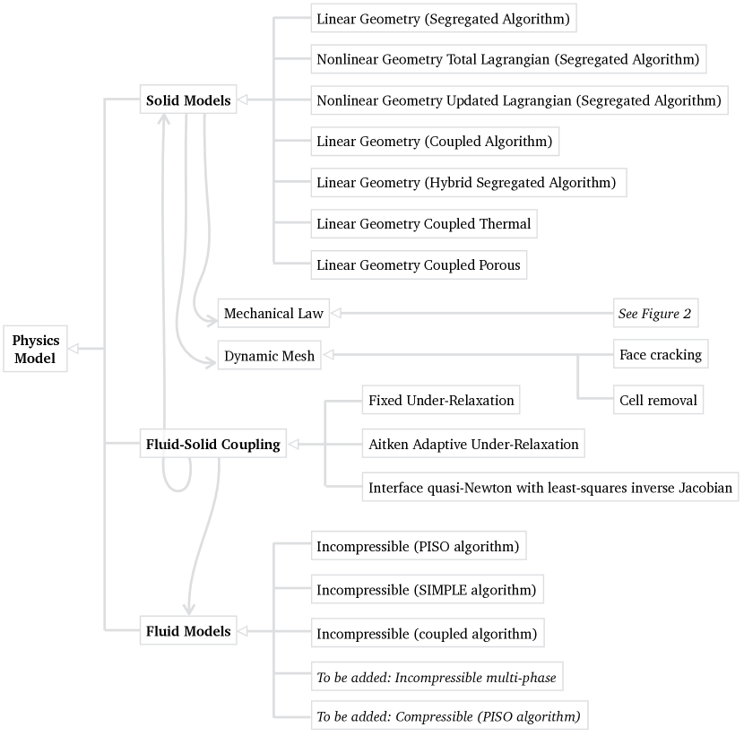
Figure 1: Class structure: fluid, solid, and fluid-solid interaction mathematical models

In Figure 1, the lines with a closed, unfilled arrowhead indicate an inheritance relationship between classes: for example, the Linear Geometry (Segregated Algorithm) class inherits the attributes of the Solid Model class, and similarly the Solid Model class inherits the attributes of the Physics Model class; in this way, inheritance enables commonality relationships to be expressed between classes. It should be noted that the polymorphism and inheritance mechanisms are effective methods to minimise code duplication (i.e. repeating segments of code in multiple places), which is a critical point to ensure the code maintainability. In addition, such a system allows straightforward addition of new derived classes, for example, consider the mechanical constitutive law classes in Figure 2. Lines ending in open arrowheads (for example, from the Mechanical Law to the Solid Model) indicates a uni-directional association; in such an association, the two classes are related, but only one class knows that the relationship exists; for example, the Solid Model class contains a Mechanical Law, which is required to calculate the stress tensor field; however, the Mechanical Law class need not know about how the specific solid model solution algorithm is implemented and should only be concerned with the calculation of the stress field when asked. This demonstrates the concept of encapsulation where a Mechanical Law derived class, such as Linear (Hookean) elastic, encapsulates and protects data specific to the law (for example, Young’s modulus and Poisson’s ratio) and only provides access through a well defined interface (for example, calculate the stress given the strain or deformation gradient field).

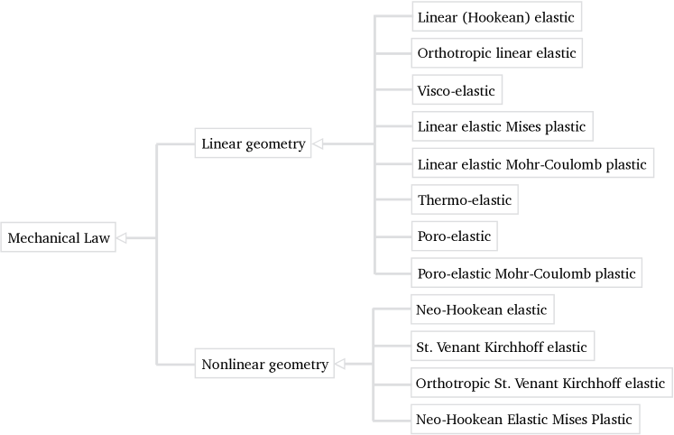
Figure 2: Class structure: mechanical laws and dynamic meshes

The class structure and design presented in Figures 1 and 2 takes advantage of design patterns commonly used in OOP; further discussion of design patterns can be found in [44]. The use of such design patterns can speed up the development process by providing tested, proven development paradigms; in addition, the reuse of design patterns helps improve code readability for those familiar with the patterns. In this case the so-called factory method [44] is exploited multiple times, where a parent class defines an interface for creating objects, but lets subclasses decide which classes to instantiate; for example, the Solid Model parent class defines the interfaces but derived classes such as Linear Geometry (Segregated Algorithm) define the actual implementation. Considerable time has been given to consider future extensions that may occur and ensuring the code design is sufficiently flexible to allow for this; however, the code base is not static and continues to evolve; as such, the habit of refactoring continuously will allow easier extension and maintenance; in this sense, refactoring refers to the process of restructuring existing computer code without changing its external behaviour, in an attempt to improve code readability and reduce complexity.

2.2 Note on Style, Revision Control & Documentation

As the solids4foam toolbox is presented to the community as an open-source repository, users and developers from other institutions are invited to contribute; consequently, to ensure that the toolbox does not become a patchwork quilt of contrasting styles making the code difficult to read, it is critical to enforce stringent coding standards; strict enforcement of such coding standards ensures the software is easy to read, maintain and extend. Following such standards immediately ensures code is more readable and understandable, allowing faster and more error-free developments; in addition, when coding standards are not followed, reading code generated by others becomes a tedious, painstaking and even an impossible task. Fortunately, the developers of the public release of OpenFOAM have set out a comprehensive coding style [45]; this style is strictly followed in the solids4foam toolbox.

A Git revision control system is used to track changes to the source code, both on the local repository as well as within the open-source published source code. Doxygen code documentation provides developers with the code structure and interfaces.

2.3 Note on the open-source paradigm

Commercial engineering software offers notable capabilities as regards the implementation of custom user routines; however, the development and implementation of novel solution procedures is not possible without access to the code base. For those interested in such developments, whether for academic or industrial reasons, one option is to develop code in-house. This overcomes the limitations of commercial software; however, it has the drawback that the documentation, maintenance and extension of the code can be difficult due to the small in-house user base. A potentially more appealing option is starting from a suitable open-source library with a significant user base; this potentially increases the speed of developing new procedures as well as allowing the reuse of code provided by the community. An additional benefit of the open-source paradigm is that the code base is fully open to academic scrutiny, where normal users are granted a complete view into the source code; this provides access to which algorithms are implemented, and more importantly how they are implemented. Within such an open-source framework, large scale community collaborations become possible, and development of complex multi-physics procedures can proceed at an accelerated rate.

Open-source software is, of course, not without its weaknesses: it requires a certain level of system administration experience and technical expertise in order to manage and develop content; in addition, there are often no official code reviews or quality assurance processes in place, instead relying on users and developers to perform these verifications, checks and subsequent fixes. Nevertheless, open-source software projects certainly possess a number of advantageous features suitable for the development of state-of-the-art numerical procedures.

3 Mathematical Models

In this section, an overview is given of the mathematical models that are solved in the Solid Model, Fluid Model and Fluid-Solid Interaction classes. As the fluid models and FSI interaction procedures have been extensively described previously, for example, [1, 34], emphasis is given here to the description of the solid model methods.

3.1 Governing Equations

Considering an arbitrary body of volume $\Omega$ bounded by surface $\Gamma$ with outward facing normal $\boldsymbol{n}$, the governing equations - conservation of mass, conservation of energy (heat equation form) and conservation of linear momentum - are given in strong integral form as:

$$\frac{\text{D}}{\text{D}t}\int_{\Omega}\rho\;\text{d}\Omega=0$$ (1)

$$\frac{\text{D}}{\text{D}t}\int_{\Omega}\rho C_{p}T\;\text{d}\Omega\;=\;-\oint_{\Gamma}\boldsymbol{n}\cdot\boldsymbol{q}\;\text{d}\Gamma\;+\;\int_{\Omega}\boldsymbol{\sigma}:\boldsymbol{\nabla}\boldsymbol{v}\;\text{d}\Omega$$ (2)

$$\frac{\text{D}}{\text{D}t}\int_{\Omega}\rho\boldsymbol{v}\;\text{d}\Omega\;=\;\oint_{\Gamma}\boldsymbol{n}\cdot\boldsymbol{\sigma}\;\text{d}\Gamma\;+\;\int_{\Omega}\rho\,\boldsymbol{b}\;\text{d}\Omega$$ (3)

where $\rho>0$ is the density, $C_{p}>0$ is the specific heat capacity at constant pressure, $T$ is the temperature, $\boldsymbol{q}$ is the heat flux vector, $\boldsymbol{\sigma}$ is the Cauchy stress tensor, $\boldsymbol{v}$ is the velocity vector, and $\boldsymbol{b}$ is the body force per unit mass; symbol $\boldsymbol{\nabla}$ signifies the so called Hamilton operator, synonymous with the del or nabla operator. In addition, the necessary and sufficient condition for the conservation of angular momentum is the symmetry of the Cauchy stress tensor.

Employing Reynold’s transport theorem, the total derivatives may be replaced by partial derivatives as:

$$\frac{\partial}{\partial t}\int_{\Omega}\rho\;\text{d}\Omega\;+\;\oint_{\Gamma}\rho\left[\boldsymbol{n}\cdot(\boldsymbol{v}-\boldsymbol{v}_{\Gamma})\right]\;\text{d}\Gamma=0$$ (4)

$$\frac{\partial}{\partial t}\int_{\Omega}\rho CT\;\text{d}\Omega\;+\;\oint_{\Gamma}\rho CT\left[\boldsymbol{n}\cdot(\boldsymbol{v}-\boldsymbol{v}_{\Gamma})\right]\;\text{d}\Gamma\;=\;-\oint_{\Gamma}\boldsymbol{n}\cdot\boldsymbol{q}\;\text{d}\Gamma\;+\;\int_{\Omega}\boldsymbol{\sigma}:\boldsymbol{\nabla}\boldsymbol{v}\;\text{d}\Omega$$ (5)

$$\frac{\partial}{\partial t}\int_{\Omega}\rho\boldsymbol{v}\;\text{d}\Omega\;+\;\oint_{\Gamma}\rho\boldsymbol{v}\left[\boldsymbol{n}\cdot(\boldsymbol{v}-\boldsymbol{v}_{\Gamma})\right]\;\text{d}\Gamma\;=\;\oint_{\Gamma}\boldsymbol{n}\cdot\boldsymbol{\sigma}\;\text{d}\Gamma\;+\;\int_{\Omega}\rho\,\boldsymbol{b}\;\text{d}\Omega$$ (6)

where $\boldsymbol{v}_{\Gamma}$ is the velocity of the control volume surface $\Gamma$. As yet, no distinction has been made between solid and fluid materials; the difference comes in the assumed constitutive relations, for example, in the definition of the Cauchy stress $\boldsymbol{\sigma}$. In addition, for convenience a Lagrangian approach is typically adopted for the analysis of solids, with an Eulerian approach adopted for fluids; in the Lagrangian approach the velocity of the material is assumed equal to the velocity of the domain i.e. $\boldsymbol{v}-\boldsymbol{v}_{\Gamma}=\boldsymbol{0}$; consequently, the so-called convection terms (second term on the left-hand side of Equations 4, 5 and 6) drop out in a Lagrangian formulation, but remain in an Eulerian approach.

3.2 Constitutive Relations

To close the governing equations, constitutive relations defining the Cauchy stress $\boldsymbol{\sigma}$ and the heat flux $\boldsymbol{q}$ need to be specified.

Fluid constitutive laws

One of the main purposes of the solids4foam toolbox is to allow use of multiple different fluid and solid constitutive relations and solution methodologies; the multitude of fluid models available in the public release of OpenFOAM have been described elsewhere, for example, [1, 46]; consequently, for illustrative purposes, only the case of a laminar incompressible isothermal Newtonian fluid is described here, where the Cauchy stress is given as:

$$\boldsymbol{\sigma}=2\eta\boldsymbol{D}-p\textbf{I}$$ (7)

The dynamic viscosity is $\eta>0$, $p$ is the pressure field, and I is the second order identity tensor. The rate of deformation $\boldsymbol{D}$ is given as the symmetric component of the velocity gradient:

$$\boldsymbol{D} = \text{symm}[\boldsymbol{\nabla}\boldsymbol{v}]$$ (8)

$$= \frac{1}{2}\left(\boldsymbol{\nabla}\boldsymbol{v}+\boldsymbol{\nabla}\boldsymbol{v}^{T}\right)$$

where the operator $\text{symm}[\cdot]$ refers to the symmetric component of a tensor.

Solid constitutive laws: linear geometry

In the case of small strains and small rotations, the linearised strain tensor is defined in terms of the displacement gradient:

$$\boldsymbol{\epsilon} = \text{symm}[\boldsymbol{\nabla}\boldsymbol{u}]$$ (9)

$$= \frac{1}{2}\left(\boldsymbol{\nabla}\boldsymbol{u}+\boldsymbol{\nabla}\boldsymbol{u}^{T}\right)$$

The deviatoric component of the strain given as:

$$\boldsymbol{e}=\text{dev}[\boldsymbol{\epsilon}]=\boldsymbol{\epsilon}-\tfrac{1}{3}\text{tr}[\boldsymbol{\epsilon}]\textbf{I}$$ (10)

where the deviatoric operator is indicated by $\text{dev}[\cdot]$ and the trace operator is indicated by $\text{tr}[\cdot]$.

For the linear geometry case, where small strains and small rotations are assumed, there are a large number of well-known constitutive laws; for illustrative purposes, a selection of laws, implemented within the solids4foam toolbox, are briefly described here. As stated previously, it is intended that implementation of new laws should be a straight-forward process. The definition of the engineering stress $\boldsymbol{\sigma}_{s}$ for a number of popular solid constitutive laws (Mechanical Law in the class structure) that are suitable for linear geometry (small strains and rotations) are given in Table 1; the corresponding mechanical parameters are described in Appendix A, Table 10.

Linear (Hookean) elastic	$\boldsymbol{\sigma}_{s}$	$=2\mu\boldsymbol{\epsilon}+\lambda\text{tr}[\boldsymbol{\epsilon}]\textbf{I}$
		$=2\mu\boldsymbol{e}+\kappa\text{tr}[\boldsymbol{\epsilon}]\textbf{I}$
Orthotropic linear elastic	$\boldsymbol{\sigma}_{s}$	$=\boldsymbol{C}_{e}:\boldsymbol{\epsilon}$
Linear visco-elastic	$\boldsymbol{\sigma}_{s}(t)$	$=\int_{-\infty}^{t}g(t-s)\;2\mu\boldsymbol{e}\;\text{d}s+\kappa\,\text{tr}[\boldsymbol{\epsilon}]\textbf{I}$
		$g(t)=\gamma_{\infty}+\sum_{i=1}^{N}\gamma_{i}\exp[-\nicefrac{{t}}{{\tau_{i}}}]$
Thermo-linear elastic	$\boldsymbol{\sigma}_{s}$	$=2\mu\boldsymbol{\epsilon}+\lambda\text{tr}[\boldsymbol{\epsilon}]\textbf{I}-(2\mu+3\lambda)\alpha(T-T_{0})\textbf{I}$
		$=2\mu\boldsymbol{e}+\kappa\text{tr}[\boldsymbol{\epsilon}]\textbf{I}-3\kappa\alpha(T-T_{0})\textbf{I}$
Poro-linear elastic	$\boldsymbol{\sigma}_{s}$	$=2\mu\boldsymbol{\epsilon}+\lambda\text{tr}[\boldsymbol{\epsilon}]\textbf{I}-p\textbf{I}$
		$=2\mu\boldsymbol{e}+\kappa\text{tr}[\boldsymbol{\epsilon}]\textbf{I}-p\textbf{I}$
Linear elastic, Mises/J2 plastic	$\boldsymbol{\sigma}_{s}$	$=2\mu\boldsymbol{\epsilon}_{e}+\lambda\text{tr}[\boldsymbol{\epsilon}_{e}]\textbf{I}$
		$\boldsymbol{\epsilon}=\boldsymbol{\epsilon}_{e}+\boldsymbol{\epsilon}_{p}$ ,  $\dot{\boldsymbol{\epsilon}}_{p}=\dot{\Lambda}\,(\nicefrac{{\text{dev}[\boldsymbol{\sigma}_{s}]}}{{||\text{dev}[\boldsymbol{\sigma}_{s}]||}})$
		$f(\boldsymbol{\sigma}_{s},\epsilon^{eq}_{p})=||\text{dev}[\boldsymbol{\sigma}_{s}]||-\sqrt{\frac{2}{3}}\sigma_{Y}(\epsilon^{eq}_{p})$
		$\Delta\Lambda\geq 0,\quad f(\boldsymbol{\sigma}_{s},\epsilon^{eq}_{p})\leq 0,\quad\Delta\Lambda f(\boldsymbol{\sigma}_{s},\epsilon^{eq}_{p})=0$
Linear elastic, Mohr-Coulomb plastic	$\boldsymbol{\sigma}_{s}$	$=2\mu\boldsymbol{\epsilon}_{e}+\lambda\text{tr}[\boldsymbol{\epsilon}_{e}]\textbf{I}$
		$\boldsymbol{\epsilon}=\boldsymbol{\epsilon}_{e}+\boldsymbol{\epsilon}_{p}$ ,  $\dot{\boldsymbol{\epsilon}}_{p}=\dot{\Lambda}\,(\nicefrac{{\partial g}}{{\partial\boldsymbol{\sigma}_{s}}})$
		$f(\boldsymbol{\sigma}_{s})=\sigma_{1}-\sigma_{3}+(\sigma_{1}+\sigma_{3})\sin{\phi}-2c\cos{\phi}$
		$g(\boldsymbol{\sigma}_{s})=\sigma_{1}-\sigma_{3}+(\sigma_{1}+\sigma_{3})\sin{\psi}$
		$\Delta\Lambda\geq 0,\quad f(\boldsymbol{\sigma}_{s})\leq 0,\quad\Delta\Lambda f(\boldsymbol{\sigma}_{s})=0$

Table 1: Solid constitutive laws: linear geometry

Solid constitutive laws: nonlinear geometry

When considering finite strains, there are once again a large number of popular constitutive relations to define the Cauchy (true) stress. Table 2 summarises a number of finite strain laws implemented within the solids4foam toolbox. It should be noted that in the limit of small strains and rotations, these nonlinear relations reduce to their linearised counterparts, for example, neo-Hookean elastic reduces to linear (Hookean) elastic.

It is useful to define a number of additional kinematic quantities when dealing with finite strains: the deformation gradient, $\boldsymbol{F}$, and relative deformation gradient, $\boldsymbol{f}$, may be defined with respect to the initial configuration:

$$\boldsymbol{F}=\textbf{I}+(\boldsymbol{\nabla}_{0}\boldsymbol{u})^{T}$$ (11)

$$\boldsymbol{f}=\boldsymbol{F}\cdot\boldsymbol{F}_{[m-1]}^{-1}$$ (12)

or equivalently with respect to the updated configuration as:

$$\boldsymbol{F}=\boldsymbol{f}\cdot\boldsymbol{F}_{[m-1]}$$ (13)

$$\boldsymbol{f}=\textbf{I}+(\boldsymbol{\nabla}_{u}\Delta\boldsymbol{u})^{T}$$ (14)

where $\boldsymbol{\nabla}_{0}$ represents the gradient with respect to the initial undeformed configuration, and $\boldsymbol{\nabla}_{u}$ represents the gradient with respect to the so-called updated configuration (configuration at the end of the previous time step); $\boldsymbol{F}_{[m-1]}$ is the deformation gradient at the end of the previous time step; the increment of displacement is defined as $\Delta\boldsymbol{u}=\boldsymbol{u}-\boldsymbol{u}_{[m-1]}$, with $\boldsymbol{u}_{[m-1]}$ being the displacement at the end of the previous time step.

Neo-Hookean elastic	$\boldsymbol{\sigma}$	$=\mu\,\text{dev}[\mathrm{bar}{\boldsymbol{b}}]+\frac{\kappa}{2}(\frac{J^{2}-1}{J})\textbf{I}$
		$\mathrm{bar}{\boldsymbol{b}}=J^{-\nicefrac{{2}}{{3}}}\boldsymbol{F}\cdot\boldsymbol{F}^{T}$
St. Venant Kirchhoff elastic	$\boldsymbol{\sigma}$	$=J^{-1}\boldsymbol{F}\cdot\boldsymbol{S}\cdot\boldsymbol{F}^{T}$
		$\boldsymbol{S}=2\mu\boldsymbol{E}+\lambda\text{tr}[\boldsymbol{E}]\textbf{I}$
		$\boldsymbol{E}=\frac{1}{2}(\boldsymbol{F}^{T}\cdot\boldsymbol{F}-\textbf{I})$
Orthotropic St. Venant Kirchhoff elastic	$\boldsymbol{\sigma}$	$=J^{-1}\boldsymbol{F}\cdot\boldsymbol{S}\cdot\boldsymbol{F}^{T}$
		$\boldsymbol{S}=\boldsymbol{C}_{e}:\boldsymbol{E}$
Neo-Hookean elastic, Mises/J2 plastic	$\boldsymbol{\sigma}$	$=\mu\,\text{dev}[\mathrm{bar}{\boldsymbol{b}}_{e}]+\frac{\kappa}{2}(\frac{J^{2}-1}{J})\textbf{I}$
		$\boldsymbol{F}=\boldsymbol{F}_{e}\cdot\boldsymbol{F}_{p}$,  $\boldsymbol{N}=\nicefrac{{\text{dev}[\boldsymbol{\sigma}]}}{{||\text{dev}[\boldsymbol{\sigma}]||}}$
		$\frac{\partial}{\partial t}(\boldsymbol{F}^{-1}\cdot\boldsymbol{b}_{e}\cdot\boldsymbol{F}^{-T})=\frac{2}{3}\dot{\Lambda}\,\text{tr}[\boldsymbol{b}_{e}]\boldsymbol{F}^{-1}\cdot\boldsymbol{N}\cdot\boldsymbol{F}^{-T}$
		$f(\boldsymbol{\sigma},\epsilon^{eq}_{p})=||\text{dev}[\boldsymbol{\sigma}]||-\sqrt{\frac{2}{3}}\sigma_{Y}(\epsilon^{eq}_{p})$
		$\Delta\Lambda\geq 0,\quad f(\boldsymbol{\sigma},\epsilon^{eq}_{p})\leq 0,\quad\Delta\Lambda f(\boldsymbol{\sigma},\epsilon^{eq}_{p})=0$

Table 2: Solid constitutive laws: nonlinear geometry

Thermal constitutive law

For both fluid and solid materials, the heat flux is typically given by Fourier’s law of heat conduction:

$$\boldsymbol{q}=-k\boldsymbol{\nabla}T$$ (15)

where $k>0$ is the thermal conductivity.

3.3 General Form of Mathematical Models

Fluid mathematical models

The fluid mathematical models, as implemented in OpenFOAM, are described a number of times elsewhere, for example, [1], and are not repeated here in detail. The standard OpenFOAM fluid model implementations have been taken and refactored into the Fluid Model class design described here to allow straight-forward interfacing with the solids4foam modules. Initially, laminar and turbulent isothermal incompressible Navier-Stokes formulations have been included. It is intended to include additional established methods as future steps, for example, multi-phase, buoyancy, and compressible formulations. In brief, for isothermal incompressible flows within a static domain, the governing equations take the form of the so-called Navier-Stokes equations [47]:

$$\oint_{\Gamma}\boldsymbol{n}\cdot\boldsymbol{v}\;\text{d}\Gamma = 0$$ (16)

$$\int_{\Omega}\frac{\partial\boldsymbol{v}}{\partial t}\;\text{d}\Omega\;+\;\oint_{\Gamma}\boldsymbol{v}\left[\boldsymbol{n}\cdot\boldsymbol{v}\right]\;\text{d}\Gamma = \frac{1}{\rho}\oint_{\Gamma}\boldsymbol{n}\cdot\left[\eta\boldsymbol{\nabla}\boldsymbol{v}\right]\;\text{d}\Gamma\;-\;\frac{1}{\rho}\int_{\Omega}\,\boldsymbol{\nabla}p\;\text{d}\Omega\;+\;\int_{\Omega}\,\boldsymbol{b}\;\text{d}\Omega$$ (17)

where the surface force terms in the momentum equation are decomposed into a viscous term - first term on the right-hand side of the second equation above - and a pressure term - second term on the right-hand side of the second equation above.

Solid mathematical models: linear geometry

In the case where the strains and rotations are small (i.e. $\text{det}[\boldsymbol{\epsilon}]\ll 1$), the difference between the deformed and undeformed configurations, as well as the distinction between Eulerian and Lagrangian descriptions, can be neglected; in addition, the Cauchy and Engineering stress tensors coincide i.e. $\boldsymbol{\sigma}_{s}=\boldsymbol{\sigma}$. In such cases, the conservation of linear momentum (Equation 6) may be formulated as:

$$\int_{\Omega_{o}}\rho_{o}\frac{\partial^{2}\boldsymbol{u}}{\partial t^{2}}\;\text{d}\Omega_{o}\;=\;\oint_{\Gamma_{o}}\boldsymbol{n}_{o}\cdot\boldsymbol{\sigma}_{s}\;\text{d}\Gamma_{o}\;+\;\int_{\Omega_{o}}\rho_{o}\,\boldsymbol{b}\;\text{d}\Omega_{o}$$ (18)

where subscript $o$ indicates that a quantity refers to the original undeformed configuration for example, $\Omega_{o}$ is the initial undeformed volume, $\rho_{o}$ is the initial density field, and the velocity vector is expressed in terms of the time derivative of the displacement vector $\boldsymbol{v}=\frac{\partial\boldsymbol{u}}{\partial t}$.

Equivalently, the above equation may be expressed in terms of the increment of displacement, $\Delta\boldsymbol{u}=\boldsymbol{u}-\boldsymbol{u}_{[m-1]}$:

$$\int_{\Omega_{o}}\rho_{o}\frac{\partial^{2}}{\partial t^{2}}(\boldsymbol{u}_{[m-1]}+\Delta\boldsymbol{u})\;\text{d}\Omega_{o}\;=\;\oint_{\Gamma_{o}}\boldsymbol{n}_{o}\cdot\boldsymbol{\sigma}_{s}\;\text{d}\Gamma_{o}\;+\;\int_{\Omega_{o}}\rho_{o}\,\boldsymbol{b}\;\text{d}\Omega_{o}$$ (19)

In the above linear geometry mathematical model, the definition of engineering stress may be given by any constitutive laws consistent with the assumption of small strains, small rotations and linear geometry; for example, constitutive laws presented in Table 1. In the case where the definition of engineering stress $\boldsymbol{\sigma}_{s}$ is a linear function of the displacement vector, for example, Linear (Hookean) elastic in Table 1, then the momentum equation (Equations 18 and 19) becomes a linear function of displacement field $\boldsymbol{u}$; however, for nonlinear constitutive laws, for example, Linear elastic, Mises/J₂ plastic in Table 1, the momentum equation depends nonlinearly on the displacement field. Additional nonlinearity may be introduced through boundary conditions that depend nonlinearly on the displacement vector, for example, contact or cohesive boundary conditions.

Solid mathematical models: nonlinear geometry

When the assumptions of small strains and small rotations are no longer valid, Nanson’s relation [48, 49], $\boldsymbol{\Gamma}=J\boldsymbol{F}^{-T}\cdot\boldsymbol{\Gamma}_{o}$ (or $\boldsymbol{n}=J\boldsymbol{F}^{-T}\cdot\boldsymbol{n}_{o}$), relating the deformed, $\boldsymbol{\Gamma}$, and initial, $\boldsymbol{\Gamma}_{o}$, area vectors, may be employed to reformulate the governing momentum equation (Equation 6) in terms of the initial undeformed configuration, indicated by subscript $o$:

$$\int_{\Omega_{o}}\rho_{o}\frac{\partial^{2}\boldsymbol{u}}{\partial t^{2}}\;\text{d}\Omega_{o}\;=\;\oint_{\Gamma_{o}}(J\boldsymbol{F}^{-T}\cdot\boldsymbol{n}_{o})\cdot\boldsymbol{\sigma}\;\text{d}\Gamma_{o}\;+\;\int_{\Omega_{o}}\rho_{o}\,\boldsymbol{b}\;\text{d}\Omega_{o}$$ (20)

where the Jacobian of the deformation gradient is $J=\text{det}[\boldsymbol{F}]$, and $\text{det}[\cdot]$ indicates the determinant operator. Equivalently the governing momentum equation may be expressed in terms of the updated configuration, indicated by subscript $u$:

$$\int_{\Omega_{u}}\frac{\partial}{\partial t}\left(\rho_{u}\frac{\partial\boldsymbol{u}}{\partial t}\right)\;\text{d}\Omega_{u}\;=\;\oint_{\Gamma_{u}}(j\boldsymbol{f}^{-T}\cdot\boldsymbol{n}_{u})\cdot\boldsymbol{\sigma}\;\text{d}\Gamma_{u}\;+\;\int_{\Omega_{u}}\rho_{u}\,\boldsymbol{b}\;\text{d}\Omega_{u}$$ (21)

where, in this case, Nanson’s relation relates the deformed, $\boldsymbol{\Gamma}$, and updated, $\boldsymbol{\Gamma}_{u}$, area vectors, $\boldsymbol{\Gamma}=j\boldsymbol{f}^{-T}\cdot\boldsymbol{\Gamma}_{u}$ (or $\boldsymbol{n}=J\boldsymbol{F}^{-T}\cdot\boldsymbol{n}_{u}$), via the relative deformation gradient (Equation 13) and the relative Jacobian, $j=\text{det}[\boldsymbol{f}]$.

When the momentum equation is integrated over the initial undeformed configuration, Equation 20, it is referred to as a total Lagrangian (TL) approach, whereas when integrated over the updated configuration, Equation 21, it is referred to as an updated Lagrangian (UL) approach. Both approaches are mathematically equivalent and, as discussed by Bathe [48], the only advantage of one formulation over the other lies in its greater numerical efficiency. Both TL and UL formulations have been discretised and implemented within solids4foam. As both TL and UL formulations adopt Lagrangian forms of the equation, the conservation of mass is automatically satisfied (i.e. convection term is zero). In the case of the UL approach, the mesh must be moved at the end of each time-step; this mesh movement step is trivial in the case of the standard FE methods (or vertex-based FV methods) where the discrete displacement field resides at the mesh vertices. As the cell-centred FV method yields a discrete displacement field at the cell/element centroids, this means that the displacement field must be interpolated from the cell/element centroids to the vertices, using, for example, inverse distance weighted averaging or linear least squares [10, 11]. An alternative approach, adopted by Maneeratana et al.[50, 51, 52, 49], is to directly update the geometry (volumes, area vectors, weights) using the assumed kinematic relations, for example, $\Omega_{u}=j\Omega_{u}^{[m-1]}$, $\boldsymbol{\Gamma}_{u}=j\boldsymbol{f}^{-T}\cdot\boldsymbol{\Gamma}_{u}^{[m-1]}$.

It should also be noted that the TL and UL formulations in Equations 20 and 21 are expressed in terms of the total displacement vector $\boldsymbol{u}$, but can equally be expressed in terms of the displacement increment vector $\Delta\boldsymbol{u}=\boldsymbol{u}-\boldsymbol{u}_{[m-1]}$. For the incremental TL formulation, Equation 20 becomes:

$$\int_{\Omega_{o}}\rho_{o}\frac{\partial^{2}}{\partial t^{2}}(\boldsymbol{u}_{[m-1]}+\Delta\boldsymbol{u})\;\text{d}\Omega_{o}\;=\;\oint_{\Gamma_{o}}(J\boldsymbol{F}^{-T}\cdot\boldsymbol{n}_{o})\cdot\boldsymbol{\sigma}\;\text{d}\Gamma_{o}\;+\;\int_{\Omega_{o}}\rho_{o}\,\boldsymbol{b}\;\text{d}\Omega_{o}$$ (22)

and the incremental UL formulation, Equation 21 becomes:

$$\int_{\Omega_{u}}\frac{\partial}{\partial t}\left(\rho_{u}\frac{\partial(\boldsymbol{u}_{[m-1]}+\Delta\boldsymbol{u})}{\partial t}\right)\;\text{d}\Omega_{u}\;=\;\oint_{\Gamma_{u}}(j\boldsymbol{f}^{-T}\cdot\boldsymbol{n}_{u})\cdot\boldsymbol{\sigma}\;\text{d}\Gamma_{u}\;+\;\int_{\Omega_{u}}\rho_{u}\,\boldsymbol{b}\;\text{d}\Omega_{u}$$ (23)

The total displacement and incremental displacement formulations are equivalent and the difference between them lies in their numerical efficiency for a given problem. In the above TL and UL mathematical models, the definition of Cauchy stress may be given by any constitutive law valid for finite strains, for example, constitutive laws presented in Table 2.

In the TL and UL approaches, there are at least two forms of nonlinearity:

• material: the definitions of Cauchy stress $\boldsymbol{\sigma}$ in Table 2 are all nonlinear functions of the displacement vector $\boldsymbol{u}$;

• geometric: as the geometry (for example, area vectors, $\boldsymbol{\Gamma}$, and volumes, $\Omega$) is a function of the displacement field, this introduces nonlinearity where the Cauchy stress is multiplied by scaling terms ($J\boldsymbol{F}^{-T}$ for TL and $j\boldsymbol{f}^{-T}$ for UL) that are a function of displacement.

Additional nonlinearity may be introduced through boundary conditions that depend on the displacement vector, for example, contact or cohesive boundary conditions.

4 Numerical Methods

4.1 Discretisation

The mathematical models presented in the previous section are here discretised using the cell-centred finite volume method. Similar to FE methods, the cell-centred FV method provides a discrete approximation of the previously presented exact integral equations; however, unlike standard FE methods, where the strong form of the governing equation is cast into its equivalent weak form before discretisation, the current FV method directly discretises the strong integral form of the governing equations.

Solution Domain Discretisation

The solution domain is discretised in space and time: the total simulation time is divided into a finite number of time steps, of fixed or varying size, and the domain space is divided into a finite number of contiguous convex polyhedral cells, bounded by polygonal faces, that do not overlap and fill the space completely. In contrast to standard FE methods, where shape functions are specific to the shape of the element, in the current cell-centred FV method no distinction is made between different cell volume shapes, as all general polyhedra (for example, tetrahedra, hexahedra, triangular prism, dodecahedra, etc.) are discretised in the same general fashion. Further details of the structure of the mesh are given in, for example, [21, 11, 1, 5].

Although the presented toolbox is currently based on the cell-centred FV method, the class structure has been designed to be independent of the implemented discretisation method, and as such, an FE implementation could be included in future developments as a solid or fluid model, where the same interface functions and classes are still used.

Equation Discretisation & Solution Methodology

Although the equation discretisation and solution procedure are distinct topics, they are jointly discussed here due to their interdependent relationship.

Fluid mathematical models

The standard approaches implemented within OpenFOAM have been refactored into class-form (Fluid Models in Figure 1) and linked with the solidsfoam toolbox. For incompressible isothermal flow, there are a choice of algorithms, including Pressure-Implicit with Splitting of Operators (PISO), Semi-Implicit Method for Pressure-Linked Equations (SIMPLE), variants of PISO or SIMPLE, and block coupled (pressure-velocity) approaches; further details can be found in [46, 1, 53].

Solid mathematical models: linear geometry

Historically, implicit cell-centred FV methods have employed so-called segregated or staggered solution procedures, where the governing vector momentum equation is temporarily decoupled into three scalar component equations; these scalar component equations are solved sequentially using iterative linear solvers and outer fixed-point/Picard iterations are performed to re-couple the equations. The reason for using such segregated solution procedures may be attributed to the genesis of FV solid mechanics methods from FV CFD methods. In contrast, traditional FE methods typically use block coupled solution procedures, where all three displacement components are simultaneously solved in a large block system, typically using a direct linear solver. In recent years, similar block coupled solution procedures have been developed by Das et al. [54] and Cardiff et al. [21], echoing standard FE solution procedures. Although the current article has primarily focussed on developments related to the OpenFOAM software, in particular [1, 5, 55, 27, 9, 28, 16, 20, 15, 17, 10, 19, 18, 30, 31, 21, 11, 34], it should be noted that many of the discussed FV discretisation and solution procedures stem from and relate closely to the work of Demirdžić, Muzaferija, Ivanković and co-workers [6, 56, 7, 8, 57, 58, 59, 49, 60, 61, 62, 63, 64]. In addition, there has been notable contributions to the field of FV solid mechanics by a number of other authors taking related but distinct approaches [65, 66, 67, 68, 69, 70, 71, 72, 73, 54, 74, 75].

In keeping with the OOP philosophy, the structure of the Solid Models class has been designed so that either segregated or coupled solution methodologies may be employed in combination with any of the mechanical constitutive laws. From the user perspective, this means that the choice between solution methodologies can be controlled via input files.

To allow sufficient flexibility in the choice of solution methodology and constitutive relation, the surface force term (divergence of stress) in the conservation of linear momentum is partitioned into implicit and explicit components; for the case of linear geometry, the conservation of linear momentum becomes:

$$\int_{\Omega_{o}}\rho_{o}\frac{\partial^{2}\boldsymbol{u}}{\partial t^{2}}\;\text{d}\Omega_{o}\;=\;\overbrace{\oint_{\Gamma_{o}}\boldsymbol{T}_{\sigma}\;\text{d}\Gamma_{o}}^{\text{implicit}}\;+\;\overbrace{\oint_{\Gamma_{o}}\boldsymbol{n}_{o}\cdot\boldsymbol{\sigma}_{s}\;\text{d}\Gamma_{o}\;-\;\oint_{\Gamma_{o}}\boldsymbol{T}_{\sigma}\;\text{d}\Gamma_{o}}^{\text{explicit}}\;+\;\int_{\Omega_{o}}\rho_{o}\,\boldsymbol{b}\;\text{d}\Omega_{o}$$ (24)

where $\boldsymbol{T}_{\sigma}$ is an approximation (or linearisation) of the traction field, $\boldsymbol{n}_{o}\cdot\boldsymbol{\sigma}_{s}$, in terms of the displacement field. In this context, implicit indicates contribution to the matrix of the resulting discretised algebraic linear system and explicit indicates contribution to the source vector of the linear system; however, it should be noted that the procedure is also implicit in the time marching sense. Outer fixed-point/Picard iterations are performed over the equation until explicit terms change less than some predefined tolerance; in that case, the first and third terms on the right-hand side of Equation 24 cancel out and the calculated displacement field will satisfy the governing equation. Additional convergence checks may be required to ensure the constitutive relation has converged. Assuming convergence is achieved, the choice of the implicit traction approximation, $\boldsymbol{T}_{\sigma}$, affects only the rate of convergence, and does not affect the final converged answer. In the case of a linear (Hookean) elastic law and a segregated solution procedure, Jasak and Weller [5] has shown the choice of implicit term that ensures optimal rate of convergence is:

$$\boldsymbol{T}_{\sigma}^{~{}\text{segregated}} =(2\mu+\lambda)\;\boldsymbol{n}_{o}\cdot\boldsymbol{\nabla}_{o}\boldsymbol{u}$$ (25)

$$=(\kappa+\frac{4}{3}\mu)\;\boldsymbol{n}_{o}\cdot\boldsymbol{\nabla}_{o}\boldsymbol{u}$$

whereas in the case of block coupled procedure the entire traction vector can be treated implicitly:

$$\boldsymbol{T}_{\sigma}^{~{}\text{coupled}} = \boldsymbol{n}_{o}\cdot\boldsymbol{\sigma}$$ (26)

$$= \mu\;\boldsymbol{n}_{o}\cdot\boldsymbol{\nabla}_{o}\boldsymbol{u}+\mu\;\boldsymbol{n}_{o}\cdot(\boldsymbol{\nabla}_{o}\boldsymbol{u})^{T}+\lambda\;\text{tr}(\boldsymbol{\nabla}_{o}\boldsymbol{u})\boldsymbol{n}_{o}$$

$$= \mu\;\boldsymbol{n}_{o}\cdot\boldsymbol{\nabla}_{o}\boldsymbol{u}+\mu\;\boldsymbol{n}_{o}\cdot(\boldsymbol{\nabla}_{o}\boldsymbol{u})^{T}+(k-\tfrac{2}{3}\mu)\;\text{tr}(\boldsymbol{\nabla}_{o}\boldsymbol{u})\boldsymbol{n}_{o}$$

For the case of a linear (Hookean) elastic material and a block coupled approach, the explicit surface force terms in Equation 24 are zero i.e. $\boldsymbol{T}_{\sigma}=\boldsymbol{n}_{o}\cdot\boldsymbol{\sigma}_{s}$, and the no outer fixed-point/Picard iterations are required [21], assuming linear boundary conditions.

In the case of a linear elastic law and segregated or coupled approaches, the optimal choice of implicit term, $\boldsymbol{T}_{\sigma}$, is clear; however, when considering nonlinear constitutive laws (for example, linear elastic with Mises/J₂ plasticity) the most appropriate choice is less trivial. Setting the implicit term, $\boldsymbol{T}_{\sigma}$, based on the linear elastic approximation has been found to provide convergence for implemented constitutive laws, for example, finite strain elastoplasticity [11]; however, such a choice may not be optimal in terms of convergence rate or stability. Insight can be provided by considering the approach taken in standard nonlinear FE methods, where Newton-Raphson iterative schemes are employed. To ensure the characteristic quadratic rate of asymptotic convergence is achieved for the Newton iterations, the so-called consistent tangent matrix must be employed, where the linearisation of the integration algorithm within the mechanical constitutive law is consistent with the the outer Newton tangent [76, 77]. The tangent matrix for small strains and isotropic linear elasticity, expanded in Voigt notation, is:

$$\boldsymbol{C}^{\text{elastic}}=\kappa\textbf{I}\otimes\textbf{I}+2\mu(\textbf{1}-\tfrac{1}{3}\textbf{I}\otimes\textbf{I})=\begin{pmatrix}\kappa+\tfrac{4}{3}\mu&\kappa-\tfrac{4}{3}\mu&\kappa-\tfrac{4}{3}\mu&0&0&0\\ \kappa-\tfrac{4}{3}\mu&\kappa+\tfrac{4}{3}\mu&\kappa-\tfrac{4}{3}\mu&0&0&0\\ \kappa-\tfrac{4}{3}\mu&\kappa-\tfrac{4}{3}\mu&\kappa+\tfrac{4}{3}\mu&0&0&0\\ 0&0&0&\mu&0&0\\ 0&0&0&0&\mu&0\\ 0&0&0&0&0&\mu\end{pmatrix}$$ (27)

where $\kappa+\tfrac{4}{3}\mu=2\mu+\lambda$, 1 is the fourth-order identity tensor, and $\otimes$ indicates an outer tensor product. The segregated algorithm typically used in cell-centred FV methods, as described by Jasak and Weller [5], effectively approximates the divergence of stress by a simple decoupled Laplacian/diffusion term:

$$\boldsymbol{\nabla}\cdot\boldsymbol{\sigma} = \boldsymbol{\nabla}\cdot\left[\boldsymbol{C}:\boldsymbol{\nabla}\boldsymbol{u}\right]$$

$$= \boldsymbol{\nabla}\cdot\left[K_{\text{imp}}\boldsymbol{\nabla}\boldsymbol{u}\right]+[\text{explicit correction}]$$

where the stiffness for this implicit Laplacian term, $K_{\text{imp}}$, is set to be the upper left diagonal of the tangent matrix i.e. $K_{\text{imp}}=\kappa+\tfrac{4}{3}\mu$. As described above, the off-diagonal components, providing coupling between the components of displacement, are then treated explicitly via outer deferred corrections.

Inspired by the consistent tangent matrix used with a Newton method, it is possible to consider other choices for the $K_{\text{imp}}$ implicit stiffness term when using a segregated algorithm and fixed-point/Picard outer iterations. For example, consider the consistent tangent matrix for J₂ perfect plasticity with isotropic linear elasticity [76]:

$$\boldsymbol{C}^{\text{J${}_{2}$}} = \kappa\textbf{I}\otimes\textbf{I}+2\mu\Theta(\textbf{1}-\tfrac{1}{3}\textbf{I}\otimes\textbf{I})-2\mu\Theta\boldsymbol{N}\otimes\boldsymbol{N}$$

$$= \begin{pmatrix}\kappa+\mu\Theta(\tfrac{4}{3}-2N_{11}^{2})&\kappa-\mu\Theta(\tfrac{4}{3}+2N_{11}N_{22})&\kappa-\mu\Theta(\tfrac{4}{3}+2N_{11}N_{33})&0&0&0\\ \kappa-\mu\Theta(\tfrac{4}{3}+2N_{22}N_{11})&\kappa+\mu\Theta(\tfrac{4}{3}-2N_{22}^{2})&\kappa-\mu\Theta(\tfrac{4}{3}+2N_{22}N_{33})&0&0&0\\ \kappa-\mu\Theta(\tfrac{4}{3}+2N_{33}N_{11})&\kappa-\mu\Theta(\tfrac{4}{3}+2N_{33}N_{22})&\kappa+\mu\Theta(\tfrac{4}{3}-2N_{33}^{2})&0&0&0\\ 0&0&0&\mu\Theta&0&0\\ 0&0&0&0&\mu\Theta&0\\ 0&0&0&0&0&\mu\Theta\end{pmatrix}$$

where $\Theta=1-\tfrac{2\mu\Delta\gamma}{||\boldsymbol{s}_{n+1}^{\text{trial}}||}$, and note that $\Theta\rightarrow 1$ as $\Delta\gamma\rightarrow 0$, and $\Theta\leq 1$. By once again taking the top left diagonal coefficients, this suggest the following vector coefficient for the implicit Laplacian term to be used with the segregated FV procedure:

$$\boldsymbol{K}^{\text{imp}} = \begin{pmatrix}\kappa+\mu\Theta(\tfrac{4}{3}-2N_{11}^{2})\\ \kappa+\mu\Theta(\tfrac{4}{3}-2N_{22}^{2})\\ \kappa+\mu\Theta(\tfrac{4}{3}-2N_{33}^{2})\end{pmatrix}$$ (30)

It should, however, be recognised that the asymptotic convergence rate of fixed-point/Picard iterations is linear, in contrast to the superior quadratic convergence of the Newton methods. Consequently, a larger number of total outer iterations would be expected in the current segregated FV implementation; however, through the use of efficient iterative linear solvers, each outer iteration is much less expensive, resulting in a competitive method for certain classes of problems. For the segregated approach, the use of the Laplacian coefficient indicated by the above analysis may reduce the overall number of other iterations; however, limited efficiency increases would be expected given the use of fixed-point iterations and efficient iterative solvers for the inner system. In contrast, given the close similarly of the coupled approach [21] to standard FE implementations, the use of full/quasi Newton iteration with consistent tangent matrices would be a promising direction to explore and will be the focus of future developments.

Solid mathematical models: nonlinear geometry

Similar to linear geometry case above, the TL and UL geometrically nonlinear momentum equations can be re-formulated, respectively, as:

$$\int_{\Omega_{o}}\rho_{o}\frac{\partial^{2}\boldsymbol{u}}{\partial t^{2}}\;\text{d}\Omega_{o}\;=\;\overbrace{\oint_{\Gamma_{o}}\boldsymbol{T}_{\sigma}\;\text{d}\Gamma_{o}}^{\text{implicit}}\;+\;\overbrace{\oint_{\Gamma_{o}}(J\boldsymbol{F}^{-T}\cdot\boldsymbol{n}_{o})\cdot\boldsymbol{\sigma}\;\text{d}\Gamma_{o}\;-\;\oint_{\Gamma_{o}}\boldsymbol{T}_{\sigma}\;\text{d}\Gamma_{o}}^{\text{explicit}}\;+\;\int_{\Omega_{o}}\rho_{o}\,\boldsymbol{b}\;\text{d}\Omega_{o}$$ (31)

$$\int_{\Omega_{u}}\rho_{u}\frac{\partial^{2}\boldsymbol{u}}{\partial t^{2}}\;\text{d}\Omega_{u}\;=\;\overbrace{\oint_{\Gamma_{u}}\boldsymbol{T}_{\sigma}\;\text{d}\Gamma_{u}}^{\text{implicit}}\;+\;\overbrace{\oint_{\Gamma_{u}}(j\boldsymbol{f}^{-T}\cdot\boldsymbol{n}_{u})\cdot\boldsymbol{\sigma}\;\text{d}\Gamma_{u}\;-\;\oint_{\Gamma_{u}}\boldsymbol{T}_{\sigma}\;\text{d}\Gamma_{u}}^{\text{explicit}}\;+\;\int_{\Omega_{u}}\rho_{u}\,\boldsymbol{b}\;\text{d}\Omega_{u}$$ (32)

The relations above are given for the case where the total displacement, $\boldsymbol{u}$, is the primary unknown; in the case that the increment of displacement, $\Delta\boldsymbol{u}$, is the primary unknown, then the total displacement, $\boldsymbol{u}$, in the inertia term on the left-hand side of the equations above is replaced by $\boldsymbol{u}_{[m-1]}+\Delta\boldsymbol{u}$.

System of linear equations

The above mathematical models are subsequently discretised using the cell-centred FV method, where linear variations of the displacement field are assumed across each cell; the resulting discretisation is second-order accurate in space, where the discretisation error reduces at a second-order rate as the cell size is reduced. Specific details of the discretisation of each of the terms (for example, inertia, Laplacian, divergence) can be found in [11, 21, 10, 5, 1]. The final discretised form of the linear momentum equation results in a system of linear algebraic equations of the form:

$$[\boldsymbol{A}][\boldsymbol{\phi}]=[\boldsymbol{b}]$$ (33)

where $[\boldsymbol{A}]$ is a $N\times N$ sparse matrix with weak diagonal dominance, for the segregated algorithm, and $N$ is the number of cells in the mesh. For the case of a block coupled solution procedure, the matrix is no longer diagonally dominant and $N$ represents the sum of the number of cells and boundary faces. The solution vector $[\boldsymbol{\phi}]$ contains the unknown cell-centre displacements, $\boldsymbol{u}$, or displacement increments, $\Delta\boldsymbol{u}$, and $\boldsymbol{b}$ is the source vector containing the explicit discretised terms, body force terms and boundary condition contributions. For the coupled approach, the solution vector also contains the boundary face unknown displacements or displacement increments. The inner linear sparse system can be solved using an iterative solver, such as the incomplete Cholesky pre-conditioned conjugate gradient (ICCG) method [78], or directly using Gaussian elimination or LU decomposition. It should be noted that the standard OpenFOAM library contains only iterative linear solvers implementations; however, it is possible to use direct solvers by linking with external libraries, such as Eigen [79], MUMPS [80], PETSc [81] or Trilinos [82]. Algebraic multi-grid methods can be used to accelerate the iterative methods. The iterative linear solvers employed here, within the OpenFOAM library, allow for efficient parallelisation on distributed memory computer cluster via the method of domain decomposition; this involves partitioning the mesh into sub-regions, each of which are solved on a separate CPU core. Inter-CPU-core communication, via the Message Passing Interface (MPI) protocol, provides the necessary information to solve the system of linear equations.

For the segregated solution procedure, the use of iterative linear solvers has been found to be more efficient; whereas, for the block coupled procedure, direct linear solvers may be more efficient for smaller system and iterative solvers for larger ones. Although not implemented here, the use of geometric (as opposed to algebraic) multi-grid methods would be expected to provide significant speedups for both linear geometry and nonlinear cases, as demonstrated by a number of authors, for example, [83, 8, 84, 57]; however, this approach comes with the additional overhead of generating meshes, a task that is not trivial to automate.

In order to improve stability, it is occasionally necessary to employ under-relaxation of the solution variable ($\boldsymbol{u}$ or $\Delta\boldsymbol{u}$) via field under-relaxation or linear equation under-relaxation. As outer iterations are performed within each time-step, the use of under-relaxation does not affect the predicted transient response. In addition, to avoid the appearance of checkerboard oscillations, a so-called Rhie-Chow diffusive term [85] is added within the momentum equation; this correction term reduces at a third-order rate as the mesh is refined and consequently does not affect the second-order accuracy of the spatial discretisation.

It should be noted that the solid model formulations presented here all employ a continuum element approach, and as yet, reduced order approaches like beam and plate/shell formulations have not been implemented; this point is discussed further in the future outlook section at the end of article.

Boundary Conditions

In addition to implementation of standard (constant or time-varying, uniform or non-uniform) displacement, traction and symmetry conditions, a number of nonlinear boundary conditions have been implemented: for example, normal and frictional contact models based on a penalty formulation, for example, see [15, 11], as well as cohesive zone model fracture conditions, for example, [31, 86]. As in standard FE methods, Dirichlet conditions, for example, displacement, are strongly enforced; however, in contrast to FE methods, Neumann conditions, for example, traction conditions, are also strongly enforced within the current cell-centred FV discretisation. The implications of this difference, for solid mechanics problems, may be of little consequence, assuming mesh independence is achieved.

4.2 Implementation

For illustrative purposes, the algorithm for the segregated linear geometry (small strains) Solid Model class is shown in Algorithm 1 below. Notice that the general solution methodology is independent of the details of the stress field definition, allowing straight-forward inclusion of new constitutive laws without having to re-implement, test and verify the outer solution procedure. For the interested reader, the corresponding OpenFOAM C$++$ code is given in Appendix B, where it is clear to see a distinguishing feature of OpenFOAM language: the coding syntax closely resembles the mathematical equations being solved.

Algorithm 1 Solution procedure: linear geometry segregated algorithm

1:for all time steps do:

2:     while explicit terms are not converged do

3:         Momentum equation: assemble and solve in terms of $\boldsymbol{u}$ (or $\Delta\boldsymbol{u}$) $\triangleright$ Equation 24

4:         Update kinematics for example, $\boldsymbol{\nabla}\boldsymbol{u}$, $\boldsymbol{\epsilon}$

5:         Update stress $\triangleright$ Calculation of stress by run-time selectable mechanical law      end while

6:end for

5 Example Problems

The current section presents the analysis of a number of contrasting physical problems, to highlight the features and capabilities of the presented solids4foam toolbox. In addition to the cases presented here, a number of problems presented in previous publications are also included within the solids4foam toolbox; for example, contact mechanics [15], isotropic and orthotropic linear elasticity [21, 10, 20], poro-elasto-plasticity [13], metal forming [11], and FSI benchmarks [30, 34].

5.1 Heated spherical pressure vessel

This case consists of a hollow spherical vessel that is internally heated and pressurised, providing an example of a transient coupled temperature-displacement analysis; the case has been analysed a number of times previously, for example, [87, 88]. Although the solution is 1-D axisymmetric, the problem is analysed here as 3-D with symmetries for demonstrative purposes as well as allowing assessment of parallel efficiency.

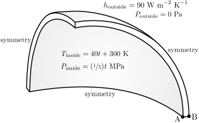
(a) Geometry and loading conditions

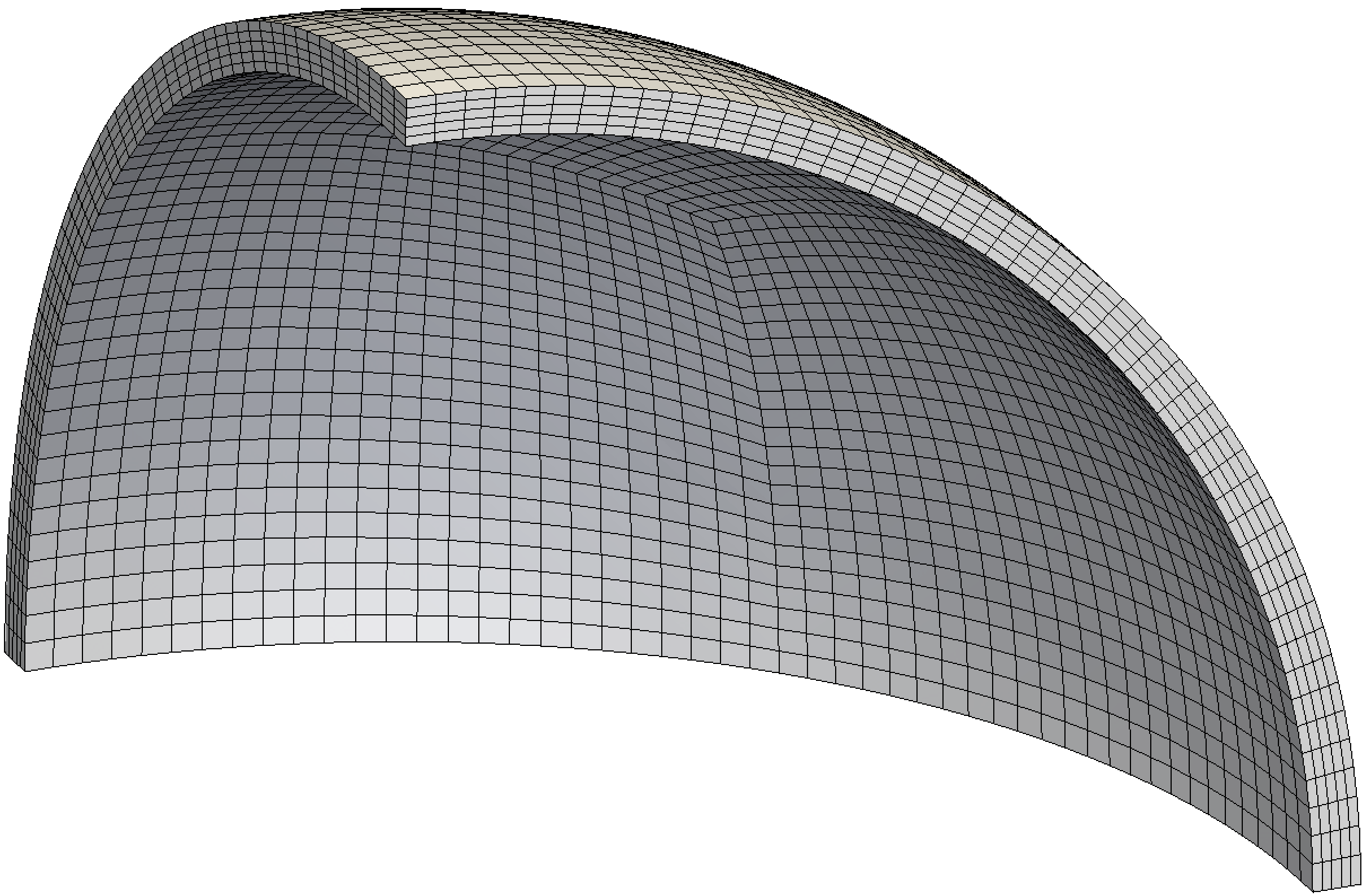
(b) Mesh containing $9~{}375$ cells

Figure 3: Heated spherical pressure vessel: problem geometry, loading conditions and mesh

The one-eighth spherical geometry is shown in Figure 3(a), where the inner radius is 190 m m  and the outer radius is 200 m m . A structured hexahedral mesh has been generated using the OpenFOAM blockMesh mesh utility; in this case, blockMesh from the OpenFOAM-dev fork [89] of OpenFOAM has been used as it allows meshing of spherical surfaces. Four successively refined hexahedral meshes have been employed containing $9~{}375$, $75~{}000$, $600~{}000$ and $4~{}800~{}000$ cells respectively; the coarsest mesh is shown in Figure 3(b).

As indicated in Figure 3(a), the loading conditions consist of a time-varying pressure and temperature on the inside of the sphere:

$$P_{\text{inside}}=\left(\frac{1}{5}\right)t\quad\text{\mathrm{ M }\mathrm{ Pa }}$$

$$T_{\text{inside}}=40t+300\quad\text{\mathrm{ K }}$$ (34)

where $t$ is time, varying from 0 to 5 s . The outer surface is specified as traction free, with a surface convective heat coefficient of $h=90$ W / m ^ 2 K ; the reference atmospheric temperature is assumed to be $T_{\infty}=300$ K . As one-eighth of the geometry is modelled, three symmetry conditions are employed.

The assumed thermo-material properties are given in Table 3, where the stress-free reference temperature is $300$ K .

Young’s modulus	$E$	190 G Pa
Poisson’s ratio	$\nu$	0.305
Density	$\rho$	7750 k g / m ^ 3
Coefficient of thermal expansion	$\alpha$	$9.7\times 10^{-6}$ / K
Specific heat capacity	$C$	486 J / K
Thermal conductivity	$k$	20 W / m K

Table 3: Heated spherical pressure vessel: thermo-mechanical properties

At the initial time, $t=0$ s , the temperature of the domain is 300 K , the displacement is $(0~{}0~{}0)$ m , and the initial velocity is $(0~{}0~{}0)$ m / s . A constant time-step of 1 s  is employed, simulating five time-steps in total, from 0 to 5 s ; the time-step size of 1 s  was selected as it was found to produce time-step independent results on all meshes.

Figure 4 shows the temperature distribution across the wall thickness from point A to point B at $t=5$ s   where the position of points A and B are indicated in Figure 3(a). The predictions are shown for the four meshes; for reference, results are given from Afkar et al. [88] and predictions generated with commercial finite element software Abaqus are shown using the finest mesh; the FE model uses axisymmetric full integration bi-linear elements (Abaqus element code: CAX4T). Little difference can be seen between the predictions on the different meshes, indicating the discretisation error is small in all cases; this is an expected result given the temperature distribution is close to linear.

Figure 4: Heated spherical pressure vessel: temperature distribution across the wall thickness at $t=5$ s

Figure 5(a) shows the von Mises distribution across the wall thickness, from point A to point B, for the four meshes; once again for comparison results are given from Afkar et al. [88] and using the finest mesh with FE software Abaqus. As the mesh density is increased, the predictions can be seen to become mesh independent, with even the coarsest mesh capturing the trend. By examining the error in the von Mises stress prediction at the inner surface, the discretisation error, shown in Figure 5(b), can be seen to reduce at an approximately second error rate i.e. discretisation error reduces by a factor of four when the mesh spacing is halved. The reference solution is approximated using Richardson’s extrapolation [90].

(a) Von Mises stress distribution

(b) Reduction of discretisation error in the von Mises with increasing mesh refinement

Figure 5: Heated spherical pressure vessel: von Mises stress distribution across the wall thickness at $t=5$ s  and the reduction in discretisation error as the cell size is reduced

To illustrate the parallel efficiency of the method, the finest mesh, containing 4.8 million cells, is solved using increasing numbers of CPU cores; the METIS decomposition method [91] has been used to decompose the domain. In the ideal case, the method should scale linearly i.e. relative to the time taken to simulate the case using one CPU core, it should take one tenth of this time using ten CPU cores, one hundredth of the time using 100 CPU cores, and one thousandth of the time using 1000 CPU cores, etc. The time taken to analyse the case using increasing numbers of CPU cores is shown in Figure 6(a); the parallel speedup, defined as $\nicefrac{{T_{\text{core=1}}}}{{T_{\text{core=N}}}}$, is shown in Figure 6(b), where $T_{\text{core=1}}$ is the time taken to simulate the problem using 1 CPU core and $T_{\text{core=N}}$ is the time taken using $N$ CPU cores; in this case $N$ was varied from 6 to 768 CPU cores. As it would have taken an excessive amount of time to solve the problem on one CPU core, the time taken to solve the problem on one CPU core has been approximated as $T_{\text{core=1}}\approx 6\times T_{\text{core=6}}$. The simulation wall-clock times are given for reference in Table 4, where the approximate number of cells per CPU core are indicated. The Fionn supercomputer from the Irish Centre for High-End Computing has been used for all calculations, where each compute node contains two Intel^® Xeon^® (E5-2660 v2 @ 2.20GHz, 25.6 M  of cache) CPUs and 64 GiB of RAM.

In the current parallel efficiency analysis, the total number of cells in the mesh remains constant and the question becomes how many cores should we use to get answer in the shortest time? This corresponds to a so-called strong parallel scalability test, where the total amount of computational work remains constant and the number of CPU cores is increased to try reduce the time required. In contrast, a weak parallel scalability aims to keep the amount of work per CPU core constant, while increasing the number of CPU cores used i.e. for a given amount of time and assuming we are not restricted in the number of CPU cores we can use, how large a problem can we solve?

(a) Simulation time

(b) Parallel speedup

Figure 6: Heated spherical pressure vessel: parallel efficiency for the mesh containing 4.8 million cells

From Figures 6(a) and 6(b), it can be seen that the method scales in an approximately linear fashion up until 384 CPU cores i.e. the solution is attained approximately 384 times faster using 384 CPU cores than using 1 CPU cores. This corresponds to approximately $12~{}500$ cells per CPU core. As the number of CPU cores are increased further to 768, the parallel efficiency drops and in this case attaining the solution using 768 CPU cores is in fact slower than using 384 CPU cores; this can be explained by noting that parallel performance is a competition between computational work done per core versus the amount of information communicated between the cores. As the number of the cores is increased, the amount of work done per core is decreasing while the amount of communication between the cores is increasing; at a certain point, the time taken for communication between the cores becomes significant and increasing the number of cores further can be expected to increase the simulation time.

As a rule of thumb for FV methods in CFD using standard iterative solution methodologies, achieving good parallel efficiency requires approximately $20\times 10^{3}$ to $50\times 10^{3}$ cells per CPU core; in the current case, the noted behaviour was slightly more efficient requiring only $12.5\times 10^{3}$ cells per core, where the solution for the finest mesh was achieved in under half an hour using 384 CPU cores, in comparison to over 25 hours when using 1 CPU core; this is in keeping with previous findings for FV solid mechanics, for example, [10].

Number of CPU cores	Wall-clock time (in h )	Speed-up	Cells per CPU core
1	150.70 (estimated)	-	$4800\times 10^{3}$
6	25.12	6	$800\times 10^{3}$
12	15.01	10.04	$400\times 10^{3}$
24	9.54	15.80	$200\times 10^{3}$
48	4.21	35.77	$100\times 10^{3}$
96	1.70	88.74	$50\times 10^{3}$
192	0.67	224.65	$25\times 10^{3}$
384	0.44	342.50	$12.5\times 10^{3}$
768	0.71	211.18	$6.25\times 10^{3}$

Table 4: Heated spherical pressure vessel: parallel simulation times for the mesh 4.8 million cells

5.2 A 3-D Elastic Punch

In this case, a flat punch with rounded edges is pressed into a flat-topped cylinder. The case has been proposed as a contact mechanics benchmark by the National Agency for Finite Element Methods and Standards (NAFEMS) [92, 93], and has been examined previously a number of times, for example, [94].

The case demonstrates a 3-D quasi-static contact analysis of differing materials; the case and solution is expected to be 2-D axisymmetric but is simulated here as 3-D with symmetries for demonstrative purposes. The problem geometry, shown in Figure 7(a), consists of a cylindrical punch with radius 50 m m  and a 10 m m  filleted edge, in contact with a flat-topped cylinder of 100 m m  radius. The geometry has been created using open-source software FreeCAD [95] and exported in the IGES format to the open-source Gmsh software [96] to create a facetted STL surface file; subsequently, a Cartesian mesh has been created using the OpenFOAM meshing utility cfMesh [97]. Four approximately uniform Cartesian-based meshes of increasing refinement - 4 946, 31 513, 228 026 and 1 789 600 cells - have been employed, where the coarsest mesh is shown in Figure 7(b).

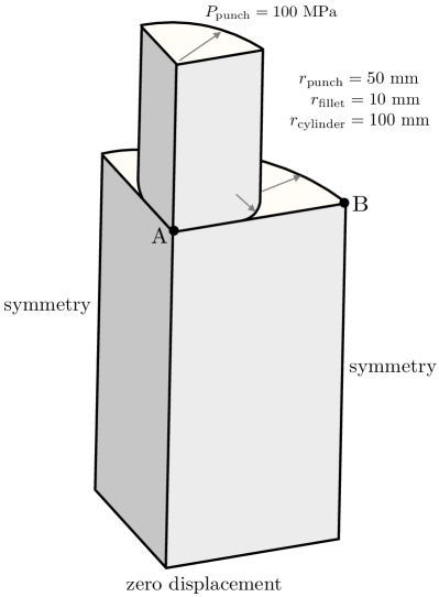
(a) Geometry

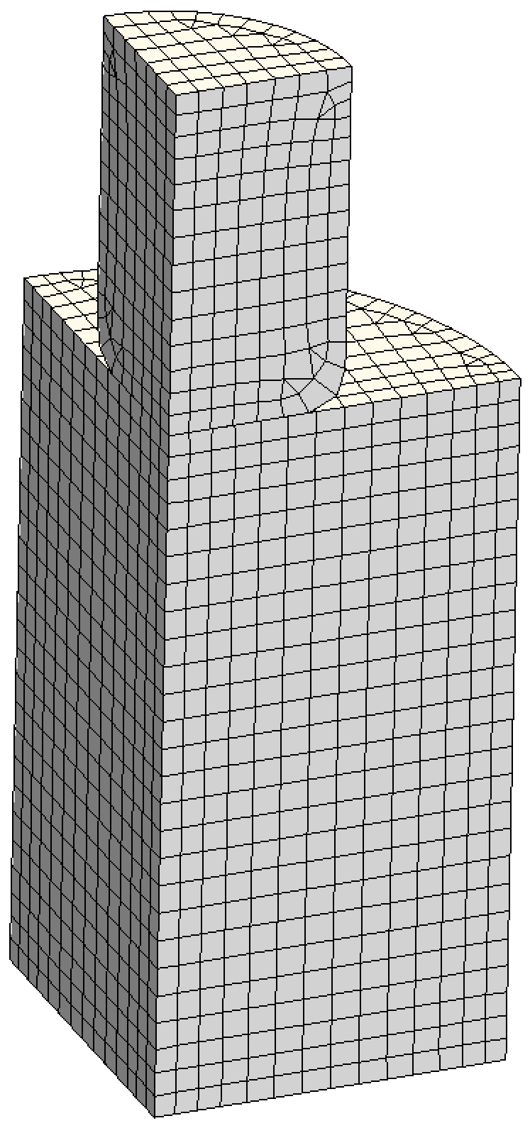
(b) Mesh containing 4 946 cells

Figure 7: A 3-D Elastic Punch: problem geometry and mesh

The punch is assumed to be steel and the cylinder is assumed to be aluminium, where the mechanical properties are given in Table 5; it should be noted that the Poisson’s ratios need not be set the same, and have only been done so here to allow comparison with the NAFEMS results.

Punch
Young’s modulus	$E$	210 G Pa
Poisson’s ratio	$\nu$	0.3
Cylinder
Young’s modulus	$E$	70 G Pa
Poisson’s ratio	$\nu$	0.3

Table 5: A 3-D Elastic Punch: mechanical properties

A pressure of 100 MPa is applied to the upper surface of the punch, and the lower surface of the cylinder is fixed i.e. displacement is zero; in addition, two symmetry plane conditions are employed as indicated in Figure 7(a). To enforce the contact constraint conditions between the punch and cylinder surfaces, a penalty formulation is employed for both the normal and friction models; further details are given previously [15, 11]. The case is solved in one static time-step where inertia and gravity terms are neglected. A linear equation under-relaxation factor of 0.999 is used to ensure convergence; the use of equation (as opposed to field) under-relaxation has been found to be important in contact analyses.

The predicted displacements and stresses are examined on the cylinder surface along a radial line from point A to point B, as shown in Figure 7(a); the predicted axial displacement distribution is shown in Figure 8(a), where the results for the four meshes of increasing refinement are compared with predictions from the NAFEMS benchmark [93]; the reference plots have been digitised using the WebPlotDigitizer software [98]. Figure 8(b) shows the predicted radial displacement distribution, and Figure 9(a) shows the contact pressure distribution. Both displacement and stress predictions can be seen to approach the reference solutions as the mesh is refined.

(a) Axial displacement

(b) Radial displacement

Figure 8: A 3-D Elastic Punch: displacement predictions on the cylinder surface

To examine discretisation error, the axial displacement at point A on the surface of the cylinder is examined for the four meshes; Figure 9(b) shows the discretisation error to reduce from over 20% to less than 1% as the mesh is refined, where the reference displacement is approximated using Richardson’s extrapolation [90].

(a) Von Mises stress distribution

(b) Reduction of discretisation error in the axial displacement at point A with increasing mesh refinement

Figure 9: A 3-D Elastic Punch: contact pressure stress distribution on the cylinder surface and the reduction in discretisation error

5.3 Stress relaxation of a viscoelastic tube

This case consists of a tube constructed from a viscoelastic material, where the inner surface is quickly displaced in the radial direction; the tube relaxes towards steady-state after initially experiencing high wall stresses. A similar case has been examined in the documentation of the commercial finite element software Comsol [99].

The case demonstrates a transient viscoelastic analysis; the case is modelled as 2-D with quarter symmetries, although the solution in this case is expected to be 1-D axisymmetric. Figure 10(a) shows a schematic of the problem geometry, consisting of a long cylindrical tube with inner radius 5 m m  and outer radius 10 m m . A uniform quadrilateral mesh containing $1~{}152$ cells has been generated using OpenFOAM meshing utility blockMesh.

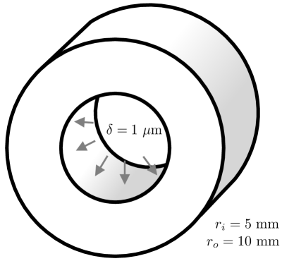
(a) Geometry

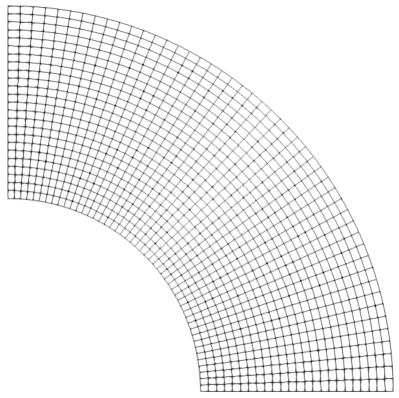
(b) 2-D mesh containing 1 152 cells

Figure 10: Stress relaxation of a viscoelastic tube: problem geometry and mesh

The tube material is assumed to be a viscoelastic polymer and its deviatoric response is represented by a Prony series, whereas its bulk/volumetric response is assumed to be elastic; the mechanical properties are given in Table 6.

Relaxed Young’s modulus	$E_{\infty}$	39.58 G Pa
Poisson’s ratio	$\nu$	0.33
Maxwell Models
Young’s modulus 1	$E_{1}$	2.93 G Pa
Young’s modulus 2	$E_{2}$	5.86 G Pa
Young’s modulus 3	$E_{3}$	6.60 G Pa
Young’s modulus 4	$E_{4}$	18.32 G Pa
Relaxation time 1	$\tau_{1}$	30 s
Relaxation time 2	$\tau_{2}$	300 s
Relaxation time 3	$\tau_{3}$	3 000 s
Relaxation time 4	$\tau_{4}$	12 000 s

Table 6: Stress relaxation of a viscoelastic tube: viscoelastic mechanical properties given in terms of a Prony series

The inner surface of the tube is displaced 1 µ m  in the radial direction; in order to mimic the displacement occurring instantaneously, it is applied within the first time step. The outer surface of the tube is traction free and two symmetry conditions are applied, as indicated in Figure 10(a).

The case is solved over a period of 7 000 s , where inertia and gravity terms are neglected. Four separate time step sizes are examined (700, 350, 175, 87.5 s ) to illustrate the effect of loading increment size on the employed material law integration, where the current method employs the recursive implementation presented by Simo and Hughes [76].

The predicted radial stress on the inner tube surface versus time is examined; the results for the four different time step sizes are shown in Figure 11(a), where results from FE software Abaqus are given for comparison; the Abaqus results have been generated using a time step size of 20 s  to ensure the material integration error is small. Figure 11(b) shows the predicted radial displacement on the inner tube versus time, where the y-axis (displacement) scale does not start from zero to allow the differences to be more clearly seen.

(a) Radial stress

(b) Radial displacement

Figure 11: Stress relaxation of a viscoelastic tube: radial stress and radial displacement predictions across the wall thickness, showing the effect of loading step size

It can be seen that the predicted stresses and displacements are relatively insensitive to the time-step, and as the step size is reduced the predictions are seen to approach the reference solution.

5.4 Perforated Elastoplastic Plate

A perforated plate subjected to tension has been examined a number of times in different forms, for example, [100, 99, 5, 8]. This classic case consists of a thin plate with a circular hole subjected to tension, where in this case, plastic deformation is considered. Owing to the dual symmetries of the problem, one quarter of the plate is modelled and is represented here as plane strain 2-D. The plate has dimensions of $20\times 36$ m m  with a hole of diameter 10 m m , shown schematically in Figure 12(a). Four successively refined structured quadrilateral meshes containing cells 300, 1 200, 4 800 and 19 200 cells have been created using OpenFOAM meshing utility blockMesh; the coarsest mesh, containing 300 cells, is shown in in Figure 12(b).

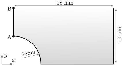
(a) Geometry

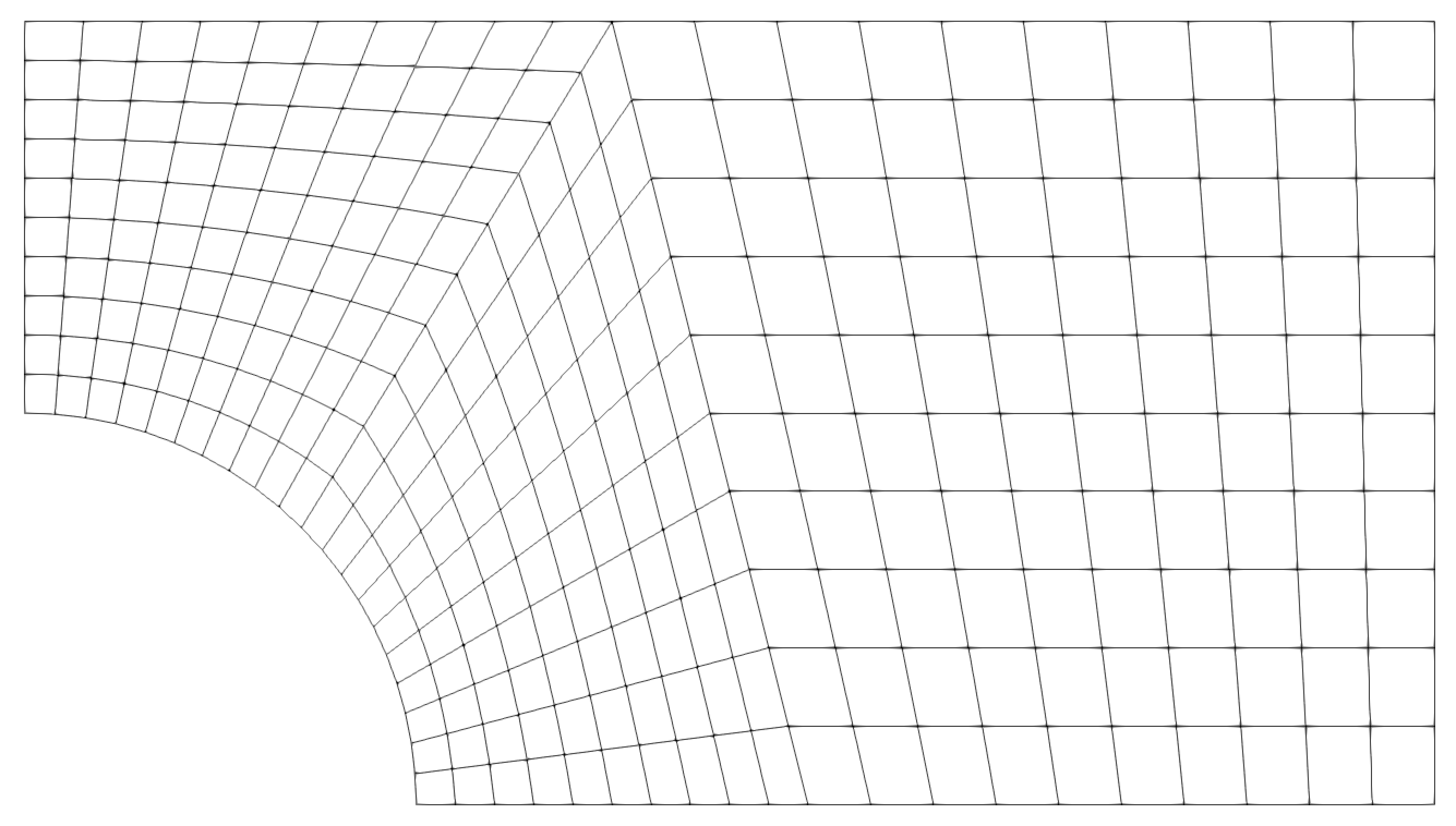
(b) 2-D mesh containing 300 cells

Figure 12: Perforated Elastoplastic Plate: problem geometry and mesh

The aluminium plate material is assumed to be isotropic Hookean elastic with von J₂/Mises yield criterion and isotropic hardening; the mechanical properties are given in Table 7.

Young’s modulus	$E$	70 G Pa
Poisson’s ratio	$\nu$	0.3
Initial yield stress	$\sigma_{Y0}$	243 M Pa
Isotropic hardening modulus	$H$	2.25 G Pa

Table 7: Perforated Elastoplastic Plate: elastoplastic mechanical properties

The right boundary of the plate is loaded with a time-varying normal traction, $T^{n}_{\text{right}}$, that linearly ramps up over the first 10 s  and linearly ramps down from 10 s  to 20 s :

$$T^{n}_{\text{right}}=\begin{cases}13.365t\text{ Pa}&\text{for}\quad 0<t\leq 10\text{ \mathrm{ s }}\\ 13.365(20-t)\text{ Pa}&\text{for}\quad 10<t\leq 20\text{ \mathrm{ s }}\end{cases}$$ (35)

where $t$ is the current time in seconds. Following the approach in [99], the peak value, occurring at $t=10$ s , has been selected so that the mean stress over the section through the hole is 10% above the initial yield stress i.e. $=1.1\times 243\text{ Pa}\times\nicefrac{{(20\text{ mm}-10\text{ mm})}}{{20\text{ mm}}}$. The shear traction on the right boundary is zero. The hole and upper plate boundaries are traction free; symmetry conditions are applied to the left and bottom plate boundaries; 2-D plane strain conditions are assumed. The case is solved over 20 s  in time steps of 0.1 s , where inertia and gravity are neglected.

The predicted $y$ component of displacement at point A on the top rim of the hole is shown in Figure 13(a), where results from FE software Abaqus on the finest mesh are given for comparison. As the mesh is refined, the predictions are seen to become mesh independent, in agreement with the FE results. From Figure 13(b), the residual stress component $\sigma_{xx}$ can be seen along the path A–B at $t=20$ s . As is expected, the region of material near the hole that previously underwent plastic deformation returns to a state of compression upon unloading.

(a) $y$ component of displacement at the upper rim of the hole

(b) Residual stress, $\boldsymbol{\sigma}_{xx}$, along the path A–B at $t=20$ s

Figure 13: Perforated Elastoplastic Plate: displacement and residual stresses predictions

In Figure 14, the regions of predicted active yielding are shown for four time instances; the predictions can be seen to agree closely with the FE results.

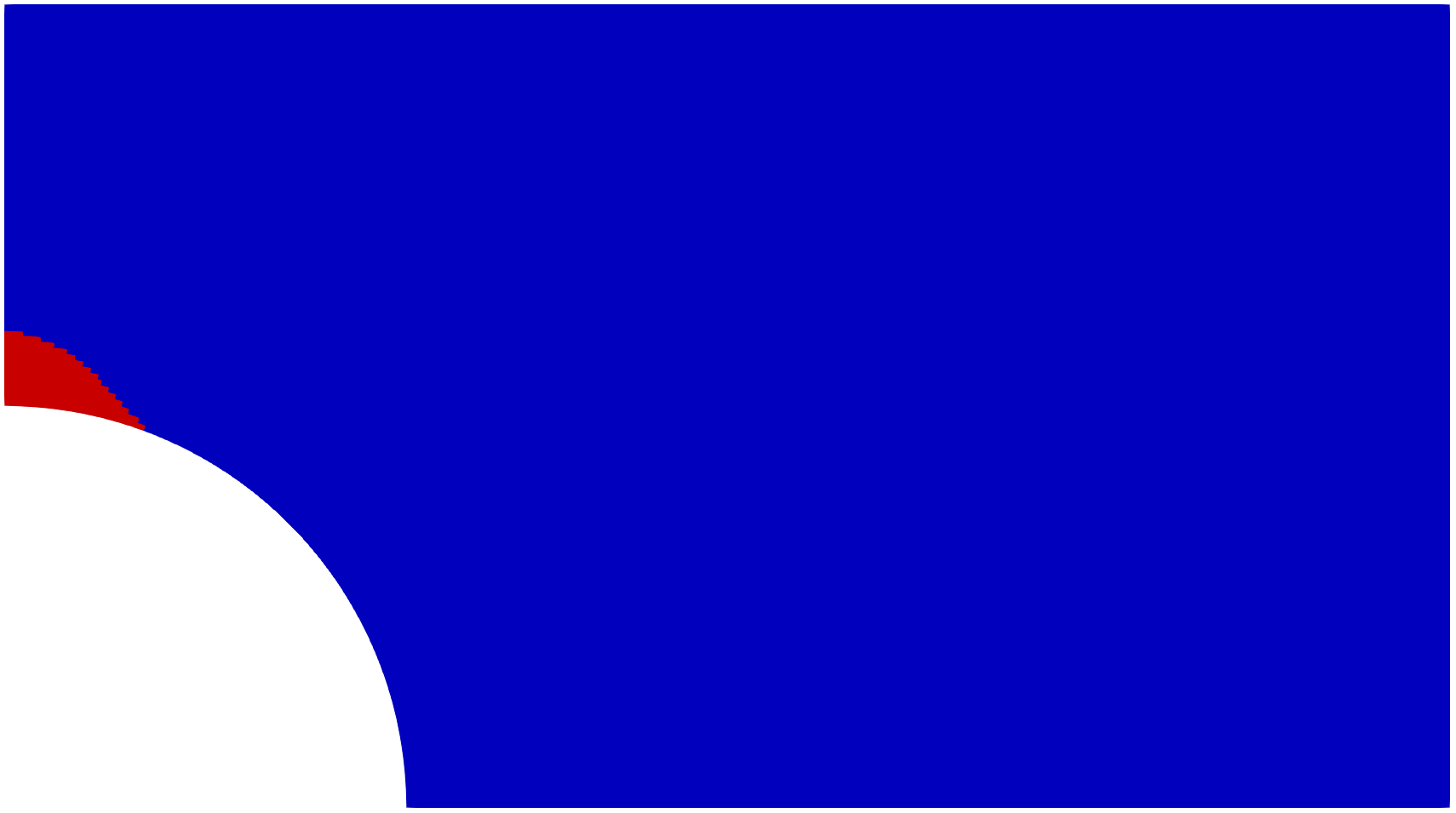
(a) OpenFOAM: $t=7$ s

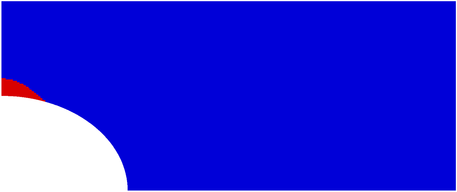
(b) Abaqus FE: $t=7$ s

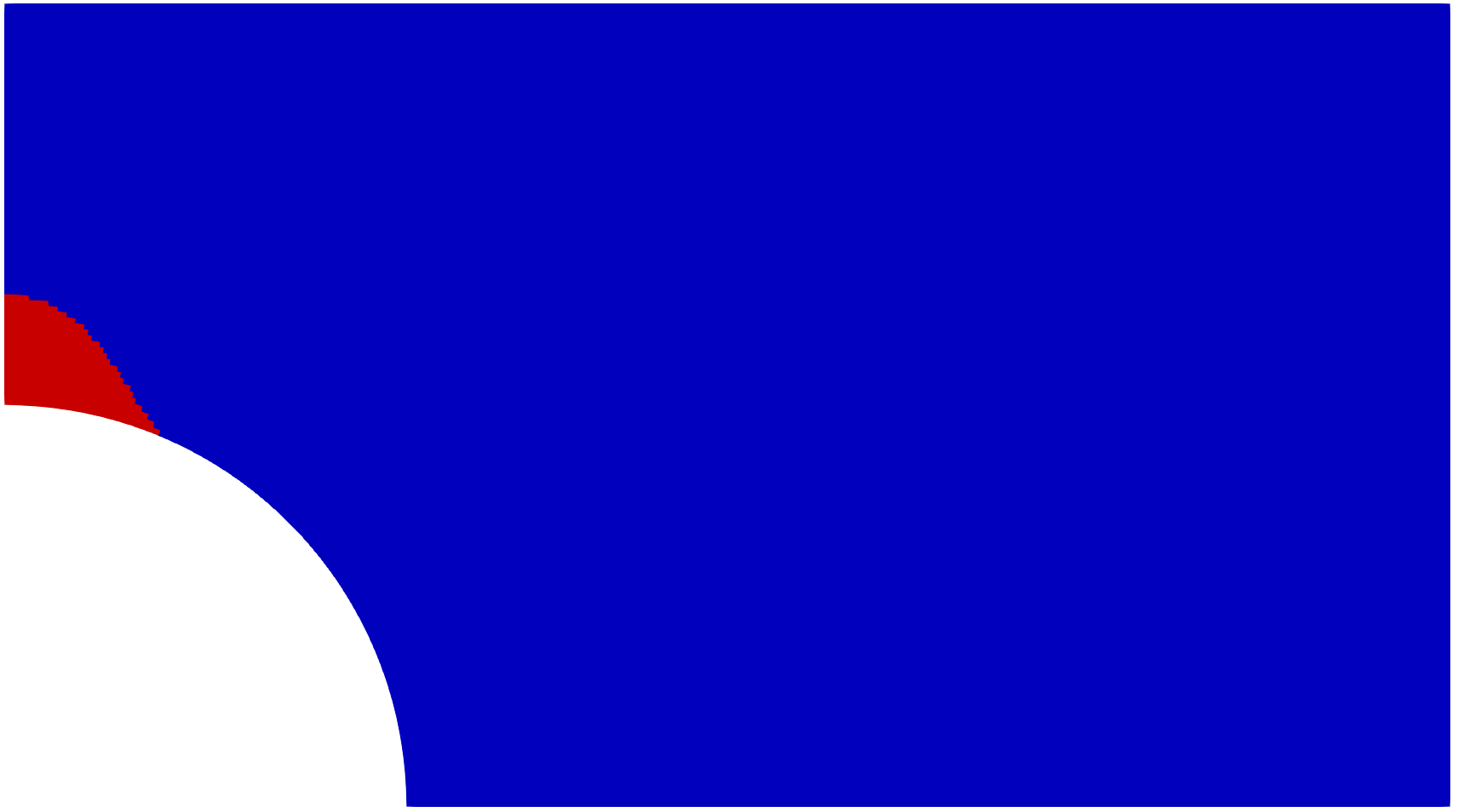
(c) OpenFOAM: $t=8$ s

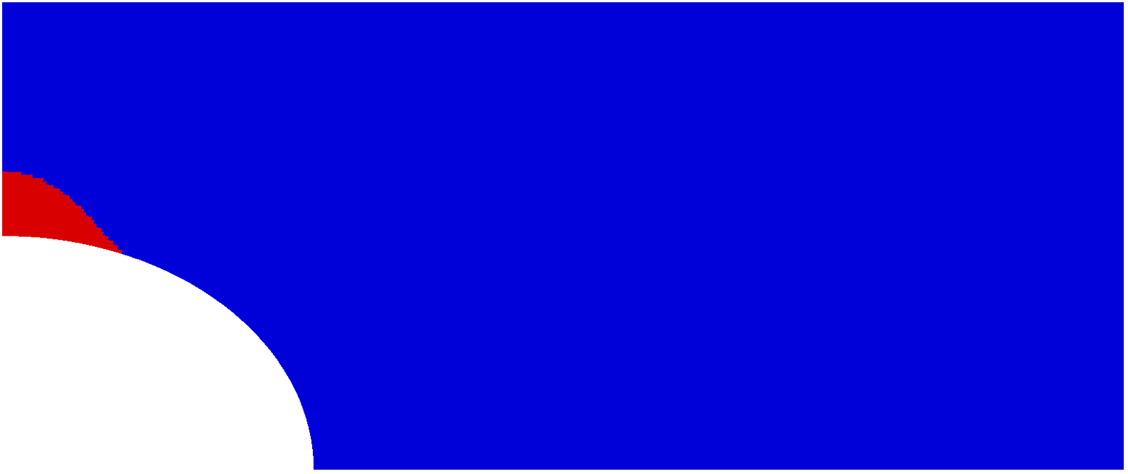
(d) Abaqus FE: $t=8$ s

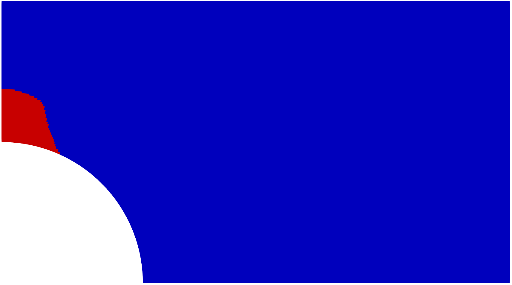
(e) OpenFOAM: $t=9$ s

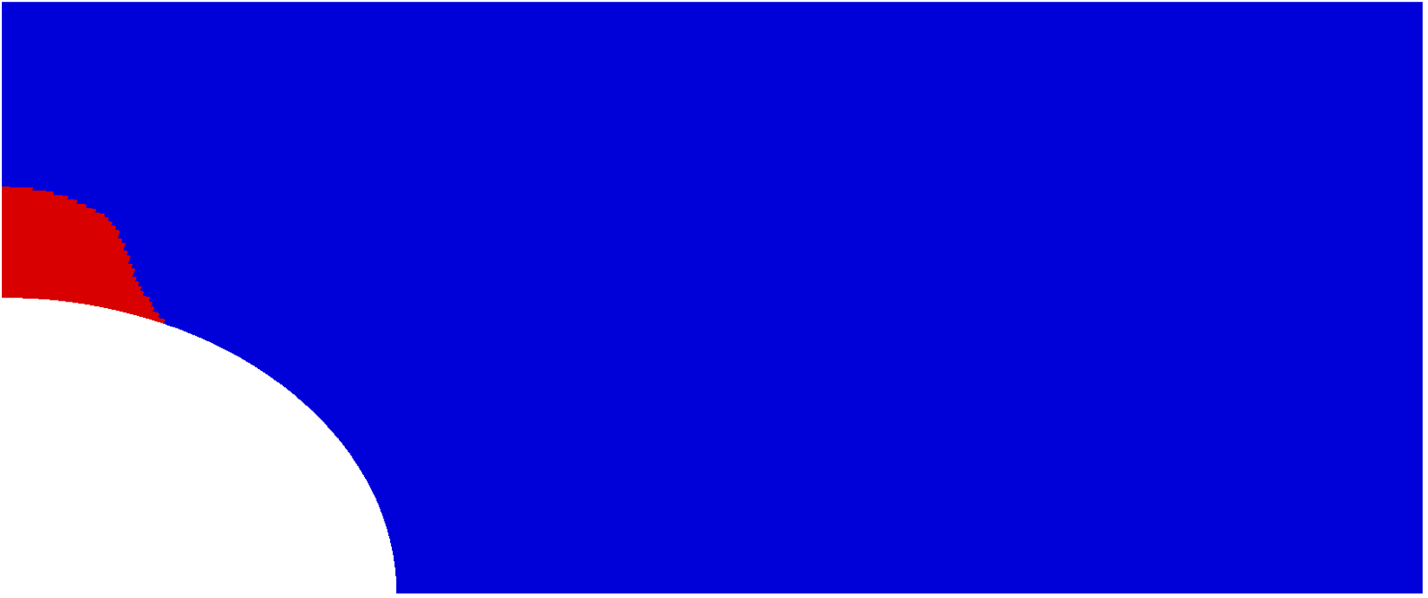
(f) Abaqus FE: $t=9$ s

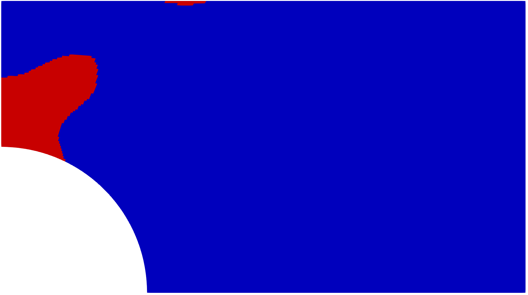
(g) OpenFOAM: $t=10$ s

(h) Abaqus FE: $t=10$ s

Figure 14: Perforated Elastoplastic Plate: regions of predicted active yielding at succesive times

5.5 Micro-Beam in Channel Flow

This case consists of an elastic beam subjected to laminar flow in a channel, and is based on a problem presented in the documentation for the commercial FE software Comsol [99]; it is possible to find a number of similar FSI cases in literature, for example, [101, 34]. The case geometry, shown schematically in Figure 15(a), consists of a solid plate, $50$ µ m  tall and $5$ µ m  wide with a semi-circular top, located $100$ µ m  from the left inlet boundary of a channel, where the channel is $100$ µ m  high and $300$ µ m  long. The geometry for both fluid and solid domain has been created using open-source software Gmsh [96]; the geometry was then exported as a facetted STL surface and subsequently meshed using the OpenFOAM Cartesian meshing utility cfMesh [102]. Figure 15(b) shows the 2-D Cartesian mesh. The fluid domain mesh consists of 3 126 cells, and the solid domain mesh consists of 296 cells.

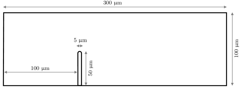
(a) Geometry

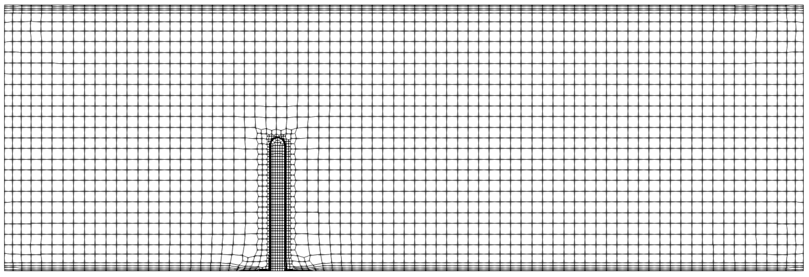
(b) 2-D mesh containing 300 cells

Figure 15: Micro-Beam in Channel Flow: problem geometry and mesh

The physical and mechanical properties of the solid and fluid are given in Table 8; the solid plate is assumed to be a neo-Hookean flexible polymer, where the out-of-plane length is long and hence plane strain conditions are assumed; the fluid is assumed to be incompressible, Newtonian and isothermal.

solid
Density	$\rho_{\text{solid}}$	7850 k g / m ^ 3
Young’s modulus	$E$	700 k Pa
Poisson’s ratio	$\nu$	0.3
fluid
Density	$\rho_{\text{fluid}}$	1000 k g / m ^ 3
Dynamic viscosity	$\eta$	0.001 Pa $\cdot$ s

Table 8: Micro-Beam in Channel Flow: physical and mechanical properties

At the left boundary of the channel, a parabolic inlet velocity is prescribed, where the average flow velocity initially increases rapidly, reaching a peak at 0.215 s   before gradually slowing to a steady-state value of 0.05 m / s . The maximum inlet velocity normal to the left boundary, $U$, is given as:

$$U=\frac{U_{\text{steady}}t^{2}}{\sqrt{(0.04-t^{2})^{2}+(0.1t)^{2}}}$$ (36)

where $t$ is the current time in seconds, and $U_{\text{steady}}$ is the maximum inlet velocity at steady-state i.e. at $t\gg 1$ s . A zero normal gradient of pressure is prescribed at the inlet. The velocity at the upper and lower walls of the channel is set to zero i.e. no slip condition, with a zero normal gradient of pressure. The gauge pressure at the outlet is set to zero, with the normal gradient of velocity also set to zero. The bottom surface of the beam is fixed (zero displacement) and gravity is neglected. At the interface between the fluid and solid regions, continuity of force/traction, displacement and velocity is enforced via Dirichlet-Neumann coupling using Aitken adaptive under-relaxation; more details are found in Tukovič et al.[30, 27, 34].

The model is solved for 1 s  of simulated time, where the time-step is adaptively set to ensure a Courant number of approximately 20.0 in the fluid domain; for the current mesh, this results in an average time-step of approximately 0.2 m s . The fluid is assumed to be water and is solved using the so-called PIMPLE (transient SIMPLE) segregated algorithm and the solid model employs the segregated updated Lagrangian solution procedure and neo-Hookean elastic constitutive law. The material properties given in Table 9.

Fluid
Density	$\rho_{f}$	1000 k g / m ^ 3
Dynamic viscosity	$\eta$	0.001 Pa s
Solid
Density	$\rho_{s}$	7850 k g / m ^ 3
Young’s modulus	$E$	200 k Pa
Poisson’s ratio	$\nu$	0.33

Table 9: Micro-Beam in Channel Flow: material properties

The predicted deformed geometry of the beam at 0.15 s  is shown in Figure 16(b), where the predicted geometry from Comsol [99] is given for comparison.

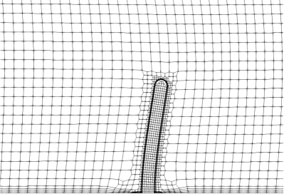
(a) solids4foam

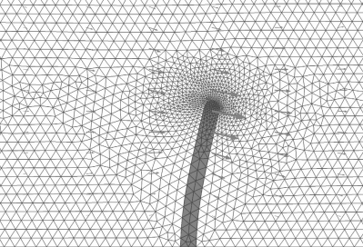
(b) Predictions from Comsol [99]

Figure 16: Micro-Beam in Channel Flow: deformed beam geometry at 0.15 s

The predicted time-varying x component of displacement of the tip of the beam is shown in Figure 17, with results from Comsol [99] given for comparison. The displacement versus time trace from the Comsol documentation has been extracted using the WebPlotDigitizer software [98] and may introduce some errors. Given that a relatively coarse mesh has been used in the Comsol model - there are two triangular elements across the beam thickness - the predicted displacements are generally in agreement. Rather than provide a strict verification benchmark, this test case serves more for demonstration purposes. Stringent benchmarking of the implemented FSI coupling procedure can be found in Tuković et al. [34].

Figure 17: Micro-Beam in Channel Flow: time-varying x-component of the beam tip displacement

The velocity distribution in the channel at 4 s  is shown in Figure 18(a), where once again results from Comsol [99] are given for comparison; contours of equivalent von Mises stress are shown on the solid beam. The results can be seen to be generally in agreement.

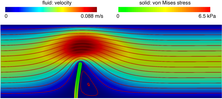
(a) solids4foam

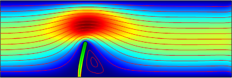
(b) Comsol [99]

Figure 18: Micro-Beam in Channel Flow: velocity distribution in the channel at 4.0 s

6 Summary, Discussion & Conclusions

The current article has presented an open-source toolbox for solid mechanics and FSI simulations based on the FV method, where attention has been given to the design of the use of OOP design principles and code use, comprehension, maintenance, and extension. The toolbox is built on the open-source library OpenFOAM and takes advantage of parallelisation using the method of domain decomposition.

Remark on discretisation in the context of solid mechanics: finite volume vs. finite element

Since the 1970s, the FE method has dominated the field of computational solid mechanics, so much so that the phrase finite element analysis (FEA) has become synonymous with computational solid mechanics. As is evident from the current article alone, alternative methods, such as the finite volume method, have shown similar suitability for tackling a range of CSM problems. The suitability of the FV method for such analyses is not surprising given the close relationship between FE methods and FV methods. Over 20 years ago, Idelsohn and Oñate [103] noted for 1-D diffusion problems that standard continuous Galerkin FE methods are exactly equivalent to the cell-centred FV method, producing the same matrix coefficients. The exact equivalence no longer holds in 3-D and for discretisation of convection/advection terms, but the close relationship is undeniable. A key distinguishing feature of typical FV methods is that they produce strongly conservative discretisations, both locally and globally; this is in contrast to typical FE methods that are weakly conservative. Assuming rigorous mesh sensitivity analyses are performed, the implication of this for CSM problems may be small; however, the development of novel FV discretisation may aid in overcoming shear and volume locking problems, for example, as explored by Haider et al. [23].

As the FV method has developed along the lines of an engineering approach that balances fluxes, this leads to a relatively simple formulation and derivation; in contrast, FE methods take a more mathematical approach, building on the framework of variational and weighted residuals. The FV method applied to CSM comes in many forms, where the presented approach stems from the seminal work of Demirdžić et al. [6] and co-workers in the late 1980s. A large number of alternative forms are found in literature, including fully explicit approaches, vertex-centred methods and so-called parametric formulations [66, 70, 71, 72, 73, 104, 74, 105, 106].

One indisputable disadvantage of the FV method for solid mechanics, relative to the FE method, is that the field of FV CSM is relatively small and somewhat disjointed. This does not, however, take away from the potential of FV to not only equal but to outperform FE methods for some CSM applications; in particular, challenging nonlinear multi-physics problems seem to be prime candidates.

Remark on solution methodologies: segregated vs. coupled

FE methods have typically employed coupled solution methodologies combined with direct linear solvers, where all three displacement components are solved for simultaneously; in contrast, implicit cell-centred FV methods, for example, [7, 11], have used segregated/staggered approaches combined with iterative solvers, where each momentum component equations are temporarily decoupled and solved with outer fixed-point/Picard iterations providing the coupling. Recently, coupled solution approaches have also appeared for FV methods [54, 21]. An advantage of using a segregated approach and iterative solver, for example, the preconditioned conjugate gradient method, is the relative low computer memory requirements, particularly in comparison to using coupled methods with direct solvers, for example, LU decomposition. In the early days of CFD, when computer memory was at a premium, such iterative solution methodologies made large complex 3-D simulations possible. In recent years with the cheap availability of computer memory, this is less of a concern; however, with the movement towards distributed memory computer clusters, iterative solvers once again are becoming attractive with their superior ability to scale in parallel. When combined with multi-grid methods, both algebraic and geometric, the use of iterative solvers for FV (and FE) simulations has the potential to result in highly efficient parallelised solution procedures.

Remark on parallelisation

The procedures presented here directly build on the domain decomposition method of the OpenFOAM library, where the model is partitioned into sub-domains, each of which is solved on a separate CPU core; inter-CPU-core communication provides the necessary coupling information to solve the underlying system of algebraic linear equations. Clearly, efficient parallelisation is predicated on keeping the amount of communication between CPU cores small in comparison to the amount of work done by each CPU core. This means in practice that it would be expected that parallel efficiency drops as the number of cells per CPU core decreases and the number of inter-CPU core cell faces (proportional to inter-core communication) increases. In the presented hot sphere case, this behaviour is evident, where a parallel efficiency of approximately one has been achieved up to 384 CPU cores with 12 500 cells per core, after which the efficiency significantly drops; in fact, the model required more time on 768 CPU cores than on 384.

The parallel efficiency of the presented solvers directly depends on the structure of the OpenFOAM linear equation solvers; however, there are a number of cases where the parallel efficiency is less than that demonstrated here; for example, in contact analyses a neighbour search must be performed to calculate the distances between the master and slave surfaces; this is currently achieved in parallel using so-called global face zones where copies of all the faces and points on the contact boundaries are kept on all processors. In addition, these global face zones are also currently used when passing information between the solid and fluid domains within FSI analyses. In addition, the use of dynamic meshes can result in the number of cells per core becoming unbalanced and consequently load balancing is required to preserve parallel efficiency.

Future directions

The desire for capturing increasingly varied phenomena within multi-physics will lead the future development directions. In particular, this will include the implementation of important solid formulations not currently available within the toolbox, for example, Eigenproblem procedures for buckling and frequency analyses [48], and beam/shell formulations for thin structures. As regards the FV method for beams, plates and shells, suitable approaches have been developed by a number of authors [107, 108, 109, 110]. The so-called finite area method, as developed by [111, 112], for example, would provide a suitable framework for implementation. Separately, the inclusion and exploration of higher-order FV discretisations, for example, approaches recently presented by Demirdžić [64], will also be considered.

In addition to the partitioned FSI approaches presented here, the development of so-called monolithic FSI procedures, where the solid and fluid regions are solved simultaneously, will be considered, and may provide superior stability and efficiency in certain cases. The refactoring of standard fluid models implemented within OpenFOAM will also be performed to link the methods with the solids4foam toolbox, for example, volume-of-fluid multi-phase procedures and block-coupled fluid methods.

Conclusions

An open-source solid mechanics and FSI toolbox is presented, where emphasis has been given to employing effective coding design paradigms. The applicability of the FV-based solvers have been demonstrated on a number of cases, and the methods have been shown to provide a comparable approach to standard FE methods. The toolbox is released as open-source under the GNU Public License [2].

7 Acknowledgements

Financial support is gratefully acknowledged from Bekaert through the University Technology Centre (UTC), and from the Irish Centre for Composites Research (IComp). In addition, the authors wish to acknowledge the DJEI/DES/SFI/HEA Irish Centre for High-End Computing (ICHEC) for the provision of computational facilities and support.

Appendix A Appendix: Mechanical Parameters

$\lambda>0$	first Lamé parameter
$\mu>0$	second Lamé parameter (shear modulus)
$\kappa>0$	bulk modulus
$\boldsymbol{C}_{e}$	fourth order elastic constitutive tensor
$g(t)$	normalised relaxation function
$\gamma_{\infty}\geq 0$	long-term relative modulus
$\gamma_{i}\geq 0$	relative modulus of the ith Maxwell model spring
$N>0$	bulk modulus
$\tau_{i}>0$	relaxation time of the ith Maxwell model spring
$T_{0}$	stress-free reference temperature
$p$	pore-pressure
$\boldsymbol{\epsilon}_{e}$	elastic strain
$\boldsymbol{\epsilon}_{p}$	plastic strain
$\Lambda$	plastic multiplier
$f$	yield function
$\sigma_{Y}$	yield stress/strength
$\epsilon^{eq}_{p}$	equivalent plastic strain
$g$	plastic potential
$\sigma_{1}\geq\sigma_{2}\geq\sigma_{3}$	principal stresses
$\phi$	friction angle
$c$	cohesion strength
$\psi$	dilation angle

Table 10: Mechanical parameters for the linear geometry constitutive laws

Appendix B Appendix: OpenFOAM Implementation of the Linear Geometry Segregated Algorithm

The OpenFOAM implementation of the segregated linear geometry Solid Model class is shown in Listing 1; implicit discretisation operators (finite volume method in OpenFOAM nomenclature) are indicted by fvm:: and explicit operators (finite volume calculus in OpenFOAM nomenclature) are indicated by fvc::.

Listing 1: Code excerpt from the segregated linear geometry class: linGeomSolid

⬇

1// Momentum equation outer loop: fixed-point/Picard iterations

2do

3{

4 // Store displacement field for under-relaxation and residual calculation

5 D.storePrevIter();

6

7 // Discretise the geometrically linear, linear momentum equation in terms

8 // of the unknown total displacement field

9 fvVectorMatrix DEqn

10 (

11 rho*fvm::d2dt2(D)

12 == fvm::laplacian(impKf, D)

13 - fvc::laplacian(impKf, D)

14 + fvc::div(sigma)

15 + rho*g

16 + mechanical().RhieChowCorrection(D, gradD)

17 );

18

19 // Apply under-relaxation to the linear system

20 DEqn.relax(DEqnRelaxFactor);

21

22 // Solve the linear system using a run-time selectable linear

23 // solver, for example, the preconditioned conjugate gradient method

24 solverPerfD = DEqn.solve();

25

26 // Apply under-relaxation to the displacement field

27 D.relax();

28

29 // Update the gradient of displacement field

30 mechanical().grad(D, gradD);

31

32 // Calculate the stress field using a run-time selectable mechanical law

33 mechanical().correct(sigma);

34}

35while (!converged);

Appendix C References