Hunting for Metals Using XQ-100 Legacy Survey Composite Spectra

Abstract

We investigate the NV absorption signal along the line of sight of background quasars, in order to test the robustness of the use of this ion as criterion to select intrinsic (i.e. physically related to the quasar host galaxy) narrow absorption lines (NALs). We build composite spectra from a sample of $\sim$ 1000 CIV absorbers, covering the redshift range 2.55 < z < 4.73, identified in 100 individual sight lines from the XQ-100 Legacy Survey. We detect a statistical significant NV absorption signal only within 5000 km s^-1 of the systemic redshift, z_em. This absorption trough is $\sim$ 15$\sigma$ when only CIV systems with N(CIV) > 10¹⁴ cm^-2 are included in the composite spectrum. This result confirms that NV offers an excellent statistical tool to identify intrinsic systems. We exploit the stacks of 11 different ions to show that the gas in proximity to a quasar exhibits a considerably different ionization state with respect to gas in the transverse direction and intervening gas at large velocity separations from the continuum source. Indeed, we find a dearth of cool gas, as traced by low-ionization species and in particular by MgII, in the proximity of the quasar. We compare our findings with the predictions given by a range of Cloudy ionization models and find that they can be naturally explained by ionization effects of the quasar.

1 INTRODUCTION

Quasar outflows have been increasingly invoked by popular evolution models to regulate both star formation in host galaxies and the accretion of material on to central supermassive black holes (SMBH; e.g. Granato et al., 2004; Di Matteo et al., 2005; Hopkins et al., 2016; Weinberger et al., 2017). A SMBH at the centre of a galaxy can produce a large amount of energy ($\sim$ 10⁶² erg). Even if just a few per cent of the quasar bolometric luminosity were injected into the interstellar medium (ISM) of the host galaxy, it could have a significant impact on the host galaxy evolution (Scannapieco & Oh, 2004; Prochaska & Hennawi, 2009; Hopkins & Elvis, 2010). Such feedback offers a natural explanation for the observed mass correlation between SMBHs and their host galaxy spheroids (e.g., King, 2003; McConnell & Ma, 2013). However, the actual mechanisms of feedback remain highly uncertain.

Outflows are often studied in the rest-frame ultraviolet (UV) via blueshifted narrow absorption lines (NALs) defined by full width at half maximum (FWHM) $\lesssim$ 300 km s^-1. These absorbers are ubiquitously found and detected in all active galactic nuclei (AGN) subclasses (e.g., Crenshaw et al., 1999; Ganguly et al., 2001; Vestergaard, 2003; Misawa et al., 2007). The limitation of NALs is that they arise from a wide range of environments, from high-speed outflows to halo gas to physically unrelated gas or galaxies at large distances from the quasar. Those forming in the proximity of quasars provide valuable tools to study the gaseous environment of quasar host galaxies (e.g. D’Odorico et al., 2004; Wu et al., 2010; Berg et al., 2018).

With the aim of investigating quasar winds, we must select NALs that truly trace outflowing gas cautiously. The outflow/intrinsic origin of individual NALs can be inferred from: i) time variability of line profiles, ii) absorption profiles significantly broader and smoother compared with the thermal line widths, iii) high space densities measured directly from excited-state fine-structure lines, iv) partial coverage of the background emission source measured via resolved, optically thick lines with too-shallow absorption troughs, v) higher ionization states than intervening absorbers. Nonetheless, NALs can still be connected to the quasar host galaxy without exhibiting such properties (Hamann et al., 1997).

Previous works have shown that, among the highly-ionized absorption species commonly used to identify outflows (e.g. CIV$\lambda\lambda$1548,1550; SiIV$\lambda\lambda$1393,1402; NV$\lambda\lambda$1238,1242; OVI$\lambda\lambda$1031,1037), NV is detected with the lowest frequency, but with the highest intrinsic fraction. Misawa et al. (2007) derived an intrinsic fraction of 75 per cent for NV NALs, through partial coverage and line locking methods. Ganguly et al. (2013), using the same techniques, found a value of 29-56 per cent and suggested using this ion in building large catalogs of intrinsic NALs with lower resolution and/or lower signal-to-noise ratio (S/N) data.

In Perrotta et al. (2016, hereafter P16) we used the spectra of 100 quasars at emission redshift z_em = 3.5 - 4.72 to build a large, relatively unbiased, sample of NALs and study their physical properties statistically. The spectra have been obtained with the echelle spectrograph X-shooter (Vernet et al., 2011) on the European Southern Observatory (ESO) Very Large Telescope (VLT) in the context of the XQ-100 Legacy Survey (López et al., 2016). P16 showed that NV is a key line to study the effects of the quasar ionization field, offering an excellent statistical tool for identifying outflow/intrinsic candidate NALs. Indeed, most of the NV systems in our sample exhibit distinctive signatures of their intrinsic nature with respect to intervening NALs (described above), and NV/CIV column density ratios larger than 1 (see Fechner & Richter, 2009).

The large number of Ly$\alpha$ lines characterizing the forest in the spectra of quasars at z_em = 3.5 - 4.72 prevents us in P16 from searching for individual NV lines at large velocity offsets (we could reliably identify NV only within 5000 km s^-1 of z_em). Most of the Ly$\alpha$ forest is associated with moderate overdensities and traces filamentary structure on large scales, but some strong forest absorbers along with Lyman-limit systems (LLSs, N(HI) $\geq$ 10^17.2 cm^-2) and damped Lyman alpha absorptions (DLAs, N(HI) $\geq$ 10^20.3 cm^-2), are thought to be associated with galaxies and the circumgalactic medium (CGM; e.g. Faucher-Giguère & Kereš, 2011; Fumagalli et al., 2011). Therefore, intervening metals associated with Ly$\alpha$ absorbers can probe different environments: from the ISM to the outer regions of galaxies (the CGM) far from the quasar to the more diffuse intergalactic medium (IGM).

In this work, we apply the stacking technique to the XQ-100 spectra to look for NV at large velocity separations from z_em. Indeed, when an ensemble of independent sight lines is stacked to produce a composite spectrum, the numerous stochastic HI absorptions average together and the resulting spectrum is flat, revealing any strong metal signal buried within the Ly$\alpha$ forest. These measurements will complement our previous study on NV and test the robustness of our claim on the use of NV as a criterion to select intrinsic NALs.

The work is organized as follows: Section 2 describes our methodology for identifying NALs; Section 3 collects the details of the procedure followed to build the stacking spectra. Our results are presented in Section 4 and Section 5 discusses the original findings of our study. Our conclusions are summarized in Section 6.

We adopt a $\Lambda$CDM cosmology throughout this manuscript, with $\rm\Omega_{M}$ = 0.315, $\Omega_{\Lambda}$ = 0.685, and H₀ = 67.3 km s^-1 Mpc^-1 (Planck Collaboration et al., 2014).

2 DATA

To carry out the study of NV absorption systems, we start from the CIV sample that we collected in P16. The CIV NALs are identified in quasar spectra from the XQ-100 Legacy Survey (López et al., 2016). The most common metal transition found in quasar spectra is CIV. Roughly half of the Ly$\alpha$ forest with N(HI) $\geq$ 10^14.5 cm^-2 is CIV-enriched at z $\sim$ 3 (Cowie et al., 1995; Songaila, 1998). CIV enrichment has even been suggested at lower N(HI) (Songaila, 1998; Ellison et al., 2000; Schaye et al., 2003; D’Odorico et al., 2016). This is the main reason why we start our analysis from a sample of CIV absorbers, as well as a better alignment of the CIV systems with other metal lines with respect to Ly$\alpha$ absorbers (Kim et al., 2016).

In P16, we identify almost one thousand CIV doublets (1548.204, 1550.78 Å) covering the redshift range 2.55 < z < 4.73. The catalogue is produced with the goal of mapping the incidence of NALs in the quasar rest-frame velocity space. Our study includes any CIV absorber outside the Ly$\alpha$ forest in each spectrum (up to $\sim$ 71,580 km s^-1 from z_em). We refer to systems occurring at less than 5000 km s^-1 from the systemic redshift of the quasar as associated absorption lines (AALs).

We refer to P16 for a complete description of the identification and measurement of equivalent width (EW) and column density (N) of CIV absorbers.

The absorber velocity (v_abs) with respect to the quasar systemic redshifts is computed by the relativistic Doppler formula,

$$\\ \\ \\ \ \rm\beta\equiv\frac{v_{abs}}{c}=\frac{(1+z_{em})^{2}-(1+z_{abs})^{2}}{(1+z_{em})^{2}+(1+z_{abs})^{2}}$$ (1)

where z_em and z_abs are the emission redshift of the quasar and the absorption redshift of the NAL, respectively, and c is the speed of light.

Our final sample includes 986 CIV doublets with $-$1000 < v_abs < 71,580 km s^-1 and equivalent widths 0.015 Å < EW < 2.00 Å.

Thanks to the high S/N and wavelength extent of our spectra, we are able to search for other common ions (NV, SiIV, CII, etc) at the same redshifts of the detected CIV absorbers. However, contamination by the Ly$\alpha$ forest prevents us from investigating the same velocity range for all the ions. In particular, our final sample consists of 46 NV absorbers with column density down to Log N(NV) $\sim$ 12.8 cm^-2, corresponding to a probability of 38 per cent to find a NV at the same z_abs of a given CIV NAL with v_abs < 5000 km s^-1. 55 per cent of NV systems have column densities larger than Log N(NV) > 14 cm^-2 and 85 per cent have values larger than Log N(NV) > 13.5 cm^-2. Furthermore, 68 per cent of the NV NALs have column densities larger than the corresponding CIV.

3 STACKING PROCEDURE

We adopt the stacking technique to explore the presence of NV signal in the Ly$\alpha$ forest associated with the CIV absorbers described in the previous section. The first step to produce the stacked spectrum is the continuum normalization of all the XQ-100 quasar spectra. The continuum placement in the Ly$\alpha$ forest is highly subjective, due to few portions of the spectrum free from absorption (e.g. Kirkman et al., 2005). The continuum is particularly difficult to identify at the position of DLAs. The estimate of the continuum level is done manually by selecting points along the quasar continuum free of absorption (by eye) as knots for a cubic spline. For all sightlines, the continuum placement is inspected visually and adjusted such that the final fit resides within the variations of regions with clean continuum. Then, the flux and error arrays are continuum-normalized. The accuracy of the fits is as good as or better than the S/N of these clean continuum regions (see López et al., 2016 for a detailed description of the adopted procedure).

We follow the subsequent scheme for the construction of the average spectrum.

(i) For each of the 986 CIV systems identified in P16, we consider the position of the velocity component with the highest optical depth of the absorption profile as the redshift of the system, z_abs, around which we select the spectrum region to stack. For completeness, we will show how the results change calculating the barycentre position of the system weighting the wavelengths with the optical depth of the line profile (see Sec. 4.4).

(ii) We use the CIV centre, z_abs, to select the region of the spectrum where the corresponding NV doublet should be located. Specifically, we select a region of $\pm$ 1000 km s^-1 around the expected position of the NV centre (for both doublet components; i.e. NV$\lambda$1238   and NV$\lambda$1242).

(iii) Each selected region is shifted to the corresponding z_abs rest-frame.

(iv) We generate a rest-frame wavelength array with fixed wavelength step $\Delta\lambda$. The step value is set to be slightly larger than the pixel size of the UV spectra. The visible arm of X-shooter has a mean resolution of $\lambda$/$\Delta\lambda$ = 8800, while in the UV it goes down to $\sim$ 5000. Thus, a region with the same extent is sampled with a larger number of pixels in the visible than in the UV region of the spectrum.

(v) For each selected spectral region, we compute the contribution of each pixel to the cells of the final grid.

(vi) All the flux values in each cell of the final grid are then averaged to produce the stacked spectrum.

(vii) Uncertainties on the observed stack are estimated through the bootstrap resampling technique. From a given number, N, of rest-frame spectral regions, we consider the first pixel of each region as the element of an array. We randomly sample from this array, allowing for replacement, to form a new sample (called bootstrap sample) that is also of size N. This process is repeated a large number of times (e.g. 1000 times), and for each of these bootstrap samples we compute its mean. We now have a histogram of bootstrap means. This provides an estimate of the shape of the distribution of the mean. The measured standard deviation of this distribution is the error we associate with the first pixel of the stacked spectrum. Then, the method is applied to all the pixels of the rest-frame spectral regions to be stacked.

Our study is not so sensitive to the continuum placement because we do the analysis relative to the average IGM opacity, without the goal of measuring the opacity.

For each sightline, we mask out the regions that have clear strong absorption features (i.e. Lyman breaks, sub-DLAs with N(HI) $\sim$ 10^19-20.3 cm^-2 and DLAs) when they coincide with those to be stacked. In particular, we take advantage of the DLA identification done by Sánchez-Ramírez et al. (2016). We define the extremes of the DLA absorption at the wavelengths where the wings of the DLA again match the level of the continuum to within the values of the flux error array.

We exclude 77 NV regions because they completely or partially overlap with Lyman breaks or DLA and sub-DLA absorptions. Our final sample consists of 909 NV selected regions, the centre of which is within $-$1000 < v_abs < 71,580 km s^-1 of z_em. We extend the explored velocity range to $-$1000 km s^-1 to take uncertainties in the quasar systemic redshift into account (López et al., 2016) and to consider possible inflows.

This method is powerful in detecting even weak absorption features in the Ly$\alpha$ forest, where confusion noise from forest absorption lines makes it very difficult to identify individual metal lines reliably. However, NV is one of the most rarely detected ions in optically thin (i.e. N(HI) $\lesssim$ 10¹⁷ cm^-2) intergalactic absorption systems and its signal is diluted if we stack regions selected within any velocity shift from z_em up to 71,580 km s^-1.

4 RESULTS

The following sections collect the results of the search for metal absorptions corresponding to CIV clouds with 10^11.5 < N(CIV) < 10^16.5 cm^-2 (see P16). We first investigate the presence of a NV signal as a function of the velocity shift from the quasar to test the nature of NV. Then, we examine many other lower and higher ionization species. The main goal is to characterize the ionization state of the gas both close and far from the continuum source.

4.1 NV Absorption

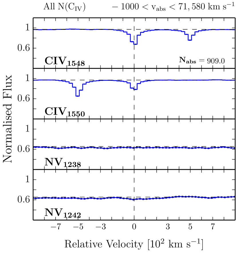
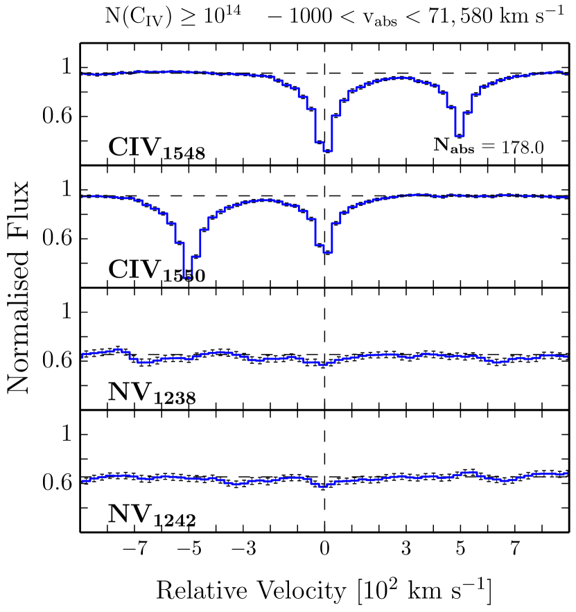
Figure 1: Left: average absorption line spectra for CIV and NV, selected within any velocity separation from z_em. $\rm N_{abs}$ indicates the number of absorbers considered to build the stacked spectrum. Right: same as for the left panels, but in this case only regions corresponding to the strongest CIV NALs (i.e. N(CIV) $\geq$ 10¹⁴ cm^-2) are included in the stack. Error bars are 1$\sigma$ and are estimated by bootstrapping the data using 1000 realizations.

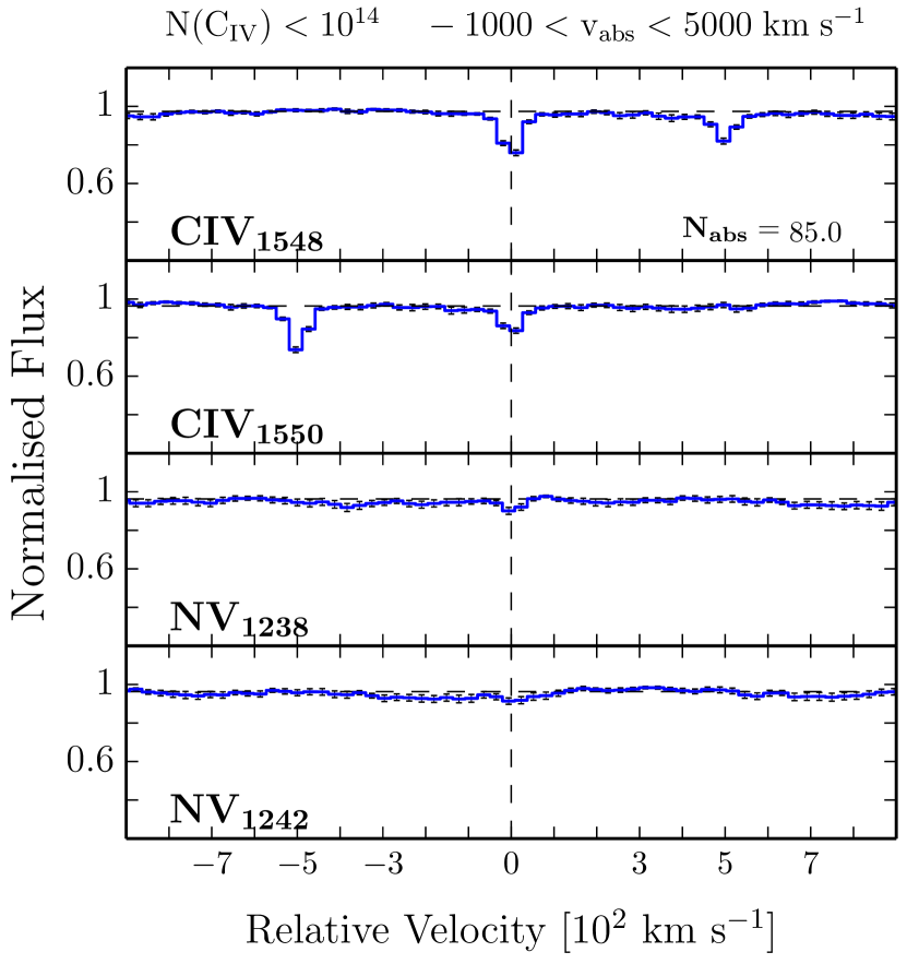
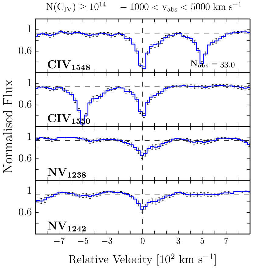
Figure 2: Left: average absorption line spectra for CIV and NV selected within 5000 km s^-1 of z_em. Only regions corresponding to CIV NALs with N(CIV) < 10¹⁴ cm^-2 are included in the stack. $\rm N_{abs}$ indicates the number of absorbers considered to build the stacked spectrum. Right: same as for the left panels, but in this case N(CIV)$\geq$ 10¹⁴ cm^-2 is considered as threshold for the stacking. Error bars are 1$\sigma$ and are estimated by bootstrapping the data using 1000 realizations.

The left panel of Fig. 1 shows the results for CIV and NV absorbers obtained by stacking the whole sample of sight lines. The zero velocity point, v = 0 km s^-1, represents the z_abs of the deepest component of the corresponding CIV system. The average spectrum appears quite flat for both components of the NV doublet, as expected in absence of a strong signal, due to the stochastic nature of the Ly$\alpha$ forest. The continuum level is decreased to a value below 1 due to the cumulative effect of the Ly$\alpha$ forest absorption.

The right panel of Fig. 1 exhibits the CIV and NV composite spectra derived from the stacking of the regions corresponding to CIV NALs with N(CIV) $\geq$ 10¹⁴ cm^-2. This column density threshold matches the value we use in P16 to distinguish between weak and strong CIV systems. Selecting the strongest systems in the sample, we see only a small hint of coherent absorption features in the profile of the two NV doublet components. Fig. 1 combines all of the NALs regardless of velocity shift. In the following, we investigate the presence of a NV signal as a function of the velocity separation from the quasar to understand when it becomes significant. To this end, we produce NV composite spectra in bins of velocity offset from z_em.

Fig. 2 shows the stacked spectra of CIV and NV absorbers with $-$1000 < v_abs < 5000 km s^-1 and as a function of the corresponding N(CIV). In particular, in the left panels the stacked regions are selected so that N(CIV) < 10¹⁴ cm^-2, while in the right ones N(CIV) $\geq$ 10¹⁴ cm^-2. The first column density threshold chosen for the stacking produces a hint of coherent absorption in the profile of both the NV components (left panels). The signal of the absorption line is weak, but represents a 4 $\sigma$ detection. The NV composite spectrum shows the NV lines clearly present at > 15$\sigma$ confidence once only the regions corresponding to the strongest CIV are selected to be stacked (right panels). We note that both NV lines display the same kinematic profile and they also match those of the corresponding CIV NAL.

Table 1: Probability that an individual CIV NAL within 5000 km s^-1 of z_em, shows a NV absorber at the same absorption redshift, as a function of its column density.

	Number of CIV a	CIV with NV b
all	122	38%
Log N(CIV) $\geq$ 14.3	25	72%
Log N(CIV) $\geq$ 14	42	55%
Log N(CIV) $\geq$ 13.5	85	44%
Log N(CIV) < 14.3	97	29%
Log N(CIV) < 14	80	29%

^a Number of CIV NALs with v_abs< 5000 km s^-1 and with column density in the selected range
^b Fraction of CIV NALs with a NV absorber at the same absorption redshift. Detection limit on NV is Log N(NV) $\sim$ 12.8 cm^-2

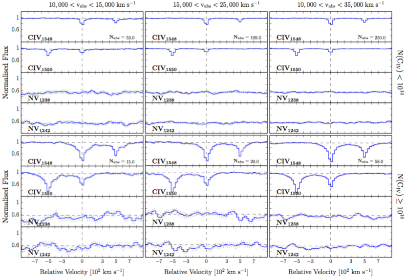
Figure 3: Top panels: the average absorption line spectra produced selecting only CIV systems with N(CIV)$\leq$ 10¹⁴ cm^-2 are shown in different bin size of velocity offset from the z_em. Bottom panels: same as for the top panels, but with a different column density threshold, N(CIV)$\geq$ 10¹⁴ cm^-2.

The associated region is the only spectral window in which we are able to identify individual NV NALs. The number of CIV doublets within 5000 km s^-1 of z_em as a function of the column density is reported in Tab. 1, as well as, the fraction of CIV showing associated NV. The stronger the CIV column density, the higher the probability of selecting systems with NV at the same redshift. This trend is not due to a detection bias affecting the identification of NV NALs at low column densities. Indeed, the high and uniform S/N of the XQ-100 spectra allows us to identify NV systems reliably down to Log N(NV) $\sim$ 12.8 cm^-2 (see P16). In addition, associated NV NALs are preferentially stronger than the corresponding CIV (Fechner & Richter, 2009). However, we adopt N(CIV) = 10¹⁴ cm^-2 as the column density threshold to distinguish between weak and strong systems. This restriction is motivated by the requirement to have a minimum number of systems within a given velocity separation from z_em to build the composite spectrum. This is crucial, especially when we investigate large velocity offsets from z_em, where the number density of CIV NALs exhibits a clear drop with respect to the excess of lines found in proximity to the quasar (see P16). Moreover, Fechner & Richter (2009) have shown that intervening NV systems are systematically weaker than the associated ones: no intervening NV system with N(NV) $\geq$ 10¹⁴ cm^-2 has been detected. It is therefore very important to explore the regime of weak lines.

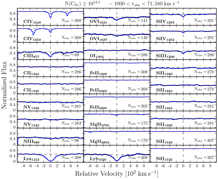
Figure 13: Composite spectra for the ions studied in this work, based on the CIV systems with N(CIV)$\geq$ 10^13.5 cm^-2 and 15,000 < v_abs< 71,580 km s^-1. CIV DLAs are excluded by the stacking. Every panel reports the number of absorbers considered to build the stacked spectrum. The error bars are 1$\sigma$ and are estimated by bootstrapping the data using 1000 realizations. This example demonstrates that the stacking technique applied to the XQ-100 spectra can succeed in detecting absorption lines in the Ly$\alpha$ forest.

To investigate the NV signal beyond the associated region, we build the NV composite spectra in bins of 5000 km s^-1 up to 71,580 km s^-1 from z_em both for weak and strong CIV systems. In particular, Fig. 3 (left column) shows the results for CIV and NV absorbers with 10,000 < v_abs < 15,000 km s^-1. The stacked spectra produced selecting only CIV systems with N(CIV) $\leq$ 10¹⁴ cm^-2 are presented in the top panel, while in the bottom one only CIV systems with N(CIV) $\geq$ 10¹⁴ cm^-2 are considered. In both case, there is no imprint of any significant coherent absorption feature in the profile of the two NV doublet components. We show just one of the many 5000 km s^-1 velocity bins studied, because they all exhibit the same behavior. Fig. 13 in the Appendix demonstrates that the stacking technique applied to the XQ-100 spectra is actually able to detect absorption lines in the Ly$\alpha$ forest.

We then consider larger velocity bins, in order to increase any possible signal of intervening NV absorbers. This is particularly important for the strong systems, which are much rarer at large separations from the quasar (see P16). The stacked spectra produced selecting only CIV systems with 15,000 < v_abs < 25,000 km s^-1 (10,000 < v_abs < 35,000 km s^-1) are presented in the middle column of Fig. 3 (right column of Fig. 3).

The absence of statistical significant intervening NV absorption is a common feature independently of the parameters (N(CIV ) and v_abs) selected as threshold of the stacking. The mean rest frame EW upper limit found for the NV absorption line in the different velocity bins explored is $\sim$ 0.03 Å. This finding strongly suggests that a proximity of 5000 km s^-1 from the quasar is required for NV to be detected.

4.2 Other metal species

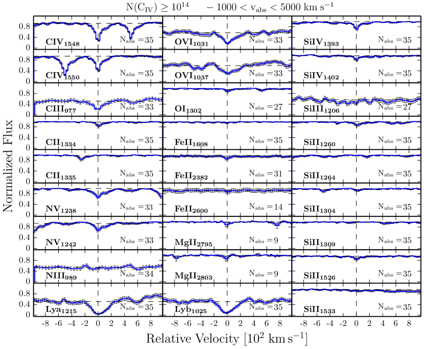
Figure 4: Composite spectra for the ions studied in this work, based on the CIV systems with N(CIV) $\geq$ 10¹⁴ cm^-2 and $-$1000 < v_abs < 5000 km s^-1. Every panel reports the number of absorbers considered to build the stacked spectrum. N_abs is not the same for all the ion species, because each one undergoes a different masking for DLA, sub-DLA and Lyman breaks. The error bars are 1$\sigma$ and are estimated by bootstrapping the data using 1000 realizations. We include MgII and FeII $\lambda$ 2600 lines despite they both suffer of poor statistics.

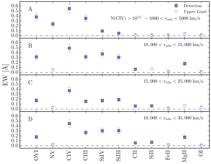
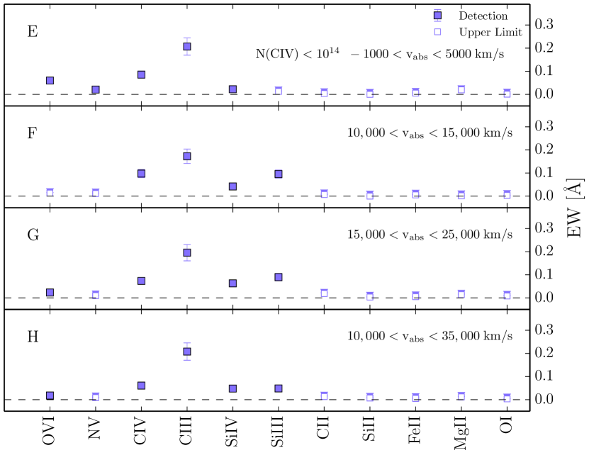
Figure 5: Left: equivalent widths of metal species measured in order of decreasing ionization potential for composite spectra based on the CIV systems with N(CIV)$\geq$ 10¹⁴ cm^-2. Each panel displays an increasing velocity offset from z_em and bin size, going from top to bottom. CIV DLAs have been excluded form the stacking. Right: same as for the left panels, but in this case CIV systems with N(CIV)< 10¹⁴ cm^-2 are included in the stack. The EW refers only to the strongest member of the doublets. Error bars are 1$\sigma$ and are estimated by bootstrapping the data using 1000 realizations.

Besides the stacked spectra to detect NV absorptions, we have computed with the same technique the stacked spectra for the following transitions associated with the sample of detected CIV lines: Ly$\alpha$ $\lambda$1215.67 Å, Ly-$\beta$ $\lambda$1025.72 Å, CIII $\lambda$977.02 Å, CII $\lambda$1334.53 Å, OI $\lambda$1302.16 Å, SiIII $\lambda$1206.50 Å, SiII $\lambda$1260.42, 1304.37, 1526.70 Å, FeII $\lambda$ 2382.76 Å, absorption and SiIV $\lambda\lambda$1393.76, 1402.77 Å, OVI $\lambda\lambda$1031.92, 1037.61 Å and MgII $\lambda\lambda$2796.35, 2803 Å doublet absorption.

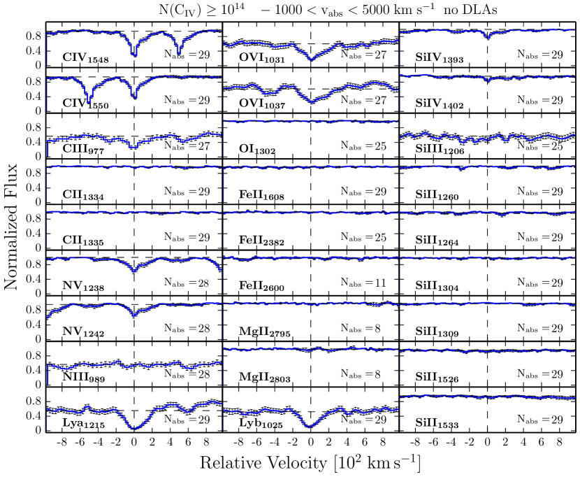
Figure 11: Composite spectra for the ions studied in this work, based on the CIV systems with N(CIV)$\geq$ 10¹⁴ cm^-2 and -1000 <v_abs< 5000 km s^-1. CIV DLAs are excluded from the stacking. Every panel reports the number of absorbers considered to build the stacked spectrum. The error bars are 1$\sigma$ and are estimated by bootstrapping the data using 1000 realizations.

The composite spectrum based on the CIV systems with N(CIV) $\geq$ 10¹⁴ cm^-2 and $-$1000 < v_abs < 5000 km s^-1 is shown in Fig. 4. Based on ionization arguments, we would expect that CIV NALs showing associated ions like NV or OVI ought not to have low ionization transitions. To remove the effects of DLAs on our investigation, we exclude all CIV associated with DLAs (Sánchez-Ramírez et al., 2016) from the stacking. As a consequence, we do not see any significant evidence of absorption trough in the spectra of CII, MgII, SiII, FeII and OI (see Fig. 11). This result is expected, since we have already measured a CII covering fraction of 10 per cent for absorbers with v_abs < 10,000 km s^-1 along the line of sight (P16), in contrast with what is observed in the transverse direction (Prochaska et al., 2014). This finding seems to be confirmed by the absence of a strong MgII signal in the proximity of the quasar. We will come back to this point in Section 4.3.

To quantify the detections clearly present in the composite spectrum, we measure the equivalent widths of the absorption lines. The continuum is first established by fitting a cubic spline function to the spectral regions free of apparent absorption lines. Then, the rest-frame equivalent width is measured as described in Section 2. We present our metal-line equivalent width measurements in Fig. 5. For those lines that are not detected at over 3 $\sigma$ significance level, we give the 3$\sigma$ upper limits on their equivalent widths.

The left panels of Fig. 5 show the equivalent widths derived for composite spectra based on CIV systems with N(CIV) $\geq$ 10¹⁴ cm^-2. Each panel displays an increasing velocity offset from z_em going from top to bottom. In panels (c) and (d), we examine larger velocity bins, to allow low-ionization ions to be sufficiently numerous to produce measurable absorptions. In the proximity of the quasar (Fig. 5a), we detect species with ionization potentials down to and including SiIV and intermediate lines such as SiIII. Moving farther from the associated window (Fig. 5b-d), we no longer see NV; this result is insensitive to the bin size chosen, as already shown in section 4.1. However, we do detect OVI independently of the velocity bin size and the velocity shift from z_em.

Looking at increasing velocity offsets from z_em, we can see how the quasar radiation field affects the gas along the propagation axis of the outflows. Indeed, low-ionization species (like CII, SiII, MgII) are mainly present in our strongest CIV absorption sample when we move farther from the associated region (Fig. 5b-d). In Fig. 5(a) we examine gas more directly influenced by the quasar radiation. Closer to the emission of the quasar, the radiation field is more intense and the gas is more highly ionized (assuming a similar gas density); it is thus reasonable to expect that the occurrence of the low-ionization lines decreases there.

The number of strong CIV systems steeply decreases beyond 5000 km s^-1 from z_em (Perrotta et al., 2016). Thus, if we consider individual velocity bin size of 5000 km s^-1 along the line of sight, it can happen that some isolated line dominates the signal of a given ion (e.g. see the SiIV, SiIII and MgII in Fig. 5b). In particular, MgII and FeII $\lambda$2600 are the ions that suffer the most poor statistics, due to their location in the near-IR. Indeed, their expected positions often coincide with deep atmospheric absorption bands that do not allow us to include those systems in the stacking. This is the main reason for exploring larger velocity bins. Increasing the statistics of systems that build the composite spectrum, we are more confident to catch the general behavior of the ions. When we consider larger bin size (Fig. 5c and d), we do detect low-ionization potential species such as CII, SiII and MgII, in agreement with previous works based on composite spectra (e.g. Lu & Savage, 1993; Prochaska et al., 2010; Pieri et al., 2010; Pieri et al., 2014).

The right panels of Fig. 5 show the equivalent widths derived for composite spectra based on the CIV systems with N(CIV) < 10¹⁴ cm^-2. Each panel displays an increasing velocity offset from z_em and bin size, going from top to bottom. CIV DLAs have been excluded from the stack. The CIV sample exploited in this work shows a statistically significant excess within 10,000 km s^-1 of z_em with respect to the random incidence of NALs, which is especially visible for the weak lines (Perrotta et al., 2016). The observed excess includes contributions from the following: i) outflowing gas that is ejected from the central AGN, ii) intervening absorbers physically related to the galaxy halos that cluster with the quasar host and iii) environmental absorption, which arises in either the ISM of the quasar host galaxy or the IGM of the galaxy’s group or cluster. Most likely, CIV systems showing a NV absorber at the same redshift are intrinsic. We do not detect low-ionization ions within the associated window, nor moving farther from z_em (Fig. 5f-h). This is true independently of the velocity bin size chosen. Low-ionisation metal transitions, such as MgII and CII, are mostly found at N(HI) $\geq$ 10¹⁶ cm^-2 (e.g. Farina et al., 2014). Therefore, most of the weak CIV systems in our sample are probably associated with N(HI) < 10¹⁶ cm^-2 (see also Kim et al., 2016; D’Odorico et al., 2016). In addition, we detect OVI only if we consider a velocity bin width of at least 10,000 km s^-1, although its signal is weak.

4.3 MgII covering fraction

Various studies based on projected quasar pairs agree that quasar host galaxies at z > 1 exhibit a high incidence of optically thick, metal-enriched absorption systems traced by HI Ly$\alpha$, CII, CIV and MgII absorption along the transverse direction at d $\lesssim$ 300 kpc, but low incidence along the foreground quasar sightline itself (Bowen et al., 2006; Hennawi et al., 2006; Shen & Ménard, 2012; Farina et al., 2013, 2014; Hennawi & Prochaska, 2013; Prochaska et al., 2014; Lau et al., 2016, 2018; Chen et al., 2018). This contrast indicates that the ionizing emission from quasars is highly anisotropic, in qualitative agreement with the unified model of AGN (Antonucci, 1993; Netzer, 2015).

In particular, Farina et al., 2014 (and Johnson et al., 2015) characterized the cool gas contents across the line of sight of quasar host haloes as a function of projected distance and found a large amount of MgII with EW > 0.3 Å  extending to 200 (300) kpc from the quasars considered. The steep drop in covering fraction, f$\rm{}_{C}^{Mg{\small II}}$, at distances larger than 200 (300) kpc requires that this MgII gas lies predominantly within the host halo (see fig.4 of Farina et al., 2014 or fig.3 of Johnson et al., 2015).

In contrast with these results, we have shown in Section 4.2 the lack of a strong MgII absorption signal in the proximity of the quasar along the line of sight. We now measure the MgII covering fraction, f$\rm{}_{C}^{Mg{\small II}}$, as a function of the velocity offset from z_em. This is defined as the ratio between the number of quasars showing at least one MgII absorber within a given velocity separation of z_em and the total number of quasars with spectral coverage across the MgII lines. Poissonian uncertainties are taken into account. The result is shown in Fig. 6. The frequency with which MgII is detected in our survey is 6 per cent for absorbers with v_abs < 5000 km s^-1 and 8 per cent for those with 5000 < v_abs < 10,000 km s^-1. Moreover, if we consider only absorbers with v_abs < 5000 km s^-1 and EW > 0.3 Å, we see that they are all related to identified DLA systems (Berg et al., 2017), probably unrelated to the quasar host galaxy. This supports our finding in P16 for a dearth of cool gas traced by CII in AALs along direct lines of sight to the quasars, in contrast with results based on projected quasar pairs (Prochaska et al., 2014; Lau et al., 2018).

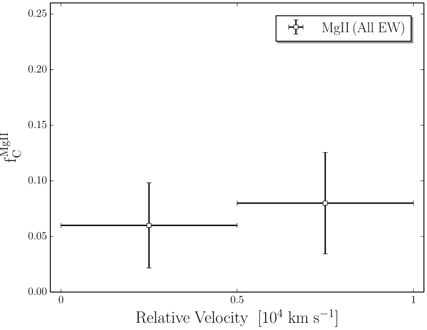
Figure 6: Covering fraction, f_C, for MgII $\lambda$ 2796 estimated from the fraction of quasars exhibiting at least one absorber in bins of velocity offset from z_em. The rest frame equivalent width detection limit (in the near-IR) in our sample is 0.036 Å  (see P16).

The detection fraction derived in Farina et al., 2014 (or Johnson et al., 2015) cannot be compared directly with our result. Indeed, the velocity offset of each MgII absorber detected in our survey cannot be translated directly into a physical separation from the quasar, because the redshift also includes information on its peculiar velocity. If we did that, we would derive a proper distance of the order of $\sim$10 Mpc, implying a lack of correlation between the absorption system and the quasar host galaxy. Probably, all the gas explored in those works is contained in our first bin, within 5000 km s^-1 of z_em. What is relevant is that we observe a dramatically different MgII covering fraction at any velocity separation that is reasonable to associate with gas within the host galaxy.

4.4 Importance of barycentre determination

In the previous sections, we have considered the position of the deepest component of each CIV system as the zero velocity point around which we select the regions to produce the stacked spectrum (as described in Section 3). Such barycentre selection is justified by the fact that low-ionization ions in our sample generally appear to be well-aligned with the deepest component of CIV systems that exhibit a complex velocity-component structure. Now, we explore how the stacking is affected by this choice (see also Ellison et al., 2000).

The deepest component of the CIV systems in our sample not always coincide with the centre of their velocity profiles. The most affected systems are those for which it is not possible to discern the individual narrow components within the adopted clustering velocity (see Section 2). They are usually the strongest systems in a given velocity bin and dominate the final composite spectrum. As a consequence, the stacked absorption profiles appear slightly asymmetric (see Fig. 4). In contrast, this trend does not affect the weak systems, which we are able to consider separately from each other.

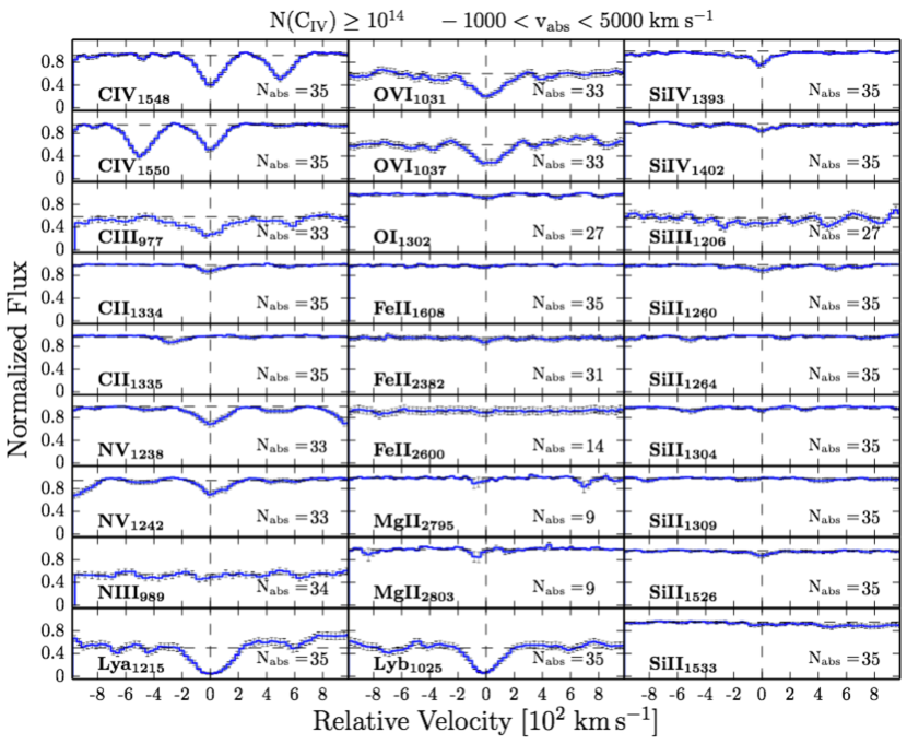
Figure 12: Composite spectra for the ions studied in this work, based on the CIV systems with N(CIV)$\geq$ 10¹⁴ cm^-2 and -1000 <v_abs< 5000 km s^-1. The barycentre position of each CIV system has been computed weighting the wavelengths with the optical depth of the line profile. Every panel reports the number of absorbers considered to build the stacked spectrum. The error bars are 1$\sigma$ and are estimated by bootstrapping the data using 1000 realizations.

We now calculate the barycentre position of each CIV system, weighting the wavelengths with the optical depth of the line profile. Fig. 12 in the Appendix shows the results. This technique produces more symmetric absorption troughs for the intermediate- and high-ionization ions. However, their profiles are broader and less representative of the width of direct individual detections. In addition, this method spreads out the signal of the low-ionization ions, making their signatures less evident and in some cases off-centered. This latter effect happens because most of the low-ionization ions are associated with DLA systems, and their absorption profile is often asymmetric. In conclusion, selecting the barycentre of the regions to be stacked according to the minimum of each CIV system, we produce much more coherent absorption signatures.

We also note that, while the NV stacked spectrum matches the kinematic profile of the corresponding CIV, the OVI absorption trough appears more irregular and broad (see Fig. 4). NV absorptions arise predominately at the same velocity as CIV, while OVI is often significantly shifted to positive velocities, at both high and low redshift (e.g. Fechner & Richter, 2009; Lopez et al., 2007; Carswell et al., 2002; Tripp et al., 2008 ). The usual interpretation of this often observed velocity shift between OVI and CIV (e.g. Reimers et al., 2001; Carswell et al., 2002; Simcoe et al., 2002) is that the lines do not arise from the same volume. However, the origin of the shift remains uncertain.

In summary, we find that the NV features in our sample are well-aligned with CIV, implying that both species arise from the same gas phase, whereas, velocity offsets between CIV and OVI centroids may contribute to producing a broader stacked profile compared to other species. We will discuss the possible origin of NV and OVI more extensively in Section 5.1.

5 DISCUSSION

In this article, we stack 100 quasar spectra in the rest-frame of CIV absorbers detected in the dataset of XQ-100 Legacy Survey, to examine the typical strength of NV and other lines in the vicinity of quasars compared with intervening gas. The combination of moderate resolution, high S/N and wide wavelength coverage of our survey have allowed us to build composite spectra at redshifts 2.55-4.73 and at the same time explore a wide range of strong and weak NALs.

From now on, we refer to the top panels of Fig. 5 (panels a and e) to describe the associated region for strong and weak systems, respectively. On the other hand, the bottom panels (panels d and h), characterize intervening gas. Fig. 5(d) and (h) correspond to a velocity offset from z_em (10,000 < v_abs < 35,000 km s^-1) that includes both the smaller bins explored in the two upper panels and is large enough to allow the investigated ions to produce measurable absorptions. Besides this, we are confident that in Fig. 5(d) and (h) only intervening systems are selected, because this velocity bin does not encompass the excess of NALs within 10,000 km s^-1 of z_em found in P16 (see Fig. 9 for more details). DLAs have been excluded from the stacking, since they represent a special class of systems.

AALs are characterized by higher ionization states than intervening absorbers. Indeed, we can see in Fig. 5 that NV exhibits a strong absorption signal only within 5000 km s^-1 of z_em. This absorption trough is much stronger if CIV systems with N(CIV) > 10¹⁴ cm^-2 are used to build the composite spectrum. We draw attention to the fact that OVI is detected in the proximity of the quasar, as well as in the intervening gas. This is not surprising, since OVI absorption is observed in a wide range of astrophysical environments (see Fox, 2011 for a review). However, the OVI/CIV ratio is higher in AALs. Fig. 5 also shows that SiIV is detected both in the proximity of the quasar and in intervening gas. Nevertheless, it is much weaker close to the quasar, where the gas is more easily ionized, and it is thus reasonable to expect that a smaller fraction of silicon is in the form of SiIV. We note that SiIII signal increases moving farther from the quasar and that the SiIV/SiIII and SiIV/CIV ratios suggest lower ionization in intervening systems with respect to associated ones. This is true for the composite spectra obtained selecting both weak and strong CIV systems. AALs are also characterized by the absence of the low-ionization ions. They are found, instead, at large velocity separation from the z_em, but only associated with the strongest CIV systems in the sample (i.e. N(CIV) > 10¹⁴ cm^-2). Indeed, low-ionisation metal transitions, such as MgII, CII and SiII, are mostly found at N(HI) $\geq$ 10¹⁶ cm^-2 (e.g. Farina et al., 2014).

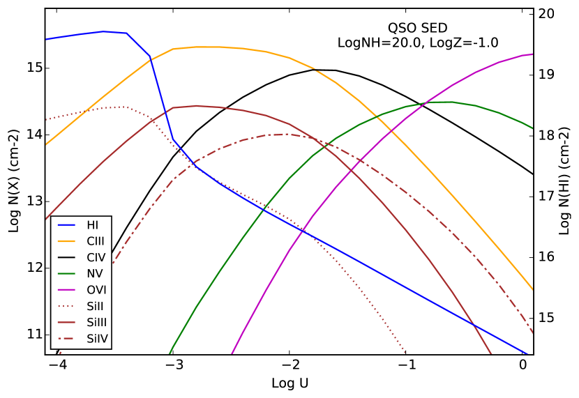
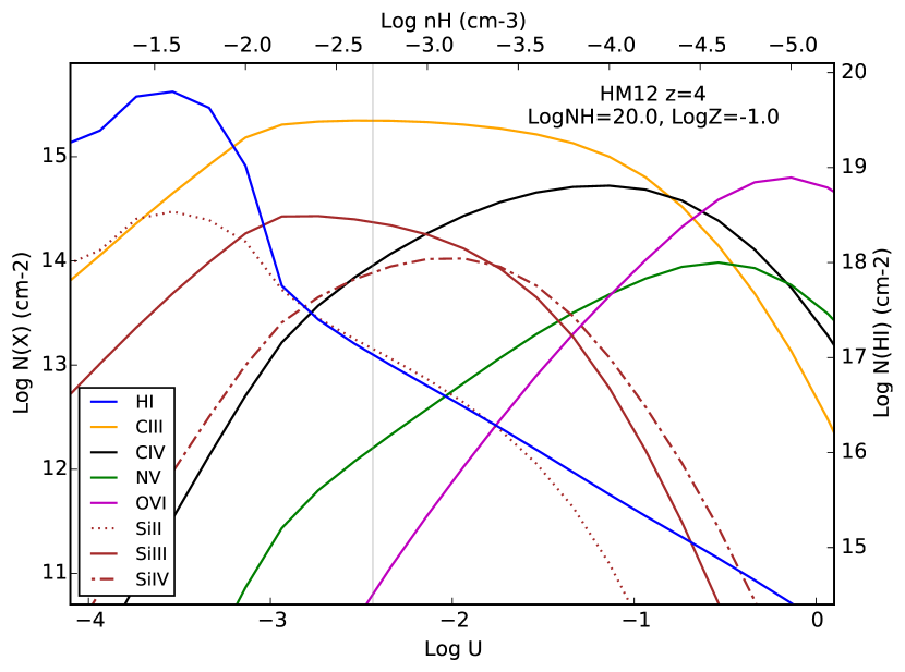
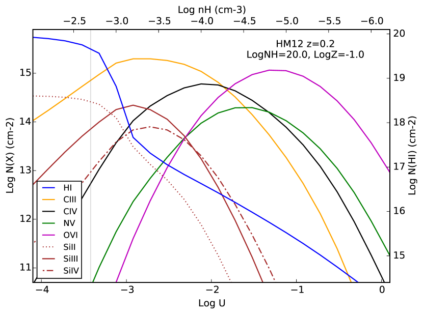
Figure 7: Cloudy-predicted column densities as a function of the ionization parameter U, for a cloud of total column density Log (N_H) = 20 cm^-2. The metallicity of the cloud is Log Z = $-$1.0 with solar relative abundances. The N(HI) is shown by the bold blue curve and axis labels on the right. Top panel: the gas is assumed to be photoionized by a quasar Spectral Energy Distribution. Middle and bottom panels: the gas is assumed to be photoionized by the UV background radiation (Haardt & Madau, 2012) at z = 4 (middle panel) and z = 0.2 (bottom panel).

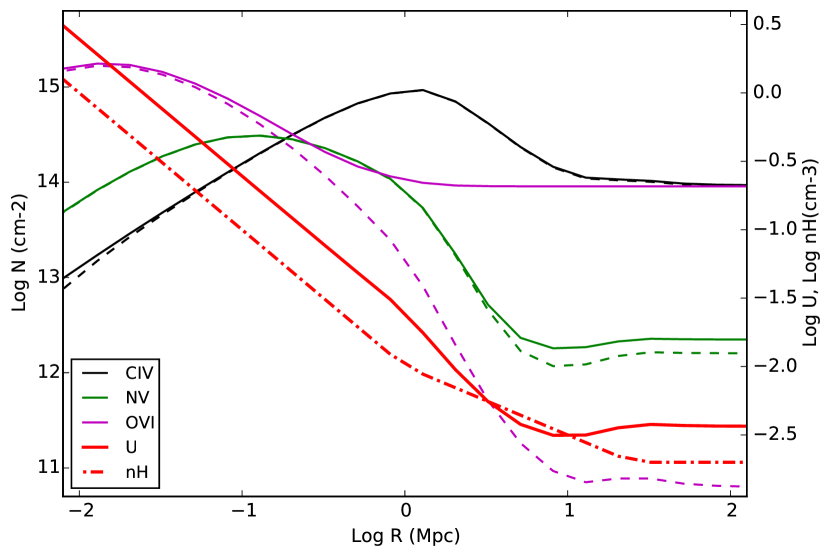
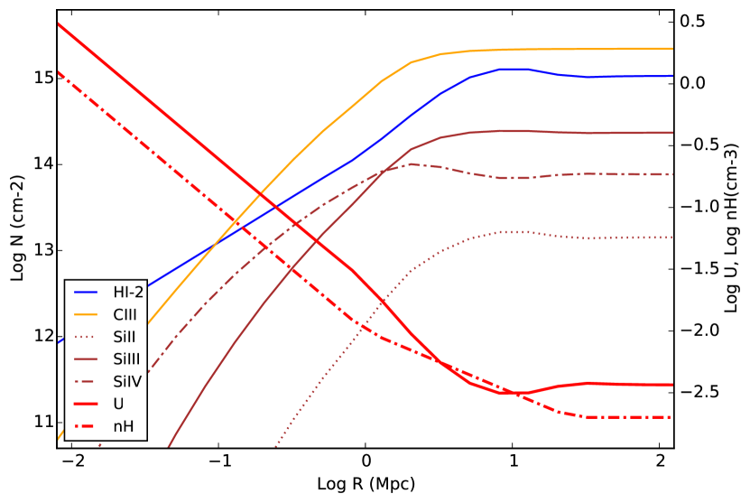
Figure 8: Cloudy-predicted column densities as a function of the distance, R, from a quasar at z = 4.The metallicity of the cloud is Log Z = $-$1.0 with solar relative abundances and the total column density is Log (N_H) = 20. The gas is modelled as a uniform slab in thermal and ionization equilibrium and is assumed to be photoionized by the radiation field of a quasar with bolometric luminosity L = 10⁴⁷ erg s^-1 and the UV background radiation (Haardt & Madau, 2012). We also add a thermal gas component with Log T = 5.5. The solid curves show the sum of the two contributions, while the dashed ones show just the photoionized component. The ions in the right panel are not affected by the thermal component. The HI column density, labeled “H1-2”, is plotted as Log N(HI) $-$ 2.0 to fit on the plot. The densities of the cloud and the U parameters at each R are shown by the dot-dashed and bold red curves, respectively, and axis labels on the right. Left: CIV, NV and OVI column densities. Right: low-ions column densities.

Fig. 5 clearly shows that the gas in the proximity of the quasar exhibits a considerably different ionization state with respect to the intervening gas. In order to illustrate how the absorption-line strengths of the explored ions vary as a function of different physical conditions, we use the Cloudy software package (v17.00; Ferland et al., 2017) to run ionization models.

A photoionized plasma is characterized by the ionization parameter, U = Q_H/4$\pi$R²n_Hc, where Q_H is the source emission rate of hydrogen ionizing photons, R is the distance from the central source, n_H is the hydrogen density and c is the speed of light. Top panel of Fig. 7 exhibits how the column densities of several ions within a cloud of total column density Log N(H) = 20 cm^-2, vary as a function of U. In this model, the gas is assumed to be photoionized only by the radiation field of the quasar. The adopted bolometric luminosity of the quasar is L = 10⁴⁷ erg s^-1, representative of the XQ-100 sample (see P16). We consider a metallicity Log Z = $-$1.0, with solar relative abundances. We note that, close to the quasar (high values of U), the intense and hard radiation field eliminates the low ions and allows nitrogen and oxygen to be highly ionized. Moving farther from the quasar, the decrease of U produces the drop of the NV and OVI absorption signal, and the appearance of the low-ions.

Fig. 8 illustrates this trend even better, showing how the column densities of the same ions vary as a function of the distance, R, from a quasar at z = 4 (properties of the cloud as in Fig. 7). The gas is assumed to be photoionized by the radiation field of the quasar and the UV background (Haardt & Madau, 2012). We also add a thermal gas component with Log T = 5.5 to mimic the effect of collisionally ionized gas. The dashed curves show the photoionized component, while the solid ones represent the sum of the two contributions.

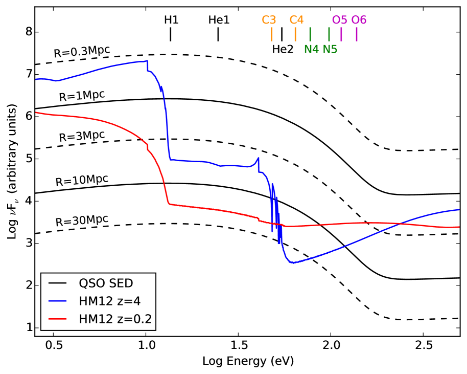
Figure 10: UV background (Haardt & Madau, 2012) spectral energy distribution (SED) at z = 4 and z = 0.2, and quasar SED scaled to different distances from the quasar. The tick marks along the top mark the ionization energies of some ions important for the discussion.

Let us focus on the photoionized component first. We can see in the left panel of Fig. 8 that NV and OVI (and slightly CIV) drop with distance from the quasar, because the gas is subjected to lower values of U (it corresponds to moving to the left in the top panel of Fig. 7). Those ions signal would continue to decrease, except that at large R they hit a floor determined by the UV background. Fig. 10 in the Appendix shows that the UV background at z = 4 starts to dominate the ionizing continuum (> 13.6 eV) at R $\gtrsim$ 3 Mpc, but its spectral energy distribution (SED) is strongly shaped by deep edges due to HI and HeII ionization. In particular, the CIII edge is at lower energies than the HeII one, so the UV background radiation at z = 4 can produce CIV, but it cannot produce much OVI and even less NV. The right panel of Fig. 8 shows how, moving away from the quasar, the decreases of U allows low-ions absorption signal to rise.

The trends illustrated in Fig. 8 give a natural explanation for the increase in SiIV/CIV and SiIII/SiIV ratios we see in Fig. 5 moving towards gas at large separation from the quasar. The substantial difference in the NV/CIV ratio between AAL and intervening systems is also well described. However, if the drop of U were the only factor in play, we should detect a much weaker OVI signal far from the z_em in our composite spectra. Indeed, the NV ionization potential is in between those of CIV and OVI and we can see in Fig. 5 that NV signal drops moving away from the quasar, while the OVI/CIV ratio is not subject to a change consistent with that of NV. This trend can have multiple interpretations.

One possibility is that OVI traces another phase of the absorbing gas, independently from the environment, and it has a different mechanism of production with respect to NV, so the change of the ionization radiation at large distance from the quasar affects only the NV signal. This is unlikely, since OVI is often found to be photoionized (e.g. Bergeron et al., 2002; Reimers et al., 2006; Fechner & Richter, 2009). It is also possible that OVI is photoionized in the proximity of the quasar and has a different channel of production in other environments.

Fig. 8 clearly illustrates that a thermal gas component with Log T = 5.5 increases N(OVI) significantly at large R (magenta curves), but it contributes little to N(NV) (green) and negligibly to N(CIV) (black). This model suggests that, moving farther from the quasar, the change in the U parameter causes the drop in both NV and OVI. The fact that we see an OVI signal in our composite spectra even at large velocity offsets from z_em can be explained by an additional thermal gas component.

Right panel of Fig. 5 shows that the lower N(CIV) systems have much higher CIII/CIV than the high N(CIV). Therefore, selecting weak CIV absorbers we do not simply find lower total column densities. We also find systems with lower ionization. However, this trend cannot be explained only by changing U, because the strong CIII and larger CIII/CIV ratios are not (clearly) accompanied by stronger absorption in other lower ions. All of these absorbers can have a range of n_H, which means a range in U values. So, from a distribution of absorbers, systems with weak CIV NALs and small CIV/CIII ratios might have relatively less of the low n_H, high U gas (not simply lower U overall).

5.1 NV and OVI as diagnostics of ionization mechanisms

Conclusions regarding the origin and fate of CGM are linked to the assumptions one makes about the physical processes that determine its ionization state. Successful models of the CGM must account for the full suite of observations available and combine together the two dominant gas phases, typically described as a cool $\sim$ 10⁴ K and a warm $\sim$ 3 $\times$ 10⁵ K phase. In this context, the presence or absence of NV and OVI in quasar absorption systems may provide crucial information for understanding the physical conditions of the absorbing gas. NV and OVI require 77.5 (97.9) and 113.9 (138.1) eV to be created via photoionization (to be destroyed), respectively, and their abundance peaks at 2 $\times$ 10⁵ and 3 $\times$ 10⁵ K for collisionally ionized gas (Gnat & Sternberg, 2007).

Lu & Savage (1993) performed a search for NV and OVI absorption based on a composite spectrum method. To this aim they exploited a total of 73 intervening CIV systems (with mean redshift $\langle$z$\rangle$ = 2.76) identified in 36 spectra from the survey by Sargent et al. (1989). The results of this study may apply to relatively strong systems, since only CIV absorbers with rest-frame equivalent width $\geq$ 0.3 Å  can be detected in those spectra. This work provided the first firm evidence for the presence of the OVI absorption in intervening quasar metal line systems, while NV doublet was not detected. This agrees with what we find in our composite spectrum obtained selecting only strong CIV absorbers. They estimated the ratio N(OVI)/N(NV) to be $\geq$ 4.4, which, for collisionally ionized gas in thermal equilibrium with a solar ratio of oxygen to nitrogen, implies a gas temperature T $\geq$ 2.5 $\times$ 10⁵ K.

More recently, many detailed studies have been carried out on an absorber-by-absorber basis in quasar spectra that trace low-density foreground gas in the IGM and galaxy halos. These studies have shown that the ionization mechanisms of high-ionization species like OVI and NV are complex and vary over a wide range of environments. Line diagnostics from low, intermediate, and high ions sometimes support a similar, photoionized origin for OVI, NV, and low-ionization state gas (e.g. Tripp et al., 2008; Muzahid et al., 2015) and sometimes require OVI to be ionized by collisions of electrons with ions in a $\sim$ 3 $\times$ 10⁵ K plasma (e.g. Tumlinson et al., 2005; Fox et al., 2009; Wakker et al., 2012; Meiring et al., 2013).

Recently, the work by Werk et al. (2016) reported on quasars probing sight lines near 24 star-forming galaxies with L $\approx$ L^∗ at z = 0.2 from the COS-Halos survey (Werk et al., 2013; Tumlinson et al., 2013), which exhibit positive detections of OVI in their inner CGM. Of the galaxies analysed, only three have positive detections of NV. They also argue about the possibility that NV does not trace the same gas phase as OVI, since they show different velocity profiles. However, a NV upper limit can impose meaningful constraints in both photoionized and collisionally ionized gas models. For example, the upper limits on Log N(NV)/N(OVI) $\sim$ $-$1 strongly rule out most photoionization models, both in and out of equilibrium. Bordoloi et al. (2017) claim that most of the observed COS-Halos OVI absorption-line systems can be explained as collisionally ionized gas radiatively cooling behind a shock or other type of radiatively cooling flow. Their model predicts the typical NV column densities to be an order of magnitude smaller than the OVI ones at similar cooling velocities. Therefore, most of the COS-Halos NV systems associated with OVI absorption would reside below the detection threshold, consistent with NV non-detection for the majority of the COS-Halos OVI. In the context of a multiphase CGM, however, this scenario does not take into account the constraints on the NV signal coming from photoionization models based on the low and intermediate ions.

Fig. 7 shows the Cloudy-predicted column densities of several ions as a function of the ionization parameter U, for a cloud of total column density Log (N_H) = 20 cm^-2, at z = 4 (middle panel) and z = 0.2 (bottom panel). We model a cloud with the same parameters as in Fig. 8, to investigate how the picture described at large separation from the quasar changes with redshift. The vertical grey line in the middle panel marks U and n_H reached at large distance in Fig. 8. We note that, considering the same U parameter, the Haardt & Madau (2012) spectrum produces more NV and OVI at low z. Fig. 10 in the Appendix shows that the UV background flux at energies from $\sim$13.6 eV to $\sim$45 eV is weaker at z = 0.2 by 0.98 dex compared with z = 4. However, for any given density, it produces $\sim$10 times lower U at z = 0.2 than at z = 4, but more NV and OVI, due to the harder continuum shape around the energies that create those ions. Single-phase photoionization models fail in explaining the range of N(NV)/N(OVI) reported by studies at low z (e.g. COS-Halos survey). As discussed in Werk et al. (2016), the observed Log N(NV)/N(OVI) $\sim$ $-$1 would require very low gas density for the CGM with U $\geq$ $-$1 (see the bottom panel of Fig. 7). However, depending on the physical condition of the cloud, the NV signal produced by photoionization can be an important contribution to the total strength of the absorbing line. Therefore, before using the NV non-detection to derive a limit on the gas temperature, one can exploit the constraints from low and intermediate ions to predict the NV absorption produced by the UV background radiation.

The details of the mechanisms that ionize the absorbing gas can rapidly get complex if non-equilibrium processes are occurring and/or if there is a combination of photoionization and collisional ionization (Savage et al., 2014, for a recent review). Among the models proposed to reproduce the intermediate- and high-ion states (e.g. CIV, NV, OVI) there are (1) time-variable radiation fields from AGN coupled with non-equilibrium ionization effects (Segers et al., 2017; Oppenheimer et al., 2017), (2) radiative cooling flows (Bordoloi et al., 2017; McQuinn & Werk, 2018), (3) formation in fast shocks (Gnat & Sternberg, 2009) or (4) formation within thermally conductive interfaces (Gnat et al., 2010; Armillotta et al., 2017).

We have shown that it is possible that NV is photoionized in environments where OVI is mostly collisionally ionized, but being weak it is hard to detect. We have also demonstrated that the observed differences in the NV/CIV ratio between AALs and intervening systems can be explained naturally by ionization effects. However, another factor that can contribute in making the intervening NV signal weaker than already expected is that these absorbers can trace gas in regions with lower metallicity or sub-solar N/$\alpha$ relative abundance. NV absorptions are largely identified in proximity to bright quasars along the line of sight (e.g. Misawa et al., 2007; Nestor et al., 2008; Ganguly et al., 2013, P16, Chen & Pan, 2017). Quasars are generally metal-rich and about solar [N/H] has been measured in associated systems (Petitjean et al., 1994; Dietrich et al., 2003; D’Odorico et al., 2004; Ganguly et al., 2006; Schaye et al., 2007), making NV easily detectable in proximate absorbers. Nitrogen is rarely detected in optically thin (i.e. N(HI) $\lesssim$ 10¹⁷ cm^-2) intergalactic absorption systems. In the IGM, the metallicity and therefore the nitrogen content is lower, thus NV features are expected to be weak (Fechner & Richter, 2009).

Fechner & Richter (2009) find that the [N/$\alpha$] abundance in intervening systems is clearly sub-solar, with a median [N/$\alpha$] = $-$0.58 and values down to $\sim$ $-$1.8. Observations have shown that the N/O ratio can diminish moving outwards of disc galaxies as a function of the galactocentric distance and stellar mass (e.g. Belfiore et al., 2017). This result is supported by chemical evolution models included within cosmological hydrodynamical simulations (Vincenzo & Kobayashi, 2018a, b). “Down the barrel” observations give us access to gas originated at small distances from the centre of the quasar host galaxy (e.g. Wu et al., 2010). In contrast, the absorption systems identified in works based on projected pairs usually have impact parameters from tens to hundreds of kpc from the z_em of the background target, so they trace gas in the outskirts of galaxies possibly characterized by a lower N/O ratio.

6 CONCLUSIONS

In this work, we present new measurements of metal NALs made using composite quasar spectra. Our sample includes 100 individual lines of sight from the XQ-100 Legacy survey, at emission redshift z_em = 3.5-4.72. To build the stacking spectra, we start from a large number ($\sim$ 1000) of CIV absorption systems identified in P16, covering the redshift range 2.55 < z_abs < 4.73. The main goal of our analysis is to investigate the NV absorption signal at large velocity separations from z_em. This study complement our previous work on NV and test the robustness of the use of NV as a criterion to select intrinsic NALs. We also characterize the ionization state of the gas, both near and at great distance from the quasar. Our primary results are as follows.

(1) We show the absence of a statistically significant intervening NV absorption signal along the line of sight of background quasars. Indeed, the NV exhibits a strong absorption trough only within 5000 km s^-1 of z_em. This feature is much stronger ($\sim$ 15$\sigma$ confidence level) if CIV systems with N(CIV) > 10¹⁴ cm^-2 are considered to build the composite spectrum. This result supports our previous claim (see P16) that NV is an excellent statistical tool for identifying intrinsic systems.

(2) We use photoionization models to show that, in a scenario where associated systems are photoionized by a quasar, the ionization parameter is expected to drop dramatically with distance from the continuum source. This is the main reason for intervening NV systems being weaker than associated ones. Another possible contribution to this trend is a lower metallicity or N/O abundance.

( 3) The gas close to the continuum source (v_abs < 5000 km s^-1) exhibits a different ionization state with respect to the intervening one. Moving farther from the quasar, we can appreciate the appearance of the low-ions associated with the strongest systems in the sample (N(CIV) > 10¹⁴ cm^-2) and the drop in the NV absorption signal. In contrast, the OVI NAL is detected even at large velocity shifts from z_em. We also note that OVI and CIV do not exhibit a change in their absorption signal in line with the decrease of the NV signal. We run photoionization models that describe these trends well (see Fig.8). We use these models to illustrate that a drop in the U parameter cannot be the only element to explain the data and that an additional thermal component (T $\sim$ 3 $\times$ 10⁵ K) can produce the OVI absorption we detect at large distance from the quasar. We show how it is possible that NV is photoionized in environments where OVI is mostly collisionally ionized, but, being weak, this can be challenging to detect.

(4) We verify the deficiency of cool gas, as traced by low ions and in particular by MgII, in the proximity of the quasar. This finding is in agreement with the dearth of CII NALs (as shown in P16) and confirms that the gas in the proximity of the quasar along the line of sight has a different ionization state with respect to the gas in the transverse direction (e.g. Prochaska et al., 2014; Farina et al., 2014).

Appendix A

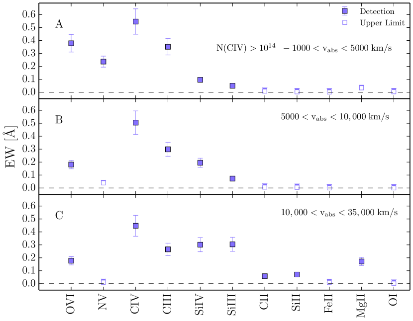
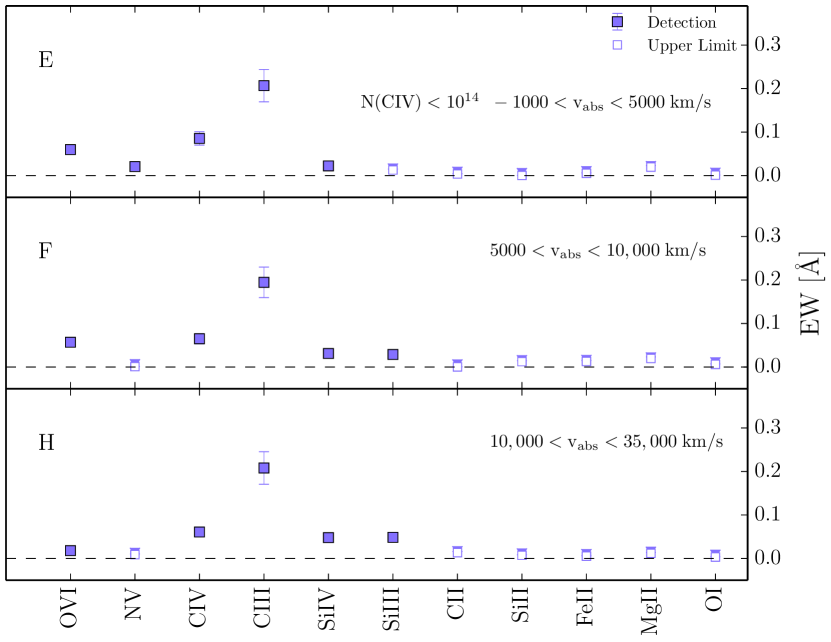
Figure 9: Left: The equivalent widths of metal species measured in order of decreasing ionization potential for composite spectra based on the CIV systems with N(CIV)$\geq$ 10¹⁴ cm^-2. Each panel displays the velocity offset from z_em. CIV DLAs have been excluded form the stacking. Right: same as for the left panels, but in this case N(CIV)< 10¹⁴ cm^-2 is considered as threshold for the stacking. The EW refers only to the strongest member of the doublets. Error bars are 1$\sigma$ and are estimated by bootstrapping the data using 1000 realizations.

The left panels of Fig. 9 show the rest-frame equivalent widths of metal species measured in the composite spectrum based on CIV systems with N(CIV) $\geq$ 10¹⁴ cm^-2 and 5000 < v_abs < 10,000 km s^-1 (panel b), compared to results for AAL and intervening systems (panels a and c), already presented in Fig. 5. The right panels are the same as the left panels, but in this case N(CIV) < 10¹⁴ cm^-2 is considered as threshold for the stacking. The 5000 < v_abs < 10,000 km s^-1 is a particular velocity bin in our study. In P16 we find that the CIV sample exhibits a statistically significant excess ($\sim$ 8$\sigma$) within 10,000 km s^-1 of z_em with respect to the random occurrence of NALs, which is especially evident for lines with EW < 0.2 Å. These latter lines more or less correspond to the weak systems in the current study. The excess extends to larger velocities than the classical associated region, is not an effect of NAL redshift evolution and does not show a significant dependence from the quasar bolometric luminosity.

We note that the systems in the 5000 < v_abs < 10,000 km s^-1 bin exhibit some of the properties of the associated systems and at the same time they show some characteristics of the intervening ones. Let us focus on the strong systems first. Fig. 9(b) shows that the CIV/SiIV and CIV/SiIII ratios are close to those of the AALs (Fig. 9a), but OVI/CIV and NV/CIV ratios are in line with those of the intervening gas (Fig. 9c). In addition, we only measure upper limits for the low ions, in agreement with gas in the proximity of the quasar. If we consider weak systems, Fig. 9(f) shows a smaller CIV/SiIII ratio like intervening gas, but a larger value of the OVI absorption like the AALs.

Fig. 9(b) and (f) seem to represent a "transition" region between associated and intervening systems. The EWs shown in those bins are produced by averaging together absorbers physically connected with the quasar host galaxy and its halo and spurious intervening systems. This is the main reason why we excluded this bin from our stacking analysis.

References

- Aguirre et al. (2004) Aguirre A., Schaye J., Kim T.-S., Theuns T., Rauch M., Sargent W. L. W., 2004, ApJ, 602, 38
- Aguirre et al. (2008) Aguirre A., Dow-Hygelund C., Schaye J., Theuns T., 2008, ApJ, 689, 851
- Anderson et al. (1987) Anderson S. F., Weymann R. J., Foltz C. B., Chaffee Jr. F. H., 1987, AJ, 94, 278
- Antonucci (1993) Antonucci R., 1993, ARA&A, 31, 473
- Armillotta et al. (2017) Armillotta L., Fraternali F., Werk J. K., Prochaska J. X., Marinacci F., 2017, MNRAS, 470, 114
- Becker et al. (2013) Becker G. D., Hewett P. C., Worseck G., Prochaska J. X., 2013, MNRAS, 430, 2067
- Belfiore et al. (2017) Belfiore F., et al., 2017, MNRAS, 469, 151
- Berg et al. (2016) Berg T. A. M., et al., 2016, MNRAS, 463, 3021
- Berg et al. (2017) Berg T. A. M., et al., 2017, MNRAS, 464, L56
- Berg et al. (2018) Berg T. A. M., Ellison S. L., Tumlinson J., Oppenheimer B. D., Horton R., Bordoloi R., Schaye J., 2018, MNRAS,
- Bergeron et al. (2002) Bergeron J., Aracil B., Petitjean P., Pichon C., 2002, A&A, 396, L11
- Bordoloi et al. (2017) Bordoloi R., Wagner A. Y., Heckman T. M., Norman C. A., 2017, ApJ, 848, 122
- Bouché et al. (2012) Bouché N., Hohensee W., Vargas R., Kacprzak G. G., Martin C. L., Cooke J., Churchill C. W., 2012, MNRAS, 426, 801
- Bowen et al. (2006) Bowen D. V., et al., 2006, ApJ, 645, L105
- Bowen et al. (2008) Bowen D. V., et al., 2008, ApJS, 176, 59
- Burchett et al. (2015) Burchett J. N., et al., 2015, ApJ, 815, 91
- Carswell et al. (2002) Carswell B., Schaye J., Kim T.-S., 2002, ApJ, 578, 43
- Charlton et al. (2000) Charlton J. C., Churchill C. W., Rigby J. R., 2000, ApJ, 544, 702
- Chelouche et al. (2008) Chelouche D., Ménard B., Bowen D. V., Gnat O., 2008, ApJ, 683, 55
- Chen & Pan (2017) Chen Z.-F., Pan D.-S., 2017, ApJ, 848, 79
- Chen et al. (2018) Chen Z.-F., Huang W.-R., Pang T.-T., Huang H.-Y., Pan D.-S., Yao M., Nong W.-J., Lu M.-M., 2018, ApJS, 235, 11
- Cowie et al. (1995) Cowie L. L., Songaila A., Kim T.-S., Hu E. M., 1995, AJ, 109, 1522
- Crenshaw et al. (1999) Crenshaw D. M., Kraemer S. B., Boggess A., Maran S. P., Mushotzky R. F., Wu C.-C., 1999, ApJ, 516, 750
- D’Odorico et al. (2004) D’Odorico V., Cristiani S., Romano D., Granato G. L., Danese L., 2004, MNRAS, 351, 976
- D’Odorico et al. (2016) D’Odorico V., et al., 2016, MNRAS, 463, 2690
- Danforth & Shull (2008) Danforth C. W., Shull J. M., 2008, ApJ, 679, 194
- Davé et al. (1998) Davé R., Hellsten U., Hernquist L., Katz N., Weinberg D. H., 1998, ApJ, 509, 661
- Di Matteo et al. (2005) Di Matteo T., Springel V., Hernquist L., 2005, Nature, 433, 604
- Dietrich et al. (2003) Dietrich M., Appenzeller I., Hamann F., Heidt J., Jäger K., Vestergaard M., Wagner S. J., 2003, A&A, 398, 891
- Ellison et al. (2000) Ellison S. L., Songaila A., Schaye J., Pettini M., 2000, AJ, 120, 1175
- Elvis (2000) Elvis M., 2000, ApJ, 545, 63
- Farina et al. (2013) Farina E. P., Falomo R., Decarli R., Treves A., Kotilainen J. K., 2013, MNRAS, 429, 1267
- Farina et al. (2014) Farina E. P., Falomo R., Scarpa R., Decarli R., Treves A., Kotilainen J. K., 2014, MNRAS, 441, 886
- Faucher-Giguère & Kereš (2011) Faucher-Giguère C.-A., Kereš D., 2011, MNRAS, 412, L118
- Faucher-Giguère et al. (2008) Faucher-Giguère C.-A., Lidz A., Hernquist L., Zaldarriaga M., 2008, ApJ, 688, 85
- Fechner & Richter (2009) Fechner C., Richter P., 2009, A&A, 496, 31
- Ferland et al. (2017) Ferland G. J., et al., 2017, Rev. Mex. Astron. Astrofis., 53, 385
- Foltz et al. (1986) Foltz C. B., Weymann R. J., Peterson B. M., Sun L., Malkan M. A., Chaffee Jr. F. H., 1986, ApJ, 307, 504
- Fontana & Ballester (1995) Fontana A., Ballester P., 1995, The Messenger, 80, 37
- Fox (2011) Fox A. J., 2011, ApJ, 730, 58
- Fox et al. (2005) Fox A. J., Savage B. D., Wakker B. P., 2005, AJ, 130, 2418
- Fox et al. (2007) Fox A. J., Petitjean P., Ledoux C., Srianand R., 2007, A&A, 465, 171
- Fox et al. (2008) Fox A. J., Ledoux C., Vreeswijk P. M., Smette A., Jaunsen A. O., 2008, A&A, 491, 189
- Fox et al. (2009) Fox A. J., Prochaska J. X., Ledoux C., Petitjean P., Wolfe A. M., Srianand R., 2009, A&A, 503, 731
- Fumagalli et al. (2011) Fumagalli M., Prochaska J. X., Kasen D., Dekel A., Ceverino D., Primack J. R., 2011, MNRAS, 418, 1796
- Fumagalli et al. (2014) Fumagalli M., Hennawi J. F., Prochaska J. X., Kasen D., Dekel A., Ceverino D., Primack J., 2014, ApJ, 780, 74
- Ganguly & Brotherton (2008) Ganguly R., Brotherton M. S., 2008, ApJ, 672, 102
- Ganguly et al. (2001) Ganguly R., Bond N. A., Charlton J. C., Eracleous M., Brandt W. N., Churchill C. W., 2001, ApJ, 549, 133
- Ganguly et al. (2006) Ganguly R., Sembach K. R., Tripp T. M., Savage B. D., Wakker B. P., 2006, ApJ, 645, 868
- Ganguly et al. (2013) Ganguly R., et al., 2013, MNRAS, 435, 1233
- Gnat & Sternberg (2007) Gnat O., Sternberg A., 2007, ApJS, 168, 213
- Gnat & Sternberg (2009) Gnat O., Sternberg A., 2009, ApJ, 693, 1514
- Gnat et al. (2010) Gnat O., Sternberg A., McKee C. F., 2010, ApJ, 718, 1315
- Granato et al. (2004) Granato G. L., De Zotti G., Silva L., Bressan A., Danese L., 2004, ApJ, 600, 580
- Gunn & Peterson (1965) Gunn J. E., Peterson B. A., 1965, ApJ, 142, 1633
- Haardt & Madau (2012) Haardt F., Madau P., 2012, ApJ, 746, 125
- Hamann & Ferland (1999) Hamann F., Ferland G., 1999, ARA&A, 37, 487
- Hamann et al. (1997) Hamann F., Beaver E. A., Cohen R. D., Junkkarinen V., Lyons R. W., Burbidge E. M., 1997, ApJ, 488, 155
- Hennawi & Prochaska (2007) Hennawi J. F., Prochaska J. X., 2007, ApJ, 655, 735
- Hennawi & Prochaska (2013) Hennawi J. F., Prochaska J. X., 2013, ApJ, 766, 58
- Hennawi et al. (2006) Hennawi J. F., et al., 2006, ApJ, 651, 61
- Hoopes et al. (2002) Hoopes C. G., Sembach K. R., Howk J. C., Savage B. D., Fullerton A. W., 2002, ApJ, 569, 233
- Hopkins & Elvis (2010) Hopkins P. F., Elvis M., 2010, MNRAS, 401, 7
- Hopkins et al. (2016) Hopkins P. F., Torrey P., Faucher-Giguère C.-A., Quataert E., Murray N., 2016, MNRAS, 458, 816
- Indebetouw & Shull (2004) Indebetouw R., Shull J. M., 2004, ApJ, 605, 205
- Jenkins (1996) Jenkins E. B., 1996, ApJ, 471, 292
- Jenkins et al. (2005) Jenkins E. B., Bowen D. V., Tripp T. M., Sembach K. R., 2005, ApJ, 623, 767
- Johnson et al. (2015) Johnson S. D., Chen H.-W., Mulchaey J. S., 2015, MNRAS, 452, 2553
- Kacprzak & Churchill (2011) Kacprzak G. G., Churchill C. W., 2011, ApJ, 743, L34
- Kim et al. (2016) Kim T.-S., Carswell R. F., Mongardi C., Partl A. M., Mücket J. P., Barai P., Cristiani S., 2016, MNRAS, 457, 2005
- King (2003) King A., 2003, ApJ, 596, L27
- Kirkman et al. (2005) Kirkman D., et al., 2005, MNRAS, 360, 1373
- Krogager et al. (2016) Krogager J.-K., Fynbo J. P. U., Noterdaeme P., Zafar T., Møller P., Ledoux C., Krühler T., Stockton A., 2016, MNRAS, 455, 2698
- Lau et al. (2016) Lau M. W., Prochaska J. X., Hennawi J. F., 2016, ApJS, 226, 25
- Lau et al. (2018) Lau M. W., Prochaska J. X., Hennawi J. F., 2018, The Astrophysical Journal, 857, 126
- Lehner & Howk (2011) Lehner N., Howk J. C., 2011, Science, 334, 955
- Lehner et al. (2009) Lehner N., Prochaska J. X., Kobulnicky H. A., Cooksey K. L., Howk J. C., Williger G. M., Cales S. L., 2009, ApJ, 694, 734
- Lehner et al. (2013) Lehner N., et al., 2013, ApJ, 770, 138
- Levshakov et al. (2003) Levshakov S. A., Agafonova I. I., D’Odorico S., Wolfe A. M., Dessauges-Zavadsky M., 2003, ApJ, 582, 596
- Lopez et al. (2007) Lopez S., Ellison S., D’Odorico S., Kim T.-S., 2007, A&A, 469, 61
- López et al. (2016) López S., et al., 2016, A&A, 594, A91
- Lu & Savage (1993) Lu L., Savage B. D., 1993, ApJ, 403, 127
- Lu et al. (1998) Lu L., Sargent W. L. W., Barlow T. A., Rauch M., 1998, ArXiv Astrophysics e-prints,
- McConnell & Ma (2013) McConnell N. J., Ma C.-P., 2013, ApJ, 764, 184
- McQuinn & Werk (2018) McQuinn M., Werk J. K., 2018, ApJ, 852, 33
- Meiring et al. (2013) Meiring J. D., Tripp T. M., Werk J. K., Howk J. C., Jenkins E. B., Prochaska J. X., Lehner N., Sembach K. R., 2013, ApJ, 767, 49
- Misawa et al. (2007) Misawa T., Charlton J. C., Eracleous M., Ganguly R., Tytler D., Kirkman D., Suzuki N., Lubin D., 2007, ApJS, 171, 1
- Morton (2003) Morton D. C., 2003, ApJS, 149, 205
- Murray et al. (2005) Murray N., Quataert E., Thompson T. A., 2005, ApJ, 618, 569
- Muzahid et al. (2015) Muzahid S., Kacprzak G. G., Churchill C. W., Charlton J. C., Nielsen N. M., Mathes N. L., Trujillo-Gomez S., 2015, ApJ, 811, 132
- Nestor et al. (2008) Nestor D., Hamann F., Rodriguez Hidalgo P., 2008, MNRAS, 386, 2055
- Netzer (2015) Netzer H., 2015, ARA&A, 53, 365
- Oppenheimer et al. (2017) Oppenheimer B. D., Schaye J., Crain R. A., Werk J. K., Richings A. J., 2017, preprint, (arXiv:1709.07577)
- Ostriker & Gnedin (1996) Ostriker J. P., Gnedin N. Y., 1996, ApJ, 472, L63
- Perrotta et al. (2016) Perrotta S., et al., 2016, MNRAS, 462, 3285
- Petitjean et al. (1994) Petitjean P., Rauch M., Carswell R. F., 1994, A&A, 291, 29
- Pieri et al. (2010) Pieri M. M., Frank S., Weinberg D. H., Mathur S., York D. G., 2010, ApJ, 724, L69
- Pieri et al. (2014) Pieri M. M., et al., 2014, MNRAS, 441, 1718
- Planck Collaboration et al. (2014) Planck Collaboration et al., 2014, A&A, 571, A16
- Prochaska & Hennawi (2009) Prochaska J. X., Hennawi J. F., 2009, ApJ, 690, 1558
- Prochaska & Wolfe (1997) Prochaska J. X., Wolfe A. M., 1997, ApJ, 487, 73
- Prochaska et al. (2006) Prochaska J. X., Chen H.-W., Bloom J. S., 2006, ApJ, 648, 95
- Prochaska et al. (2008) Prochaska J. X., Dessauges-Zavadsky M., Ramirez-Ruiz E., Chen H.-W., 2008, ApJ, 685, 344
- Prochaska et al. (2010) Prochaska J. X., O’Meara J. M., Worseck G., 2010, ApJ, 718, 392
- Prochaska et al. (2011) Prochaska J. X., Weiner B., Chen H.-W., Cooksey K. L., Mulchaey J. S., 2011, ApJS, 193, 28
- Prochaska et al. (2013) Prochaska J. X., et al., 2013, ApJ, 776, 136
- Prochaska et al. (2014) Prochaska J. X., Lau M. W., Hennawi J. F., 2014, ApJ, 796, 140
- Reimers et al. (2001) Reimers D., Baade R., Hagen H.-J., Lopez S., 2001, A&A, 374, 871
- Reimers et al. (2006) Reimers D., Agafonova I. I., Levshakov S. A., Hagen H.-J., Fechner C., Tytler D., Kirkman D., Lopez S., 2006, A&A, 449, 9
- Ribaudo et al. (2011) Ribaudo J., Lehner N., Howk J. C., 2011, ApJ, 736, 42
- Runnoe et al. (2012) Runnoe J. C., Brotherton M. S., Shang Z., 2012, MNRAS, 422, 478
- Sánchez-Ramírez et al. (2016) Sánchez-Ramírez R., et al., 2016, MNRAS, 456, 4488
- Sargent et al. (1989) Sargent W. L. W., Steidel C. C., Boksenberg A., 1989, ApJS, 69, 703
- Savage & Lehner (2006) Savage B. D., Lehner N., 2006, ApJS, 162, 134
- Savage & Sembach (1991) Savage B. D., Sembach K. R., 1991, ApJ, 379, 245
- Savage et al. (1997) Savage B. D., Sembach K. R., Lu L., 1997, AJ, 113, 2158
- Savage et al. (2003) Savage B. D., et al., 2003, ApJS, 146, 125
- Savage et al. (2005) Savage B. D., Lehner N., Wakker B. P., Sembach K. R., Tripp T. M., 2005, ApJ, 626, 776
- Savage et al. (2014) Savage B. D., Kim T.-S., Wakker B. P., Keeney B., Shull J. M., Stocke J. T., Green J. C., 2014, ApJS, 212, 8
- Scannapieco & Oh (2004) Scannapieco E., Oh S. P., 2004, ApJ, 608, 62
- Schaye et al. (2003) Schaye J., Aguirre A., Kim T.-S., Theuns T., Rauch M., Sargent W. L. W., 2003, ApJ, 596, 768
- Schaye et al. (2007) Schaye J., Carswell R. F., Kim T.-S., 2007, MNRAS, 379, 1169
- Segers et al. (2017) Segers M. C., Oppenheimer B. D., Schaye J., Richings A. J., 2017, MNRAS, 471, 1026
- Sembach & Savage (1992) Sembach K. R., Savage B. D., 1992, ApJS, 83, 147
- Sembach et al. (2003) Sembach K. R., et al., 2003, ApJS, 146, 165
- Shen & Ménard (2012) Shen Y., Ménard B., 2012, ApJ, 748, 131
- Simcoe et al. (2002) Simcoe R. A., Sargent W. L. W., Rauch M., 2002, ApJ, 578, 737
- Songaila (1998) Songaila A., 1998, AJ, 115, 2184
- Springel & Hernquist (2003) Springel V., Hernquist L., 2003, MNRAS, 339, 289
- Steidel (1990) Steidel C. C., 1990, ApJS, 74, 37
- Stocke et al. (2010) Stocke J. T., Keeney B. A., Danforth C. W., 2010, Publ. Astron. Soc. Australia, 27, 256
- Stocke et al. (2014) Stocke J. T., et al., 2014, ApJ, 791, 128
- Suzuki et al. (2005) Suzuki N., Tytler D., Kirkman D., O’Meara J. M., Lubin D., 2005, ApJ, 618, 592
- Thilker et al. (2004) Thilker D. A., Braun R., Walterbos R. A. M., Corbelli E., Lockman F. J., Murphy E., Maddalena R., 2004, ApJ, 601, L39
- Tripp et al. (2000) Tripp T. M., Savage B. D., Jenkins E. B., 2000, ApJ, 534, L1
- Tripp et al. (2008) Tripp T. M., Sembach K. R., Bowen D. V., Savage B. D., Jenkins E. B., Lehner N., Richter P., 2008, ApJS, 177, 39
- Tripp et al. (2011) Tripp T. M., et al., 2011, Science, 334, 952
- Tumlinson et al. (2005) Tumlinson J., Shull J. M., Giroux M. L., Stocke J. T., 2005, ApJ, 620, 95
- Tumlinson et al. (2011) Tumlinson J., et al., 2011, Science, 334, 948
- Tumlinson et al. (2013) Tumlinson J., et al., 2013, ApJ, 777, 59
- Turner et al. (2014) Turner M. L., Schaye J., Steidel C. C., Rudie G. C., Strom A. L., 2014, MNRAS, 445, 794
- Vernet et al. (2011) Vernet J., et al., 2011, A&A, 536, A105
- Vestergaard (2003) Vestergaard M., 2003, ApJ, 599, 116
- Vincenzo & Kobayashi (2018a) Vincenzo F., Kobayashi C., 2018a, preprint, (arXiv:1801.07911)
- Vincenzo & Kobayashi (2018b) Vincenzo F., Kobayashi C., 2018b, A&A, 610, L16
- Wakker et al. (2012) Wakker B. P., Savage B. D., Fox A. J., Benjamin R. A., Shapiro P. R., 2012, ApJ, 749, 157
- Weinberger et al. (2017) Weinberger R., et al., 2017, MNRAS, 465, 3291
- Werk et al. (2013) Werk J. K., Prochaska J. X., Thom C., Tumlinson J., Tripp T. M., O’Meara J. M., Peeples M. S., 2013, ApJS, 204, 17
- Werk et al. (2014) Werk J. K., et al., 2014, ApJ, 792, 8
- Werk et al. (2016) Werk J. K., et al., 2016, ApJ, 833, 54
- Wild et al. (2008) Wild V., et al., 2008, MNRAS, 388, 227
- Wu et al. (2010) Wu J., Charlton J. C., Misawa T., Eracleous M., Ganguly R., 2010, ApJ, 722, 997