Finite-Temperature Charge Dynamics and the Melting of the Mott Insulator

Abstract

The Mott insulator is the quintessential strongly correlated electronic state. We obtain complete insight into the physics of the two-dimensional Mott insulator by extending the slave-fermion (holon-doublon) description to finite temperatures. We first benchmark its predictions against state-of-the-art quantum Monte Carlo simulations, demonstrating quantitative agreement. Qualitatively, the short-ranged spin fluctuations both induce holon-doublon bound states and renormalize the charge sector to form the Hubbard bands. The Mott gap is understood as the charge gap renormalized downwards by these spin fluctuations. As temperature increases, the Mott gap closes before the charge gap, causing a pseudogap regime to appear naturally during the melting of the Mott insulator.

I Introduction

The Mott insulator Mott-1937 and its associated metal-insulator transition (MIT) Mott-1949 ; Mott-1956 ; Imada-1998 are phenomena generic to strongly correlated electron systems. The discovery Bednorz-1986 of high-$T_{c}$ superconductivity in a class of quasi-two-dimensional (quasi-2D) doped Mott insulators Lee-2006 triggered an enduring experimental and theoretical quest to understand the many anomalous properties of cuprates, including the strange metal, the pseudogap Damascelli-2003 ; Norman-2005 ; Sawatzky-2008 , and indeed the superconductivity itself, in a complete and correct description of the Mott insulator.

In Mott’s original proposal Mott-1990 , the insulating state arises due to the strong on-site Coulomb interaction, $U$, and has no explicit relation to symmetry-breaking (usually magnetic order). Hubbard Hubbard-1963 obtained the incoherent upper and lower Hubbard bands and considered the interaction-driven MIT, while Brinkman and Rice associated the MIT with a diverging quasiparticle mass Brinkman-1970 . These seminal results do not, however, include the spin fluctuations and their influence on the charge dynamics. In experiment, most Mott insulators possess antiferromagnetic (AFM) long-range order at low temperatures Imada-1998 . In 2D, where order is forbidden at $T>0$, the low-energy physics is dominated by short-ranged spin fluctuations Huscroft-2001 ; Moukouri-2001 ; Kyung-2006 ; Park-2008 ; Sordi-2010 ; Gunnarsson-2015 . On the scale of $U$, charge fluctuations create empty sites (holons) and doubly-occupied sites (doublons), whose tendency to form bound states has been proposed as the key to the high-energy physics of the Mott insulator Castellani-1979 ; Kaplan-1982 ; Capello-2005 ; Yokoyama-2006 ; Phillips-2010 ; Sen-2014 ; Peter-2015 ; Han-2016 . Clearly a full description requires a proper account of both charge and spin fluctuations Kotliar-1986 . While progress has been made in this direction through the development of many sophisticated numerical methods LeBlanc-2015 , a physical understanding remains far from complete.

Here we provide this insight by treating the half-filled Hubbard model within a slave-fermion formulation, in which the charge degrees of freedom are represented by fermionic holons and doublons, while the spin degrees of freedom are bosonic. To demonstrate that this framework provides quantitatively accurate resuls at the mean-field level for all temperatures, we perform detailed determinantal quantum Monte Carlo (QMC) simulations for benchmarking purposes. The key capability of our analytical approach is that it treats both the low- (spin) and high-energy (charge) degrees of freedom consistently, thereby capturing qualitative effects that arise due exclusively to their interplay, which to date have been accessible only by numerical methods.

By inspecting the physical content of the holon-doublon description, we are able to unveil the phenomenology of the Mott-insulating state. Our primary conclusions are as follows. Long-ranged AFM order is not required, because short-ranged spin fluctuations induce holon-doublon bound states. These fluctuations renormalize the charge sector to produce a Mott gap that is smaller than the charge gap. This reconstruction of the electronic states produces a quasiparticle, the “generalized spin polaron,” at the Hubbard-band edges, while most of the composite states lie higher in energy. The differing thermal evolution of the two gaps explains the origin of the pseudogap in the Mott insulator, which is a generic property at half-filling as well as at finite doping. The mixing of energy scales long observed to be at the heart of the complications endemic to a theoretical treatment of the Mott-insulating state is shown to be a “leverage” effect intrinsic to the convolution of charge and spin sectors that forms the reconstruction process.

The structure of this article is as follows. In Sec. II we introduce the slave-fermion description we use to analyze the Hubbard model at finite temperatures. In Sec. III we present details of our QMC techniques and apply these to benchmark our holon-doublon calculations. Having achieved a quantitative validation of its relevance, in Sec. IV we use the slave-fermion framework to deconstruct the single-particle excitations of the Mott insulator into their charge and spin components and to investigate their reconstruction over the full range of temperatures. In Sec. V we discuss the emergence of the pseudogap regime from the slave-fermion analysis and extract the intrinsic physics of the Mott insulator in terms of quasiparticle reconstruction and energy-scale leverage. Section VI contains a short summary and perspective.

II Hubbard model: Slave-fermion formalism when $T>0$

The Hamiltonian for the one-band Hubbard model is

$$H=-t\sum_{\langle i,j\rangle\sigma}c_{i\sigma}^{\dagger}c_{j\sigma}+U\sum_{i}(n_{i\uparrow}-{\textstyle\frac{1}{2}})(n_{i\downarrow}-{\textstyle\frac{1}{2}}),$$ (1)

where $c_{i\sigma}^{\dagger}$ creates an electron with spin $\sigma$ on site $i$ and $\langle i,j\rangle$ indicates only nearest-neighbor hopping, whose amplitude, $t=1$, sets the unit of energy. In the large-$U$ limit, the half-filled Hubbard model can be mapped to the AFM Heisenberg model Auerbach-1994 , $H_{S}=J\sum_{\langle i,j\rangle}\mathbf{S}_{i}\cdot\mathbf{S}_{j}$, and we assume that the spin dynamics are governed by this model also at finite $U$, taking $J=4t^{2}/U$.

The application of slave-particle decompositions to the Hubbard model [Eq. (1)] has a long history, which is reviewed briefly in Ref. Han-2016 . While in general the attribution of fermionic or bosonic statistics to the charge and spin components of the electron is arbitrary, for studies constrained to and about the mean-field level it was found shortly after the discovery of high-temperature superconductivity in cuprates Bednorz-1986 that the slave-fermion decomposition is more appropriate for the low-doped regime dominated by magnetic order (or correlations), while the superconducting and strange-metal regime is better described by the slave-boson decomposition Lee-2006 . For the present purposes, the magnetic fluctuations of the $S=1/2$ square-lattice antiferromagnet are significantly better described by Schwinger bosons Arovas-1988 and the charge sector, which is expected to undergo a holon-doublon binding analogous to the electron binding in Bardeen-Cooper-Schrieffer (BCS) superconductivity, by fermionic statistics.

Thus we employ a slave-fermion formalism Yoshioka-1989 in which the electron operator is expressed as

$$c_{i\sigma}=s_{i\overline{\sigma}}^{\dagger}d_{i}+\sigma e_{i}^{\dagger}s_{i\sigma},$$ (2)

where $e_{i}$ and $d_{i}$ are fermionic operators denoting the charge degrees of freedom, respectively holons and doublons, and $s_{i\sigma}$ are bosonic operators describing the spins, with $\sigma=1(-1)$ for spin $\uparrow$ ($\downarrow$). The physical Hilbert space is established by the constraint $d_{i}^{\dagger}d_{i}+e_{i}^{\dagger}e_{i}+\sum_{\sigma}s_{i\sigma}^{\dagger}s_{i\sigma}=1$, which for an analytical treatment is satisfied only globally rather than locally.

The Hubbard model (1) now takes the form

$$H =-t\sum_{i,\delta,\sigma}[(d_{i+\delta}^{\dagger}d_{i}-e_{i+\delta}^{\dagger}e_{i})s_{i,\sigma}^{\dagger}s_{i+\delta,\sigma}+\text{h.c.}]$$

$$\quad-t\sum_{i,\delta,\sigma}[(d_{i}^{\dagger}e_{i+\delta}^{\dagger}+e_{i}^{\dagger}d_{i+\delta}^{\dagger})\sigma s_{i,\bar{\sigma}}s_{i+\delta,\sigma}+\text{h.c.}]$$

$$\quad+{\textstyle\frac{1}{2}}U\sum_{i}(d_{i}^{\dagger}d_{i}+e_{i}^{\dagger}e_{i}-{\textstyle\frac{1}{2}}),$$ (3)

where $\delta$ denotes lattice vectors $(a,0)$ and $(0,a)$, with $a$ the lattice constant. The first two lines make clear that the spin and charge degrees of freedom are intertwined, whence AFM fluctuations cause a holon-doublon pairing interaction. In our previous work Han-2016 , we studied the physical content of this formalism at $T=0$, where the long-ranged magnetic order is described by the condensation of a single bosonic spin operator, $\langle s_{i,\sigma}^{\dagger}\rangle\neq 0$. At $T>0$, only short-range AFM fluctuations are present and these are well described at the mean-field level by two-operator condensation of the form $\sum_{\sigma}\langle\sigma s_{i,\bar{\sigma}}s_{i+\delta,\sigma}\rangle\neq 0$ (while $\langle s_{i,\sigma}^{\dagger}\rangle=0$) on the bonds connecting all sites $i$ to their nearest neighbors. In a recent study of the doped Hubbard model rwscsgf ; rscwfgs , which also used an ansatz with fermionic charge, this short-range-correlated spin state was described by an SU(2) gauge theory with a finite Higgs (amplitude) field but no orientational order.

Taking the bosonic spin degrees of freedom, $s_{i}$, to be governed by the Heisenberg model, we follow the treatment of Arovas and Auerbach Arovas-1988 . Replacing $\sum_{\sigma}\langle\sigma s_{i,\bar{\sigma}}s_{i+\delta,\sigma}\rangle$ by its mean value decouples the second line of Eq. (3), allowing us to calculate the holon and doublon Green functions within the self-consistent Born approximation (SCBA) Han-2016 . By introducing the bond operator

$$Q_{i,\delta}=s_{i,\uparrow}s_{i+\delta,\downarrow}-s_{i,\downarrow}s_{i+\delta,\uparrow},$$ (4)

one may reformulate the Heisenberg model as

$$H_{S}=-{\textstyle\frac{1}{2}}J\sum_{i,\delta}(Q_{i,\delta}^{{\dagger}}Q_{i,\delta}-{\textstyle\frac{1}{2}}).$$ (5)

We take the mean-field parameter to be uniform and static,

$$Q=-{\textstyle\frac{1}{2}}J\langle s_{i,\uparrow}s_{i+\delta,\downarrow}-s_{i,\downarrow}s_{i+\delta,\uparrow}\rangle$$ (6)

for all $i$ and $\delta$, and release the constraint on the slave-boson sector, $s_{i\uparrow}^{{\dagger}}s_{i\uparrow}+s_{i\downarrow}^{{\dagger}}s_{i\downarrow}=1$ Arovas-1988 , replacing it by the constraint $d_{i}^{{\dagger}}d_{i}+e_{i}^{{\dagger}}e_{i}+\sum_{\sigma}s_{i\sigma}^{{\dagger}}s_{i\sigma}=1$ appropriate to the full slave-fermion problem Han-2016 . The constraint acts to provide an additional and self-consistent coupling of the spin and charge degrees of freedom. In principle, the corresponding two-operator expectation value $P=\langle s_{i,\uparrow}^{\dagger}s_{i+\delta,\uparrow}+s_{i,\downarrow}^{\dagger}s_{i+\delta,\downarrow}\rangle$ is also finite in the coupled problem, but we find from the three-parameter mean-field solution that its value is sufficiently small, at all temperatures, for its neglect to be fully justified in the treatment to follow.

The mean-field Hamiltonian can be expressed as

$$H_{S} = \sum_{\mathbf{k}}(\!\begin{array}[]{cc}s_{\mathbf{k},\uparrow}^{{\dagger}}&s_{-\mathbf{k},\downarrow}\end{array}\!)\!\left(\!\!\begin{array}[]{cc}\lambda&zQ\eta_{\mathbf{k}}\\ zQ\eta_{\mathbf{k}}^{\ast}&\lambda\end{array}\!\!\right)\!\!\left(\!\!\begin{array}[]{c}s_{\mathbf{k},\uparrow}\\ s_{-\mathbf{k},\downarrow}^{{\dagger}}\end{array}\!\!\right)$$ (13)

$$+\frac{Nz|Q|^{2}}{J}-2\lambda N+\lambda\sum_{i}(d_{i}^{{\dagger}}d_{i}+e_{i}^{{\dagger}}e_{i}),$$

where $z=4$ is the coordination number and $\eta_{\mathbf{k}}={\textstyle\frac{1}{2}}i(\sin k_{x}+\sin k_{y})$. The Bogoliubov transformation

$$\left(\!\!\begin{array}[]{c}s_{\mathbf{k},\uparrow}\\ s_{-\mathbf{k},\downarrow}^{{\dagger}}\end{array}\!\!\right)=\left(\!\!\begin{array}[]{cc}u_{\mathbf{k}}&v_{\mathbf{k}}\\ v_{\mathbf{k}}^{\ast}&u_{\mathbf{k}}^{\ast}\end{array}\!\!\right)\!\left(\!\!\begin{array}[]{c}\alpha_{\mathbf{k}}\\ \beta_{-\mathbf{k}}^{{\dagger}}\end{array}\!\!\right)\!,$$

with

$$|u_{\mathbf{k}}|^{2} = \frac{1}{2}+\frac{\lambda}{2\Omega_{\mathbf{k}}},\;\;\;\;|v_{\mathbf{k}}|^{2}=-\frac{1}{2}+\frac{\lambda}{2\Omega_{\mathbf{k}}},$$ (14)

$$u_{\mathbf{k}}v_{\mathbf{k}} = -\frac{zQ\eta_{\mathbf{k}}}{2\Omega_{\mathbf{k}}},\;\;\;\;\Omega_{\mathbf{k}}=\sqrt{\lambda^{2}-4Q^{2}(\sin k_{x}+\sin k_{y})^{2}},$$

diagonalizes the Hamiltonian to yield the form

$$H_{S} = \sum_{\mathbf{k}}\Omega_{\mathbf{k}}\alpha_{\mathbf{k}}^{{\dagger}}\alpha_{\mathbf{k}}+\sum_{\mathbf{k}}\Omega_{\mathbf{k}}\beta_{\mathbf{k}}^{{\dagger}}\beta_{\mathbf{k}}+\sum_{\mathbf{k}}\Omega_{\mathbf{k}}$$ (15)

$$+\lambda\sum_{i}(d_{i}^{\dagger}d_{i}+e_{i}^{\dagger}e_{i})+\frac{NzQ^{2}}{J}-2N\lambda,$$

where $\lambda$ is the Lagrange multiplier associated with the constraint. The mean-field equations for any temperature, $T$, are given by

$$\frac{J}{N}\sum_{\mathbf{k}}\frac{z(\sin k_{x}+\sin k_{y})^{2}}{\Omega_{\mathbf{k}}}\left(n_{\mathbf{k}}+\frac{1}{2}\right)=1$$ (16)

$$\frac{1}{N}\!\sum_{\mathbf{k}}\!\frac{\lambda}{\Omega_{\mathbf{k}}}\!\left(\!n_{\mathbf{k}}+\frac{1}{2}\right)=1-\frac{1}{2N}\!\sum_{i}\!(d_{i}^{{\dagger}}d_{i}+e_{i}^{{\dagger}}e_{i}),$$ (17)

where $n_{\mathbf{k}}=1/(e^{\Omega_{\mathbf{k}}/T}-1)$ is the Bose distribution function. Self-consistent solution of these equations yields temperature-dependent mean-field parameters, $\lambda(T)$ and $Q(T)$, whose effect is to increase the excitation gap of the effective spin dispersion relation of the thermally disordered magnetic system. It is important to note that the gap in the spin spectrum remains significantly smaller than $T$ at all relevant temperatures Arovas-1988 .

To combine the spin degrees of freedom with the charge, the mean-field solution for the Heisenberg model is substituted into Eq. (3). The most important term is the replacement of $(s_{i,\downarrow}s_{i+\delta,\uparrow}-s_{i,\uparrow}s_{i+\delta,\downarrow})$ in the quadratic decoupling of the second line by its mean value, $2Q/J$. Together with the third line, this term forms an effective unperturbed Hamiltonian for the charge dynamics, while the remaining terms describe interactions. With this separation, Eq. (3) can be expressed as

$$H=\sum_{\mathbf{k}}\psi_{\mathbf{k}}^{{\dagger}}\tilde{\varepsilon}_{\mathbf{k}}\psi_{\mathbf{k}}+\sum_{\mathbf{k},\mathbf{q,l}}\psi_{\mathbf{k}}^{{\dagger}}M(\mathbf{k},\mathbf{q,l})\psi_{\mathbf{k}-\mathbf{q+l}},$$ (18)

where $\psi_{\mathbf{k}}^{\dagger}=(d_{-\mathbf{k}}^{{\dagger}},e_{\mathbf{k}})$ is the Nambu spinor for the charge degrees of freedom,

$$\tilde{\varepsilon}_{\mathbf{k}}=\left(\!\!\begin{array}[]{cc}U/2&2tzQ\eta_{\mathbf{k}}/J\\ -2tzQ\eta_{\mathbf{k}}/J&-U/2\end{array}\!\!\right)\!,$$ (19)

and

$$M(\mathbf{k},\mathbf{q,l})=-\frac{tz}{N}\sum_{\sigma}\left(\!\!\begin{array}[]{cc}\gamma_{\mathbf{k+l}}&0\\ 0&\gamma_{\mathbf{k-q}}\end{array}\!\!\right)s_{\mathbf{q},\sigma}^{{\dagger}}s_{\mathbf{l},\sigma},$$ (20)

in which $\gamma_{\mathbf{k}}={\textstyle\frac{1}{2}}(\cos k_{x}+\cos k_{y})$. The first term of Eq. (18) describes the charge dynamics in the absence of spin renormalization, with holon-doublon binding appearing in the off-diagonal part of the matrix. The second term incorporates all the interactions between the charge and spin degrees of freedom, which in contrast to the $T=0$ case Han-2016 contains two spin bosons and requires a sum over three free momenta.

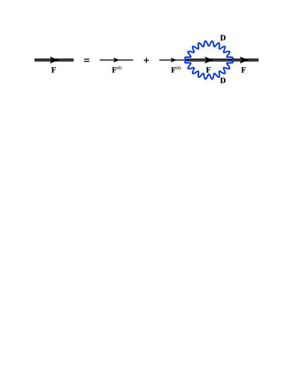
Figure 1: Feynman diagrams for the self-consistent Born approximation. Fermion (holon-doublon) and boson (magnon) propagators are represented respectively by the straight and wavy lines.

We define the full charge, or holon-doublon, Matsubara Green function as

$$\mathbf{F}(\mathbf{k},\tau)=-\langle T_{\tau}\psi_{\mathbf{k}}(\tau)\psi_{\mathbf{k}}^{{\dagger}}(0)\rangle$$ (21)

and calculate this within the SCBA. The corresponding Feynman diagrams, shown in Fig. 1, are the bare term, $\mathbf{F}^{(0)}$, and the first loop, in which the magnon Green function is also a $2\times 2$ matrix,

$$D(\mathbf{k},\tau)\!=\!-\!\left(\!\!\begin{array}[]{cc}\langle T_{\tau}s_{\mathbf{k,\uparrow}}(\tau)s_{\mathbf{k,\uparrow}}^{{\dagger}}(0)\rangle&\langle T_{\tau}s_{-\mathbf{k,\downarrow}}^{{\dagger}}(\tau)s_{\mathbf{k,\uparrow}}^{{\dagger}}(0)\rangle\!\\ \langle T_{\tau}s_{\mathbf{k,\uparrow}}(\tau)s_{-\mathbf{k,\downarrow}}(0)\rangle&\langle T_{\tau}s_{-\mathbf{k,\downarrow}}^{{\dagger}}(\tau)s_{-\mathbf{k,\downarrow}}(0)\rangle\end{array}\!\!\right)\!.$$

At this level we obtain the self-consistent Dyson equation for the Matsubara Green function of the charge sector,

$$\mathbf{F}(\mathbf{k},i\omega_{n})=\frac{1}{i\omega_{n}-\tilde{\varepsilon}_{\mathbf{k}}-\mathbf{\Sigma}(\mathbf{k},i\omega_{n})},$$ (22)

whence the retarded Green function is obtained by the analytic continuation $i\omega_{n}\rightarrow\omega+i\eta$. This $\eta$ term denotes a broadening of the peaks in the spectral response and is set to $\eta=0.1$ throughout our calculations; a smaller value would be of little physical meaning because of the finite system sizes in the calculations to follow.

We comment that, despite the simplicity of the AFM Heisenberg model, there is no exact solution for the $S=1/2$ case on the square lattice Manousakis-1991 . The study of the two-dimensional (2D) quantum AFM Heisenberg model is of great importance in its own right as a fundamental problem in quantum magnetism. To date, the most definitive analytical results for the low-temperature regime were obtained by two-loop renormalization-group calculations on the quantum nonlinear $\sigma$ model (NL$\sigma$M) Chakravarty-1989 . It has also been shown Schulz-1990 ; Dupuis-2004 that spin fluctuations in the 2D Hubbard model at low temperature can be described by the quantum NL$\sigma$M for any value of the Coulomb repulsion, $U$. The accuracy of these results notwithstanding, an integration of the NL$\sigma$M into the present analysis is not straightforward, and we will show that the holon-doublon framework with mean-field decoupling is already sufficient to gain semi-quantitative accuracy.

III Benchmarking SCBA: Quantum Monte Carlo

We investigate the half-filled 2D Hubbard model by determinantal QMC. The quartic term in Eq. (1), $U(n_{i\uparrow}-{\textstyle\frac{1}{2}})(n_{i\downarrow}-{\textstyle\frac{1}{2}})$, is decoupled by Hubbard-Stratonovich transformation to a form quadratic in $(n_{i\uparrow}-n_{i\downarrow})=(c^{\dagger}_{i\uparrow}c_{i\uparrow}-c^{\dagger}_{i\downarrow}c_{i\downarrow})$ BSS-1981 ; Hirsch-1983 ; Hirsch-1985 , which introduces an auxiliary Ising field on each lattice site. The QMC procedure obtains the partition function of the underlying Hamiltonian in a path-integral formulation in a space of dimension $N=L\times L$ and an imaginary time $\tau$ up to $\beta=1/T$. All of the physical observables are measured from the ensemble average over the space-time ($N\beta$) configurational weights of the auxiliary fields. As a consequence, the errors within the process are well controlled; specifically, the $(\Delta\tau)^{2}$ systematic error from the imaginary-time discretization, $\Delta\tau=\beta/M$, is controlled by the extrapolation $M\to\infty$ and the statistical error is controlled by the central-limit theorem (simply put, the larger the number of QMC measurements, the smaller the statistical error).

The QMC algorithm is based on Ref. BSS-1981 and has been refined by including global moves Scalettar-1991 to improve ergodicity and delay updating of the fermion Green function, which increases the efficiency of the QMC sampling. Details concerning the QMC simulation code are provided in Ref. quest . We have performed simulations for system sizes $L=4$, 8, 10, 12, 14, and 16. The interaction, $U$, is varied from $2$ to $12$ in units of the hopping strength, which is set to $t=1$, and for each $U$ we simulate temperatures from $T=0.0625$ to $1$ (inverse temperatures $\beta=1$ to $16$).

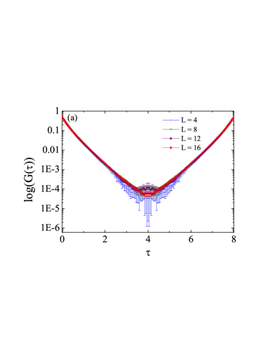
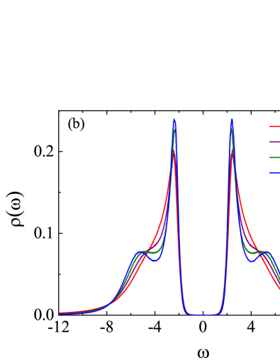
Figure 2: QMC and analytic continuation at low temperatures: (a) imaginary-time Green function, $G_{ii}(\tau)=\frac{1}{N}\sum_{\mathbf{k}\in\text{BZ}}G_{\sigma}(\mathbf{k},\tau)$, at $U=8$ and $\beta=8$ ($T=0.125$) for $L=4,\dots,16$. The logarithmic $y$-axis makes clear that $L=8$, $12$, and $16$ give the same slope in the imaginary-time decay, which ensures high-quality results on analytic continuation. (b) Local density of states, $\rho(\omega)$, obtained from SAC of the imaginary-time Green function in panel (a). Results in the gap region have clearly converged for $L=8$, $12$, and $16$ at this temperature.

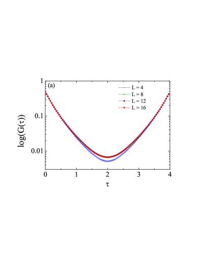
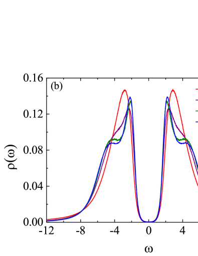
Figure 3: QMC and analytic continuation at high temperatures: (a) imaginary-time Green function, $G_{ii}(\tau)=\frac{1}{N}\sum_{\mathbf{k}\in\text{BZ}}G_{\sigma}(\mathbf{k},\tau)$, at $U=8$ and $\beta=4$ ($T=0.25$) for $L=4,\dots,16$. Again the $L=8$, $12$, and $16$ data provide converged values for the imaginary-time decay, but an exponential form is no longer clear. (b) Local density of states, $\rho(\omega)$, obtained from SAC of the imaginary-time Green function in panel (a). The gap no longer follows a single-exponential form, making it difficult to extract a reliable value of $\Delta_{\text{Mott}}$ at this temperature.

The QMC simulations give direct access to the imaginary-time fermion Green function

$$G_{\sigma}(\mathbf{k},\tau)=-\frac{1}{N}\sum_{i,j}e^{i\mathbf{k}\cdot(\mathbf{r}_{i}-\mathbf{r}_{j})}\langle c_{i\sigma}(\tau)c_{j\sigma}^{{\dagger}}(0)\rangle,$$ (23)

where $i,j\in[1,N]$ are site labels, $\tau\in[0,\beta]$ is the imaginary time, and $\langle\dots\rangle$ is the Monte Carlo expectation value. Concerning the spin index, $\sigma$, in the half-filled Hubbard model $G(\mathbf{k},\tau)=G_{\uparrow}(\mathbf{k},\tau)=G_{\downarrow}(\mathbf{k},\tau)$. While the slave-fermion treatment of Sec. II offers a specific calculation based on certain uncontrolled (but demonstrably justified) approximations, the quantity $G(\mathbf{k},\tau)$ obtained from QMC is exact on a finite-size system and has controlled errors.

To obtain real-frequency data, it is necessary to perform analytic continuation of the imaginary-time data. For this purpose we have employed stochastic analytic continuation (SAC) Beach-2004 ; Sandvik2016 , by which the spectral function, $A(\mathbf{k},\omega)$, is obtained from the Green function, $G(\mathbf{k},\tau)$, by a stochastic inverse Laplace transformation,

$$G(\mathbf{k},\tau)=\int d\omega\frac{e^{-\omega\tau}}{e^{-\beta\omega}+1}A(\mathbf{k},\omega).$$ (24)

The most recent implementation of the SAC method reproduces the spectral function using a large number of $\delta$-functions sampled at locations in a frequency continuum and collected in a histogram Sandvik2016 ; YQQin2017 ; HShao2017 . From the spectral function it is straightforward to obtain the local density of states, $\rho(\omega)=\int_{\mathbf{k}\in\text{BZ}}d\mathbf{k}A(\mathbf{k},\omega)$. Other static physical observables, such as the average double site occupancy, $D=\frac{1}{N}\sum_{i}\langle n_{i\uparrow}n_{i\downarrow}\rangle$, are also measured readily in QMC.

To access the single-particle gap, i.e. the Mott gap ($\Delta_{\text{Mott}}$) in what follows, one may attempt to read it directly from the gap in $\rho(\omega)$. From the robust exponential decay of $G_{ii}(\tau)$ in imaginary time at lower temperatures, shown for $\beta=8$ in Fig. 2(a), the analytic continuation is straightforward and yields high-quality results for $\rho(\omega)$ [Fig. 2(b)]. We find in this temperature regime that the density of states is well characterized by a single gap, $\Delta_{\text{Mott}}=3.2(3)$. However, it becomes more difficult to extract an accurate value for the Mott gap as the temperature increases. Figure 3 shows $G_{ii}(\tau)$ and $\rho(\omega)$ at $U=8$ but for $\beta=4$ ($T=0.25$). Although the imaginary-time decay of $G_{ii}(\tau)$ has converged for $L=8$, $12$, and $16$ [Fig. 3(a)], the finite-$T$ broadening that affects the Green function around $\tau=\beta/2$ makes the fit to an exponential decay less accurate. From $\rho(\omega)$ [Fig. 3(b)], it remains clear at a qualitative level that the spectrum has a gap, and that simulations for $L=8$, $12$, and $16$ converge to the same curve, but it is no longer clear how to ascribe this behavior to a specific value of $\Delta_{\text{Mott}}$. We discuss systematic ways of extracting lower and upper bounds on the Mott gap from $\rho(\omega)$ in Sec. IVC.

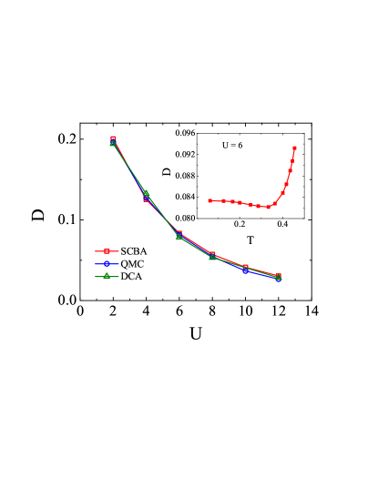
Figure 4: Double occupancy, $D$, calculated as a function of $U$ at $T=0.125$. SCBA (red) and QMC (blue) results for 16$\times$16 systems are compared with infinite-system results extrapolated from the dynamical cluster approximation (DCA) LeBlanc-2015 (green). Inset: $D(T)$ at $U=6$ from SCBA.

For a quantitative benchmarking of our SCBA results, we apply both methods on systems of size 16$\times$16. Figure 4 shows the $U$-dependence of the double occupancy at a temperature $T=0.125$. $D$ reflects the extent of charge fluctuations due to quantum and thermal effects. $D$ is suppressed as $U$ increases, and we find excellent (percent-level) agreement of SCBA and QMC. Also shown in Fig. 4 are extrapolated DCA results LeBlanc-2015 , which confirm not only the SCBA and QMC results but also their convergence to the thermodynamic limit. The inset of Fig. 4 shows $D(T)$ computed at fixed $U=6$. The weak dip is a sensitive feature that has been the subject of extensive debate Georges-1993 ; Werner-2005 ; Thereza-2010 ; Gorelik-2010 ; Imada-2016 . Our slave-fermion approach provides a straightforward understanding of possible nonmonotonic behavior in terms of the competition between weakening spin-fluctuation-induced holon-doublon stabilization and strengthening thermal fluctuations.

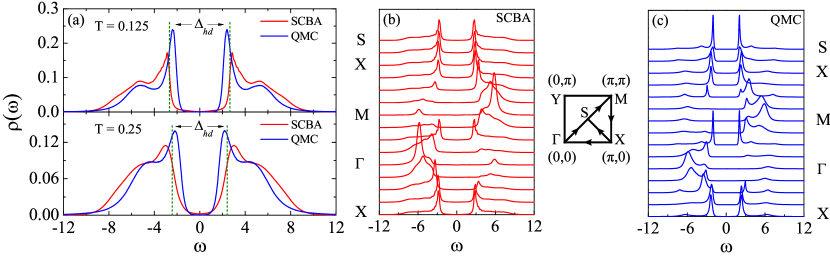
Figure 5: (a) Electronic d.o.s., $\rho(\omega)$, computed for $U=8$ by SCBA (red) and QMC (blue) for $T=0.125$ (upper panel) and $T=0.25$ (lower). Green dashed lines indicate the holon-doublon gap. (b) Spectral function, $A(\mathbf{k},\omega)$, for $U=8$ and $T=0.125$, computed by SCBA and (c) by QMC. (d) Path $\text{X}\rightarrow\Gamma\rightarrow\text{M}\rightarrow\text{X}\rightarrow\text{S}$ of high-symmetry directions in the Brillouin zone.

In the slave-fermion framework, the electron Green function, $G(\mathbf{k},i\omega_{n})$, is the convolution of the charge (holon-doublon) and spin propagators. Its calculation gives direct access to the electron spectral function, $A(\mathbf{k},\omega)=-\frac{1}{\pi}\text{Im}\,G^{R}(\mathbf{k},\omega+i\eta)$, and the density of states (d.o.s.), $\rho(\omega)=\frac{1}{N}\sum_{\mathbf{k}}A(\mathbf{k},\omega)$. Figure 5(a) shows the SCBA and QMC d.o.s. for $U=8$ at $T=0.125$ and 0.25. Three features are evident immediately. (i) Despite the absence of AFM order, $\rho(\omega)$ shows a clear Mott (single-particle) gap. $\Delta_{\text{Mott}}$, marking a region of strongly suppressed d.o.s., survives to $T>0.25$, its decrease with $T$ signaling a “melting” of the Mott insulator. (ii) The sharp peak at the Hubbard-band edge indicates the emergence of a well-defined quasiparticle due to mutual charge and spin renormalization. Following the discussion of a hole moving in an ordered AFM Rink-1988 ; Kane-1989 ; Martinez-1991 , we name this feature a “generalized spin polaron” and find that it loses coherence (as thermal fluctuations exceed spin fluctuations) towards $T=0.25$. (iii) At $T=0.125$, $\rho(\omega)$ shows an obvious peak-dip-hump structure above the Mott gap, a much-debated feature not captured in early QMC simulations Bulut-1994 but clearly reproduced here by both SCBA and QMC.

Figures 5(b) and 5(c) show respectively the SCBA and QMC spectral functions across the Brillouin zone for $U=8$. The results are again quantitatively similar in line shapes and positions, albeit with differences in peak intensities and a small but systematic discrepancy in gaps. The larger SCBA gaps may reflect an overestimate of spin-fluctuation effects at intermediate $T$ values.

Extensive calculations of the type illustrated in Figs. 4 and 5 verify that the SCBA results are completely consistent with QMC over the full range of intermediate $U$ and $T$. Thus it is safe to conclude that the holon-doublon formulation and SCBA treatment do incorporate correctly the interactions and mutual renormalization between the charge and spin sectors. Hence the qualitative physics underlying the key features of the Mott insulator, including the quasiparticle dynamics, Mott gap, and pseudogap, can finally be uncovered.

IV Convolution of Charge and Spin

More specifically, the slave-fermion framework makes it possible to separate the contributions of the charge and spin sectors to the electronic spectral function, which is a convolution of both. Figure 6 presents a schematic illustration of the situation by showing an electronic excitation in a Mott insulator. The lower and upper bands in the charge sector (red) have the holon-doublon gap, $\Delta_{\text{hd}}$. This quantity defines the high energy scale of the Mott insulator and its origin in holon-doublon binding gives it a $T$-dependence analogous to the BCS superconducting gap. In the spin sector (blue), low-energy particle-hole excitations exist over a band of width $\Omega\approx 4J$, but only those on an energy scale $\Omega(T)$, which is governed by the temperature, are activated. The electronic degrees of freedom (purple) are reconstructed as the convolution of the two sectors and hence their excitations are characterized by a gap $\Delta_{\text{Mott}}(T)\approx\Delta_{\text{hd}}(T)-2\Omega(T)$. In contrast to band insulators, where the gap is largely $T$-independent Gebhard-1997 , the Mott gap is determined by $T$-dependent correlation effects. As $T$ increases, $\Delta_{\text{Mott}}$ is driven downwards both by the decrease in $\Delta_{\text{hd}}(T)$ and by the increasing $\Omega(T)$.

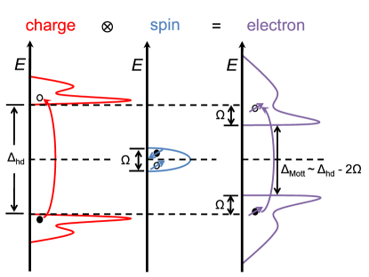
Figure 6: Schematic representation of how the Mott-insulating state of electrons (purple) is formed by convolution of the charge (red) and spin (blue) degrees of freedom.

IV.1 Charge Green function

We begin by considering the charge Green function of Eq. (22) in order to extract $\Delta_{\text{hd}}(T)$. The dispersion relation, $E_{\mathbf{k}}$, of the holon-doublon collective mode is obtained from the poles of this Green function Mahan-1990 and the holon-doublon gap is twice its minimum value, $\Delta_{\text{hd}}=2\min|_{\mathbf{k}}[|E_{\mathbf{k}}|]$. We exploit the fact that the Pauli matrices, $\sigma_{i}$ ($i=1$, 2, 3), and the identity matrix, $I$, form a complete basis for all 2$\times$2 matrices to reexpress Eq. (19) as

$$\tilde{\varepsilon}_{\mathbf{k}}={\textstyle\frac{1}{2}}U\sigma_{3}-\zeta_{\mathbf{k}}\sigma_{2},$$ (25)

where $\zeta_{\mathbf{k}}$ denotes $-8itQ\eta_{\mathbf{k}}/J$. The self-energy of the charge Green function (22) is a 2$\times$2 matrix,

$$\mathbf{\Sigma}(\mathbf{k},i\omega_{n}) = i\omega_{n}[1-Z(\mathbf{k},i\omega_{n})]I+\chi(\mathbf{k},i\omega_{n})\sigma_{3}$$ (26)

$$+\phi_{1}(\mathbf{k},i\omega_{n})\sigma_{1}+\phi_{2}(\mathbf{k},i\omega_{n})\sigma_{2},$$

in which $Z(\mathbf{k},i\omega_{n})$ is the quasiparticle renormalization factor, $\chi(\mathbf{k},i\omega_{n})$ contains the corrections to the dispersion, and the off-diagonal terms, $\phi_{1}(\mathbf{k},i\omega_{n})$ and $\phi_{2}(\mathbf{k},i\omega_{n})$, contain the effects of the binding interaction Eliashberg-1960 ; Scalapino-1966 . Substituting Eq. (26) into Eq. (22) gives

$$\mathbf{F}^{-1}(\mathbf{k},i\omega_{n})=\left(\!\!\begin{array}[]{cc}\mathbf{F}_{11}^{-}(\mathbf{k},i\omega_{n})&-\mathbf{F}_{12}^{-}(\mathbf{k},i\omega_{n})\\ -\mathbf{F}_{12}^{+}(\mathbf{k},i\omega_{n})&\mathbf{F}_{11}^{+}(\mathbf{k},i\omega_{n})\end{array}\!\!\right)\!,$$ (27)

in which

$$\mathbf{F}_{11}^{\pm}(\mathbf{k},i\omega_{n}) = Z(\mathbf{k},i\omega_{n})i\omega_{n}\pm[U/2+\chi(\mathbf{k},i\omega_{n})],$$

$$\mathbf{F}_{12}^{\pm}(\mathbf{k},i\omega_{n}) = \phi_{1}(\mathbf{k},i\omega_{n})\pm i[\phi_{2}(\mathbf{k},i\omega_{n})-\zeta_{\mathbf{k}}].$$

By inversion of the matrix we obtain

$$\mathbf{F}(\mathbf{k},i\omega_{n})=\frac{1}{|\text{DetF}|}\left(\!\!\begin{array}[]{cc}\mathbf{F}_{11}^{+}(\mathbf{k},i\omega_{n})&\mathbf{F}_{12}^{-}(\mathbf{k},i\omega_{n})\\ \mathbf{F}_{12}^{+}(\mathbf{k},i\omega_{n})&\mathbf{F}_{11}^{-}(\mathbf{k},i\omega_{n})\end{array}\!\!\right),$$ (28)

where

$$|\text{DetF}| = Z^{2}(\mathbf{k},i\omega_{n})(i\omega_{n})^{2}-[U/2+\chi(\mathbf{k},i\omega_{n})]^{2}$$ (30)

$$-\phi_{1}^{2}(\mathbf{k},i\omega_{n})-[\phi_{2}(\mathbf{k},i\omega_{n})-\zeta_{\mathbf{k}}]^{2}$$

$$= R(\mathbf{k},\omega)[\omega-E_{\mathbf{k}}+i\Gamma(\mathbf{k},\omega)]$$

$$\;\;\;\;\times[\omega+E_{\mathbf{k}}+i\Gamma(\mathbf{k},\omega)].$$

We have calculated $\mathbf{F}(\mathbf{k},i\omega_{n})$ numerically, which gives access to its component parts $Z(\mathbf{k},i\omega_{n})$, $\chi(\mathbf{k},i\omega_{n})$, $\phi_{1}(\mathbf{k},i\omega_{n})$, and $\phi_{2}(\mathbf{k},i\omega_{n})$. By reexpressing the denominator in the form given in Eq. (30), we derive the effective holon-doublon quasiparticle dispersion, $E_{\mathbf{k}}$, and the corresponding scattering rate, $\Gamma(\mathbf{k},\omega)$ Mahan-1990 . We obtain the result for $\Delta_{\text{hd}}(T)$ shown as the green curve in Fig. 7.

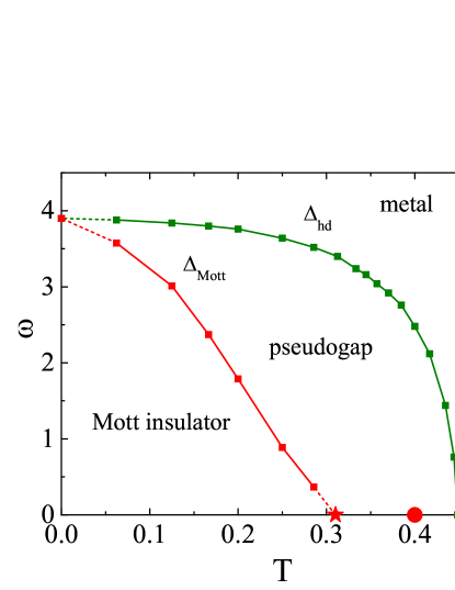
Figure 7: Temperature-dependence of the charge ($\Delta_{\text{hd}}$, green) and Mott ($\Delta_{\text{Mott}}$, red) gaps for the Hubbard model with $U=6$, estimated from the SCBA $\rho(\omega)$. Red squares indicate the lower bound on $\Delta_{\text{Mott}}$. The red star and circle mark respectively the lower and upper bounds on the temperature, $T_{c}^{\rm Mott}$, at which $\Delta_{\rm Mott}(T)$ vanishes. Dashed red lines indicate extrapolations based on our lower-bound values.

IV.2 Electron spectral function

By contrast, $\Delta_{\text{Mott}}(T)$ is the single-particle gap and is smaller than $\Delta_{\text{hd}}(T)$ due to the spin-renormalization of the charge sector [Fig. 6]. This renormalization is contained in the slave-fermion formulation within the convolution making up the electron Green function, which if vertex corrections are neglected Raimondi-1993 ; Yamaji-2011 may be expressed as

$$G_{ij}^{\sigma}(\tau) = -\langle T_{\tau}c_{i\sigma}(\tau)c_{j\sigma}^{{\dagger}}(0)\rangle$$

$$= -\langle T_{\tau}(s_{i\overline{\sigma}}^{\dagger}(\tau)d_{i}(\tau)+\sigma e_{i}^{{\dagger}}(\tau)s_{i\sigma}(\tau))$$

$$\;\;\;\;\;\;\times(d_{j}^{{\dagger}}(0)s_{j\overline{\sigma}}(0)+\sigma s_{j\sigma}^{{\dagger}}(0)e_{j}(0))\rangle$$

$$\simeq -\langle T_{\tau}d_{i}(\tau)d_{j}^{{\dagger}}(0)\rangle\langle T_{\tau}s_{i\overline{\sigma}}^{{\dagger}}(\tau)s_{j\overline{\sigma}}(0)\rangle$$

$$-\langle T_{\tau}e_{i}^{{\dagger}}(\tau)e_{j}(0)\rangle\langle T_{\tau}s_{i\sigma}(\tau)s_{j\sigma}^{{\dagger}}(0)\rangle$$

$$-\sigma\langle T_{\tau}d_{i}(\tau)e_{j}(0)\rangle\langle T_{\tau}s_{i\overline{\sigma}}^{{\dagger}}(\tau)s_{j\sigma}^{{\dagger}}(0)\rangle$$

$$-\sigma\langle T_{\tau}e_{i}^{{\dagger}}(\tau)d_{j}^{{\dagger}}(0)\rangle\langle T_{\tau}s_{i\sigma}(\tau)s_{j\overline{\sigma}}(0)\rangle.$$

In momentum space it is given by

$$G_{\sigma} (\mathbf{k},i\omega_{n})$$ (32)

$$= \;\frac{1}{N}\sum_{\mathbf{q}}\left(\int_{-\infty}^{\infty}d\varepsilon\,\frac{U_{\mathbf{q}}^{{\dagger}}\mathbf{A}(\mathbf{k+q},\varepsilon)U_{\mathbf{q}}}{i\omega_{n}+\Omega_{\mathbf{q}}-\varepsilon}\,[f(\varepsilon)+n_{\mathbf{q}}]\right.$$

$$\;\;\left.+\int_{-\infty}^{\infty}d\varepsilon\,\frac{V_{\mathbf{q}}^{{\dagger}}\mathbf{A}(\mathbf{k+q},\varepsilon)V_{\mathbf{q}}}{i\omega_{n}-\Omega_{\mathbf{q}}-\varepsilon}\,[1-f(\varepsilon)+n_{\mathbf{q}}]\right)\!,$$

with

$$U_{\mathbf{q}}=\left(\!\!\begin{array}[]{c}u_{\mathbf{q}}\\ v_{\mathbf{q}}^{\ast}\end{array}\!\!\right)\;\;\text{and}\;\;V_{\mathbf{q}}=\left(\!\!\begin{array}[]{c}v_{\mathbf{q}}\\ u_{\mathbf{q}}^{\ast}\end{array}\!\!\right)\!,$$ (33)

whose components are given in Eq. (14), and

$$\mathbf{A}(\mathbf{k+q},\varepsilon) = -\frac{1}{\pi}\text{Im}\,\mathbf{F}^{R}(\mathbf{k+q},\varepsilon+i\eta)$$ (34)

$$= \left(\!\begin{array}[]{cc}A_{11}(\mathbf{k+q},\varepsilon)&A_{12}(\mathbf{k+q},\varepsilon)\\ A_{21}(\mathbf{k+q},\varepsilon)&A_{22}(\mathbf{k+q},\varepsilon)\end{array}\!\right)\!,$$ (37)

which expresses the holon-doublon spectral function corresponding to the retarded charge Green function; $f(\varepsilon)$ is the Fermi-Dirac distribution function for holon-doublon quasiparticles and $n_{\mathbf{q}}$ the Bose-Einstein distribution for the spinons.

The corresponding electron spectral function is

$$\tilde{A}_{\sigma}(\mathbf{k},\omega)=-\frac{1}{\pi}\textrm{Im}\,G_{\sigma}^{R}(\mathbf{k},\omega)$$ (38)

$$=\;\frac{1}{N}\!\sum_{\mathbf{q}}\!\!\int_{-\infty}^{\infty}\!\!d\varepsilon U_{\mathbf{q}}^{{\dagger}}\mathbf{A}(\mathbf{k\!+\!q},\varepsilon)U_{\mathbf{q}}[f(\varepsilon)\!+\!n_{\mathbf{q}}]\delta(\omega\!+\!\Omega_{\mathbf{q}}\!-\!\varepsilon)$$

$$\!\!+\frac{1}{N}\!\sum_{\mathbf{q}}\!\!\int_{-\infty}^{\infty}\!\!\!d\varepsilon V_{\mathbf{q}}^{{\dagger}}\mathbf{A}(\mathbf{k\!+\!q},\varepsilon)V_{\mathbf{q}}[1\!-\!f(\varepsilon)\!+\!n_{\mathbf{q}}]\delta(\omega\!-\!\Omega_{\mathbf{q}}\!-\!\varepsilon),$$

whence the electronic density of states is

$$\rho(\omega) = \frac{1}{N}\sum_{\mathbf{k},\sigma}\rho_{\sigma}(\mathbf{k},\omega)$$

$$= \sum_{\mathbf{q}}a(\omega,\mathbf{q})\int_{-\infty}^{\infty}d\varepsilon\rho_{hd}^{1}(\mathbf{q},\varepsilon)\delta(\omega+\Omega_{\mathbf{q}}-\varepsilon)$$

$$+\sum_{\mathbf{q}}b(\omega,\mathbf{q})\int_{-\infty}^{\infty}d\varepsilon\rho_{hd}^{2}(\mathbf{q},\varepsilon)\delta(\omega-\Omega_{\mathbf{q}}-\varepsilon),$$

in which

$$\rho_{hd}^{1}(\mathbf{q},\varepsilon)=U_{\mathbf{q}}^{{\dagger}}\mathbf{A}_{\mathbf{q}}(\varepsilon)U_{\mathbf{q}},\;\rho_{hd}^{2}(\mathbf{q},\varepsilon)=V_{\mathbf{q}}^{{\dagger}}\mathbf{A}_{\mathbf{q}}(\varepsilon)V_{\mathbf{q}},$$

and

$$a(\omega,\mathbf{q}) = \frac{1}{N}[f(\omega+\Omega_{\mathbf{q}})+n_{\mathbf{q}}],$$

$$b(\omega,\mathbf{q}) = \frac{1}{N}[1-f(\omega-\Omega_{\mathbf{q}})+n_{\mathbf{q}}],$$

where $\Omega_{\mathbf{q}}$ is the dispersion relation of the spin excitations. The quantities $\rho_{hd}^{1}(\mathbf{q},\varepsilon)$ and $\rho_{hd}^{2}(\mathbf{q},\varepsilon)$ contain the holon-doublon density of states appearing in $\mathbf{A}_{\mathbf{q}}(\varepsilon)$, with nontrivial quantitative modification by the spin part (contained in $U_{\mathbf{q}}$ and $V_{\mathbf{q}}$). The temperature-dependence is contained within the occupation functions in $a(\omega,\mathbf{q})$ and $b(\omega,\mathbf{q})$. The renormalization of the holon-doublon gap to the Mott gap is contained within the integrals over the two energy $\delta$-functions in Eq. (IV.2), $\delta(\omega\pm\Omega_{\mathbf{q}}-\varepsilon)$, which mathematically effect the convolution with the spin spectral function at the SCBA level and physically specify how the lower and upper Hubbard bands are produced from holon-doublon bound states dressed by the emission and absorption of low-energy spin fluctuations.

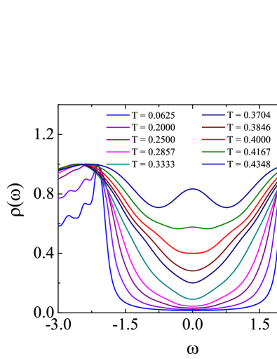
Figure 8: $\rho(\omega)$ in the gap region at all temperatures, computed from SCBA with $U=6$ and $\eta=0.1$; results are normalized to a peak height of 1 in order to highlight the emerging $\omega=0$ peak.

IV.3 Extraction of the Mott gap

Unlike $\Delta_{\text{hd}}(T)$, the accurate extraction of $\Delta_{\text{Mott}}(T)$ from the electron Green function is complicated by the lack of a single-particle dispersion relation, and hence no analytical means of finding the poles in the self-energy. However, as noted in Sec. III, it is even more difficult to read $\Delta_{\text{Mott}}$ from QMC for temperatures in excess of approximately 0.15. Thus we revert to a detailed consideration of the SCBA electronic d.o.s., $\rho(\omega,T)$ [Fig. 8], in order to estimate $\Delta_{\text{Mott}}(T)$ by a procedure of assuming an effective gap and modelling its “filling.” We apply two types of analysis to obtain (1) a lower bound on $\Delta_{\rm Mott}(T)$, using a quantitative fitting process which in essence neglects thermal fluctuations, and (2) an upper bound on the temperature, $T_{c}^{\rm Mott}$, at which $\Delta_{\rm Mott}(T)=0$, based on a clear qualitative feature of $\rho(\omega,T)$.

IV.3.1 Lower bound on $\Delta_{\rm Mott}(T)$

Except at the highest temperatures, all of the d.o.s. functions we calculate by SCBA show the clear presence of a gap which, however, is partially filled. This finite d.o.s. at small $\omega$ is a consequence of two effects, the (finite-size) Lorentzian broadening, $\eta$, and the temperature, whose effects appear as exponential activation over an effective $T$-dependent gap. A qualitative indication of the differing nature of the two contributions can be obtained by comparing $\rho(\omega,T)$ from SCBA, shown in Fig. 8, with the results from QMC, which we show in Fig. 9: $\eta$ effects, which cause $\rho(\omega)$ to become more “V-shaped” within the gap, are stronger in the SCBA data. However, we are constrained by finite-size effects not to reduce $\eta$ in our calculations. Because the Lorentzian contribution is much stronger, we proceed by neglecting the thermal activation contribution, i.e. the direct effects of $T$, and thus obtain a lower bound for $\Delta_{\text{Mott}}(T)$. Thus the problem of finding the Mott gap, meaning the gap in the reconstructed (spin-charge-recombined) spectrum at any given $T$, is reduced to a deconvolution removing $\eta$.

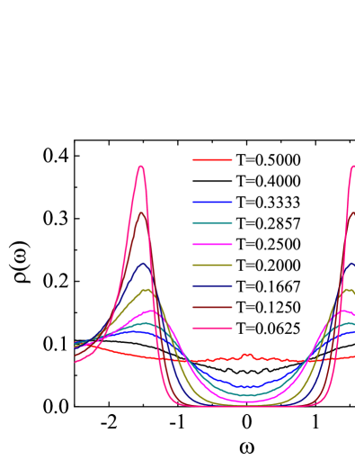
Figure 9: $\rho(\omega)$ in the gap region for a number of temperature values, computed by QMC with $U=6$.

The retarded Green function can be represented by

$$G^{R}(\omega+i\eta)=\int_{-\infty}^{\infty}d\varepsilon\,\frac{{\tilde{\rho}}(\varepsilon)}{\omega-\varepsilon+i\eta},$$ (40)

where ${\tilde{\rho}}(\varepsilon)$, the intrinsic d.o.s., is expected to vanish below $\Delta_{\text{Mott}}/2$. We need consider only the imaginary part of $G^{R}(\omega+i\eta)$, which is the observed d.o.s.,

$$\rho(\omega)=\frac{1}{\pi}\int_{-\infty}^{\infty}d\varepsilon\,\frac{\eta}{(\omega-\varepsilon)^{2}+\eta^{2}}\,{\tilde{\rho}}(\varepsilon).$$ (41)

If $\eta$ is infinitesimal, at $T=0$ and when the energy interval is continuous one has ${\tilde{\rho}}(\omega)=\rho(\omega)$. In our calculations, however, $\eta$ is finite and we have used an energy interval $d\omega=0.02$, on top of which we wish to demonstrate that the effect of finite temperatures on the spectral function is equivalent to that of a $T$-dependent effective Mott gap, $\Delta_{\rm Mott}(T)$.

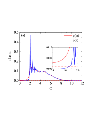
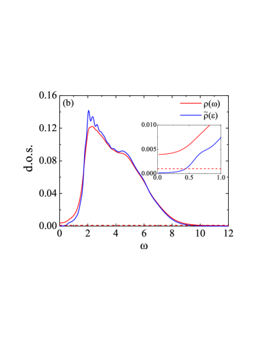
Figure 10: Deconvolution of Lorentzian broadening in the SCBA d.o.s. (a) Comparison of the functions $\rho(\omega)$, calculated by SCBA, and $\tilde{\rho}(\varepsilon)$, obtained from it by linear regression, for $U=6$ at temperature $T=0.125$. (b) The same comparison at $T=0.25$. Clearly $\tilde{\rho}(\varepsilon)$ reveals additional intrinsic features of the spectral function by removing the Lorentzian broadening, and hence allows an estimate of $\Delta_{\text{Mott}}$. We comment that the SCBA data for $\rho(\omega)$ contain $N_{\omega}=600$ frequency points and the linear regression is performed to obtain a dataset $\tilde{\rho}(\varepsilon)$ containing $N_{\varepsilon}=300$ points. The dashed lines show the criterion $\tilde{\rho}(\varepsilon)<0.001$, on the basis of which we take the spectral weight to vanish and thus define $\Delta_{\text{Mott}}$.

As noted above, for a Mott insulator with no thermal fluctuations, one expects that ${\tilde{\rho}}(\omega)=0$ in the energy interval $[-\Delta_{\rm Mott}/2,\Delta_{\rm Mott}/2]$, whence

$$\rho(\omega)=\frac{2}{\pi}\int_{\Delta_{\rm Mott}/2}^{\infty}d\varepsilon\,\frac{\eta}{(\omega-\varepsilon)^{2}+\eta^{2}}\,{\tilde{\rho}}(\varepsilon).$$ (42)

The process of using $\rho(\omega)$, as calculated by SCBA at each value of $T$, to extract the underlying function ${\tilde{\rho}}(\varepsilon)$ and the single constant $\Delta_{\rm Mott}(T)$ is analogous to an analytic continuation. Although a full SAC treatment of the SCBA data is complicated by a lack of statistical errors, a more straightforward procedure is sufficient in the present case. Borrowing from the structure of the SAC method of Sec. III, we construct a minimization based on linear regression to achieve the decomposition of Eq. (42). We parameterize

$$\tilde{\rho}(\varepsilon)=\sum^{N_{\epsilon}}_{i=1}a_{i}\delta(\varepsilon-\varepsilon_{i})$$ (43)

using $N_{\varepsilon}$ equally spaced $\delta$-functions, whose weights $\{a_{i}\}$ are the free parameters. By inserting Eq. (43) into Eq. (42), we obtain the function

$$\rho^{\prime}(\omega)=\frac{1}{\pi}\sum^{N_{\epsilon}}_{i=1}d\varepsilon\left[\frac{\eta}{(\omega-\varepsilon_{i})^{2}+\eta^{2}}+\frac{\eta}{(\omega+\varepsilon_{i})^{2}+\eta^{2}}\right]\,a_{i},$$ (44)

by which we approximate the SCBA $\rho(\omega)$. We define the goodness-of-fit parameter

$$\chi^{2}=\sum_{i=1}^{N_{\omega}}\big{(}\rho(\omega_{i})-\rho^{\prime}(\omega_{i})\big{)}^{2},$$ (45)

whose minimization by a linear regression method determines the values $\{a_{i}\}$. Because the number, $N_{\varepsilon}$, of data points in $\varepsilon$ in Eq. (43) can only be equal to or smaller than the number, $N_{\omega}=600$, of points in the SCBA $\rho(\omega)$, such a minimization can always be achieved.

Two examples of the intrinsic d.o.s. functions, $\tilde{\rho}(\varepsilon)$, underlying our computed SCBA functions, $\rho(\omega)$, are shown in Fig. 10, where we have chosen $U=6$ and the temperatures $T=0.125$ [Fig. 10(a)] and $T=0.25$ [Fig. 10(b)]; in both cases we used $N_{\varepsilon}=300$. The $\tilde{\rho}(\varepsilon)$ functions show a clear suppression of the d.o.s. at low frequencies, with the reappearance of this weight occurring primarily around the peaks. These intrinsic functions also show the clear presence of additional states building systematically into the zero-temperature gap as $T$ is increased.

To extract the effective Mott gap from $\tilde{\rho}(\varepsilon)$ at each temperature, we define $\Delta_{\mathrm{Mott}}(T)$ as the frequency at which the weights $a_{i}$ in ${\tilde{\rho}}(\varepsilon)$ start to rise from zero. More precisely, we use the criterion that $a_{i}$ should be less than 1% of the average d.o.s. at the band center, $\rho(\omega)\approx 0.1$, i.e. $a_{i}<0.001$. As shown in the insets of Figs. 10(a) and 10(b), this criterion appears to offer a reliable means of distinguishing real reconstructed finite-$T$ features from thermal and numerical noise.

By applying these considerations at $U=6$, we obtain the data shown in Fig. 7, with a well-defined lower bound from $T=0.0625$ to $T=0.2857$. At our next higher temperature, $T=0.333$, $a_{i}>0.001$ even at $\omega=0$, and thus the lower bound has become zero; we estimate the temperature at which this occurs to be $T\approx 0.31$, and represent this by the dashed line in Fig. 7. We conclude that these results can be taken to provide an accurate lower bound for $\Delta_{\rm Mott}(T)$, and that the closing of the Mott gap by this estimate provides the lower bound, $T_{c,l}^{\rm Mott}\approx 0.31$, for the associated temperature.

IV.3.2 Upper bound on $T_{c}^{\rm Mott}$

A qualitatively different approach to the Mott transition is provided by the fact that, as Figs. 8 (SCBA) and 9 (QMC) make clear, $\rho(\omega)$ changes from a low-$T$ form with an absolute minimum at $\omega=0$ to a high-$T$ form with a peak at $\omega=0$. This peak grows in size and spectral weight as a function of temperature beyond a given $T$ value. The emergence of this quasiparticle peak in the single-particle response indicates unambiguously that the lower and upper Hubbard bands have overlapped, and thus that the Mott gap has closed. In practice, $\Delta_{\text{Mott}}$ may have vanished before the peak can emerge as a feature stronger than the d.o.s. at neighboring nonzero frequencies, and hence this temperature, $T_{c,u}^{\rm Mott}$, can be taken as an upper bound for the closing of the Mott gap. At $U=6$ we find, as shown in Fig. 7, that $T_{c,u}^{\rm Mott}\approx 0.4$. Thus both $T_{c,l}^{\rm Mott}$ and $T_{c,u}^{\rm Mott}$ lie well below the closing temperature of the holon-doublon gap, $T^{\text{hd}}_{c}\simeq 0.45$. While the QMC results differ from SCBA in quantitative details, the qualitative picture of the two gaps remains robust.

V Interpretation

The $\omega=0$ axis of Fig. 7 can be interpreted as a finite-temperature phase diagram for the Hubbard model (1). The low-$T$ regime is fully gapped, not only for bound holons and doublons but also for electrons, and this is the Mott insulator. As $T$ is increased, its melting is revealed as a two-step process. At $T_{c}^{\text{Mott}}$, the optimal electronic states created by spin-charge reconstruction, which lie in the low-energy tails of the Hubbard bands, have touched, creating the $\omega=0$ peak in $\rho(\omega)$ [Fig. 8]. However, $\Delta_{\text{hd}}(T)$ remains finite and most electronic states remain gapped; the consequent suppression of the d.o.s. around the Fermi level makes this a pseudogap regime. As $T$ approaches $T_{c}^{\text{hd}}$, the pseudogap fills in with additional low-lying electronic states, and only above $T_{c}^{\text{hd}}$ does the closing of the charge gap make the system fully metallic.

This pseudogap behavior White-1993 is observed consistently in many numerical studies of the Hubbard model LeBlanc-2015 , including our own (Secs. III and IVC), and is not restricted to finite doping. The slave-fermion framework captures this phenomenon, showing how the single-particle gap decreases faster than the charge gap before the vanishing of both quantities establishes the two characteristic temperatures, $T_{c}^{\rm Mott}$ and $T_{c}^{\rm hd}$ [Fig. 7]. Even at low $T$, the difference between $\Delta_{\text{hd}}$ and $\Delta_{\text{Mott}}$ grows linearly with $T$, as anticipated in Sec. IV. This difference in the $T$-dependences of the two gaps constitutes one crucial feature of the distinctive low-energy physics intrinsic to the Mott insulator.

A further piece of essential physics concerns the energy scales of the spin fluctuations and gap renormalization. Energies in the spin sector are controlled by $J$, and the relevant temperatures for a finite (two-spin) magnetic correlation parameter are a fraction of this. However, charge-sector energies are of order $U$, and the renormalization, $\Omega(T)$, of $\Delta_{\text{hd}}(T)$ is a fraction of this. From Fig. 7, $\Omega(T)\approx 5T\approx UT$. This remarkable “leverage effect,” by which the low-energy spin processes bring about high energy shifts in the charge processes, lies at the heart of the energy-scale mixing in the Mott insulator.

Equations (IV.2) quantify how effectively the spin part modifies the filling of the charge gap during the reconstruction of the electronic degrees of freedom, and as such the leverage effect is not a directly modified energy scale, but rather a strong amplification of the gap-filling. When this process is modeled as a thermal filling governed by an effective (Mott) gap for the electrons (Sec. IVC), one finds the factor of order $U$ that enters in the difference from the charge gap. Thus the mixing of energy scales intrinsic to the Mott insulator is revealed from a set of equations affording physical insight, rather than “only” as the output from a complex numerical simulation.

These same equations also provide a quantitative description of the spectral weight in the pseudogap regime. Although the presence of particularly low-lying reconstructed electronic states has already closed the Mott gap, these states constitute only a small fraction of the total available electronic states, the majority of which still reside above the charge gap. As a consequence, the electronic d.o.s. in the low-energy regime remains suppressed, which is the definition of the pseudogap, and this suppression persists until the temperature is high enough to close the charge gap. We comment that, as in Ref. Han-2016 , the electronic Green function may also be used to obtain the Luttinger surface for the insulating regime and the Fermi surface of the pseudogap and metallic states; however, because the model we consider is half-filled and has no extended hopping, this surface is precisely the Umklapp surface (the locus of solutions of $\cos k_{x}+\cos k_{y}=0$) for all temperatures.

VI Concluding remarks

To place our results in context, all slave-particle decompositions involve an uncontrolled assumption, which is justified post facto. Our QMC simulations reveal that the holon-doublon approach does an excellent job of representing the relevant degrees of freedom and of capturing all the important aspects of their interactions. Further, any mean-field treatment enforces the local constraint only on average, making its results critically dependent on how well the essential physics is captured at lowest order. Again the holon-doublon framework passes this test with distinction, for all values of $U>2t$ [Fig. 4] and temperatures $T\lesssim 0.5J$. Unlike some approaches, our study is general in that the finite-$T$ response contains no potential pathologies induced by the perfectly nested noninteracting band.

Experimentally, despite intensive interest in cuprate materials and Mott physics, detailed studies of undoped Mott insulators are complicated in that neither angle-resolved photoemission spectroscopy (ARPES) nor scanning tunnelling spectroscopy (STS) can obtain a signal from a well-gapped insulator at low $T$. ARPES on insulating cuprates Damascelli-2003 has mapped the spectral function [Fig. 5(b)] to observe the Mott gap and strongly renormalized bands, but lack the resolution and temperature-sensitivity to address the filling and closing of $\Delta_{\text{Mott}}$. STS measures the local d.o.s. [Fig. 5(a)] and recent studies rw1 ; rw2 have observed the Mott gap and its persistence to finite temperatures, albeit in systems that are already lightly hole-doped (which is the next challenge for the slave-fermion description). Very recently, AFM order has been observed in ultracold ⁶Li atoms on an optical lattice, which also realize an undoped Hubbard model at finite temperatures rca . Given the finite nature (of order 100 atoms) of these systems, our SCBA and QMC techniques are both perfectly suited for calculations and quantitative comparison with this type of experiment.

In summary, we have shown by analytical SCBA calculations and unbiased QMC simulations that the slave-fermion description of the Hubbard model contains all the essential physics of the Mott insulator. Thus we obtain complete insight into the underlying physical processes, which emerge from high-energy holon-doublon binding mediated by low-energy, short-ranged spin fluctuations. The spin-renormalization of the charge sector, which forms the lower and upper Hubbard (electron) bands, introduces a strong energetic leverage effect. The Mott gap is smaller than the charge gap and its closure involves only a fraction of the reconstructed states, giving a natural explanation of the pseudogap. This unified understanding of the dynamics and melting of the undoped Mott insulator forms a sound basis for investigating both the doped case and specific cuprate band structures.

- (1) N. F. Mott and R. Peierls, Proc. Phys. Soc. London 49, 72 (1937).
- (2) N. F. Mott, Proc. Phys. Soc., London, Sect. A 62, 416 (1949).
- (3) N. F. Mott, Can. J. Phys. 34, 1356 (1956).
- (4) M. Imada, A. Fujimori, and Y. Tokura, Rev. Mod. Phys. 70, 1039 (1998).
- (5) J. G. Bednorz and K. A. Müller, Z. Phys. B: Condens. Matter 64, 189 (1986).
- (6) P. A. Lee, N. Nagaosa, and X.-G. Wen, Rev. Mod. Phys. 78, 17 (2006).
- (7) A. Damascelli, Z. Hussain, and Z.-X. Shen, Rev. Mod. Phys. 75, 473 (2003).
- (8) M. R. Norman, D. Pines, and C. Kallin, Adv. Phys. 54, 715 (2005).
- (9) S. Hufner, M. A. Hossain, A. Damascelli, and G. A. Sawatzky, Rep. Prog. Phys. 71, 062501 (2008).
- (10) N. F. Mott, Metal-Insulator Transitions (Taylor and Francis, London, 1990).
- (11) J. Hubbard, Proc. Roy. Soc. London, Ser. A 276, 238 (1963).
- (12) W. F. Brinkman and T. M. Rice, Phys. Rev. B 2, 4302 (1970).
- (13) C. Huscroft, M. Jarrell, Th. Maier, S. Moukouri, and A. N. Tahvildarzadeh, Phys. Rev. Lett. 86, 139 (2001).
- (14) S. Moukouri and M. Jarrell, Phys. Rev. Lett. 87, 167010 (2001).
- (15) B. Kyung, S. S. Kancharla, D. Sénéchal, A.-M. S. Tremblay, M. Civelli, and G. Kotliar, Phys. Rev. B 73, 165114 (2006).
- (16) H. Park, K. Haule, and G. Kotliar, Phys. Rev. Lett. 101, 186403 (2008).
- (17) G. Sordi, K. Haule, and A.-M. S. Tremblay, Phys. Rev. Lett. 104, 226402 (2010).
- (18) O. Gunnarsson, T. Schäfer, J. P. F. LeBlanc, E. Gull, J. Merino, G. Sangiovanni, G. Rohringer, and A. Toschi, Phys. Rev. Lett. 114, 236402 (2015).
- (19) C. Castellani, C. Di Castro, D. Feinberg, and J. Ranninger, Phys. Rev. Lett. 43, 1957 (1979).
- (20) T. A. Kaplan, P. Horsch, and P. Fulde, Phys. Rev. Lett. 49, 889 (1982).
- (21) M. Capello, F. Becca, M. Fabrizio, S. Sorella, and E. Tosatti, Phys. Rev. Lett. 94, 026406 (2005).
- (22) H. Yokoyama, M. Ogata, and Y. Tanaka, J. Phys. Soc. Jpn. 75, 114706 (2006).
- (23) P. Phillips, Rev. Mod. Phys. 82, 1719 (2010).
- (24) S. Zhou, Y. Wang, and Z. Wang, Phys. Rev. B 89, 195119 (2014).
- (25) P. Prelovšek, J. Kokalj, Z. Lenarčič, and R. H. McKenzie, Phys. Rev. B 92, 235155 (2015).
- (26) X.-J. Han, Y. Liu, Z.-Y. Liu, X. Li, J. Chen, H.-J. Liao, Z.-Y. Xie, B. Normand, and T. Xiang, New J. Phys. 18, 103004 (2016).
- (27) G. Kotliar and A. E. Ruckenstein, Phys. Rev. Lett. 57, 1362 (1986).
- (28) J. P. F. LeBlanc, A. E. Antipov, F. Becca, I. W. Bulik, G. K.-L. Chan, C.-M. Chung, Y. Deng, M. Ferrero, T. M. Henderson, C. A. Jiménez-Hoyos, E. Kozik, X.-W. Liu, A. J. Millis, N. V. Prokof’ev, M. Qin, G. E. Scuseria, H. Shi, B. V. Svistunov, L. F. Tocchio, I. S. Tupitsyn, S. R. White, S. Zhang, B.-X. Zheng, Z. Zhu, and E. Gull, Phys. Rev. X. 5, 041041 (2015), and references therein.
- (29) A. Auerbach, Interacting Electrons and Quantum Magnetism (Springer-Verlag, New York, 1994).
- (30) D. P. Arovas and A. Auerbach, Phys. Rev. B 38, 316 (1988).
- (31) D. Yoshioka, J. Phys. Soc. Jpn. 58, 1516 (1989).
- (32) W. Wu, M. S. Scheurer, S. Chatterjee, S. Sachdev, A. Georges, and M. Ferrero, Phys. Rev. X 8, 021048 (2018).
- (33) M. S. Scheurer, S. Chatterjee, W. Wu, M. Ferrero, A. Georges, and S. Sachdev, Proc. Natl. Acad. Sci. USA 115, E3665 (2018).
- (34) E. Manousakis, Rev. Mod. Phys. 63, 1 (1991).
- (35) S. Chakravarty, B. I. Halperin, and D. R. Nelson, Phys. Rev. B 39, 2344 (1989).
- (36) H. J. Schulz, Phys. Rev. Lett. 65, 2462 (1990).
- (37) K. Borejsza and N. Dupuis, Phys. Rev. B 69, 085119 (2004).
- (38) R. Blankenbecler, D. J. Scalapino, and R. L. Sugar, Phys. Rev. D 24, 2278 (1981).
- (39) J. E. Hirsch, Phys. Rev. B 28, 4059(R) (1983).
- (40) J. E. Hirsch, Phys. Rev. B 31, 4403 (1985).
- (41) R. T. Scalettar, R. M. Noack, and R. R. P. Singh, Phys. Rev. B 44, 10502 (1991).
- (42) The finite-temperature QMC simulation code is based on the Quantum Electron Simulation Toolbox (QUEST), which is a FORTRAN 90/95 package containing modern algorithms, such as delayed updating, and integrating the latest BLAS/LAPACK numerical kernels. QUEST has integrated several legacy codes by modularizing their computational components for ease of maintenance and program interfacing. The current version can be accessed at https://code.google.com/archive/p/quest-qmc/.
- (43) K. S. D. Beach, unpublished (arXiv:cond-mat/0403055).
- (44) A. W. Sandvik, Phys. Rev. E 94, 063308 (2016).
- (45) Y. Q. Qin, B. Normand, A. W. Sandvik, and Z. Y. Meng, Phys. Rev. Lett. 118, 147207 (2017).
- (46) H. Shao, Y. Q. Qin, S. Capponi, S. Chesi, Z. Y. Meng, and A. W. Sandvik, Phys. Rev. X 7, 041072 (2017).
- (47) A. Georges and W. Krauth, Phys. Rev. B 48, 7167 (1993).
- (48) F. Werner, O. Parcollet, A. Georges, and S. R. Hassan, Phys. Rev. Lett. 95, 056401 (2005).
- (49) T. Paiva, R. Scalettar, M. Randeria, and N. Trivedi, Phys. Rev. Lett. 104, 066406 (2010).
- (50) E. V. Gorelik, I. Titvinidze, W. Hofstetter, M. Snoek, and N. Blümer, Phys. Rev. Lett. 105, 065301 (2010).
- (51) K. Takai, K. Ido, T. Misawa, Y. Yamaji, and M. Imada, J. Phys. Soc. Jpn. 85, 034601 (2016).
- (52) S. Schmitt-Rink, C. M. Varma, and A. E. Ruckenstein, Phys. Rev. Lett. 60, 2793 (1988).
- (53) C. L. Kane, P. A. Lee, and N. Read, Phys. Rev. B 39, 6880 (1989).
- (54) G. Martinez and P. Horsch, Phys. Rev. B 44, 317 (1991).
- (55) N. Bulut, D. J. Scalapino, and S. R. White, Phys. Rev. Lett. 73, 748 (1994).
- (56) F. Gebhard, The Mott metal-insulator transition: Models and methods (Springer, Berlin, 1997).
- (57) G. D. Mahan, Many-Particle Physics (Plenum Press, New York, 1990).
- (58) G. M. Eliashberg, Sov. Phys. JETP 11, 696 (1960).
- (59) D. J. Scalapino, J. R. Schrieffer, and J. W. Wilkins, Phys. Rev 148, 263 (1966).
- (60) R. Raimondi and C. Castellani, Phys. Rev. B 48, 11453 (1993).
- (61) Y. Yamaji and M. Imada, Phys. Rev. B 83, 214522 (2011).
- (62) M. Vekić and S. R. White, Phys. Rev. B 47, 1160(R) (1993).
- (63) W. Ruan, C. Hu, J. Zhao, P. Cai, Y. Peng, C. Ye, R. Yu, X. Li, Z. Hao, C. Jin, X. Zhou, Z.-Y. Weng, and Y. Wang, Science Bull. 61, 1826 (2016).
- (64) P. Cai, W. Ruan, Y. Peng, C. Ye, X. Li, Z. Hao, X. Zhou, D.-H. Lee, and Y. Wang, Nature Phys. 12, 1047 (2016).
- (65) A. Mazurenko, C. S. Chiu, G. Ji, M. F. Parsons, M. Kanász-Nagy, R. Schmidt, F. Grusdt, E. Demler, D. Greif, and M. Greiner, Nature 545, 462 (2017).