Application of Machine Learning in Rock Facies Classification with Physics-Motivated Feature Augmentation

Abstract

With recent progress in algorithms and the availability of massive amounts of computation power, application of machine learning techniques is becoming a hot topic in the oil and gas industry. One of the most promising aspects to apply machine learning to the upstream field is the rock facies classification in reservoir characterization, which is crucial in determining the net pay thickness of reservoirs, thus a definitive factor in drilling decision making process. For complex machine learning tasks like facies classification, feature engineering is often critical. This paper shows the inclusion of physics-motivated feature interaction in feature augmentation can further improve the capability of machine learning in rock facies classification. We demonstrate this approach with the SEG 2016 machine learning contest (Hall,, 2016) dataset and the top winning algorithms (Chen et al.,, 2016). The improvement is roboust and can be $\sim 5\%$ better than current existing best F-1 score, where F-1 is an evaluation metric used to quantify average prediction accuracy.

1 Introduction

Machine learning, an application of Artificial Intelligence, is a very attractive alternative to traditional way of data analysis by designing a system which can automatically learn from data and generalize from examples. Fuelled by the signifcant advancement in computing power, machine learning is gaining more and more attention with many successful applications including web search, spam filters, advertisement placement, stock trading, drug design, credit scoring, fraud detection, etc..

Recently, machine learning is becoming a hot topic in the oil and gas field. Geoscientists are realizing the power of machine learning techniques and are exploiting to apply them in various ways along the industry’s production chains. To this regard, SEG hosted in 2016 a machine learning contest (Hall,, 2016) to tackle this problem. The competition results in a collaborative technology outcome (Bestagini et al.,, 2017; Zhang et al.,, 2017), utilizing the power of AI algorithm and feature engineering, the latter is shown to be more effective way for the success (Hall et al.,, 2017). Later after the contest, researchers from BP (Sidahmed et al.,, 2017) show the rock facies classification accuracy can be further improved by a cognitive deep learning algorithm. Inspired by Archie’s equation (Archie,, 1952) which describes a relationship between resistivity and porosity for reservoir rocks, in this paper, we incorporate additional feature engineering to the competition dataset, and obtained a $\sim 5\%$ increase in F1-score (Pedregosa et al.,, 2011), a combined precision and recall evaluation metric that is used in the contest.

In this paper, we will first review the facies classification problem, followed by a description of the proposed facies classification algorithm. After that, we will discuss our feature engineering approach based on a better understanding of well-log measurements using domain knowledge. Finally, we will demonstrate how our feature engineering approach can further improve the prediction results on top of the SEG machine learning contest top winner’s solution.

Facies Classification Problem Review

In Oct. 2016, Hall initiated an SEG competition (Hall,, 2016) to classify rock facies using artifical intelligence approaches in The Leading Edge journal. In that journal article, a Python-based tutorial using Support Vector Machine (SVM) algorithm is adopted to demonstrate a typical machine learning workflow. A well-log dataset named training_data.csv was provided for usage. It contains 3232 entries with each entry consists of 5 wireline log measurements, 2 indicator variables, and measurement depth, for 8 wells in the Hugoton field of southwest Kansas (Dubois et al.,, 2007).

For each entry, a numeric label is also provided to classify the corresponding facies at a given depth into one of the 9 categories. See Table 1 for description of those categories. A well named SHANKLE is extracted from this dataset and saved as a blind test set for later classifier evaluation while the rest 7 wells are used for classifier training/testing purpose. In the paper, an F-1 score of 0.43 is achieved when evaluating the trained model using the blind test set from well SHANKLE (Hall,, 2016).

For the competition, a dataset called facies_vectors.csv is provided on GitHub (Hall et al.,, 2016). The relationship between training_data.csv and facies_vectors.csv is that the former is a subset of the latter, which contains additional wells and some incomplete entries like Photoelectric Effect (PE). Since the competition was closed in 2017 and the final results based on F-1 score were evaluated by the host using another blind dataset which is, however, not accessible for us to use and to compare, we thus stick to the accessible training_data.csv, which has known facies labels, for all our tests and comparisons.

To obtain a basis as benchmark for comparison, we use the same publicly accessible dataset training_data.csv and the same train/test/blind split as presented in The Leading Edge journal (Hall,, 2016). Applying the same solution from the SEG machine learning contest’s top winner (LA Team (Mosser et al.,, 2017)) to the blind test data SHANKLE we set aside, an F-1 score of 0.58 was obtained. Here the same solution means same feature engineering, same data conditioning, same algorithm, and same model parameters (Mosser et al.,, 2017). The purpose of this article is to show that, by incorporting additional feature enginnering using well log related domain knowledge, this F-1 score can be further improved to 0.61, representing a $\sim 5\%$ improvement in the prediction accuracy.

Numeric label for facies	Description
1	Nomarine sandstone (SS)
2	Nonmarine coarse siltstone (CSiS)
3	Nonmarine fine siltstone (FSiS)
4	Marine siltstone and shale (SiSh)
5	Mudstone (MS)
6	Wackestone (WS)
7	Dolomite (D)
8	Packstone-grainstone (PS)
9	Phylloid-algal bafflestone (BS)

Table 1: Description of facies labels (Hall,, 2016)

Besides apparent measurement depth, a good understanding of the meaning of the other 7 scalar attributes is needed if we want to improve on feature engineering side for this machine learning task. The 7 scalar attributes are:

• Gamma Ray (GR) measures $\gamma$-ray emissions from radiactive formations. Different formations will have differnt $\gamma$-ray signatures. Gamma Ray Logs can be used for correlation, shale content evaluation, and mineral analysis.

• Resistivity (ILD_log10) measures the ability of the subsurface materials to resist or inhibit electrical conduction. In our paper, it is re-labelled as $\log_{10}F$ for ease of dicussion.

• Photoelectric effect (PE) measures the emission of electrons with incident photons.

• Average neutron-density porosity (PHIND) measures a formation’s porosity by analyzing neutron energy losses in porous formations. Neutron energy loss will occur most in the part of the formation that has the highest hydrogen concentration. In our paper, it is relabled as $\phi$ for ease of discussion.

• Neutron-density porosity difference (DeltaPHI) provides porosity difference information based on neutron logs.

• Nonmarine/marine indicator (NM_M) is a binary indicator with value 1 and 2, indicating marine and non-marine facies, based on human interpretation.

• Relative position (RELPOS) indicates the index position of each depth layer starting from 1 for the top layer. It is also based on human interpretation.

In machine learning language, this problem can be described as a small supervised, multiclass classification task whose goal is to find a model using the above features to predict the facies classification on previously unseen events. The evaluation metric to be used will be F-1 scoring, which combines both precision and recall and yields a single measurement of accuracy.

Same as any machine learning problem, in order to obtain a higher F-1 score on blind dataset, efforts can be made in both algorithm side and feature engineering side.

In the area of machine learning algorithms, among many well-known ones, ensembles of decision trees, especially extreme gradient boosted trees, are often highly effective for multi-class classification tasks. It turned out that, in the SEG machine learning competition, all of the top 10 models actually used an extreme gradient boosted tree package XGBoost (Chen et al.,, 2016). A brief description of XGBoost will be given in the next section. Other traditional methods, including SVM, $k$-NN, Multi-Layer Perceptron (MLP), often yield less impressive result. The power of Deep Neural Networks (DNN) seems to be limited by this relatively small data set and is not quite effective for this task (Hall et al.,, 2017).

Feature engineerging is another key part to successfully solve a complex machine learning problem. Domain-specific knowledge, sometimes, with intuition and insight, will play an important role. It is not rare that features look irrelevant in isolation may become relevant when combined together. It turns out, for this facies classification task, proper feature engineering can significantly boost the prediction accuracy.

2 Facies Classification Algorithm

The facies classification algorithm we used belongs to ensembles of decision trees, which combines prediction results from a large number of decision trees. As demonstrated in many applications, methods based on ensembles of decision trees are in general effective and are well-suited for classification type of problems. However, one limitation of these methods is they tend to overfit training data. A method called gradient boosted trees was proposed by Friedman (Friedman,, 2001) to avoid this overfit tendency. A scalable end-to-end tree boosting algorithm system, called XGBoost (Chen et al.,, 2016), implemented this idea in the package. Besides the regularized objective described in Eqn.1,

$$\mathcal{L}(\phi)=\sum_{i}L(\hat{y_{i}},y_{i})+\sum_{k}\Omega(f_{k})$$ (1)

where $L$ is the training loss fuction with $\hat{y_{i}}$ and $y_{i}$ to be prediction and target for $i$-th leaf, respectively, $\Omega$ is the regularization term, and $f_{k}$ represents an indepdent tree structure, XGBoost implements two additional techniques called shrinkage and column subsampling to further prevent overfitting. It has been widely used in data science community to solve challenging machine learning problems. Recent Kaggle competition and KDDCup competition winning results on various topics show that about $\sim 60\%$ of the winning solutions utilized XGBoost (Chen et al.,, 2016).

3 Benchmark Solution

The final winner of this SEG competition is from LA Team, who used XGBoost algorithm plus a set of augmented features that were also used by all the top-ranked teams. Table 2 summarizes a list of LA Team’s model parameters. The feature augmentation they adopted is actually originated from the third-place ISPL team, who later summarized their result and published in 2017 SEG Annual Meeting (Bestagini et al.,, 2017).

Learning Rate	Max Depth	Min Child Weight	$N_{estimator}$	Seed	Colsample$\_$bytree
0.12	3	10	150	10	0.9

Table 2: XGBoost parameters from SEG competition top winner LA Team (Mosser et al.,, 2017).

To construct our benchmark for future comparisons, we followed LA Team’s solution and applied it to the public data training_data.csv. The same train/test split as presented in The Leading Edge journal is performed on this dataset, by saving well SHANKLE as a blind evaluation set while the rest data used for training and testing, with 5% of the data for the cross-validation and random state set to be 42. A benchmark F-1 score of 0.58 was obtained using the SHANKLE blind evaluation set. This F-1 score of 0.58 is signifcant improvement over the baseline accuracy of 0.42 as demonstrated by Hall in the geophysical tutorial using SVM (Hall,, 2016).

To get an idea of the amount of improvement from algorithm side and feature engineering side, respectively, we performed two additional tests. In the first test, original raw features without feature augmentation are used. SVM-based results and XGBoost-based results are compared. An improvement of 0.09 in F-1 score on SHANKLE blind evaluation set is obtained. On top of that result, feature augmentation is performed by exploiting the fact that spatial correlation exists in the data. A further improvement of 0.07 in F-1 score on SHANKLE blind evaluation set is obtained. These observations are consistent with the conclusions from other papers (Hall,, 2016; Hall et al.,, 2017).

The above tests show, beyond model choice from different algorithms, feature engineering is a key factor in achieving higher accuracy of the classification model. This also demonstrates that insights from human experts still have an important role in machine learning tasks even with significant advancement in algorithms.

4 Physics Motivation

For many maching learning applications, there is no doubt that the most important factor causing a project’s success or failure is the features used. Learning is usually easy with many independent features that each correlates well with the class. It is however difficult when the class turns out to be a very complex function of the features where feature interaction has to be examined carefully (Friedman,, 2008). Although the benchmark solution expands the feature space via additional feature augmentation, including quadratic expansion, second order feature interaction and feature derivatives, resulting in a significant F-1 score improvement, we believe physics based and domain knowledge based feature augmentation can provide additional information to separate facies and can further improve the prediction accuracy. This is the purpose of this article.

5 Data Exploration

To get an overall feeling, Fig.  1 and Fig. 2 below show number of measurements at wells in training_data.csv and overall distribution of facies in training_data.csv, respectively. For each indiviual well, the distribution of facies can vary a lot. Correlations between scalar attributes are summarized in Table 3, from which we can tell ILD_log10 and PHIND, for example, are highly anti-correlated.

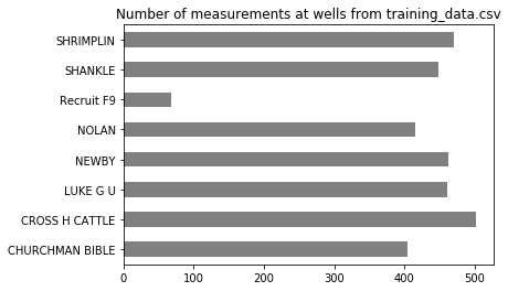
Figure 1: Number of facies measurements for each well in training_data.csv

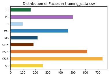
Figure 2: Distribuion of facies classes in training_data.csv

Attirbute	Facies	Depth	GR	ILD_log10	DeltaPHI	PHIND	PE	NM_M	RELPOS
Facies	1.000	0.340	-0.344	0.394	-0.234	-0.356	0.704	0.855	0.069
Depth		1.000	-0.064	0.178	-0.091	-0.074	0.278	0.297	0.001
GR			1.000	-0.156	0.190	0.248	-0.289	-0.281	-0.173
ILD_log10				1.000	-0.118	-0.523	0.385	0.519	0.088
DeltaPHI					1.000	-0.250	0.011	-0.174	0.037
PHIND						1.000	-0.573	-0.488	-0.035
PE							1.000	0.657	0.019
NM_M								1.000	0.037
RELPOS									1.000

Table 3: Correlation coefficients between scalar attributes

5.1 Feature examination: Resistivity

Resistivity describes the resistance of a material to the flow of electric current. It can be described by Eqn. 2 as follows:

$$R=\frac{r\cdot A}{L}=\frac{V\cdot A}{I\cdot L}$$ (2)

where R is resistivity of sample in unit of $\Omega m$, $r$ is resistance in unit of $\Omega$, $A$ is cross-section area of sample in un it of $m^{2}$ and $L$ is length of sample in unit of $m$.

A formation’s true resistivity $R_{t}$ is its resistivity when not contaminated by drilling fluids. It may contain formation water only or formation water and hydrocarbons. It is fundamental to use a valid $R_{t}$ for the presence of hydrocarbons when analyzing well log measurements. With the presence of drilling fluid’s invasion, resistivity of mud filtrate $R_{mf}$ can affect $R_{t}$ measurement. The measured resistivity can be either greater than, less than, or equal to $R_{t}$ and can distort deep resistivities. To get a valid $R_{t}$ value, corrections must be made to attenuate such distortions.

Fig. 3 shows drilling fluid corrected distribution of formation resisitivity $F$ in logrithmetic form $log_{10}F$ (attribute ILD_log10).

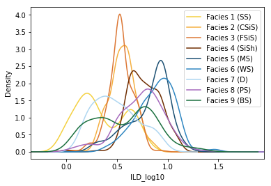
Figure 3: Distribution of $log_{10}F$ by facies

5.2 Feature examination: Neutron Density Porosity

Neutron logs are used to measure the hydrogen content in a formation. The emitted neutrons from a chemical source will collide with nuclei in the formation and thus lose energy. With enough collisions, a neutron will be absorbed by the formation and a $\gamma$-ray will be emitted. In neutron-hydrogen collisions, the average energy transfers to the hydrogen nucleus is about $\sim 50\%$ of the energy of the original neutron since the mass of a neutron is close to the mass of a hydrogen (proton). This indicates that materials with large hydrogen content will slow down neutrons.

In a porous formation, hydrogen contents tend to concentrate in the fluid-filled pores, formation’s porosity can thus by inferred by measuring neutron energy losses. Fig. 4 shows distribution of neutron density porosity $\phi$ in logrithmetic form $log_{10}\phi$ (attribute PHIND_log10).

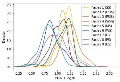
Figure 4: Distribution of $log_{10}\phi$ by facies

5.3 Relationship between Resistivity and Porosity

In the famous paper on classification of carbonate reservoir rocks and petrophysical considerations (Archie,, 1952), Archie proposed an empirical formula to calculate the water saturation ($S_{w}$) in a formation next to a borehole from well log parameters. This formula, known as Archie equation, is shown in Eqn. 3 below:

$$F=\frac{R_{0}}{R_{w}}=C\cdot\phi^{-m}$$ (3)

where $F$ is called formation resistivity, $R_{w}$ with unit $\Omega m$ is the resistivity of reservoir water, $R_{0}$ is the resistivity of reservoir rock saturated with reservoir water, and $R_{t}$ is the resistitivy of reservoir rock saturated with oil and water, $C$ is tortuousity constant, $m$ is cementation factor, which depends on rock formation. After taking the logrithmetic operation on both sides, Eqn. 3 can be re-written as:

$$log_{10}F=log_{10}C-m\cdot log_{10}\phi$$ (4)

Archie’s equation in the form of Eqn. 4, though empirical, suggests there exists a linear relationship between $log_{10}F$ and $log_{10}\phi$ which may vary for different rock types. This information, when provided, may further improve the accuracy of machine learning classification tasks.

For better display and without loss of generality, three facies (facies 1, 3, and 7) are chosen to generate $log_{10}F$ vs. $log_{10}\phi$ plot as shown in Fig. 5, with simple linear regression lines overlaid on top.

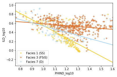
Figure 5: $log_{10}F$ vs. $log_{10}\phi$ scatter plot overlaid with linear regression lines

Fig. 5 suggests the ratio between logrithmetic resistivity $log_{10}F$ and logrithmetic neutron-density porosity $log_{10}\phi$ have good discrimination power for different facies. Fig.  5 also suggests the $log_{10}F$ vs. $log_{10}\phi$ discrimination power will not be the same for different facies pairs. For example, $log_{10}F$ vs. $log_{10}\phi$ can better discriminate facies 1 and facies 3 than facies 1 and facies 7.

6 Classifier Evaluation

Starting with benchmark, with additional feature augmentation using $\frac{log_{10}F}{log_{10}\phi}$, the final averaged F-1 score of 0.61 is achieved. This is a $\sim 5\%$ improvement over the benchmark F-1 score of 0.58 under the same settings.

A confusion matrix plot like Fig. 6a is used to give a more direct visual display of prediction accuracy for each facies class. In an ideal case using a perfect classifier, the confusion matrix should become an identity matrix $I_{n\times n}$, with all diagonal elements to be 1 and off-diagonal elements to be 0. The comparison of confusion matrix in Fig. 6a and in Fig. 6b clearly shows that confusion matrix from our solution is overall more focused around diagonal elements while reducing the values in off-diagonal elements, indicating an overal improvement in prediction accuracy.

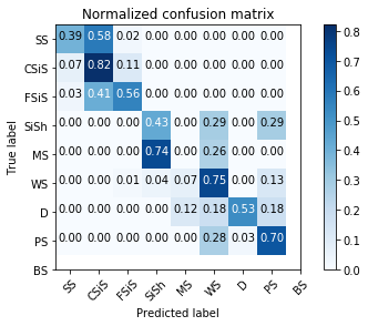
(a) from benchmark approach

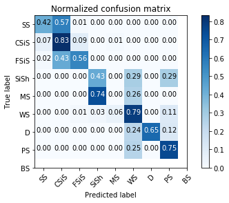
(b) from our approach

Figure 6: Comparison of normalized confusion matrix: benchmark approach vs. our approach

Fig. 7 shows a more obvious comparisons of true facies, predicted facies from benchmark approach and predicted facies from our approach. The 7 raw features are plotted on the left of the figure, while the true and predicted facies categories are plotted on the right, using the same depth information. Overall, our approach provides a better facies classification prediction than benchmark.

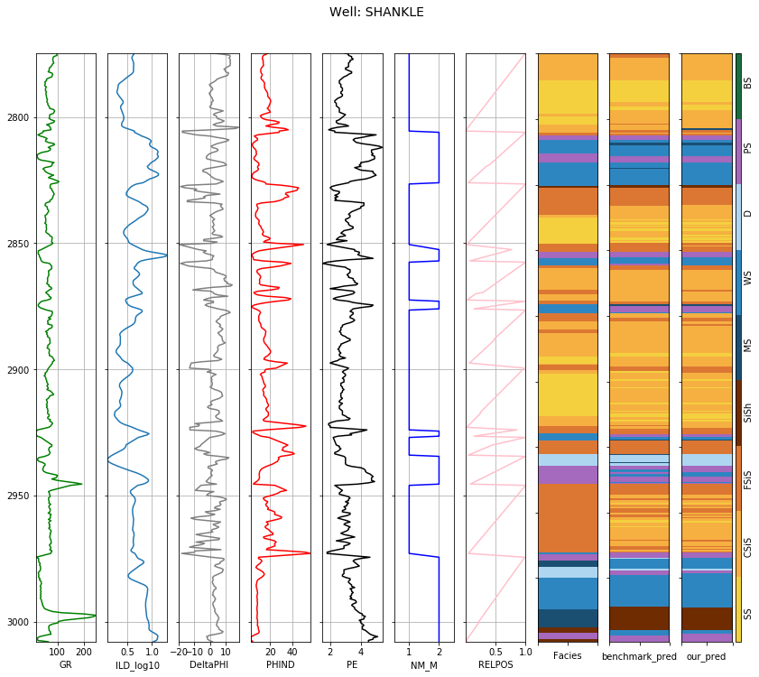
Figure 7: Wireline log measurements and comparison of facies classfication between true values, benchmark predictions and our predictions.

To verify the robustness of our approach, a few sanity checks are performed. To eliminate the possible bias introduced by the chosen random seed, we tested our approach using different random seeds and find the resulting improvement on F-1 score is robust and is consistently at $2\%\sim 7\%$ level. We also performed 7-fold cross-validation test by saving one of the 8 wells as blind well for test, and found the F-1 score is also improved at $\sim 5\%$ level consistently. As another cross check, with the same train/test/blind split and the same random state, we repeated the exactly identical SVM-based workflow as demonstrated in the SEG machine learning contest paper (Hall,, 2016) by adding new feature $\frac{log_{10}F}{log_{10}\phi}$ (i.e. ILD_log10/PHIND_log10), and the resulting F-1 score on blind evaluation dataset is increased from 0.43 to 0.44, which is $2.3\%$ improvement. These tests confirmed the uplift from our feature augmentation is robust against algorithm change, data sampling variation, and random seed initialization. Though better than benchmark with robust improvement, the model we obtained is still not perfect. As can be seen in Fig. 6 and Fig. 7, our model has trouble in making correct predictions for some facies, especifally those may blend into one another. A good example would be facies 4 (Marine siltstone and shale: SiSh) and facies 5 (Mudstone: MS). We expect further work on deep learning strategies for feature learning and inclusions of additional physical measurements can further improve the prediction accuracy.

7 Conclusion and Discussion

In this paper, we demonstrated feature augmentation incorporating domain knowledge can further improve the capability of machine learning. Motivated by Archie’s equation and with the inclusion of additional feature created from resistivity and porosity measurements, robust improvement in F-1 score is obtained and can be $\sim 5\%$ better over current existing best F-1 score. This example also shows there is ultimately no replacement for the insights human beings can put into feature engineering.

Currently, the dataset we use only contains limited number of physical attributes. To further improve in future rock facies classification tasks, additional types of well log measurements, including $V_{p}$, $V_{s}$, density etc., if provided, will probably further enhance machine learning’s capability in achieving better accuracy. For example, $V_{p}/V_{s}$ is directly related to the Poisson’s ratio (Gercek,, 2007), which measures the ratio of lateral strain to axial strain in a rock and can be served as another distinctive discriminator in facies classification.

For machine learning algorithms, the power of DNN seems to be limited by this relatively small dataset (Hall et al.,, 2017), leading to worse prediction accuracy when compared with XGBoost. Recently, a noval stochastic gradient descent method is proposed to overcome the requirement of large samples in traditional DNN (Wang et al.,, 2018). This would potentially improve the DNN-based F-1 score.

8 ACKNOWLEDGMENTS

The authors would like to thank the organizers of the SEG machine learning contest for making contest dataset and solution publicly available for further R&D.

References

- Hall, (2016) Hall, B., 2016, Facies classification using machine learning: The Leading Edge, 35, 906-909.
- Bestagini et al., (2017) Bestagini, P., V. Lipari, and S. Tubaro, 2017, A machine learning approach to facies classification using well logs: SEG Technical Program Expanded Abstracts, 2137-2142.
- Zhang et al., (2017) Zhang, L., and C. Zhan, 2017, Machine learning in rock facies classification - an application of XGBoost: International Geophysics Conference, Qingdao, China, 1371-1374.
- Hall et al., (2017) Hall, M. and B. Hall, 2017, Distribution collaborative prediction: Results of the machine learning contest: The Leading Edge, 36, 267-269.
- Sidahmed et al., (2017) Sidahmed, M., A. Roy, and A. Sayed, 2017, Streamline rock facies classification with deep learning cognitive process: SPE Annual Technical Conference and Exhibition.
- Archie, (1952) Archie, G.E., 1952, Classification of carbonate reservoir rocks and petrophysical considerations: AAPG, 36, 278-298.
- Pedregosa et al., (2011) Pedregosa, F. et al., 2011, Scikit-learn: Machine learning in python: Journal of Machine Learning Research, 12, 2825-2830.
- Dubois et al., (2007) Dubois, M., G. Bohling, and S. Chakrabarti, 2007, Comparison of four approaches to a rock facies classification problem: Computers and Geosciences, 33, 599-617.
- Hall et al., (2016) Hall, B., 2016, https://github.com/seg/2016-ml-contest
- Mosser et al., (2017) Mosser, P., and A. Briceno, 2017, https://github.com/seg/2016-ml-contest/tree/master/LA_Team
- Chen et al., (2016) Chen, T. and C. Guestrin, 2016, XGBoost: A scalable tree boosting system, arXiv: 1603.02754.
- Friedman, (2001) Friedman, J. H., 2001, Greedy function approximation: A gradient boosting machine: The Annuals of Statistics, 29, 1189-1232.
- Friedman, (2008) Friedman, J. H., and B. E. Popescu, 2008, Predictive learning via rule ensembles: The Annuals of Applied Statistics, 2, 916-954.
- Chevitarese et al., (2018) Chevitarese, D.S., D. Szwarcman, R.M. Gama e Silva and E. Vital Brazil, 2018, Deep learning applied to seismic facies classification: a methodology for training, Saint Petersburg 2018, Russia.
- Mikhailiuk et al., (2018) Mikhailiuk, A., and A. Faul, 2018, Deep learning applied to seismic data interpolation: 80th EAGE Conference and Exihibition.
- Gercek, (2007) Gercek, H., 2007, Poisson’s ratio values for rocks: International Journal of Rock Mechanics and Mining Sciences, 44, 1-13.
- Wang et al., (2018) Wang, G., G.B. Giannakis and J. Chen, 2018, Learning ReLU networks on linearly separable data: algorithm, optimality, and generalization, arXiv: 1808.04685.