Generalizations of TASEP in discrete and continuous inhomogeneous space

Abstract

We investigate a rich new class of exactly solvable particle systems generalizing the Totally Asymmetric Simple Exclusion Process (TASEP). Our particle systems can be thought of as new exactly solvable examples of tandem queues, directed first- or last-passage percolation models, or Robinson-Schensted-Knuth type systems with random input. One of the novel features of the particle systems is the presence of spatial inhomogeneity which can lead to the formation of traffic jams.

For systems with special step-like initial data, we find explicit limit shapes, describe hydrodynamic evolution, and obtain asymptotic fluctuation results which put the systems into the Kardar-Parisi-Zhang universality class. At a critical scaling around a traffic jam in the continuous space TASEP, we observe deformations of the Tracy-Widom distribution and the extended Airy kernel, revealing the finer structure of this novel type of phase transitions.

A homogeneous version of a discrete space system we consider is a one-parameter deformation of the geometric last-passage percolation, and we obtain extensions of the limit shape parabola and the corresponding asymptotic fluctuation results.

The exact solvability and asymptotic behavior results are powered by a new nontrivial connection to Schur measures and processes.

1 Introduction

1.1 Discrete time TASEP

The paper’s main goal is two-fold:

1. We introduce new stochastic particle systems in discrete and continuous inhomogeneous space generalizing the well-known Totally Asymmetric Simple Exclusion Process (TASEP), and express their observables (with arbitrary inhomogeneity) through Schur measures, a widely used tool for getting asymptotic fluctuations in a variety of stochastic systems in one and two spatial dimensions;

2. In a continuous space system which we call the continuous space TASEP, we study the effect of spatial inhomogeneity on the fluctuation distribution around the traffic jam, and obtain a phase transition of a novel type.

We begin by recalling the original TASEP, and in the next subsection define its extension which gives rise to new exactly solvable systems in inhomogeneous space.

The TASEP is one of the most studied nonequilibrium particle systems [Spi70], [Kru91], [Joh00], with applications ranging from protein synthesis [MGP68], [ZDS11] to traffic modeling [Hel01]. TASEP in discrete time is a Markov process on particle configurations in $\mathbb{Z}$ (with at most one particle per site) which evolves as follows. During each discrete time step $T-1\to T$, every particle flips an independent $p$-coin to decide whether it wants to jump one step to the right. Suppose the coin flip for some particle indicates a jump attempt. If the site to the right is vacant, the particle makes the jump, otherwise it remains in the same position. See Figure 1 for an illustration.

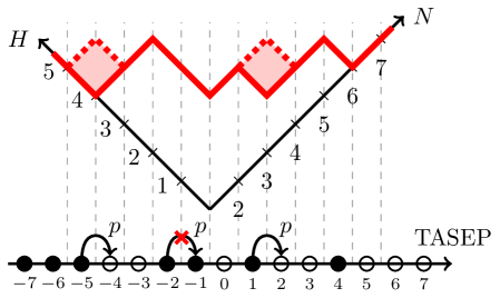
Figure 1: Discrete time TASEP with parallel update and its interpretation as a geometric corner growth. In this time step three particles make a jump attempt but one of them is blocked.

Start the TASEP from the step initial configuration under which the particles occupy every site of $\mathbb{Z}_{<0}$, and there are no particles in $\mathbb{Z}_{\geq 0}$. Let $h(T,x)$ be the random height function of the TASEP, that is, the number of particles to the right of $x\in\mathbb{Z}$ at time $T$. At the level of Law of Large Numbers, the height function grows linearly with time, and its macroscopic shape evolves according to the hydrodynamic equation [Lig05], [Spo91], [Lig99]. The first Central Limit Theorem type result on fluctuations of the height functions was obtained about two decades ago:

Theorem 1.1 ([Joh00]).

There exist functions $c_{1}(\kappa),c_{2}(\kappa)$ such that

$$\lim_{T\to\infty}\mathop{\mathrm{Prob}}\left(\frac{h(T,\lfloor\kappa T\rfloor)-c_{1}(\kappa)T}{c_{2}(\kappa)T^{1/3}}>-r\right)=F_{GUE}(r),\qquad r\in\mathbb{R},$$

where $F_{GUE}$ is the GUE Tracy-Widom distribution [TW94].

In particular, TASEP fluctuations live on the on $T^{1/3}$ scale, in contrast with the $T^{1/2}$ scale observed in probabilistic systems based on sums of independent random variables. This result puts TASEP into the Kardar-Parisi-Zhang (KPZ) universality class [FS11], [Cor12], [HHT15], [QS15], [Cor16].

There has been much development in further understanding the asymptotic behavior of TASEP and related models, including effects of different initial conditions and different particle speeds [ITW01], [GTW02], [PS02], [IS05], [BFPS07], [BFS09], [MQR17]. Much of this work relies on exact solvability of TASEP which is powered by the algebraic structure of Schur measures and processes [Oko01], [OR03]. An extension of Theorem 1.1 to ASEP (in which particles can jump in both directions) was proved a decade ago in the pioneering work of Tracy and Widom [TW09]. This has brought new exciting tools of Macdonald polynomials, Bethe Ansatz, and Yang-Baxter equation into the study of stochastic interacting particle systems [BC14], [BP16].

One important aspect of TASEP asymptotics that has been quite hard to understand deals with running TASEP in inhomogeneous space. By this we mean that each particle’s jumping probability $p=p_{x}$ depends on the particle’s current location $x$. For the inhomogeneous space TASEP the exact solvability (connections to Schur measures and processes or Bethe Ansatz) seems to break down. Recent progress has been made in a particular case of the slow bond TASEP. Namely, if $p_{x}=1$ everywhere except $p_{0}=1-\varepsilon$, then for any $\varepsilon>0$ the macroscopic speed of the TASEP at $0$ decreases [BSS14] (see also the previous works [JL92], [Sep01], [CLST13]). A Central Limit Theorem for $T^{1/2}$ Gaussian fluctuations in the slow bond TASEP was established in [BSS17].

1.2 Doubly geometric corner growth in discrete space

Let us reinterpret the TASEP with step initial configuration described above as a geometric corner growth model. The corner growth is a discrete time Markov process on the space of weakly decreasing height functions (or interfaces) $H\colon\mathbb{Z}_{\geq 1}\to\mathbb{Z}_{\geq 0}$ such that $H(1)=+\infty$ and $H(N)=0$ for large enough $N$. Initially, we have $H_{0}(N)=0$ for all $N\geq 2$, and at each discrete time step we independently add a $1\times 1$ box to every inner corner of the interface with probability $p$. Adding a box corresponds to a jump of one particle in the TASEP. See Figure 1, where the interface is rotated by $45^{\circ}$ to match with the particle system.

We are now in a position to describe an inhomogeneous extension of TASEP in this corner growth language, after specifying the parameter families.

Definition 1.2 (Discrete parameters).

The discrete systems we consider depend on the following parameters:

$$\begin{array}[]{ll}a_{i}\in(0,+\infty),&\quad i=1,2,\ldots;\\ \beta_{t}\in(0,+\infty),&\quad t=1,2,\ldots;\\ \nu_{j}\in\bigl{[}-\inf_{t\geq 1,i\geq 1}(\beta_{t}a_{i}),1\bigl{)},&\quad j=2,3,\ldots.\end{array}$$ (1.1)

The parameters in each of the families are assumed to be uniformly bounded away from the open boundaries of the corresponding intervals.

The doubly geometric inhomogeneous corner growth model (DGCG, for short) is, by definition, a discrete time Markov chain $H_{T}(N)$ on the space of height functions, where $N$ is the spatial variable and $T$ means discrete time.

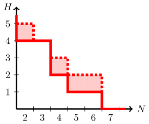
Figure 2: A possible step in DGCG. The inner corners before the step are at locations $2,4,5$, and $7$.

The random growth proceeds as follows. Let $2=N_{1}<\ldots<N_{k}$ be all inner corners of $H_{T}$, i.e., all locations at which $H_{T}(N_{i}-1)>H_{T}(N_{i})$. During the time step $T\to T+1$, at every inner corner $N_{i}$ we independently add a $1\times 1$ box (i.e., increase the interface at $N_{i}$ by one) with probability

$$\mathop{\mathrm{Prob}}\left(\textnormal{add a box at inner corner $N_{i}$ at step $T\to T+1$}\right)=\frac{\beta_{t+1}a_{N_{i}-1}}{1+\beta_{t+1}a_{N_{i}-1}}.$$ (1.2)

If a box at $N_{i}$ is added, we also instantaneously add an independent random number $\leq N_{i+1}-N_{i}-1$ (with $N_{k+1}=+\infty$, by agreement) of boxes to the right of it according to the truncated inhomogeneous geometric distribution

$$\mathop{\mathrm{Prob}}\left(\textnormal{add $0\leq m\leq N_{i+1}-N_{i}-1$ more boxes}\right)\\ =\begin{cases}\mathsf{p}(0)\mathsf{p}(1)\ldots\mathsf{p}(m-1)\bigl{(}1-\mathsf{p}(m)\bigr{)},&0\leq m<N_{i+1}-N_{i}-1;\\ \mathsf{p}(0)\mathsf{p}(1)\ldots\mathsf{p}(N_{i+1}-N_{i}-2),&m=N_{i+1}-N_{i}-1,\\ \end{cases}$$ (1.3)

where

$$\mathsf{p}(r)=p_{T+1,N_{i}}(r):=\frac{\nu_{r+N_{i}}+\beta_{t+1}a_{r+N_{i}}}{1+\beta_{t+1}a_{r+N_{i}}}$$ (1.4)

(note that this quantity is nonnegative, as it should be). See Figure 2 for an illustration.

In the simpler homogeneous case $a_{i}\equiv 1$, $\beta_{t}\equiv\beta$, $\nu_{j}\equiv\nu$ (note that setting $a_{i}$ to the particular constant $1$ does not restrict the generality of the homogeneous model), the random growth $H_{T}(N)$ uses two independent identically distributed families of geometric random variables (hence the name “doubly geometric corner growth”):

1. A new $1\times 1$ box is added after a geometric waiting time with probability of success $\frac{\beta}{1+\beta}$.

2. If a box is added, we also instantaneously add an independent random number of $1\times 1$ boxes to the right of the added box according to the truncated geometric distribution

   $$\mathop{\mathrm{Prob}}(\textnormal{add $0\leq m\leq M$ more boxes})=\begin{cases}\Bigl{(}\frac{\nu+\beta}{1+\beta}\Bigr{)}^{m}\frac{1-\nu}{1+\beta},&0\leq m<M;\\[12.0pt] \Bigl{(}\frac{\nu+\beta}{1+\beta}\Bigr{)}^{M},&m=M,\end{cases}$$ (1.5)

   where $M$ is the maximal number of boxes which can be added without overhanging.

Remark 1.3.

When we formally set $\nu=-\beta$ and $p=\frac{\beta}{1+\beta}$, the homogeneous DGCG model becomes the usual TASEP (in its geometric corner growth formulation). Indeed, for $\nu=-\beta$ no extra boxes are instantaneously added to the randomly growing interface. In Section 6 we discuss the relation between the limit shape of the usual geometric corner growth and the homogeneous DGCG model.

The homogeneous DGCG was suggested in [DPPP12], [Pov13] and further studied (on a ring) in [DPP15]. Similar tandem queuing and first-passage percolation models also appeared earlier in [Woe05], [Mar09].

1.3 Continuous space TASEP

Let us now describe our second and main model, the continuous space TASEP. It is a continuous time Markov process on the space of finite particle configurations in $\mathbb{R}_{>0}$. The particles are ordered, and the process preserves the ordering. More than one particle per site is allowed, and one should think that particles at the same site form a vertical stack (consisting of $\geq 1$ particles). It is convenient to think that there is an infinite stack of particles at location $0$.

The process depends on a speed function $\xi(y)$, $y\in\mathbb{R}_{\geq 0}$, which is assumed positive, piecewise continuous, and bounded away from $0$ and $+\infty$. We also need a scale parameter $L>0$ which will later go to infinity. The process evolves as follows:

Definition 1.4 (Evolution of the continuous space TASEP).

New particles leave the infinite stack at $0$ at rate $\xi(0)$. If there are particles in a stack located at $x\in\mathbb{R}_{>0}$, then one particle may (independently) decide to leave this stack at rate $\xi(x)$. Almost surely at each moment in time only one particle can start moving. Finally, the moving particle instantaneously jumps to the right by a random distance $\min(Y,x^{(r)}-x)$, where $Y$ is an independent exponential random variable with mean $1/L$, and $x^{(r)}$ is the coordinate of the nearest stack to the right of the one at $x$ ($x^{(r)}=+\infty$ if there are no stacks to the right of $x$). In other words, if the desired moving distance is too large, then the moving particle joins the stack immediately to the right of its old location.

See Figure 3 for an illustration.

Figure 3: A possible jump in the continuous space TASEP.

The continuous space TASEP arises from the DGCG in a certain Poisson type limit transition which preserves exact solvability. We study asymptotic behavior of the continuous space TASEP in an arbitrary landscape described by the function $\xi(\cdot)$. We obtain the limit shape and investigate fluctuations and phase transitions at points of discontinuous decrease in $\xi$. These points can be interpreted as traffic accidents, road work, or drastic changes in the landscape, and may lead to traffic jams. By a traffic jam we mean the presence of a large number of particles in a small interval, which corresponds to a discontinuity of the macroscopic height function.

Remark 1.5.

It is possible to add obstacles of another type to the continuous space TASEP. These are fixed sites $b\in\mathbb{R}_{>0}$ (interpreted as traffic lights or roadblocks) which with some positive probability capture particles flying over them (precise definition in Section 2.3). Roadblocks may create shocks of Baik-Ben Arous-Péché type. The corresponding asymptotic results are given in Section 4.

1.4 Results

Let $H_{T}(N)$ be the height function (= interface) of DGCG with the initial condition $H_{0}(N)=0$ for $N\geq 2$. In the continuous space TASEP, let $\mathcal{H}(t,\chi)$ count the number of particles to the right of the location $\chi$ at time $t$ (when initially the line $\mathbb{R}_{>0}$ has no particles). The first main result of the paper connect both families of random variables $\left\{H_{T}(N)\right\}_{T}$ and $\left\{\mathcal{H}(t,\chi)\right\}_{t}$ (for fixed $N$ and $\chi$, respectively) to determinantal processes. In particular, the joint distribution of $\left\{H_{T_{j}}(N+1)\right\}$ coincides with the joint distribution of the leftmost points in a certain Schur process depending on the parameters $a_{1},\ldots,a_{N}$, $\left\{\beta_{t}\right\}$, and $\nu_{2},\ldots,\nu_{N}$. The determinantal structure of the continuous space TASEP’s height function $\left\{\mathcal{H}(t,\chi)\right\}_{t}$ is obtained as a limit from the DGCG case. See Sections 3.2 and 3.3 for detailed formulations of structural results.

Our second group of results concern asymptotic analysis. Using the determinantal structure, we investigate the asymptotic behavior of the continuous space TASEP, that is, study $\mathcal{H}(\theta L,\chi)$ as $L\to\infty$ and the speed function $\xi(\cdot)$ is fixed (there is no need to scale the continuous space). Our asymptotic results are the following:

1. (Law of Large Numbers; Theorem 4.5) We show that there exists a deterministic limit (in probability) of the rescaled height function $L^{-1}\mathcal{H}(\theta L,\chi)$ as $L\to+\infty$. The limit shapes is a Legendre dual of an explicit function involving an integral over the inhomogeneous space.

2. (Hydrodynamic equations; Appendix B) We present informal derivations of hydrodynamic partial differential equations for the limiting densities in DGCG and the continuous space TASEP. This is done by constructing families of local translation invariant stationary distributions of arbitrary density, and computing the flux (also called current) of particles.

3. (Central Limit type Theorem; Theorem 4.6) We show that generically the fluctuations of the height function around the limit shape are of order $L^{1/3}$ and are governed by the GUE Tracy-Widom distribution as in Theorem 1.1. We also consider the corresponding fluctuations at a single location and different times, leading to the Airy₂ process. In the presence of shocks caused by roadblocks we observe a phase transition of Baik-Ben Arous-Péché type.

4. (Fluctuations in traffic jams; Theorem 4.7) The most striking feature of our asymptotic results is a phase transition of a new type in the continuous space TASEP. Namely, there is a transition in fluctuation distribution as one approaches a point of discontinuous decrease in the speed function $\xi(\cdot)$ from the right. There is a critical distance from the jump discontinuity of $\xi(\cdot)$ at which the fluctuations are governed by a deformation of the GUE Tracy-Widom distribution. This deformation can in principle be also obtained in a limit of an inhomogeneous last-passage percolation, or in a multiparameter Wishart-like random matrix model. Both models were considered in [BP08], and our kernel for the deformed GUE Tracy-Widom distribution is a particular case of formula (6) in that paper.

We leave a detailed investigation of the DGCG model (including phase transitions in fluctuations) for a future work. Here we only consider the homogeneous DGCG which depends on two parameters $\beta>0$ and $\nu\in[-\beta,1)$ and is a one-parameter extension of the standard corner growth model. We show (Section 6) that the limit shape in the homogeneous DGCG is a one-parameter deformation of the corner growth’s limit shape parabola, and obtain the corresponding GUE Tracy-Widom fluctuations.

1.5 Methods

Since the seminal works [BDJ99], [Joh00], [BOO00], [Oko01], [OR03] about two decades ago, Schur measures and processes proved to be a very successful tool in the asymptotic analysis of a large class of interacting particle systems and models of statistical mechanics. These methods of Integrable Probability also serve as our main analytic tool. However, the connection between the models we consider and Schur processes is not that apparent. We consider establishing and utilizing this connection an important part of the paper. From this point of view, DGCG and continuous TASEP extend the field of classical models solved by means of Schur functions.

Curiously, it became possible to find this connection to Schur processes only due to recent developments in the study of stochastic higher spin six vertex models. Namely, the continuous space TASEP is a $q\searrow 0$ degeneration of the inhomogeneous exponential jump model studied in [BP18a]. The methods used in that paper involved computing $q$-moments of the height function of the model, and break down for $q=0$ (see Section 2.4 below for more detail). Here we apply a different approach based on a nontrivial coupling [OP17] between the stochastic higher spin six vertex model and $q$-Whittaker measures and processes. This coupling survives passing to the $q\searrow 0$ limit and produces a coupling between DGCG and Schur processes, which circumvents the issue of not having observables of $q$-moment type for $q=0$. Moreover, at $q=0$ the $q$-Whittaker processes turn into the Schur ones which possess determinantal structure [Oko01], [OR03].

The passage from DGCG to the continuous space TASEP preserves the determinantal structure coming from the Schur measures. The determinantal process associated with the continuous space TASEP lives on infinite particle configurations and depends on the arbitrary speed function $\xi(\cdot)$. In particular cases this limit transition has appeared in [BO07], [BD11], [BO17]. In full generality this limit of Schur measures and processes seems new.

To obtain our asymptotic results, we perform analysis of the correlation kernel (written in a double contour integral form) by the steepest descent method. Because of the presence of inhomogeneity parameters in the kernel, the steepest descent analysis requires several difficult technical estimates.

We also note that using the determinantal methods of Schur measures and processes we are able to analyze the asymptotic behavior of joint distributions of the height function at different times (of either DGCG or the continuous space TASEP) at a single location. It is interesting that the Schur structure we employ does not cover joint distributions at several space locations (see Section 2.4 for more discussion). A companion paper [Pet19] deals with a simpler model in inhomogeneous space in which an analysis of certain joint distributions across space and time is possible.

1.6 Equivalent formulations

Both the DGCG and the continuous space TASEP possess a number of equivalent formulations and interpretations most of which mimic equivalences known for the usual TASEP.

The doubly geometric corner growth model has the following interpretations:

1. A corner growth model, the original definition in Section 1.2;

2. A generalization of the classical TASEP from Section 1.1 in which the jumping distance of each particle is the product of independent Bernoulli and the geometric random variables:

   $$\mathop{\mathrm{Prob}}(j)=\frac{\mathbf{1}_{j=0}}{1+\beta}+\frac{\beta\,\mathbf{1}_{j\geq 1}}{1+\beta}\left(\frac{\nu+\beta}{1+\beta}\right)^{j-1}\frac{1-\nu}{1+\beta},\qquad j\in\mathbb{Z}_{\geq 0}.$$ (1.6)

   Jumping over the particle to the right is forbidden. See Figure 4 for an illustration, and Section A.1 for more detail. We call (1.6) the geometric-Bernoulli distribution (or gB distribution, for short).

   

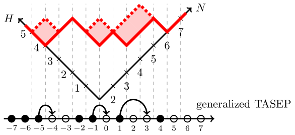
   Figure 4: DGCG model and its matching to a generalization of TASEP which we call the gB-TASEP.

3. Via the exclusion/zero range duality (essentially, by looking at the growing DGCG interface in the $(H,N)$ coordinates) the DGCG can be interpreted as a zero range process with the gB hopping distribution.

4. A directed last-passage percolation model with a random environment type modification (Section A.2).

5. A directed first-passage percolation model on a strict-weak lattice with independent gB distributed weights (Section A.3). This interpretation is closely related to applying the column Robinson-Schensted-Knuth (RSK) correspondence to a random matrix with independent gB distributed entries. Limit shapes for this (homogeneous) model were considered previously in [Mar09].

6. A free fermion type degeneration of the stochastic higher spin six vertex model studied in, e.g., [Bor17], [CP16], [BP18].

7. Via a coupling of [OP17], certain observables of the (free fermion degenerate) stochastic higher spin six vertex model are mapped to those in a TASEP with time-mixed geometric and Bernoulli steps. The latter is directly linked to Schur processes providing a crucial ingredient for exact solvability of the DGCG.

The last two interpretations are explained in Section 2, and are crucially employed in the proof of the determinantal structure of DGCG and continuous space TASEP in Section 3.

In the limit to the continuous space TASEP the first-passage percolation model coming out of DGCG turns into a semi-discrete directed first-passage percolation, with a modification that each point of a Poisson process has an additional independent exponential weight. See Section A.4.

Moreover, the continuous space TASEP has a natural formulation as a continuous time tandem queuing system. The jobs (= particles) enter the system according to a Poisson clock at $0$. Each point of the real line is a server with exponential service times (and the rate depends on the server’s coordinate). The job processed at one server is sent to the right (according to an exponential random distance with mean $1/L$) and either joins the queue at the nearest server on the right, or forms a new queue.

1.7 Related work on spatially inhomogeneous systems

The study of interacting particle systems in inhomogeneous space started with numerical and hydrodynamic analysis. Numerical simulations were mainly motivated by applications to traffic modeling [KF96], [Ben+99], [Kru00], [DZS08], [Hel01].

The hydrodynamic treatment of interacting particle systems is the main tool of their asymptotic analysis [Lig05], [Lig76], [And82], [AK84], [Spo91], [Lig99] in the absence of exact formulas. This technique allows to prove the law of large numbers and write down a macroscopic PDE for the limit shape of the height function. Hydrodynamic methods have been successfully applied to spatially inhomogeneous systems including TASEP in, e.g., [Lan96], [Sep99], [RT08], [GKS10], [Cal15].

Limit shapes of directed last-passage percolation in random inhomogeneous environment have been studied in [SK99] and more recently in [Emr16], [CG18]. Other spatially inhomogeneous systems were considered in, e.g., [BNKR94], [TTCB10], [Bla11], [Bla12], with focus on condensation/clustering effects and understanding of phase diagrams.

A stochastic partial differential equation limit of the spatially inhomogeneous ASEP was obtained recently in [CT18]. This limit regime to an SPDE differs from the one we consider since one needs to scale down the ASEP asymmetry, while we work in a totally asymmetric setting from the beginning.

Rigorously proving asymptotic results on fluctuations in interacting particle systems in the KPZ universality class typically require exact formulas. A first example of such a result is Theorem 1.1 of [Joh00] which essentially utilizes Schur measures. In the presence of spatial inhomogeneity, however, integrable structures in systems like TASEP break down. In fact, the understanding of asymptotic fluctuations remains a challenge for most spatially inhomogeneous systems in the KPZ class. An exception is the Gaussian fluctuation behavior in the slow bond TASEP established recently in [BSS17]. In contrast, inserting particle-dependent inhomogeneity parameters (i.e., when particles have different speeds) preserves most of the structure which allows to get asymptotic fluctuations, e.g., see [Bai06], [BFS09], [Dui13], [Bar15].

In principle, the $(\textnormal{time})^{1/3}$ scale of fluctuations in certain spatially inhomogeneous zero range processes may be established as in [BKS12], but this does not give access to fluctuation distributions. The previous work [BP18a] is a first example of rigorous fluctuation asymptotics (to the point of establishing Tracy-Widom fluctuation distributions) in a spatially inhomogeneous TASEP-like particle system (which is a $q$-deformation of our continuous space TASEP). The present work improves on the results of [BP18a] by treating joint fluctuations in the $q=0$ system and looking at fluctuations close to traffic jams. Overall, in this paper we explore a whole new family of natural exactly solvable systems with spatial inhomogeneity.

1.8 Outline

The paper is organized as follows. In Section 2 we describe how the DGCG model is related to a (free fermion) stochastic higher spin six vertex model, and get the continuous space TASEP as a Poisson-type limit of DGCG. We also recall the (degeneration of) the result of [OP17] linking the stochastic vertex model to a TASEP with mixed geometric and Bernoulli steps. In Section 3 we show how the latter connection leads to a determinantal structure in both the DGCG and continuous space TASEP models. In Section 4 we formulate the asymptotic results about the continuous space TASEP and the homogeneous DGCG, and prove them in Section 5. In Section 6 we discuss the homogeneous version of the DGCG model, obtain its limit shape and fluctuations, and show that they present a one-parameter extension of the celebrated geometric corner growth model.

In Appendix A we discuss in detail a number of equivalent combinatorial formulations of the DGCG and the continuous space TASEP. Appendix B presents informal derivations of hydrodynamic partial differential equations. Appendix C contains the definitions of various fluctuation kernels appearing in the paper.

Notation.

Throughout the paper $C,C_{i},c,c_{j}$ stand for positive constants which are independent of the main asymptotic parameter $L\to+\infty$. The values of the constants might change from line to line.

2 Stochastic vertex models and particle systems

Here we explain how the DGCG and continuous space TASEP defined in Sections 1.2 and 1.3 are related to a certain stochastic vertex model. Joint distributions of the height function in the latter model are coupled to a TASEP with time-mixed geometric and Bernoulli steps via results of [OP17] which we also recall.

2.1 Schur vertex model

We begin by describing a stochastic vertex model whose height function coincides with the DGCG interface $H_{N}(T)$. Both models depend on the parameters $a_{i},\nu_{j},\beta_{t}$ from Definition 1.2.

First we recall a $q$-dependent inhomogeneous stochastic higher spin six vertex introduced in [BP18]. We follow the notation of [OP17] with the agreement that the parameters $u_{i}$ in the latter paper are expressed through our parameters as $u_{t}\equiv-\beta_{t}>0$, $t=1,2,\ldots$. The stochastic higher spin six vertex model is a probability distribution on the set of infinite oriented up-right paths drawn in $(N,T)\in\mathbb{Z}_{\geq 2}\times\mathbb{Z}_{\geq 1}$, with all paths starting from a left-to-right arrow entering at some of the points $\{(2,T)\colon T\in\mathbb{Z}_{\geq 1}\}$ on the left boundary. No paths enter through the bottom boundary. Paths cannot share horizontal pieces, but common vertices and vertical pieces are allowed. The probability distribution on this set of paths is constructed in a Markovian way. First, we flip independent coins with probability of success $a_{1}\beta_{T}/(1+a_{1}\beta_{T})$, $t\in\mathbb{Z}_{\geq 1}$, and for each success start a path at the point $(2,T)$ on the left boundary.

Figure 5: Sampling a path configuration inductively.

Then, assume that we have already defined the configuration inside the triangle $\{(N,T)\colon N+T\leq n\}$, where $n\geq 2$. For each vertex $(N,T)$ with $N+T=n$, we know the number of incoming arrows (from below and from the left) into this vertex. Sample, independently for each such vertex, the number of outgoing arrows according to the stochastic vertex weights $\mathsf{L}^{(q)}_{a_{N},\nu_{N},\beta_{T}}$ given in Definition 2.1 below. In this way the path configuration is now defined inside the larger triangle $\{(N,T)\colon N+T\leq n+1\}$, and we can continue inductively. See Figure 5 for an illustration.

Definition 2.1.

The ($q$-dependent) vertex weights is a collection $\mathsf{L}^{(q)}_{a,\nu,\beta}(i_{1},j_{1};i_{2},j_{2})$, $i_{1},i_{2}\in\mathbb{Z}_{\geq 0}$, $j_{1},j_{2}\in\{0,1\}$, where $i_{1}$ and $j_{1}$ are the numbers of arrows entering the vertex, respectively, from below and from the left, and $i_{2}$ and $j_{2}$ are the numbers of arrows leaving the vertex, respectively, upwards and to the right. The concrete expressions for $\mathsf{L}^{(q)}_{a,\nu,\beta}$ are given in the following table:

$$\mathsf{L}^{(q)}_{a,\nu,\beta}$$ —

Here $g\in\mathbb{Z}_{\geq 0}$ is arbitrary. Note that the weight automatically vanishes at the forbidden configuration $(0,0;-1,1)$.

We impose the arrow preservation property: $\mathsf{L}^{(q)}_{a,\nu,\beta}(i_{1},j_{1};i_{2},j_{2})$ vanishes unless $i_{1}+j_{1}=i_{2}+j_{2}$ (i.e., the number of outgoing arrows is the same as the number of incoming ones). Moreover, the weights are stochastic:

$$\sum_{i_{2},j_{2}\in\mathbb{Z}_{\geq 0}\colon i_{2}+j_{2}=i_{1}+j_{1}}\mathsf{L}^{(q)}_{a,\nu,\beta}(i_{1},j_{1};i_{2},j_{2})=1,\qquad\mathsf{L}^{(q)}_{a,\nu,\beta}(i_{1},j_{1};i_{2},j_{2})\geq 0.$$ (2.1)

The nonnegativity of the weights holds if $q\in[0,1)$, $a,\beta\in(0,+\infty)$, and $\nu\geq-a\beta$. We can thus interpret $\mathsf{L}^{(q)}_{a,\nu,\beta}(i_{1},j_{1};i_{2},j_{2})$ as a (conditional) probability that there are $i_{2}$ and $j_{2}$ arrows leaving the vertex given that there are $i_{1}$ and $j_{1}$ arrows entering the vertex.

The weights $\mathsf{L}^{(q)}_{a,\nu,\beta}$ remain stochastic when setting $q=0$. The new vertex weights depend on whether $i_{1}$ is zero or not, and are given in Figure 6. We call the corresponding stochastic higher spin six vertex model the Schur vertex model due to its connections with Schur measures which we explore later.

$\mathsf{L}^{(q=0)}_{a,\nu,\beta}$	$1$	$\dfrac{\nu+a\beta}{1+a\beta}$	$\dfrac{1-\nu}{1+a\beta}$ —
$\mathsf{L}^{(q=0)}_{a,\nu,\beta}$	$\dfrac{1}{1+a\beta}$	$\dfrac{a\beta}{1+a\beta}$	$\dfrac{a\beta}{1+a\beta}$	$\dfrac{1}{1+a\beta}$ —

Figure 6: The vertex weights for $q=0$. Everywhere in the second row we have $g\geq 1$.

Figure 7: A step $T\to T+1$ in the Schur vertex model viewed as a parallel update. The path at $2$ decides to travel by $2$. The path at $5$ starts traveling, but when it reaches $6$ it has to stop. The path at $6$ decides not to travel.

One crucial observation regarding the $q=0$ weights in Figure 6 is that $\mathsf{L}^{(q=0)}_{a,\nu,\beta}(i_{1},j_{1};i_{2},j_{2})$ depends on $j_{1}$ only if $i_{1}=0$. That is, the evolution $T\to T+1$ in the Schur vertex can be regarded as a parallel update (for this reason one can say that setting $q=0$ means a “free fermion” degeneration). In particular, each nonempty cluster of paths at each horizontal coordinate $N$ independently decides (with probability $a_{N}\beta_{T+1}/(1+a_{N}\beta_{T+1})$) to emit one path which travels to the right. This traveling path then makes a random number of steps to the right, at each step deciding to continue or to stop with probabilities corresponding to the vertices $(0,1;0,1)$ or $(0,1;1,0)$, respectively. If the path reaches the neighboring cluster of paths on the right, then it has to stop. See Figure 7 for an illustration. This establishes a correspondence between the Schur vertex model and the DGCG model from Section 1.2:

Proposition 2.2.

The height function of the $q=0$ vertex model

$$H_{T}(N)=\#\{\textnormal{paths which are $\geq N$ at vertical coordinate $T$}\}$$

is the same as $H_{T}(N)$ in the DGCG model.

2.2 TASEP with mixed geometric and Bernoulli steps

This subsection is essentially a citation (and a $q=0$ degeneration) of [OP17] mapping the Schur vertex model to a TASEP with mixed steps. We continue to work with the parameters $a_{i},\beta_{t},\nu_{j}$ as in Definition 1.2, but in addition require that $\nu_{j}\geq 0$. In the mixed TASEP, the inhomogeneity is put onto particles, not space: each particle $Y_{i}$ is assigned the parameter $a_{i}$.

Definition 2.3.

The geometric step with parameter $\alpha>0$ such that $a_{i}\alpha<1$ for all $i$ applied to a configuration $\vec{Y}=(Y_{1}>Y_{2}>\ldots)$ in $\mathbb{Z}$ (with at most particle per site and densely packed at $-\infty$) is defined as follows. Each particle $Y_{j}$ with an empty site to the right (almost surely there are finitely many such particles at any finite time) samples an independent geometric random variable $\mathsf{g}_{j}$ with distribution

$$\mathop{\mathrm{Prob}}(\mathsf{g}_{j}=m)=(a_{j}\alpha)^{m}(1-a_{j}\alpha),\qquad m\in\mathbb{Z}_{\geq 0},$$

and jumps by $\min(\mathsf{g}_{j},Y_{j-1}-Y_{j}-1)$ steps to the right (with $Y_{0}=+\infty$ by agreement). See Figure 4 in the Introduction for an illustration of a possible jump (though note that the jump’s distribution differs from the one in the figure). When $\alpha=0$, the geometric step does not change the configuration.

Definition 2.4.

Under the Bernoulli step with parameter $\beta>0$, the configuration $\vec{Y}$ is randomly updated as follows. First, each particle $Y_{j}$ tosses an independent coin with probability of success $a_{j}\beta/(1+a_{j}\beta)$. Then, sequentially for $j=1,2,\ldots$, the particle $Y_{j}$ jumps to the right by one if its coin is a success and the destination is unoccupied. If the coin is a failure or the destination is occupied, the particle $Y_{j}$ stays put. (The first particle $Y_{1}$ moves with probability $a_{1}\beta/(1+a_{1}\beta)$ since there are no particles to the right of it.) Since the probability of success is strictly less than $1$, the jumps eventually stop because the configuration is densely packed at $-\infty$.

Note that this Bernoulli step has sequential update as opposed to the parallel update in the discrete time TASEP discussed in Section 1.1.

Definition 2.5.

The mixed TASEP $\{Y_{j}(N-1;T)\}$ with parameters $a_{i}>0$, $\beta_{t}>0$, $\nu_{j}\in[0,1)$, and $N\in\mathbb{Z}_{\geq 1}$ is a discrete time Markov process on particle configurations on $\mathbb{Z}$ (with at most one particle per site) defined as follows. Starts from the step initial configuration $Y_{j}(0;0)=-j$, $j\in\mathbb{Z}_{\geq 1}$ and first make $N-1$ geometric steps with parameters $\nu_{2}/a_{2},\ldots,\nu_{N}/a_{N}$ (some of these parameters might be zero; the corresponding geometric steps do not change the configuration). Let $\vec{Y}(N-1;0)$ denote the configuration after these geometric steps. Then make $T$ Bernoulli steps with parameters $\beta_{1},\ldots,\beta_{T}$, and denote the resulting configuration by $\vec{Y}(N-1;T)$.

Theorem 2.6 ([OP17]).

Fix $N\in\mathbb{Z}_{\geq 1}$ and $0\leq T_{1}\leq\ldots\leq T_{\ell}$. We have the following equality of joint distributions between the Schur vertex model and the mixed TASEP:

$$\left\{H_{T_{j}}(N)\right\}_{j=1}^{\ell}\stackrel{{\scriptstyle d}}{{=}}\left\{Y_{N}(N-1;T_{j})+N\right\}_{j=1}^{\ell}.$$ (2.2)

Proof.

This follows by setting $q=0$ in Theorem 1.1 (or Theorem 5.9) in [OP17]. Note that in contrast with the observables of $q$-moment type, setting $q=0$ in these equalities in distribution is perfectly justified, and leads to the desired result (cf. Section 2.4 below for more discussion). ∎

Together Proposition 2.2 and Theorem 2.6 link the joint distributions of the DGCG (at a single location and different times) to those in the mixed TASEP. The latter are known to be certain observables of Schur processes. In this way we see that the DGCG possesses a determinantal structure. The structure is described in detail in Section 3 below.

2.3 Continuous space TASEP as a limit of DGCG

Let us now explain how the DGCG (equivalently, the Schur vertex model) converges to the continuous space TASEP. We will consider a more general process which includes roadblocks. Thus, the continuous space TASEP is a continuous time Markov process $\{X(t)\}_{t\geq 0}$ on the space

$$\mathcal{X}:=\{(x_{1}\geq x_{2}\geq\dots\geq x_{k}>0)\colon x_{i}\in\mathbb{R}\text{ and }k\in\mathbb{Z}_{\geq 0}\text{ is arbitrary}\}$$

of finite particle configurations on $\mathbb{R}_{>0}.$ The particles are ordered, and the process preserves this ordering. However, more than one particle per site it allowed.

The Markov process $X(t)$ on $\mathcal{X}$ depends on the following data:

1. Distance parameter $L>0$ (going to infinity in our asymptotic regimes);

2. Speed function $\xi(y),$ $y\in\mathbb{R}_{\geq 0},$ which is assumed to be positive, piecewise continuous, have left and right limits, and uniformly bounded away from $0$ and $+\infty;$

3. Discrete set $\mathbf{B}\subset\mathbb{R}_{>0}$ (whose elements will be referred to as roadblocks) without accumulation points such that there are finitely many points of $\mathbf{B}$ in a right neighborhood of $0$. Fix a function $p:\mathbf{B}\rightarrow(0,1)$.

The process $X(t)$ evolves as follows:

1. New particles enter $\mathbb{R}_{>0}$ (leaving $0$) at rate $\xi(0);$

2. If at some time $t>0$ there are particles at a location $x\in\mathbb{R}_{>0}$, then one particle decides to leave this location at rate $\xi(x)$ (these events occur independently for each occupied location). Almost surely at each moment in time only one particle can start moving;

3. The moving particle (say, $x_{j}$) instantaneously jumps to the right by some random distance $x_{j}(t)-x_{j}(t-)=\min(Y,x_{j-1}(t-)-x_{j}(t-))$ (by agreement, $x_{0}\equiv+\infty$). The distribution of $Y$ is as follows:

   $$\mathop{\mathrm{Prob}}(Y\geq y)=e^{-Ly}\prod\limits_{b\in\mathcal{\mathbf{B}},\text{ }x_{j}(t-)<b<x_{j}(t-)+y}p(b).$$

This completes the definition of the continuous space TASEP. See Figure 8 for an illustration.

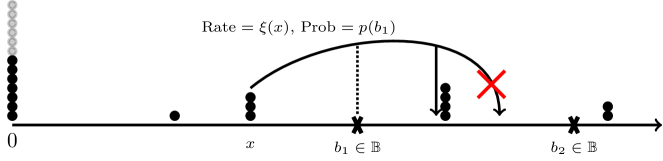
Figure 8: A possible jump in the continuous space TASEP $X(t)$. The jump occurs at rate $\xi(x)$. The moving particle overcomes the roadblock at $b_{1}$ with probability $p(b_{1})$, and joins the next stack because the particles preserve order.

We define the height function of the process $X(t)$ by

$$\mathcal{H}(t,\chi):=\#\{\text{particles }x_{i}\text{ at time $t$ such that }x_{i}\geq\chi\}.$$

The height function $\mathcal{H}(t,\chi)$ is almost surely weakly decreasing in $\chi\in\mathbb{R}_{>0}$ and $\lim_{\chi\rightarrow+\infty}\mathcal{H}(t,\chi)=0$. Additionally, it is very convenient to assume there are infinitely many particles at location $0$, so that $\mathcal{H}(t,0)\equiv+\infty$.

Let us now describe the regime in which the DGCG converges to the continuous space TASEP. Let $\varepsilon>0$ be a small parameter, and set $\beta_{t}=\varepsilon$ for all $t$. Scale the discrete time and space of the DGCG as

$$T=\lfloor\varepsilon^{-1}t\rfloor,\qquad N=\lfloor\varepsilon^{-1}\chi\rfloor.$$

To define the scaling of the $a_{i}$’s and the $\nu_{j}$’s, denote $\mathbf{B}^{\varepsilon}=\{\lfloor\varepsilon^{-1}b\rfloor,b\in\mathbf{B}\}\subset\mathbb{Z}_{\geq 1}$. Set

$$a_{1}=\xi(0),\qquad a_{j}=\xi(j\varepsilon),\qquad\nu_{j}=e^{-L\varepsilon},\qquad j\in\mathbb{Z}_{\geq 2}\setminus\mathbf{B}^{\varepsilon},$$ (2.3)

and

$$a_{i}=\xi(b),\qquad\nu_{i}=p(b),\qquad\textnormal{where $i=\lfloor\varepsilon^{-1}b\rfloor$ for $b\in\mathbf{B}$}.$$ (2.4)

In particular, all $\nu_{j}$ can be chosen nonnegative, and $\nu_{j}\to 1$ for almost all $j$. The roadblocks correspond to the indices $i$ such that $\nu_{i}<1$. Note that if $\xi(\cdot)$ is discontinuous at $0$ then the rate at which particles are added to the system from the infinite stack at $0$ is different from $\lim_{\chi\to 0+}\xi(\chi)$.

Theorem 2.7.

As $\varepsilon\to 0$ under the scalings described above, the DGCG height function converges to the one for the continuous space TASEP as $H_{T}(N)\to\mathcal{H}(t,\chi)$, in the sense of finite-dimensional distributions, jointly for all $(t,\chi)$.

Proof.

First, pass to the Poisson-type continuous time limit $\beta_{t}\equiv\beta\to 0$ in the DGCG, keeping the space and all other parameters $a_{i},\nu_{j}$ intact. Interpret this intermediate continuous time DGCG as a particle system on $\mathbb{Z}_{\geq 1}$, with $H_{T}(N)-H_{T}(N-1)$ particles at each $N\geq 2$, and infinitely many particles at $1$. Then new particles are added to the continuous time DGCG at rate $\beta^{-1}\frac{a_{1}\beta}{1+a_{1}\beta}=a_{1}+O(\beta)$ (see, e.g., the second line of Figure 6)

Now take the $\varepsilon$-dependent parameters $a_{i},\nu_{j}$ as above in the continuous time DGCG. We can couple this DGCG (for all $\varepsilon>0$) and continuous space TASEP such that they have the same number of particles at each time. This is possible since particles are added to both systems according to Poisson processes of rate $a_{1}=\xi(0)$. This coupling reduces the problem to finite particle systems, and one readily sees that all transition probabilities in DGCG converge to those in the continuous space TASEP (geometric random variables in DGCG become the exponential ones in the definition of the continuous space TASEP). ∎

Theorem 2.7 thus brings the Schur process type determinantal structure from the DGCG to the continuous space TASEP.

2.4 Comments

Let us make two detailed comments on the determinantal structure of the DGCG and the continuous space TASEP which is outlined above (detailed formulations of the determinantal structure are given in Section 3 below).

Limit as $q\to 0$ of previously known formulas.

First, we compare the existing methods to solve the $q$-deformations of the systems considered in the present paper. In the $q$-deformed setting, [CP16], [BP18], [BP18a] obtain formulas of two types:

1. The $q$-moments of the height function $\mathop{\mathbb{E}}q^{kH_{T}^{(q)}(N)}$, $k\in\mathbb{Z}_{\geq 1}$ (where $H_{T}^{(q)}$ is the height function of the $q$-dependent vertex model from Section 2.1), are expressed as $k$-fold nested contour integrals of elementary functions (for shortness, we do not specify the contours):

   $$\mathop{\mathbb{E}}q^{kH_{T}^{(q)}(N)}=\frac{q^{k(k-1)/2}}{(2\pi\sqrt{-1})^{2}}\oint\ldots\oint\frac{dw_{1}\ldots dw_{k}}{w_{1}\ldots w_{k}}\prod_{1\leq i<j\leq k}\frac{w_{i}-w_{j}}{w_{i}-qw_{j}}\\ \times\prod_{r=1}^{k}\left(\frac{1}{1-w_{r}/a_{1}}\prod_{j=2}^{N}\frac{a_{j}-\nu_{j}w_{r}}{a_{j}-w_{r}}\prod_{j=1}^{T}\frac{1+q\beta_{j}w_{r}}{1+\beta_{j}w_{r}}\right).$$

2. The $q$-Laplace transform $\mathop{\mathbb{E}}\bigr{(}(\zeta q^{H_{T}^{(q)}(N)};q)_{\infty}\bigl{)}^{-1}$ is written as a Fredholm determinant $\det(1+K_{\zeta}^{(q)})$ of a kernel which itself has a single contour integral representation:

   $$K_{\zeta}^{(q)}(w,w^{\prime})=\frac{1}{2\pi\sqrt{-1}}\int\Gamma(-u)\Gamma(1+u)(-\zeta)^{u}\frac{g(w)}{g(q^{u}w)}\frac{du}{q^{u}w-w^{\prime}},$$

   where $g(w)$ contains infinite $q$-Pochhammer symbols and is such that $g(w_{r})/g(qw_{r})$ is equal to the $r$-th term in the product in the above $q$-moment formula. Again, to shorten the exposition we do not specify the integration contour in $K_{\zeta}^{(q)}$ or the space on which this kernel acts.

Both the $q$-moment and the Fredholm determinantal formulas characterize the distribution of $H_{T}^{(q)}(N)$ uniquely. As $q\to 0$, the height functions $H_{T}^{(q)}(N)$ converge to the DGCG height function (denote it by $H_{T}^{(q=0)}(N)$ in this subsection). However, at $q=0$ both the observables $\mathop{\mathbb{E}}q^{kH_{T}^{(q)}(N)}$ and $\mathop{\mathbb{E}}\bigr{(}(\zeta q^{H_{T}^{(q)}(N)};q)_{\infty}\bigl{)}^{-1}$ provide almost no information about the distribution of $H_{T}^{(q=0)}(N)$.

In principle, before passing to the $q\to 0$ limit, one could invert the $q$-Laplace transform to express the distribution of $H_{T}^{(q)}(N)$ in a form which survives the $q\to 0$ transition. This inversion would involve taking an extra contour integral of the Fredholm determinant $\det(1+K_{\zeta}^{(q)})$ (e.g., see [BC14, Proposition 3.1.1]), and the result would contain $q$ in a very nontrivial manner. Instead of passing to the $q\to 0$ limit in this rather complicated Fredholm determinant, we utilize the connection of the $q$-dependent vertex model to the $q$-Whittaker processes found in [OP17] which easily survives the $q=0$ degeneration. In this way we relate $H_{T}^{(q=0)}(N)$ to Schur processes (which are the $q=0$ limits of the $q$-Whittaker processes), and then obtain asymptotic results by working with determinantal processes.

Joint distributions at different space locations.

Let us now discuss a limitation of the determinantal structure in describing the joint distributions of the height function $H_{T}(N)$ (or $\mathcal{H}(t,\chi)$) across different spatial locations.

The $q=0$ degeneration of the results of [OP17] implies a more general equality of joint distributions than (2.2). Let us describe the simplest nontrivial example. The joint distribution of $H_{T}(N_{1})$ and $H_{T}(N_{2})$, $N_{1}<N_{2}$, can be described as follows. First, we have $H_{T}(N_{1})\stackrel{{\scriptstyle d}}{{=}}Y_{N_{1}}(N_{1}-1;T)+N_{1}$, where $\vec{Y}$ is the mixed TASEP from Definition 2.5. Take the random configuration

$$\vec{Y}(N_{1}-1;T)=(Y_{1}(N_{1}-1;T)>Y_{2}(N_{1}-1;T)>\ldots),$$

and apply to it $N_{2}-N_{1}$ additional geometric steps with parameters $\nu_{N_{1}+1}/a_{N_{1}+1},\ldots,\nu_{N_{2}}/a_{N_{2}}$. Denote the resulting configuration by $\vec{Y}^{\prime}$. (In fact, the distribution of $\vec{Y}^{\prime}$ coincides with that of $\vec{Y}(N_{2}-1;T)$ from Definition 2.5, but note that the order of geometric and Bernoulli steps in $\vec{Y}^{\prime}$ is not the same as in $\vec{Y}(N_{2}-1;T)$.) Then we have

$$\left\{H_{T}(N_{1}),H_{T}(N_{2})\right\}\stackrel{{\scriptstyle d}}{{=}}\left\{Y_{N_{1}}(N_{1}-1;T)+N_{1},Y^{\prime}_{N_{2}}+N_{2}\right\}.$$

The joint distribution in the right-hand side is not given by a marginal of a Schur processes.

Joint distributions in TASEP corresponding to increasing both the particle’s number and the time are known as time-like (see, e.g., [DLSS91], [Fer08] about the terminology). Their asymptotic analysis is typically much harder than the one of the space-like joint distributions (which for TASEP are related to marginals of Schur processes). Asymptotic analysis of two-time time-like joint distribution in the last-passage percolation was performed recently in [Joh16], [Joh18]. (See also references to related non-rigorous and experimental work in the latter paper.) In the present work we do not consider joint distributions of the height function $H_{T}(N)$ involving more than one space location.

3 Determinantal structure via Schur processes

In this section we derive the determinantal structure of the DGCG and the continuous space TASEP. First, we recall the Schur processes and their determinantal structure (as applied to our concrete situation). Then, using Proposition 2.2 and Theorem 2.6, we obtain determinantal formulas for the DGCG model. A limit to continuous space then leads to determinantal formulas for the continuous space TASEP. Throughout the section the parameters $a_{i},\beta_{t},\nu_{j}$ are assumed to satisfy (1.1), with an additional restriction $\nu_{j}\geq 0$.

3.1 Schur processes

3.1.1 Young diagrams

A partition is a nonincreasing integer sequence of the form $\lambda=(\lambda_{1}\geq\ldots\geq\lambda_{\ell(\lambda)}>0)$. The number of nonzero parts $\ell(\lambda)$ (which must be finite) is called the length of a partition. Partitions are represented by Young diagrams, such that $\lambda_{1},\lambda_{2},\ldots$ denote the lengths of the successive rows. The column lengths of a Young diagram are denoted by $\lambda_{1}^{\prime}\geq\lambda_{2}^{\prime}\geq\ldots$. They form a transposed Young diagram $\lambda^{\prime}$. See Figure 9. The set of all partitions (equivalently, Young diagrams) is denoted by $\mathbb{Y}$.

Figure 9: A Young diagram $\lambda=(5,3,3,1,1,1)$ for which the transposed diagram is $\lambda^{\prime}=(6,3,3,1,1)$.

Let $\mu,\lambda$ be two Young diagrams. We say that $\lambda$ differs from $\mu$ by adding a horizontal strip (notation $\mu\prec\lambda$) iff $0\leq\lambda_{i}^{\prime}-\mu_{i}^{\prime}\leq 1$ for all $i$. We say that $\lambda$ differs by $\mu$ by adding a vertical strip (notation $\mu\prec^{\prime}\lambda$) iff $\mu^{\prime}\prec\lambda^{\prime}$.

3.1.2 Schur functions

For each Young diagram $\lambda$, let $s_{\lambda}$ be the corresponding Schur symmetric function [Mac95, Ch. I.3]. Evaluated at $N$ variables $u_{1},\ldots,u_{N}$ (where $N\geq\ell(\lambda)$ is arbitrary), $s_{\lambda}$ becomes the symmetric polynomial

$$s_{\lambda}(u_{1},\ldots,u_{N})=\frac{\det[u_{i}^{\lambda_{j}+N-j}]_{i,j=1}^{N}}{\det[u_{i}^{N-j}]_{i,j=1}^{N}}$$ (3.1)

If $N<\ell(\lambda)$, then $s_{\lambda}(u_{1},\ldots,u_{N})=0$ by definition. When all $u_{i}\geq 0$, the value $s_{\lambda}(u_{1},\ldots,u_{N})$ is also nonnegative. The Schur functions $s_{\lambda}$ form a linear basis in the algebra of symmetric functions $\Lambda$, where $\lambda$ runs over all possible Young diagrams.

Along with evaluating Schur functions at finitely many variables, we also need their general nonnegative specializations. That is, a nonnegative specialization is an algebra homomorphism $\rho\colon\Lambda\to\mathbb{C}$ such that $\rho(s_{\lambda})\geq 0$ for all Young diagrams $\lambda$. Nonnegative specializations are classified by the Edrei–Thoma theorem [Edr52], [Tho64] (also see, e.g., [BO16]). They depend on infinitely many real parameters $\vec{\alpha}=(\alpha_{1}\geq\alpha_{2}\ldots\geq 0)$, $\vec{\beta}=(\beta_{1}\geq\beta_{2}\geq\ldots\geq 0)$, and $\gamma\geq 0$, with $\sum_{i}(\alpha_{i}+\beta_{i})<\infty$, and are determined by the Cauchy summation identity

$$\sum_{\lambda\in\mathbb{Y}}s_{\lambda}(y_{1},\ldots,y_{n})\rho_{\vec{\alpha},\vec{\beta},\gamma}(s_{\lambda})=\prod_{j=1}^{n}\Biggl{(}e^{\gamma y_{j}}\prod_{i=1}^{\infty}\frac{1+\beta_{i}y_{j}}{1-\alpha_{i}y_{j}}\Biggr{)},$$ (3.2)

where $n\geq 1$ is arbitrary, and $y_{1},\ldots,y_{n}$ are regarded as formal variables. We will write $s_{\lambda}(\vec{\alpha};\vec{\beta};\gamma)=s_{\lambda}(\alpha_{1},\alpha_{2},\ldots;\beta_{1},\beta_{2},\ldots;\gamma)$ for $\rho_{\vec{\alpha},\vec{\beta},\gamma}(s_{\lambda})$ and will continue to use notation $s_{\lambda}(\alpha_{1},\ldots,\alpha_{m})$ for the substitution of the variables $\alpha_{1},\ldots,\alpha_{m}$ into $s_{\lambda}$ (which is the same as the specialization with finitely many $\alpha_{i}$’s and $\vec{\beta}=\vec{0}$, $\gamma=0$).

There are also skew Schur symmetric functions $s_{\lambda/\mu}$ which are defined through

$$s_{\lambda}(u_{1},\ldots,u_{N+M})=\sum_{\mu\in\mathbb{Y}}s_{\lambda/\mu}(u_{1},\ldots,u_{N})s_{\mu}(u_{N+1},\ldots,u_{N+M}).$$

The function $s_{\lambda/\mu}$ vanishes unless the Young diagram $\lambda$ contains $\mu$ (notation: $\lambda\supset\mu$). Skew Schur functions satisfy a skew generalization of the Cauchy summation identity:

$$\sum_{\nu\in\mathbb{Y}}s_{\nu/\mu}(x)s_{\nu/\lambda}(y)=\prod_{i,j}\frac{1}{1-x_{i}y_{j}}\sum_{\kappa\in\mathbb{Y}}s_{\mu/\kappa}(y)s_{\lambda/\kappa}(x),$$ (3.3)

where $\lambda,\mu$ are fixed and $x,y$ are two sets of variables. The specializations $s_{\lambda/\mu}(\vec{\alpha};\vec{\beta};\gamma)$ are well-defined and produce nonnegative numbers. The skew Schur functions $s_{\lambda/\mu}(a,0,\ldots;\vec{0};0)$ and $s_{\lambda/\mu}(\vec{0};\beta,0,\ldots;0)$ vanish unless, respectively, $\mu\prec\lambda$ and $\mu\prec^{\prime}\lambda$. For the specialization with all zeros we have we have $s_{\lambda/\mu}(\vec{0};\vec{0};0)=\mathbf{1}_{\lambda=\mu}$.

Taking the one-variable specializations $x=(\vec{0};\beta,0,\ldots;0)$ and $y=(a,0,\ldots;\vec{0};0)$ in (3.3), we get the identity

$$\sum_{\nu\in\mathbb{Y}}s_{\nu/\mu}(\vec{0};\beta;0)s_{\nu/\lambda}(a;\vec{0};0)=(1+a\beta)\sum_{\kappa\in\mathbb{Y}}s_{\mu/\kappa}(a;\vec{0};0)s_{\lambda/\kappa}(\vec{0};\beta;0),$$ (3.4)

where $a,\beta\geq 0$ are real numbers. We refer to, e.g., [Mac95, Ch I] for further details on ordinary and skew Schur functions.

3.1.3 A field of Young diagrams

Recall the discrete parameters $\{a_{i}\}_{i\geq 1}$, $\{\nu_{i}\}_{i\geq 2}$, and $\{\beta_{i}\}_{i\geq 1}$ (Definition 1.2), and fix $N\in\mathbb{Z}_{\geq 1}$. Consider a random field of Young diagrams, that is, a probability distribution on an array of Young diagrams $\{\lambda^{(T,K)}\}_{T,K\in\mathbb{Z}_{\geq 0}}$ (cf. Figure 11) with the following properties:

1. (bottom boundary condition) For all $T\geq 0$ we have $\lambda^{(T,0)}=\varnothing$.

2. (left boundary condition) For all $M\in\mathbb{Z}_{\geq 0}$, the joint distribution of the Young diagrams $\lambda^{(0,K)}$, $0\leq K\leq M$, at the left boundary is given by the following ascending Schur process:

   $$\mathop{\mathrm{Prob}}\bigl{(}\lambda^{(0,0)},\lambda^{(0,1)},\ldots,\lambda^{(0,M)}\bigr{)}=\frac{1}{Z}s_{\lambda^{(0,1)}}(a_{1})\\ \times s_{\lambda^{(0,2)}/\lambda^{(0,1)}}(a_{2})\ldots s_{\lambda^{(0,M)}/\lambda^{(0,M-1)}}(a_{M})s_{\lambda^{(0,M)}}\Bigl{(}\frac{\nu_{2}}{a_{2}},\ldots,\frac{\nu_{N}}{a_{N}}\Bigr{)},$$ (3.5)

   where $Z$ is the normalizing constant. In particular, this implies that along the left edge each two consecutive Young diagrams $\lambda^{(0,j)}$ and $\lambda^{(0,j+1)}$ almost surely differ by adding a horizontal strip. In particular, $\ell(\lambda^{(0,j)})\leq j$.

3. (conditional distributions) For any $i,j\in\mathbb{Z}_{\geq 1}$ consider the quadruple of neighboring Young diagrams $\kappa=\lambda^{(i-1,j-1)}$, $\lambda=\lambda^{(i,j-1)}$, $\mu=\lambda^{(i-1,j)}$, and $\nu=\lambda^{(i,j)}$ (we use these notations to shorten the formulas; cf. Figure 10). The conditional distributions in this quadruple are as follows:

   $$\begin{split}&\mathop{\mathrm{Prob}}\bigl{(}\nu\mid\lambda^{(p,q)}\colon\textnormal{$p\leq i-1,q\geq j-1$ or $p\geq i-1$, $q\leq j-1$}\bigr{)}\\ &\hskip 50.0pt=\mathop{\mathrm{Prob}}(\nu\mid\lambda,\mu)=\frac{s_{\nu/\mu}(\vec{0};\beta_{i},0,\ldots;0)s_{\nu/\lambda}(a_{j},0,\ldots;\vec{0};0)}{Z_{u}^{(i,j)}};\\ &\mathop{\mathrm{Prob}}\bigl{(}\kappa\mid\lambda^{(p,q)}\colon\textnormal{$p\leq i-1,q\geq j-1$ or $p\geq i-1$, $q\leq j-1$}\bigr{)}\\ &\hskip 50.0pt=\mathop{\mathrm{Prob}}(\kappa\mid\lambda,\mu)=\frac{s_{\mu/\kappa}(a_{j},0,\ldots;\vec{0};0)s_{\lambda/\kappa}(\vec{0};\beta_{j},0,\ldots;0)}{Z_{\ell}^{(i,j)}},\end{split}$$ (3.6)

   where $Z_{u}^{(i,j)},Z_{\ell}^{(i,j)}$ are normalizing constants. In particular, $\mu\prec^{\prime}\nu$, $\kappa\prec^{\prime}\lambda$, $\kappa\prec\mu$, and $\lambda\prec\nu$ almost surely, and this implies that $\ell(\lambda^{(i,j)})\leq j$ for all $i,j$. The skew Cauchy identity (3.4) implies that $Z_{u}^{(i,j)}=(1+\beta_{i}a_{j})Z_{\ell}^{(i,j)}$.

	$\mu$	$\prec^{\prime}$	$\nu$
$\scriptstyle(a_{j})$	$\prec$		$\prec$
	$\kappa$	$\prec^{\prime}$	$\lambda$
		$\scriptstyle(\beta_{i})$

Figure 10: A quadruple of Young diagrams in the field $\lambda^{(T,K)}$.

The above conditions 1–3 do not define a field $\lambda^{(T,K)}$ uniquely. Namely, while (3.6) specifies the marginal distributions of $\kappa$ and $\nu$ (given $\mu,\lambda$), it does not specify the joint distribution of $(\kappa,\nu)$ (given $\mu,\lambda$). It is possible to specify this joint distribution such that

1. the field $\{\lambda^{(T,K)}\}_{T,K\in\mathbb{Z}_{\geq 0}}$ is well-defined (i.e., satisfies 1–3);

2. the scalar field $\{\lambda^{(T,K)}_{K}\}_{T,K\in\mathbb{Z}_{\geq 0}}$ of the last parts of the partitions is marginally Markovian in the sense that its distribution does not depend on the distribution of the other parts of the partitions.

There are two main constructions of the field $\lambda^{(T,K)}$ satisfying 1–3 and with marginally Markovian last parts. One involves the Robinson-Schensted-Knuth (RSK) correspondence and follows [O’C03a], [O’C03], see also [DW08, Case B], and another construction can be read off [BF14]. The latter construction postulates that the joint distribution of $\kappa,\nu$ given $\lambda,\mu$ is essentially the product of the marginal distributions (3.6), unless this violates conditions in Figure 10 (in which case the product formula has to be corrected). The RSK construction involves more complicated combinatorial rules for stitching together the marginal distributions of $\kappa$ and $\nu$. Either of these constructions of $\{\lambda^{(T,K)}\}$ works for our purposes, and we do not discuss further details. The marginally Markovian evolution of the last parts $\lambda^{(T,K)}_{K}$ is the discrete time TASEP with mixed geometric and Bernoulli steps which we describe in Section 2.2. In the rest of this section we refer to $\{\lambda^{(T,K)}\}$ simply as the random field of Young diagrams.

Lemma 3.1.

For any fixed $T,K\in\mathbb{Z}_{\geq 0}$ the marginal distribution of the random Young diagram $\lambda=\lambda^{(T,K)}$ is given by the Schur measure

$$\mathop{\mathrm{Prob}}(\lambda)=\frac{1}{Z}s_{\lambda}(a_{1},\ldots,a_{K})s_{\lambda}\Bigl{(}\frac{\nu_{2}}{a_{2}},\ldots,\frac{\nu_{N}}{a_{N}};\beta_{1},\ldots,\beta_{T};0\Bigr{)}.$$ (3.7)

The normalizing constant in (3.7) is given by (cf. (3.2))

$$Z=\prod_{i=1}^{K}\Biggl{(}\prod_{j=2}^{N}\frac{1}{1-a_{i}\nu_{j}/a_{j}}\prod_{j=1}^{T}(1+a_{i}\beta_{j})\Biggr{)}.$$

Idea of proof of Lemma 3.1.

Follows by repeatedly applying the skew Cauchy identity (3.4) and arguing by induction on adding a box to grow the $T\times K$ rectangle. The additional specialization $(\nu_{2}/a_{2},\ldots,\nu_{N}/a_{N})$ comes from the left boundary condition in the field $\{\lambda^{(T,K)}\}$. ∎

The notion of random fields of Young diagrams was introduced recently [BM18], [BP17] to capture properties of coupled Schur processes. This concept extends the work started with [OP13], [BP16a], and earlier applications of Robinson-Schensted-Knuth correspondences to particle systems [Joh00], [O’C03a], [O’C03]. In the next part we consider down-right joint distributions in the field $\lambda^{(K,T)}$ which are given by more general Schur processes.

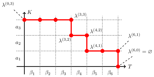
Figure 11: A graphical representation of the field $\lambda^{(T,K)}$ of Young diagrams, and a down-right path.

3.1.4 Schur processes and correlation kernels

Here we recall (at an appropriate level of generality) the definition and the correlation kernel for Schur processes from [OR03]. Fix the parameters $N$ and $\{a_{i}\}$, $\{\nu_{i}\}$, $\{\beta_{i}\}$. Take a down-right path $\{(T_{j},K_{j})\}_{j=1}^{\ell}$, that is,

$$K_{1}\geq\ldots\geq K_{\ell}=0,\qquad 0=T_{1}\leq\ldots\leq T_{\ell},$$ (3.8)

and, moreover, assume that the points $(T_{j},K_{j})$ are pairwise distinct. A Schur process associated with this data is a probability distribution on sequences $(\lambda;\mu)$ of Young diagrams (see Figure 11 for an illustration)

$$\varnothing=\mu^{(1)}\subset\lambda^{(1)}\supset\mu^{(2)}\subset\lambda^{(2)}\supset\mu^{(3)}\subset\ldots\subset\lambda^{(\ell-1)}\supset\mu^{(\ell)}=\varnothing$$ (3.9)

with probability weights

$$\mathop{\mathrm{Prob}}(\lambda;\mu)=\frac{1}{Z}s_{\lambda^{(1)}/\mu^{(1)}}\Bigl{(}\frac{\nu_{2}}{a_{2}},\ldots,\frac{\nu_{N}}{a_{N}}\Bigr{)}s_{\lambda^{(1)}/\mu^{(2)}}(a_{(K_{2},K_{1}]})s_{\lambda^{(2)}/\mu^{(2)}}(\beta_{(0,T_{2}]})\ldots\\ \times s_{\lambda^{(\ell-1)}/\mu^{(\ell-1)}}(\beta_{(T_{\ell-1},T_{\ell}]})s_{\lambda^{(\ell-1)}/\mu^{(\ell)}}(a_{(0,K_{\ell-1}]}).$$ (3.10)

Here $a_{(u,v]}$ stands for the specialization $(a_{u+1},\ldots,a_{v};\vec{0};0)$ corresponding to the vertical direction of the down-right path, and $\beta_{(u,v]}$ means $(\vec{0};\beta_{u+1},\ldots,\beta_{v};0)$ (this corresponds to the horizontal direction). Note that some of these specializations can be empty. The normalizing constant in (3.10) can be readily computed using the Cauchy identities.

As shown in [OR03], the Schur process (3.10) can be interpreted as a determinantal random point process whose correlation kernel is expressed as a double contour integral. (We refer to, e.g., [Sos00], [HKPV06], [Bor11], for general definitions related to determinantal processes.) To recall the result of [OR03], consider the particle configuration

$$\bigl{\{}\lambda^{(i)}_{j}-j\colon i=1,\ldots,\ell-1,\ j=1,2,\ldots\bigr{\}}\subset\underbrace{\mathbb{Z}\times\ldots\times\mathbb{Z}}_{\textnormal{$\ell-1$ times}}$$ (3.11)

corresponding to a sequence (3.9) (where we sum over all the $\mu^{(j)}$’s). The configurations $\lambda^{(i)}_{j}-j$, $j\geq 1$, are infinite and are densely packed at $-\infty$ (i.e., each partition $\lambda^{(i)}$ is appended infinitely many zeroes). Then, for any $m$ and any pairwise distinct locations $(r_{p},x_{p})$, $p=1,\ldots,m$, where $1\leq r_{p}\leq\ell-1$ and $x_{p}\in\mathbb{Z}$, we have

$$\mathbb{P}\Bigl{(}\textnormal{there are points of the configuration \eqref{eq:particle_configuration_for_Schur_process} at each of the locations $(r_{p},x_{p})$}\Bigr{)}\\ =\det\left[\mathsf{K}_{\mathsf{SP}}(r_{p},x_{p};r_{q},x_{q})\right]_{p,q=1}^{m}.$$

The kernel $\mathsf{K}_{\mathsf{SP}}$ has the form

$$\mathsf{K}_{\mathsf{SP}}(i,x;j,y)=\frac{1}{(2\pi{\mathbf{i}\mkern 1.0mu})^{2}}\oint\oint\frac{dz\,dw}{z-w}\frac{w^{y}}{z^{x+1}}\frac{\Phi(i,z)}{\Phi(j,w)},$$ (3.12)

where

$$\Phi(i,z)=\prod_{n=2}^{N}\frac{1}{1-z\nu_{n}/a_{n}}\prod_{t=1}^{T_{i}}(1+\beta_{t}z)\prod_{k=1}^{K_{i}}(1-z^{-1}a_{k}).$$

The integration contours in (3.12) are positively oriented simple closed curves around $0$ satisfying $|z|>|w|$ for $i\leq j$ and $|z|<|w|$ for $i>j$. Moreover, on the contours it must be $|z|<a_{n}/\nu_{n}$, $a_{k}<|w|<\beta_{t}^{-1}$ for all $n,t,k$ entering the products in (3.12). In particular, the $w$ contour should encircle the $a_{k}$’s. Thus, we have the following determinantal structure in the field $\{\lambda^{(T,K)}\}$:

Proposition 3.2.

For any $m\in\mathbb{Z}_{\geq 1}$ and any collection of pairwise distinct integer triplets $\{(T_{i},K_{i},x_{i})\}_{i=1}^{m}$ such that $K_{1}\geq\ldots\geq K_{m}\geq 0$, $0\leq T_{1}\leq\ldots\leq T_{m}$, we have

$$\mathop{\mathrm{Prob}}\bigl{(}\textnormal{for all $i$, the configuration $\{\lambda^{(T_{i},K_{i})}_{j}-j\}_{j\geq 1}\subset\mathbb{Z}$ contains a particle at $x_{i}$}\bigl{)}\\ =\det[\mathsf{K}(T_{p},K_{p},x_{p};T_{q},K_{q},x_{q})]_{p,q=1}^{m},$$ (3.13)

where the kernel is given by

$$\mathsf{K}(T,K,x;T^{\prime},K^{\prime},x^{\prime})=\frac{1}{(2\pi{\mathbf{i}\mkern 1.0mu})^{2}}\oint\oint\frac{dz\,dw}{z-w}\frac{w^{x^{\prime}}}{z^{x+1}}\prod_{n=2}^{N}\frac{1-w\nu_{n}/a_{n}}{1-z\nu_{n}/a_{n}}\\ \times\frac{\prod_{t=1}^{T}(1+\beta_{t}z)}{\prod_{t=1}^{T^{\prime}}(1+\beta_{t}w)}\frac{\prod_{k=1}^{K}(1-z^{-1}a_{k})}{\prod_{k=1}^{K^{\prime}}(1-w^{-1}a_{k})}.$$ (3.14)

The contours are positively oriented simple closed curves around $0$ such that $w$ also encircles the $a_{k}$’s, $|z|>|w|$ for $T\leq T^{\prime}$, and $|z|<|w|$ for $T>T^{\prime}$. Moreover, on the contours it must be $|z|<a_{n}/\nu_{n}$, $|w|<\beta_{t}^{-1}$ for all $t,n$.

Remark 3.3.

In the description of the integration contours in Proposition 3.2 we silently assumed that the parameters $a_{i},\beta_{t},\nu_{j}$ satisfy certain restrictions such that the contours exist. In Proposition 3.4 below we deform the contours and lift these restrictions when $K=K^{\prime}=N$ (this holds when we apply the Schur process structure to DGCG).

3.1.5 Particles at the edge and Fredholm determinants

The joint distribution of the last parts of the partitions $\{\lambda^{(T_{i},K_{i})}_{K_{i}}\}$ (which evolve in a marginally Markovian way) for $(T_{i},K_{i})$ along a down-right path can be written in terms of a Fredholm determinant.

Let us first recall Fredholm determinants on an abstract discrete space $\mathfrak{X}$. Let $\mathsf{K}(i,i^{\prime})$, $i,i^{\prime}\in\mathfrak{X}$, be a kernel on this space. We define the Fredholm determinant of $\mathbf{1}+z\mathsf{K}$, $z\in\mathbb{C}$, as the infinite series

$$\det(1+z\mathsf{K})_{\mathfrak{X}}=1+\sum_{r=1}^{\infty}\frac{z^{r}}{r!}\sum_{i_{1}\in\mathfrak{X}}\ldots\sum_{i_{r}\in\mathfrak{X}}\det\left[\mathsf{K}(i_{p},i_{q})\right]_{p,q=1}^{r}.$$ (3.15)

One may view (3.15) as a formal series, but in our setting this series will converge numerically. Details on Fredholm determinants may be found in [Sim05] or [Bor10].

Fix a down-right path $\{(T_{i},K_{i})\}_{i=1}^{\ell}$ as in (3.8), and consider the space

$$\mathfrak{X}=\bigcup_{i=1}^{\ell-1}\bigl{(}\{T_{i}\}\times\{K_{i}\}\times\mathbb{Z}\bigr{)}.$$

According to Proposition 3.2, let us view $\{\lambda^{(T_{i},K_{i})}_{j}-j\colon i=1,\ldots,\ell-1,\;j=1,2,\ldots\}$ as a determinantal point process on $\mathfrak{X}$ with correlation kernel $\mathsf{K}(Y;Y^{\prime})=\mathsf{K}(T,T,y;T^{\prime},K^{\prime},y^{\prime})$, where $Y=(T,K,y),Y^{\prime}=(T^{\prime},K^{\prime},y^{\prime})\in\mathfrak{X}$. Fix $\vec{y}=(y_{1},\ldots,y_{\ell-1})\in\mathbb{Z}^{\ell-1}$ and interpret

$$\mathop{\mathrm{Prob}}\Bigl{(}\lambda^{(T_{i},K_{i})}_{K_{i}}-K_{i}>y_{i}\colon i=1,\ldots,\ell-1\Bigr{)}$$

as the probability that the random point configuration $\mathfrak{X}$ corresponding to our determinantal process has no particles in the set

$$\mathfrak{X}_{\vec{y}}:=\bigcup_{i=1}^{\ell-1}\bigl{(}\left\{T_{i}\right\}\times\left\{K_{i}\right\}\times\left\{-K_{i},-K_{i}+1,\ldots,y_{i}-1,y_{i}\right\}\bigr{)}\subset\mathfrak{X}.$$

This probability can be written (e.g., see [Sos00]) as the Fredholm determinant

$$\det\left(\mathbf{1}-\chi_{\vec{y}}\mathsf{K}\chi_{\vec{y}}\right)_{\mathfrak{X}},$$

where $\chi_{\vec{y}}(T_{i},K_{i},x)=\mathbf{1}_{-K_{i}\leq x\leq y_{i}}$, $i=1,\ldots,\ell-1$, is the indicator of $\mathfrak{X}_{\vec{y}}\subset\mathfrak{X}$ viewed as a projection operator acting on functions.

In particular, in the one-point case we get the following Fredholm determinant:

$$\mathop{\mathrm{Prob}}\bigl{(}\lambda^{(T,K)}_{K}-K>y\bigr{)}=\det(\mathbf{1}-\mathsf{K}(T,K,\cdot;T,K,\cdot))_{\{-K,-K+1,\ldots,y-1,y\}}\\ =1+\sum_{m=1}^{\infty}\frac{(-1)^{m}}{m!}\sum_{x_{1}=-K}^{y}\ldots\sum_{x_{m}=-K}^{y}\det[\mathsf{K}(T,K,x_{p};T,K,x_{q})]_{p,q=1}^{m},$$

where the last equality is the series expansion of the Fredholm determinant.

3.2 Determinantal structure of DGCG

Let us now apply the formalism of Schur processes to the DGCG model. We will us the kernel $\mathsf{K}$ (3.14) with $K=K^{\prime}=N$ and different integration contours. That is, define

$$\begin{split}&\mathsf{K}_{N}(T,x;T^{\prime},x^{\prime}):=-\frac{\mathbf{1}_{T>T^{\prime}}\mathbf{1}_{x\geq x^{\prime}}}{2\pi{\mathbf{i}\mkern 1.0mu}}\oint\frac{\prod_{t=T^{\prime}+1}^{T}(1+\beta_{t}z)}{z^{x-x^{\prime}+1}}\,dz\\ &\hskip 20.0pt+\frac{1}{(2\pi{\mathbf{i}\mkern 1.0mu})^{2}}\oint\oint\frac{dz\,dw}{z-w}\frac{w^{x^{\prime}+N}}{z^{x+N+1}}\prod_{n=2}^{N}\frac{1-w\nu_{n}/a_{n}}{1-z\nu_{n}/a_{n}}\frac{\prod_{t=1}^{T}(1+\beta_{t}z)}{\prod_{t=1}^{T^{\prime}}(1+\beta_{t}w)}\prod_{k=1}^{N}\frac{a_{k}-z}{a_{k}-w},\end{split}$$ (3.16)

where $T,T^{\prime}\in\mathbb{Z}_{\geq 0}$ and $x,x^{\prime}\in\mathbb{Z}_{\geq-N}$. In the single integral the contour is a small positively oriented circle around $0$, and the contours in the double integral satisfy:

1. the $z$ contour is a small positively oriented circle around $0$ which must be to the left of all points $a_{n}/\nu_{n}$;

2. the $w$ contour is a positively oriented simple closed curve around all the $a_{k}$’s which stays to the right of zero, all points $-\beta_{t}^{-1}$, and the $z$ contour.

Proposition 3.4.

The integration contours in (3.16) exist for all choices of parameters $a_{i}>0$, $\beta_{t}>0$, and $\nu_{j}\in[0,1)$. Moreover, $\mathsf{K}_{N}(T,x;T^{\prime},x^{\prime})=\mathsf{K}(T,N,x;T^{\prime},N,x^{\prime})$, where the latter is given in (3.14).

In other words, the deformation of contours from $\mathsf{K}(T,N,x;T^{\prime},N,x^{\prime})$ to $\mathsf{K}_{N}(T,x;T^{\prime},x^{\prime})$ provides an analytic continuation of the kernel to the full range of parameters $a_{i}>0$, $\beta_{t}>0$, $\nu_{j}\in[0,1)$.

Proof of Proposition 3.4.

The existence of the contours is straightforward. Let us explain how to deform the contours in $\mathsf{K}(T,N,x;T^{\prime},N,x^{\prime})$ to get the desired result. First, note that the integrand is regular at $w=0$ for $x^{\prime}\geq-N$. Depending on the relative order of $T$ and $T^{\prime}$, perform the following contour deformations:

1. For $T\leq T^{\prime}$, the $w$ contour is inside the $z$ one in (3.14). Drag the $z$ contour through the $w$ one, and turn $z$ into a small circle around $0$. The $w$ contour then needs to encircle only $\{a_{i}\}$ and not zero, as desired. This deformation of the contours results in a single integral of the residue at $z=w$ over the new $w$ contour, but since this contour does not include zero, the single integral vanishes.

2. When $T>T^{\prime}$, the $z$ contour is inside the $w$ one in (3.14). Make $z$ a small circle around $0$, then drag the $w$ contour through the $z$ one, and have the $w$ contour encircle $\{a_{i}\}$ and not zero. This deformation brings a single integral of the residue at $w=z$ over the new $z$ contour, and this is precisely the single integral we get in (3.16).

These contour deformations lead to the kernel $\mathsf{K}_{N}$. ∎

Fix $\ell\geq 1$ and $0\leq T_{1}\leq\ldots\leq T_{\ell}$, and define a determinantal point process $\mathfrak{L}_{N,\ell}$ on $\mathfrak{X}:=\mathbb{Z}_{\geq-N}\times\{T_{1},\ldots,T_{\ell}\}$ as follows. For any $m\geq 1$ and $m$ pairwise distinct points $(x_{i},t_{i})\in\mathfrak{X}$, set

$$\mathop{\mathrm{Prob}}\bigl{(}\textnormal{the random configuration $\mathfrak{L}_{N,\ell}$ contains all points $(x_{i},t_{i})$, $i=1,\ldots,m$}\bigr{)}\\ =\det\left[\mathsf{K}_{N}(t_{i},x_{i};t_{j},x_{j})\right]_{i,j=1}^{m}.$$ (3.17)

In other words, $\mathfrak{L}_{N,\ell}$ is the $\mathbb{Z}_{\geq-N}$-part of the determinantal process $\lambda^{(i)}_{j}-j$ coming from the Schur process as in Section 3.1.4 corresponding to the down-right path $\{(T_{j},K_{j})\}=\{(T_{j},N)\}$. See Figure 12 for an illustration.

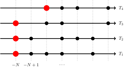
Figure 12: An example of a configuration of $\mathfrak{L}_{N,4}$. The leftmost particles are highlighted.

Theorem 3.5.

With the above notation, the joint distribution of the height function of the DGCG

$$\{H_{T_{j}}(N+1)-N\}_{j=1}^{\ell}$$

coincides with the joint distribution of the leftmost points of the determinantal point process $\mathfrak{L}_{N,\ell}$ on $\mathbb{Z}_{\geq-N}\times\{T_{1},\ldots,T_{\ell}\}$.

Proof.

We know from Proposition 2.2 and Theorem 2.6 that

$$\{H_{T_{j}}(N+1)-N\}_{j=1}^{\ell}\stackrel{{\scriptstyle d}}{{=}}\{Y_{N}(N-1;T_{j})\}_{j=1}^{\ell},$$

where $\vec{Y}(N-1;T)$ is the mixed TASEP of Definition 2.5. If we connect $\vec{Y}(N-1;T)$ to a field of random Young diagrams, then the desired statement would follow from the determinantal structure of the Schur process described in Section 3.2.

The desired connection of the mixed TASEP with particle-dependent inhomogeneity to Schur processes is in well-known and follows from the column Robinson-Schensted-Knuth (RSK) correspondences (see [Ful97], [Sta01] for details on RSK, and, e.g., [Joh00], [O’C03], [WW09] for probabilistic applications of RSK to TASEPs) or, alternatively, from the results of [BF14]. The precise connection reads as follows. For any down-right path $\{(T_{j},K_{j})\}_{j=1}^{\ell}$ (3.8) we have the equality of the following joint distributions:

$$\left\{Y_{K_{j}}(N-1;T_{j})+K_{j}\right\}_{j=1}^{\ell-1}\stackrel{{\scriptstyle d}}{{=}}\bigl{\{}\lambda^{(T_{j},K_{j})}_{K_{j}}\bigr{\}}_{j=1}^{\ell-1},$$ (3.18)

where $\vec{Y}$ is the mixed TASEP, and $\{\lambda(T,K)\}$ is the random field from Section 3.1.3. In particular, the distribution of each particle $Y_{K}(N-1;T)$ in the mixed TASEP is the same as of $\lambda_{K}-K$, where $\lambda_{K}$ is the last part of a random partition $\lambda$ chosen from the Schur measure $\propto s_{\lambda}(a_{1},\ldots,a_{K};\vec{0};0)s_{\lambda}(\nu_{2}/a_{2},\ldots,\nu_{N}/a_{N};\beta_{1},\ldots,\beta_{T};0)$.

Taking $K_{j}\equiv N$ in (3.18) and using Proposition 3.2 (together with Proposition 3.4 for the contour deformation), we arrive at the claim. ∎

In particular, for $\ell=1$ Theorem 3.5 implies the following Fredholm determinantal expression for the distribution of the random variable $H_{T}(N+1)$:

$$\mathop{\mathrm{Prob}}\bigl{(}H_{T}(N+1)-N>y\bigr{)}=\det(\mathbf{1}-\mathsf{K}_{N}(T,\cdot;T,\cdot))_{\left\{-N,-N+1,\ldots,y-1,y\right\}}\\ =1+\sum_{m=1}^{\infty}\frac{(-1)^{m}}{m!}\sum_{x_{1}=-N}^{y}\ldots\sum_{x_{m}=-N}^{y}\det[\mathsf{K}_{N}(T,x_{i};T,x_{j})]_{i,j=1}^{m}.$$ (3.19)

The second equality is the series expansion of the Fredholm determinant, see Section 3.1.5.

3.3 Determinantal structure of continuous space TASEP

Let us now describe the determinantal structure of the continuous space TASEP which follows by taking the continuous space scaling of the DGCG results. By $N+\mathfrak{L}_{N,\ell}$ denote the shift of the determinantal process $\mathfrak{L}_{N,\ell}$ from Section 3.2 by $N$ to the right.

Theorem 3.6.

As $\varepsilon\to 0$ and under the scaling described in defined Section 2.3, $N+\mathfrak{L}_{N,\ell}$ converges in the sense of finite dimensional distributions to a determinantal point process $\widetilde{\mathfrak{L}}_{\ell}$ on $\mathbb{Z}_{\geq 0}\times\{t_{1},\ldots,t_{\ell}\}$ (where $T_{i}=\lfloor\varepsilon^{-1}t_{i}\rfloor$) with the kernel 

$$\mathcal{K}(t,x;t^{\prime},x^{\prime})=-\mathbf{1}_{t>t^{\prime}}\mathbf{1}_{x\geq x^{\prime}}\frac{(t-t^{\prime})^{x-x^{\prime}}}{(x-x^{\prime})!}$$

$$\hskip 30.0pt+\frac{1}{(2\pi{\mathbf{i}\mkern 1.0mu})^{2}}\oint\oint\frac{dwdz}{z-w}\frac{w^{x^{\prime}}}{z^{x+1}}\exp\biggl{\{}tz-t^{\prime}w+L\int\limits_{0}^{\chi}\left(\frac{w}{\xi(u)-w}-\frac{z}{\xi(u)-z}\right)du\biggr{\}}$$ (3.20)

$$\hskip 190.0pt\times\frac{(\xi(0)-z)}{(\xi(0)-w)}\prod\limits_{b\in\mathbf{B}\colon b<\chi}\frac{\xi(b)-p(b)w}{\xi(b)-p(b)z}\cdot\frac{\xi(b)-z}{\xi(b)-w}.$$

The $z$ contour is a small positively oriented circle around $0$ which must be to the left of all points $\xi(y),$ $y\in[0,\chi]$. The $w$ contour is a positively oriented simple closed curve around all points $\xi(y),$ $y\in[0,\chi]$ which is also to the right of the $z$ contour.

Correspondingly, the joint distribution $\left\{\mathcal{H}(t_{i},\chi)\right\}_{i=1}^{\ell}$ of the continuous space TASEP height function coincides with the joint distribution of the leftmost particles of $\widetilde{\mathfrak{L}}_{\ell}$.

Proof.

The second part of the claim (that $\mathcal{H}(t_{i},\chi)$ are the leftmost points of $\widetilde{\mathfrak{L}}_{\ell}$) follows from the first part together with Theorem 2.7. Thus, it suffices to establish the convergence of the correlation kernels $\mathsf{K}_{N}$ (3.16) to $\mathcal{K}$ (3.20) (which would imply the convergence of determinantal point processes in the sense of finite dimensional distributions since those are completely determined by the correlation kernels, cf. [Sos00]).

Because of the shift $N+\mathfrak{L}_{N,\ell}$ we first subtract $N$ from $x,x^{\prime}$ in $\mathsf{K}_{N}$, and then scale $a_{i},\nu_{j},\beta_{t},T,N$ depending on $\varepsilon$. First, observe that the single integral in (3.16) converges to the first term in (3.20):

$$-\frac{\mathbf{1}_{T>T^{\prime}}\mathbf{1}_{x\geq x^{\prime}}}{2\pi{\mathbf{i}\mkern 1.0mu}}\oint\frac{\prod_{t=T^{\prime}+1}^{T}(1+\beta_{t}z)}{z^{x-x^{\prime}+1}}\,dz\to-\frac{\mathbf{1}_{t>t^{\prime}}\mathbf{1}_{x\geq x^{\prime}}}{2\pi{\mathbf{i}\mkern 1.0mu}}\oint\frac{e^{z(t-t^{\prime})}dz}{z^{x-x^{\prime}+1}}=-\mathbf{1}_{t>t^{\prime}}\mathbf{1}_{x\geq x^{\prime}}\frac{(t-t^{\prime})^{x-x^{\prime}}}{(x-x^{\prime})!}.$$

Next, let us look at the double integrals. Under our scaling the integration contours readily match, so it remains to show the convergence of the integrands. Keep $\dfrac{w^{x^{\prime}}}{z^{x+1}(z-w)}$, and also separate the factors $\dfrac{a_{1}-z}{a_{1}-w}=\dfrac{\xi(0)-z}{\xi(0)-w}$ from the product over $k=1,\ldots,N$. These factors do not change with $\varepsilon$. Consider the limit as $\varepsilon\to 0$ of the remaining factors in the integrand. We have

$$\frac{\prod_{t=1}^{T}(1+\beta_{t}z)}{\prod_{t=1}^{T^{\prime}}(1+\beta_{t}w)}=\frac{(1+\varepsilon z)^{\lfloor\varepsilon^{-1}t\rfloor}}{(1+\varepsilon w)^{\lfloor\varepsilon^{-1}t^{\prime}\rfloor}}\to e^{tz-t^{\prime}w}.$$

In the product

$$\prod_{n=2}^{N}\frac{a_{n}-w\nu_{n}}{a_{n}-w}\cdot\frac{a_{n}-z}{a_{n}-z\nu_{n}}$$

consider separately the factors corresponding to $n\in\mathbf{B}^{\varepsilon}$. We obtain for all sufficiently small $\varepsilon$:

$$\prod_{2\leq n\leq\lfloor\varepsilon^{-1}\chi\rfloor,\,n\in\mathbf{B}^{\varepsilon}}\frac{a_{n}-w\nu_{n}}{a_{n}-w}\cdot\frac{a_{n}-z}{a_{n}-z\nu_{n}}=\prod_{b\in\mathbf{B}\colon b<\chi}\frac{\xi(b)-p(b)w}{\xi(b)-w}\cdot\frac{\xi(b)-z}{\xi(b)-p(b)z},$$

and these factors also do not change with $\varepsilon$ (there are finitely many roadblocks on $[0,\chi)$). Finally,

$$\prod_{2\leq n\leq N,\,n\notin\mathbf{B}^{\varepsilon}}\frac{a_{n}-w\nu_{n}}{a_{n}-w}=\exp\Biggl{\{}\sum_{2\leq n\leq\lfloor\varepsilon^{-1}\chi\rfloor,\,n\notin\mathbf{B}^{\varepsilon}}\log\biggl{(}\frac{\xi(n\varepsilon)-we^{-L\varepsilon}}{\xi(n\varepsilon)-w}\biggr{)}\Biggr{\}}\\ =\exp\Biggl{\{}\varepsilon L\sum_{2\leq n\leq\lfloor\varepsilon^{-1}\chi\rfloor,\,n\notin\mathbf{B}^{\varepsilon}}\biggl{(}\frac{w}{\xi(n\varepsilon)-w}+O(\varepsilon^{2})\biggl{)}\Biggr{\}}\to\exp\biggl{\{}L\int_{0}^{\chi}\frac{w}{\xi(u)-w}\,du\biggr{\}},$$

because the exclusion of finitely many points $n\in\mathbf{B}^{\varepsilon}$ changes the value of the Riemann sums by $O(\varepsilon)$ which is negligible. A similar convergence to the exponent of an integral holds for the $z$ variable. ∎

Remark 3.7.

The limiting determinantal process $\widetilde{\mathfrak{L}}_{\ell}$ in Theorem 3.6 may be viewed as a new (and very general) limit of Schur measures and processes. Let us discuss the case $\ell=1$. The height function $H_{T}(N)$ is identified with the leftmost point of a determinantal point process $N+\mathfrak{L}_{N,1}\subset\mathbb{Z}_{\geq 0}$. This point process is the same as the random point configuration $\{\lambda_{j}+N-j\}_{j=1}^{N}\subset\mathbb{Z}_{\geq 0}$, where $\lambda$ is distributed as the Schur measure $\propto s_{\lambda}(a_{1},\ldots,a_{N})s_{\lambda}(\nu_{2}/a_{2},\ldots,\nu_{N}/a_{N};\beta_{1},\ldots,\beta_{T})$. Theorem 3.6 states that under the scaling $\beta_{t}\equiv\varepsilon$, $T=\lfloor\varepsilon^{-1}t\rfloor$, $N=\lfloor\varepsilon^{-1}\chi\rfloor$, and (2.3)–(2.4) these Schur measures converge to an infinite random configuration $\widetilde{\mathfrak{L}}_{1}$ on $\mathbb{Z}_{\geq 0}$.

This infinite random point configuration $\widetilde{\mathfrak{L}}_{1}$ is a determinantal process with kernel $\mathcal{K}$ (3.20) whose leftmost point has the same distribution as $\mathcal{H}(t,\chi)$. This general limit of Schur measures to infinite random point configurations on $\mathbb{Z}_{\geq 0}$ depending on $t,\chi$, $L$, arbitrary speed function $\xi(\cdot)$, and the roadblocks as parameters appears to be new. Certain related discrete infinite-particle limits of Schur and Schur-type measures have appeared before in [BO07], [BD11], [BO17].

4 Asymptotics of continuous space TASEP. Formulations

4.1 Limit shape

We consider the following limit regime for the continuous space TASEP:

$$L\to+\infty,\quad t=\theta L,\quad\textnormal{location $\chi>0$, the speed function $\xi(\cdot)$, and roadblocks are not scaled}.$$ (4.1)

Here $\theta>0$ is the scaled time. Denote

$$\Xi_{\chi}:=\mathop{\mathrm{EssRange}}\{\xi(\gamma)\colon 0<\gamma<\chi\}\cup\{\xi(0)\}\cup\bigcup_{b\in\mathbf{B}\colon 0<b<\chi}\{\xi(b)\},\qquad\mathcal{W}_{\chi}:=\min\Xi_{\chi},$$ (4.2)

where $\mathop{\mathrm{EssRange}}$ stands for the essential range, i.e., the set of all points for which the preimage of any neighborhood under $\xi$ has positive Lebesgue measure. Note that we include the values of $\xi(\cdot)$ corresponding to $0$ and the roadblocks even if they do not belong to the essential range. These values play a special role because each of the point locations $\{0\}\cup\mathbf{B}$ contains at least one particle with nonzero probability. For future use, also set

$$\Xi^{\circ}_{\chi}:=\textup{EssRange}\{\xi(\gamma)\colon 0<\gamma<\chi\},\qquad\mathcal{W}_{\chi}^{\circ}:=\min\Xi^{\circ}_{\chi}.$$ (4.3)

Consider equation

$$\int\limits_{0}^{\chi}\frac{\xi(u)(\xi(u)+w)du}{(\xi(u)-w)^{3}}=\theta$$ (4.4)

in $w\in(0,\mathcal{W}_{\chi}^{\circ})$.

Definition 4.1.

We say that the pair $(\theta,\chi)\in\mathbb{R}_{>0}^{2}$ is in the curved part if

$$\int_{0}^{\chi}\frac{du}{\xi(u)}<\theta.$$

This inequality corresponds to comparing both sides of (4.4) at $w=0$.

Lemma 4.2.

For $(\theta,\chi)$ in the curved part there exists a unique solution $w=\mathfrak{w}^{\circ}(\theta,\chi)$ to equation (4.4) in $w\in(0,\mathcal{W}_{\chi}^{\circ})$. For fixed $\chi$ the function $\theta\mapsto\mathfrak{w}^{\circ}(\theta,\chi)$ is strictly increasing from zero, and $\lim\limits_{\theta\rightarrow\infty}\mathfrak{w}^{\circ}(\theta,\chi)=\mathcal{W}_{\chi}^{\circ}$. For fixed $\theta$ the function $\chi\mapsto\mathfrak{w}^{\circ}(\theta,\chi)$ is strictly decreasing to zero.

Proof.

Denote the left hand side of (4.4) by $I(w).$ Note that

$$\frac{\partial I(w)}{\partial w}=\int\limits_{0}^{\chi}\frac{2\xi(u)(2\xi(u)+w)du}{(\xi(u)-w)^{4}}>0.$$

Thus, $I(w)$ is strictly increasing on $(0,\mathcal{W}_{\chi}^{\circ}).$ Since $\theta>I(0)$ by the assumption, and $I(w)\to+\infty$ as $w$ approaches $\mathcal{W}_{\chi}^{\circ}$, there is a unique solution to (4.4) on the desired interval. The monotonicity properties of the solution are straightforward. ∎

Definition 4.3.

Let $(\theta,\chi)\in\mathbb{R}_{>0}^{2}$. Define the limit shape of the height function of the continuous space TASEP as follows:

$$\mathfrak{h}(\theta,\chi):=\begin{cases}+\infty,&\textnormal{if $\chi=0$ and $\theta\geq 0$};\\ 0,&\textnormal{if $\chi>0$ and $(\theta,\chi)$ is not in the curved part};\\ \displaystyle\theta\mkern 2.0mu\mathfrak{w}(\theta,\chi)-\int\limits_{0}^{\chi}\frac{\xi(u)\mathfrak{w}(\theta,\chi)du}{(\xi(u)-\mathfrak{w}(\theta,\chi))^{2}},&\textnormal{if $\chi>0$ and $(\theta,\chi)$ is in the curved part},\end{cases}$$

where

$$\mathfrak{w}(\theta,\chi):=\min\bigl{(}\mathfrak{w}^{\circ}(\theta,\chi),\mathcal{W}_{\chi}\bigr{)}.$$ (4.5)

Depending on which of the two expressions in the right-hand side of (4.5) produce the minimum, let us give the following definitions:

Definition 4.4.

Assume that $(\theta,\chi)$ is in the curved part. If $\mathfrak{w}^{\circ}(\theta,\chi)<\mathcal{W}_{\chi}$, we say that the point $(\theta,\chi)$ is in the Tracy-Widom phase. If $\mathfrak{w}^{\circ}(\theta,\chi)>\mathcal{W}_{\chi}$, then $(\theta,\chi)$ is in the Gaussian phase. If $\mathfrak{w}^{\circ}(\theta,\chi)=\mathcal{W}_{\chi}$ we say that $(\theta,\chi)$ is a BBP transition. If $(\theta,\chi)$ is a transition point or is in the Gaussian phase, denote

$$m_{\chi}:=\#\Bigl{\{}y\in\left\{0\right\}\cup\left\{b\in\mathbf{B}\colon 0<b<\chi\right\}\colon\xi(y)=\mathcal{W}_{\chi}\Bigr{\}}.$$ (4.6)

The names of the phases match the fluctuation behavior observed in each phase, see Section 4.3 below.

Theorem 4.5.

Under the scaling (4.1), we have the convergence of the height function of the continuous space TASEP to the limiting height function of Definition 4.3:

$$L^{-1}\mathcal{H}(\theta L,\chi)\to\mathfrak{h}(\theta,\chi)\ \text{in probability as $L\to+\infty$}.$$

We prove Theorem 4.5 in Section 5.4.

4.2 Macroscopic properties of the limit shape

Let us mention two macroscopic properties of the limit shape of Definition 4.3. For simplicity assume that there are no roadblocks.

First, one can check that the function $\mathfrak{h}(\theta,\chi)$ satisfies a natural hydrodynamic partial differential equation. We write it down in Section B.2, and in Section B.1 discuss its counterpart for the DGCG model.

Second, as a function of $\theta$, $\mathfrak{h}(\theta,\chi)$ can be represented as a Legendre dual of a certain explicit function. Namely, let

$$G(v)=G(v;\theta,\chi,h):=-\theta v+h\log v+\mathscr{F}(v),\qquad\mathscr{F}(v):=\displaystyle\int_{0}^{\chi}\frac{\xi(u)du}{\xi(u)-v}.$$ (4.7)

We assume that $\chi$ is fixed, $h=\mathfrak{h}(\theta,\chi)$, and consider the behavior of $G$ as a function of $v$. We have

$$-(vG^{\prime\prime}(v)+G^{\prime}(v))=\theta-\mathscr{F}\,^{\prime}(v)-v\mathscr{F}\,^{\prime\prime}(v)=\frac{\partial}{\partial v}\left(\theta v-v\mathscr{F}\,^{\prime}(v)\right)=\theta-\int_{0}^{\chi}\frac{\xi(u)\left(\xi(u)+v\right)\,du}{(\xi(u)-v)^{3}}.$$

This expression vanishes at $v=\mathfrak{w}^{\circ}(\theta,\chi)$, or, in other words, $v=\mathfrak{w}^{\circ}(\theta,\chi)$ is a critical point of $v\mapsto\theta v-v\mathscr{F}^{\prime}(v)$. From the proof of Lemma 4.2 it follows that $(\theta v-v\mathscr{F}\,^{\prime}(v))^{\prime\prime}=-(v\mathscr{F}^{\prime}(v))^{\prime\prime}<0$, so this critical point is a maximum. Moreover, this maximum is unique on $(0,\mathcal{W}^{\circ}_{\chi})$ also by Lemma 4.2.

At the same time, $\mathfrak{h}$ can be written as $\mathfrak{h}(\theta,\chi)=\theta v-v\mathscr{F}\,^{\prime}(v)\,\big{|}_{v=\mathfrak{w}^{\circ}(\theta,\chi)}$. Therefore, we have

$$\mathfrak{h}(\theta,\chi)=\max_{v\in[0,\mathcal{W}^{\circ}_{\chi})}\left(\theta v-v\mathscr{F}\,^{\prime}(v)\right),$$

which is the Legendre dual of the function $v\mapsto v\mathscr{F}\,^{\prime}(v)=\displaystyle\int_{0}^{\chi}\frac{v\,\xi(u)du}{(\xi(u)-v)^{2}}$.

Note that outside the curved part, i.e., when $\int_{0}^{\chi}\bigl{(}\xi(u)\bigr{)}^{-1}du\geq\theta$, we have $\theta v-v\mathscr{F}^{\prime}(v)\leq 0$ for all $v\in[0,\mathcal{W}^{\circ}_{\chi})$. That is, the Legendre dual interpretation automatically takes care of vanishing of the height function outside the curved part.

4.3 Asymptotic fluctuations in continuous space TASEP

We now return to the general situation allowing roadblocks. To formulate the results on fluctuations, let us denote

$$\mathfrak{d}_{TW}=\mathfrak{d}_{TW}(\theta,\chi):=\left(\int_{0}^{\chi}\frac{\xi(u)(\mathfrak{w}^{\circ}(\theta,\chi)+2\xi(u))}{\mathfrak{w}^{\circ}(\theta,\chi)(\mathfrak{w}^{\circ}(\theta,\chi)-\xi(u))^{4}}\,du\right)^{1/3}>0$$ (4.8)

and

$$\mathfrak{d}_{G}=\mathfrak{d}_{G}(\theta,\chi):=\left(\frac{\theta}{\mathcal{W}_{\chi}}-\int_{0}^{\chi}\frac{\xi(u)(\xi(u)+\mathcal{W}_{\chi})}{(\xi(u)-\mathcal{W}_{\chi})^{3}}\,du\right)^{1/2}>0$$ (4.9)

(the expression under the square root in (4.9) is strictly positive in the Gaussian phase thanks to the monotonicity observed in the proof of Lemma 4.2 and the fact that $\mathfrak{d}_{G}$ vanishes when $\mathfrak{w}^{\circ}(\theta,\chi)=\mathcal{W}_{\chi}$, cf. (4.4)). The kernels and distributions in the next theorem are described in Appendix C.

Theorem 4.6.

Fix arbitrary $\ell\in\mathbb{Z}_{\geq 1}$.

1. Let $(\theta,\chi)$ be in the Tracy-Widom phase. Fix $s_{1},\ldots,s_{\ell},r_{1},\ldots,r_{\ell}\in\mathbb{R}$, and denote

   $$t_{i}:=\theta L+2\mathfrak{w}^{\circ}(\theta,\chi)\mathfrak{d}_{TW}^{2}(\theta,\chi)s_{i}L^{2/3}.$$

   Then

   $$\lim_{L\to+\infty}\mathop{\mathrm{Prob}}\left(\frac{\mathcal{H}(t_{i},\chi)-L\mathfrak{h}(\theta,\chi)-2L^{2/3}(\mathfrak{w}^{\circ}(\theta,\chi))^{2}\mathfrak{d}_{TW}^{2}(\theta,\chi)s_{i}}{\mathfrak{w}^{\circ}(\theta,\chi)\mathfrak{d}_{TW}(\theta,\chi)L^{1/3}}>s_{i}^{2}-r_{i},\;i=1,\ldots,\ell\right)\\ =\det\left(\mathbf{1}-\mathsf{A}^{\mathrm{ext}}\right)_{\sqcup_{i=1}^{\ell}\{s_{i}\}\times(r_{i},+\infty)}.$$ (4.10)

   In particular, for $\ell=1$ and $s_{1}=0$ we have convergence to the GUE Tracy-Widom distribution:

   $$\lim_{L\to+\infty}\mathop{\mathrm{Prob}}\left(\frac{\mathcal{H}(\theta L,\chi)-L\mathfrak{h}(\theta,\chi)}{\mathfrak{w}^{\circ}(\theta,\chi)\mathfrak{d}_{TW}(\theta,\chi)L^{1/3}}>-r\right)=F_{GUE}(r),\qquad r\in\mathbb{R}.$$

2. Let $(\theta,\chi)$ be at a BBP transition. With $t_{i}$ as above, the probabilities in the left-hand side of (4.10) converge to

   $$\det(\mathbf{1}-\widetilde{B}^{\mathrm{ext}}_{m_{\chi},(0,\ldots,0)})_{\sqcup_{i=1}^{\ell}\{s_{i}\}\times(r_{i},+\infty)}.$$

   In particular, for $\ell=1$ we have the following single-time convergence to the BBP deformation of the GUE Tracy-Widom distribution:

   $$\lim_{L\to+\infty}\mathop{\mathrm{Prob}}\left(\frac{\mathcal{H}(\theta L,\chi)-L\mathfrak{h}(\theta,\chi)}{\mathfrak{w}^{\circ}(\theta,\chi)\mathfrak{d}_{TW}(\theta,\chi)L^{1/3}}>-r\right)=F_{m_{\chi}}(r),\qquad r\in\mathbb{R}.$$

3. Let $(\theta_{1},\chi),\ldots,(\theta_{\ell},\chi)$ be in the Gaussian phase. Then for $r_{1},\ldots,r_{\ell}\in\mathbb{R}$:

   $$\lim_{L\to+\infty}\mathop{\mathrm{Prob}}\left(\frac{\mathcal{H}(\theta_{i}L,\chi)-L\mathfrak{h}(\theta_{i},\chi)}{\mathcal{W}_{\chi}L^{1/2}}>-\mathfrak{d}_{G}(\theta_{i},\chi)r_{i}\right)=\det\left(\mathbf{1}-\mathsf{G}_{m_{\chi}}\right)_{\sqcup_{i=1}^{\ell}\{\theta_{i}\}\times(r_{i},+\infty)},$$ (4.11)

   where the kernel $\mathsf{G}_{m}$ on $\mathbb{R}\times\mathbb{R}$ is expressed through (C.8) as $\mathsf{G}_{m}(\theta,h;\theta^{\prime},h^{\prime})=\widetilde{\mathsf{G}}^{\mathrm{ext}}_{m,\frac{\mathfrak{d}_{G}(\theta^{\prime},\chi)}{\mathfrak{d}_{G}(\theta,\chi)}}(h;h^{\prime})$. In particular, for $\ell=1$ we have the following Central Limit type theorem on convergence to the distribution of the largest eigenvalue of the GUE random matrix of size $m_{\chi}$:

   $$\lim_{L\to+\infty}\mathop{\mathrm{Prob}}\left(\frac{\mathcal{H}(\theta L,\chi)-L\mathfrak{h}(\theta,\chi)}{\mathfrak{d}_{G}(\theta,\chi)\mathcal{W}_{\chi}L^{1/2}}>-r\right)=G_{m_{\chi}}(r),\qquad r\in\mathbb{R}.$$

We prove Theorem 4.6 in Section 5.4.

4.4 Fluctuation behavior around a traffic jam

Let us now focus on phase transitions of another type which are caused by decreasing jump discontinuities in the speed function $\xi(\cdot)$ instead of roadblocks. Let us focus on one such discontinuity at a given location $\boldsymbol{\upchi}>0$ with

$$\lim_{u\to\boldsymbol{\upchi}-}\xi(u)>\xi^{r}:=\lim_{u\to\boldsymbol{\upchi}+}\xi(u).$$ (4.12)

For simplicity let us assume that there are no roadblocks in the interval $[0,\boldsymbol{\upchi}+c)$ for some $c>0$. The limiting height function $\mathfrak{h}(\theta,\chi)$ is continuous at $\chi=\boldsymbol{\upchi}$ if and only if $\mathfrak{w}^{\circ}(\theta,\boldsymbol{\upchi})<\xi^{r}$ (cf. Lemma 4.2). Note that the value of $\mathfrak{w}^{\circ}(\theta,\boldsymbol{\upchi})$ is determined only by the values of $\xi$ on $(0,\boldsymbol{\upchi})$ and does not depend on $\xi^{r}$. Consider the equation $\mathfrak{w}^{\circ}(\theta,\boldsymbol{\upchi})=\xi^{r}$ which can be written as (see (4.4))

$$\theta=\int_{0}^{\boldsymbol{\upchi}}\frac{\xi(u)(\xi(u)+\xi^{r})}{(\xi(u)-\xi^{r})^{3}}\,du.$$ (4.13)

For fixed speed function $\xi(\cdot)$ satisfying (4.12) let us call the right-hand side of (4.13) the critical scaled time $\theta_{\mathsf{cr}}$. One readily sees that the height function $\mathfrak{h}$ is continuous at $\boldsymbol{\upchi}$ for $\theta<\theta_{\mathsf{cr}}$, and becomes discontinuous for $\theta>\theta_{\mathsf{cr}}$. Further analysis (performed in Section 5.5) shows that for $\theta=\theta_{\mathsf{cr}}$ the height function is continuous at $\boldsymbol{\upchi}$ while its right derivative at $\boldsymbol{\upchi}$ is infinite. See Figure 13 for an illustration. From the limit shape result it follows that for $\theta>\theta_{\mathsf{cr}}$, at time $\theta L$ there are $O(L)$ particles in a small right neighborhood of $\boldsymbol{\upchi}$. We thus say that the critical scaled time $\theta_{\mathsf{cr}}$ corresponds to the formation of a traffic jam.

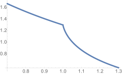
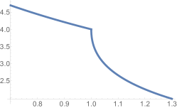
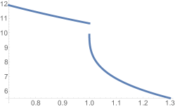
Figure 13: Plots of the limiting height function showing the formation of a traffic jam. Left: $\theta<\theta_{\mathsf{cr}}$, Center: $\theta=\theta_{\mathsf{cr}}$, Right: $\theta>\theta_{\mathsf{cr}}$.

The fluctuations of the random height function $\mathcal{H}(t,\chi)$ around the traffic jam for every fixed $\chi$ on both sides of $\boldsymbol{\upchi}$ are governed by the Airy kernel as in the first part of Theorem 4.6. However, the normalizing factor $\mathfrak{w}^{\circ}(\theta,\chi)\mathfrak{d}_{TW}(\theta,\chi)$ has a jump discontinuity at $\chi=\boldsymbol{\upchi}$.

To further explore behavior of fluctuations around a traffic jam, we consider a more general regime when $\chi=\chi(L)>\boldsymbol{\upchi}$ depends on $L$ and converges to $\boldsymbol{\upchi}$ as $L\to+\infty$. To simplify notation and computations let us take a particular case of a piecewise constant speed function

$$\xi(u)=\begin{cases}1,&0\leq u\leq 1;\\ 1/2,&u>1.\end{cases}$$ (4.14)

The critical time corresponding to formation of the traffic jam at $\boldsymbol{\upchi}=1$ is $\theta_{\mathsf{cr}}=12$, see (4.13). We find that there is a particular scale at which the fluctuations of the height function are governed by a deformation of the Tracy-Widom distribution (defined in Section C.3). This deformation can be obtained in a limit from kernels considered in [BP08] and thus has a random matrix interpretation (see Section 5.5.4 for details). At other scales the fluctuations lead to the usual Airy kernel, but close to the slowdown the constants are affected by the change in $\xi(\cdot)$ as well. Far from the slowdown the constants are the same as in (4.10) with $\chi$ depending on $L$. In detail, we show the following:

Theorem 4.7.

With the above notation, let $\chi=\chi(L)=1+10\upepsilon(L)$, where $\upepsilon(L)>0$ and $\upepsilon(L)\to 0$ as $L\to+\infty$ (the factor $10$ makes final formulas simpler). Let $\mathfrak{w}^{\circ}=\mathfrak{w}^{\circ}(12,1+10\upepsilon(L))$, $\mathfrak{h}=\mathfrak{h}(12,1+10\upepsilon(L))$, $\mathfrak{d}_{TW}=\mathfrak{d}_{TW}(12,1+10\upepsilon(L))$ be the quantities defined in Sections 4.1 and 4.3. Fix $s_{1},\ldots,s_{\ell},r_{1},\ldots,r_{\ell}\in\mathbb{R}$. Depending on the rate at which $\upepsilon(L)\to 0$ there are three fluctuation regimes:

1. (close to the slowdown) Let $\upepsilon(L)\ll L^{-4/3-\gamma}$ for some $\gamma>0$. Define

   $$t_{i}=12L+\mathfrak{w}^{\circ}\mathfrak{d}_{TW}^{2}2^{-1/3}s_{i}L^{2/3}.$$

   Then

   $$\lim_{L\to+\infty}\mathop{\mathrm{Prob}}\left(\frac{\mathcal{H}(t_{i},1+10\upepsilon(L))-4L-(\mathfrak{w}^{\circ})^{2}\mathfrak{d}_{TW}^{2}2^{-1/3}s_{i}L^{2/3}}{\mathfrak{w}^{\circ}\mathfrak{d}_{TW}2^{-2/3}L^{1/3}}>s_{i}^{2}-r_{i},\ i=1,\ldots,\ell\right)\\ =\det(\mathbf{1}-\mathsf{A}^{\mathrm{ext}})_{\sqcup_{i=1}^{\ell}\left\{s_{i}\right\}\times(r_{i},+\infty)}.$$

2. (far from the slowdown) Let $\upepsilon(L)\gg L^{-4/3+\gamma}$ for some $\gamma\in(0,\frac{4}{3})$. Define

   $$t_{i}=12L+2\mathfrak{w}^{\circ}\mathfrak{d}_{TW}^{2}s_{i}L^{2/3}.$$

   Then

   $$\lim_{L\to+\infty}\mathop{\mathrm{Prob}}\left(\frac{\mathcal{H}(t_{i},1+10\upepsilon(L))-\mathfrak{h}(12,1+10\upepsilon(L))L-2(\mathfrak{w}^{\circ})^{2}\mathfrak{d}_{TW}^{2}s_{i}L^{2/3}}{\mathfrak{w}^{\circ}\mathfrak{d}_{TW}L^{1/3}}>s_{i}^{2}-r_{i},\ i=1,\ldots,\ell\right)\\ =\det(\mathbf{1}-\mathsf{A}^{\mathrm{ext}})_{\sqcup_{i=1}^{\ell}\left\{s_{i}\right\}\times(r_{i},+\infty)}.$$

3. (critical scale) Let $\upepsilon(L)=10^{-4/3}\delta L^{-4/3}$, where $\delta>0$ is fixed. Define

   $$t_{i}=12L+\mathfrak{w}^{\circ}\mathfrak{d}_{TW}^{2}2^{-1/3}s_{i}L^{2/3}.$$

   The joint fluctuations at different times of the random height function around the limit shape $4L$ are described by a deformation of the extended Airy kernel defined by (C.6):

   $$\lim_{L\to+\infty}\mathop{\mathrm{Prob}}\left(\frac{\mathcal{H}(t_{i},1+10^{-1/3}\delta L^{-4/3})-4L-(\mathfrak{w}^{\circ})^{2}\mathfrak{d}_{TW}^{2}2^{-1/3}s_{i}L^{2/3}}{\mathfrak{w}^{\circ}\mathfrak{d}_{TW}2^{-2/3}L^{1/3}}>s_{i}^{2}+2s_{i}\delta^{1/4}-r_{i},\ i=1,\ldots,\ell\right)\\ =\det(\mathbf{1}-\widetilde{\mathsf{A}}^{\mathrm{ext},\delta})_{\sqcup_{i=1}^{\ell}\left\{s_{i}\right\}\times(r_{i},+\infty)}.$$

   In particular, for $\ell=1$ and $s_{1}=0$ we have the convergence to a deformation of the GUE Tracy-Widom distribution (C.7):

   $$\lim_{L\to+\infty}\mathop{\mathrm{Prob}}\left(\frac{\mathcal{H}(12L,1+10^{-1/3}\delta L^{-4/3})-4L}{\mathfrak{w}^{\circ}\mathfrak{d}_{TW}2^{-2/3}L^{1/3}}>-r\right)=F_{GUE}^{(\delta,0)}(r),\qquad r\in\mathbb{R}.$$

We prove Theorem 4.7 in Section 5.5.

5 Asymptotics of continuous space TASEP. Proofs

5.1 Critical points

Recall the notation (4.7):

$$G(v)=G(v;\theta,\chi,h)=-\theta v+h\log v+\displaystyle\int_{0}^{\chi}\frac{\xi(u)du}{\xi(u)-v}.$$

The correlation kernel from Theorem 3.6 takes the form

$$\mathcal{K}(t,x;t^{\prime},x^{\prime})=-\mathbf{1}_{t>t^{\prime}}\mathbf{1}_{x\geq x^{\prime}}\frac{(t-t^{\prime})^{x-x^{\prime}}}{(x-x^{\prime})!}$$

$$\hskip 30.0pt+\frac{1}{(2\pi{\mathbf{i}\mkern 1.0mu})^{2}}\oint\oint\frac{dwdz}{z(z-w)}\exp\left\{L\bigl{(}G(w;\tfrac{t^{\prime}}{L},\chi,\tfrac{x^{\prime}}{L})-G(z;\tfrac{t}{L},\chi,\tfrac{x}{L})\bigr{)}\right\}$$ (5.1)

$$\hskip 190.0pt\times\frac{(\xi(0)-z)}{(\xi(0)-w)}\prod\limits_{b\in\mathbf{B}\colon b<\chi}\frac{\xi(b)-p(b)w}{\xi(b)-p(b)z}\cdot\frac{\xi(b)-z}{\xi(b)-w},$$

where we used the observation $\int_{0}^{\chi}\frac{\xi(u)du}{\xi(u)-v}=\chi+\int_{0}^{\chi}\frac{v\,du}{\xi(u)-v}$, and the additional summand $\chi$ cancels out in $G(w)-G(z)$. The integration contours in (5.1) are described in Theorem 3.6.

The asymptotic behavior of the kernel as $\mathcal{K}$ as $L\to+\infty$ is analyzed via steepest descent method which in turn relies on finding double critical points of the function $G$, i.e., those $v$ for which $\frac{\partial}{\partial v}G(v)=\frac{\partial^{2}}{\partial v^{2}}G(v)=0$ and $\frac{\partial^{3}}{\partial v^{3}}G(v)\neq 0$. We turn to double critical points because we are interested in the left edge of the determinantal point process $\widetilde{\mathfrak{L}}_{\ell}$. The equations for the double critical points of $G(v;\theta,\chi,h)$ can be rewritten the following form:

$$\int_{0}^{\chi}\frac{\xi(u)(v+\xi(u))}{\left(\xi(u)-v\right)^{3}}\,du=\theta;$$ (5.2)

$$h=\theta v-\int_{0}^{\chi}\frac{\xi(u)v}{\left(\xi(u)-v\right)^{2}}\,du.$$ (5.3)

Recall that $\mathcal{W}^{\circ}_{\chi}$ is the essential minimum of the function $\xi(u)$ for $0<u<\chi$, and $\mathcal{W}_{\chi}$ is the minimum of $\mathcal{W}^{\circ}_{\chi}$, $\xi(0)$, and values of $\xi$ at all the roadblocks on $(0,\chi)$, see (4.2)–(4.3). By Lemma 4.2, for $(\theta,\chi)$ in the curved part (Definition 4.1) the first equation (5.2) has a unique solution (denoted by $\mathfrak{w}^{\circ}=\mathfrak{w}^{\circ}(\theta,\chi)$) in $v$ belonging to $(0,\mathcal{W}^{\circ}_{\chi})$.

Recall the notation $\mathfrak{w}(\theta,\chi)=\min(\mathfrak{w}^{\circ}(\theta,\chi),\mathcal{W}_{\chi})$ and limit shape $\mathfrak{h}(\theta,\chi)$ from Definition 4.3. In the Tracy-Widom phase the limit shape $\mathfrak{h}(\theta,\chi)$ is defined by plugging $\mathfrak{w}^{\circ}(\theta,\chi)$ into the second double critical point equation (5.3), so that $\mathfrak{w}(\theta,\chi)=\mathfrak{w}^{\circ}(\theta,\chi)$ is a double critical point of $G(v;\theta,\chi,\mathfrak{h}(\theta,\chi))$. In the Gaussian phase and at the BBP transition, $\mathfrak{w}(\theta,\chi)=\mathcal{W}_{\chi}$ is a single critical point of $G(v;\theta,\chi,\mathfrak{h}(\theta,\chi))$.

5.2 Estimates on contours

Here we prove estimates of the real part of the function $G(v;\theta,\chi,\mathfrak{h}(\theta,\chi))$ on the following contours:

Definition 5.1.

For $r>0$ let $\Gamma_{r}$ be the counterclockwise circle centered at zero and passing through $r$. Let $C_{r,\varphi}$ (where $0<\varphi<\pi/2$) be the contour

$$C_{r,\varphi}:=\{r-{\mathbf{i}\mkern 1.0mu}ye^{{\mathbf{i}\mkern 1.0mu}\varphi\mathop{\mathrm{sgn}}(y)}\colon y\in\mathbb{R}\}$$

composed of two lines passing through $r$ which form angle $\varphi$ with the vertical axis. In this section we mostly need the contour $C_{r,\frac{\pi}{4}}$ which will be denoted simply by $C_{r}$. See Figure 14 for an illustration.

Figure 14: Contours $\Gamma_{r}$ and $C_{r}=C_{r,\frac{\pi}{4}}$.

We need slightly different arguments depending on the phase (Definition 4.4). We start from the Tracy-Widom one.

Lemma 5.2.

Let $(\theta,\chi)$ be in the Tracy-Widom phase. The contour $\Gamma_{\mathfrak{w}^{\circ}(\theta,\chi)}$ is steep ascent for the function $\mathop{\mathrm{Re}}G(z;\theta,\chi,\mathfrak{h}(\theta,\chi))$ in the sense that the function attains its minimal value at $z=\mathfrak{w}^{\circ}(\theta,\chi)$.

Proof.

For shorter notation we denote $\mathfrak{h}=\mathfrak{h}(\theta,\chi)$ and $\mathfrak{w}=\mathfrak{w}^{\circ}(\theta,\chi)$ in the proof of this lemma and Lemma 5.3 below.

From (5.2)–(5.3) we can write

$$G(z;\theta,\chi,\mathfrak{h})=\int_{0}^{\chi}S(z;\xi(u))du,$$

where

$$S(z)=S(z;\xi(u)):=\log z\left(\frac{\xi(u)(\xi(u)+\mathfrak{w})\mathfrak{w}}{(\xi(u)-\mathfrak{w})^{3}}-\frac{\xi(u)\mathfrak{w}}{(\xi-\mathfrak{w})^{2}}\right)-\frac{z\xi(u)(\xi(u)+\mathfrak{w})}{(\xi(u)-\mathfrak{w})^{3}}+\frac{\xi(u)}{\xi(u)-z}.$$

Denote $\gamma(u)=\xi(u)-\mathfrak{w}.$ We know that $\xi(u)\geq\mathfrak{w},$ thus, $\gamma(u)$ is nonnegative. We get

$$S(z;\xi(u))=(\mathfrak{w}+\gamma(u))\left(\frac{1}{\mathfrak{w}+\gamma(u)-z}-\frac{z(2\mathfrak{w}+\gamma(u))}{\gamma(u)^{3}}+\frac{2\mathfrak{w}^{2}\log z}{\gamma(u)^{3}}\right).$$ (5.4)

Let us prove $\frac{\partial}{\partial\varphi}\mathop{\mathrm{Re}}S(\mathfrak{w}e^{{\mathbf{i}\mkern 1.0mu}\varphi})>0$ for $0<\varphi<\pi$. The case $-\pi<\varphi<0$ is symmetric. Straightforward computation gives (we are omitting the dependence on $u$ in the notation)

$$\frac{\partial}{\partial\varphi}\mathop{\mathrm{Re}}S(\mathfrak{w}e^{{\mathbf{i}\mkern 1.0mu}\varphi})=\frac{16\mathfrak{w}^{2}(\gamma+\mathfrak{w})^{2}(\gamma+2\mathfrak{w})\sin^{3}\left(\frac{\varphi}{2}\right)\cos\left(\frac{\varphi}{2}\right)\left(\gamma^{2}+\mathfrak{w}^{2}(1-\cos\varphi)+\gamma\mathfrak{w}(1-\cos\varphi)\right)}{\gamma^{3}\left(\gamma^{2}+2\mathfrak{w}^{2}+2\gamma\mathfrak{w}-2\mathfrak{w}(\gamma+\mathfrak{w})\cos\varphi\right)^{2}}.$$ (5.5)

We see that for $\pi>\varphi\geq 0$ this quantity is positive, which implies the statement. ∎

Lemma 5.3.

Let $(\theta,\chi)$ be in the Tracy-Widom phase. The contour $C_{\mathfrak{w}^{\circ}(\theta,\chi)}$ is steep descent for the function $\mathop{\mathrm{Re}}G(w;\theta,\chi,\mathfrak{h}(\theta,\chi))$ in the sense that the function attains its maximal value at $w=\mathfrak{w}^{\circ}(\theta,\chi)$.

Proof.

Using the notation from the proof of Lemma 5.2 we will show that $\frac{\partial}{\partial s}\mathop{\mathrm{Re}}S(\mathfrak{w}+se^{{\mathbf{i}\mkern 1.0mu}\frac{\pi}{4}})<0$ for $s>0$ (the case $s<0$ and $-\frac{\pi}{4}$ is symmetric). This would imply the statement of the proposition. A straightforward computation gives that this derivative is (up to an obviously positive denominator) equal to

$$\begin{split}&-s^{2}(\mathfrak{w}+\gamma)\bigl{(}\gamma(\sqrt{2}s^{2}-4s\gamma+3\sqrt{2}\gamma^{2})(s^{2}+\mathfrak{w}^{2})+2Q(s,\gamma)\mathfrak{w}\bigr{)},\quad\text{where}\\ &\hskip 180.0ptQ(s,\gamma)=\sqrt{2}s^{4}-3s^{3}\gamma+2\sqrt{2}s^{2}\gamma^{2}-s\gamma^{3}+\sqrt{2}\gamma^{4}\end{split}$$

(here we omitted the dependence on $u$). The discriminant of $\sqrt{2}s^{2}-4s\gamma+3\sqrt{2}\gamma^{2}$ in $s$ is $-8\gamma^{2},$ so this expression is positive. The discriminant of $Q(s,\gamma)$ in $\gamma$ is $1684s^{12}>0,$ so $Q(s,\gamma)$ either has all real or all nonreal complex roots in $\gamma$. Note that

$$\frac{\partial}{\partial\gamma}Q(s,\gamma)=(4\sqrt{2}\gamma-3s)(s^{2}+\gamma^{2}),$$

which has only one root in $\gamma$. Therefore, $Q(s,\gamma)$ has only nonreal roots and thus preserves sign. It is always positive because it is positive for $\gamma=0$. This shows that $\frac{\partial}{\partial s}\mathop{\mathrm{Re}}S$ is negative, which implies the claim. ∎

Let us now turn to the Gaussian phase.

Lemma 5.4.

Let $(\theta,\chi)$ be in the Gaussian phase or at a BBP transition. The contour $\Gamma_{\mathcal{W}_{\chi}}$ is steep ascent for the function $\mathop{\mathrm{Re}}G(z;\theta,\chi,\mathfrak{h}(\theta,\chi))$ in the sense that the function attains its minimal value at $z=\mathcal{W}_{\chi}$.

Proof.

Throughout the proof (and in the proof of Lemma 5.5 below) we use the shorthand notation $\mathfrak{w}^{\circ}=\mathfrak{w}^{\circ}(\theta,\chi)$ and $\mathcal{W}=\mathcal{W}_{\chi}$.

Let us write $G(z;\theta,\chi,\mathfrak{h}(\theta,\chi))$ again as an integral from $0$ to $\chi$. While $\mathfrak{h}$ depends on $\mathcal{W}$ (Definition 4.3), we cannot express $\theta$ through $\mathcal{W}$. However, we can still write $\theta$ in terms of the solution $\mathfrak{w}^{\circ}(\theta,\chi)\geq\mathcal{W}_{\chi}$ to equation (5.2). This allows to write

$$G(z;\theta,\chi,\mathfrak{h}(\theta,\chi))=\int_{0}^{\chi}\tilde{S}(z;\xi(u))du,$$

where

$$\tilde{S}(z;\xi):=-\log z\,\frac{\xi\mathcal{W}}{(\xi-\mathcal{W})^{2}}+\frac{\xi}{\xi-z}+(\mathcal{W}\log z-z)\frac{\xi(\xi+\mathfrak{w}^{\circ})}{(\xi-\mathfrak{w}^{\circ})^{3}}.$$

We estimate for $0\leq\varphi<\pi$ (the case $-\pi<\varphi<0$ is symmetric)

$$\frac{\partial}{\partial\varphi}\mathop{\mathrm{Re}}\tilde{S}(\mathcal{W}e^{{\mathbf{i}\mkern 1.0mu}\varphi},\xi) =\frac{\mathcal{W}\xi\left(\mathcal{W}^{2}-\xi^{2}\right)\sin\varphi}{\left(\mathcal{W}^{2}-2\mathcal{W}\xi\cos\varphi+\xi^{2}\right)^{2}}+\frac{\mathcal{W}\xi(\mathfrak{w}^{\circ}+\xi)\sin\varphi}{(\xi-\mathfrak{w}^{\circ})^{3}}$$

$$\geq\frac{\mathcal{W}\xi\left(\mathcal{W}^{2}-\xi^{2}\right)\sin\varphi}{\left(\mathcal{W}^{2}-2\mathcal{W}\xi\cos\varphi+\xi^{2}\right)^{2}}+\frac{\mathcal{W}\xi(\mathcal{W}+\xi)\sin\varphi}{(\xi-\mathcal{W})^{3}},$$

where we used $\mathcal{W}\xi\sin\varphi\geq 0$, $\mathfrak{w}^{\circ}\geq\mathcal{W}$, and that the function $u\mapsto\frac{\xi+u}{(\xi-u)^{3}}$ is increasing for $0<u<\xi$. The right-hand side coincides with (5.5) with $\mathfrak{w}$ replaced by $\mathcal{W}$, and thus is positive as shown in the proof of Lemma 5.2. Therefore, $\frac{\partial}{\partial\varphi}\mathop{\mathrm{Re}}\tilde{S}(\mathcal{W}e^{{\mathbf{i}\mkern 1.0mu}\varphi},\xi)>0$ for $0<\varphi<\pi$, and we are done. ∎

Lemma 5.5.

Let $(\theta,\chi)$ be in the Gaussian phase or at a BBP transition. The contour $C_{\mathcal{W}_{\chi}}$ is steep descent for the function $\mathop{\mathrm{Re}}G(w;\theta,\chi,\mathfrak{h}(\theta,\chi))$ in the sense that the function attains its maximal value at $w=\mathcal{W}_{\chi}$.

Proof.

Using the notation from the proof of Lemma 5.4 let us show that $\frac{\partial}{\partial s}\tilde{S}(\mathcal{W}+se^{{\mathbf{i}\mkern 1.0mu}\frac{\pi}{4}},\xi)<0$ for $s<0$ (the case of the line at angle $-\frac{\pi}{4}$ in the lower half plane is symmetric). This derivative is equal to

$$-\frac{\xi\mathcal{W}\left(2s+\sqrt{2}\mathcal{W}\right)}{2\left(s^{2}+\sqrt{2}s\mathcal{W}+\mathcal{W}^{2}\right)(\mathcal{W}-\xi)^{2}}+\frac{\xi\left(\sqrt{2}s^{2}+4s(\mathcal{W}-\xi)+\sqrt{2}(\mathcal{W}-\xi)^{2}\right)}{2\left(s^{2}+\sqrt{2}s(\mathcal{W}-\xi)+(\mathcal{W}-\xi)^{2}\right)^{2}}\\ -\frac{\xi s^{2}(\mathfrak{w}^{\circ}+\xi)}{\sqrt{2}(\xi-\mathfrak{w}^{\circ})^{3}\left(s^{2}+\sqrt{2}s\mathcal{W}+\mathcal{W}^{2}\right)}.$$

Again, in the last summand we can replace $\mathfrak{w}^{\circ}$ by $\mathcal{W}$ by the monotonicity of $u\mapsto\frac{\xi+u}{(\xi-u)^{3}}$ as in the previous lemma, and the whole expression may only decrease. Then we use the proof of Lemma 5.3 which implies that $\frac{\partial}{\partial s}\tilde{S}(\mathcal{W}+se^{{\mathbf{i}\mkern 1.0mu}\frac{\pi}{4}},\xi)<0$, as desired. ∎

We need two more statements about higher derivatives of the function $G$.

Lemma 5.6.

Let $(\theta,\chi)$ be in the curved part. We have

$$\frac{\partial^{3}}{\partial^{3}v}\Big{|}_{v=\mathfrak{w}(\theta,\chi)}G(v;\theta,\chi,\mathfrak{h}(\theta,\chi))>0.$$

Proof.

We have $G^{(3)}(\mathfrak{w})=\frac{2\mathfrak{h}}{\mathfrak{w}^{3}}+\int_{0}^{\chi}\frac{6\xi(u)du}{(\xi(u)-\mathfrak{w})^{4}}>0$, as desired. ∎

Lemma 5.7.

Let $(\theta,\chi)$ be in the curved part. Along the contour $\Gamma_{\mathfrak{w}(\theta,\chi)}$ the first $m$ derivatives of $\mathop{\mathrm{Re}}G(z;\theta,\chi,\mathfrak{h}(\theta,\chi))$ at $\mathfrak{w}(\theta,\chi)$ vanish while the $(m+1)$-st one is nonzero, where $m=3$ in the Tracy-Widom phase and at a BBP transition, and $m=1$ in the Gaussian phase. Along the contour $C_{\mathfrak{w}(\theta,\chi)}$ the first two derivatives of $\mathop{\mathrm{Re}}G(z;\theta,\chi,\mathfrak{h}(\theta,\chi))$ at $\mathfrak{w}(\theta,\chi)$ vanish while the third one is nonzero.

Proof.

This is checked in a straightforward way. ∎

5.3 Deformation of contours and behavior of the kernel

Assume that $(\theta,\chi)$ is in the curved part and we scale $t,t^{\prime}=\theta L+o(L)$, $x,x^{\prime}=\mathfrak{h}(\theta,\chi)L+o(L)$ (more precise scaling depends on the phase and is described below in this subsection). Let us deform the $z$ and $w$ integration contours in the correlation kernel (5.1) to the steep ascent/descent contours $\Gamma_{\mathfrak{w}(\theta,\chi)}$ and $C_{\mathfrak{w}(\theta,\chi)}$, respectively.

Since $\mathfrak{w}(\theta,\chi)\leq\mathcal{W}_{\chi}=\min\Xi_{\chi}$, see (4.2), the $z$ contour can be deformed to $\Gamma_{\mathfrak{w}(\theta,\chi)}$ without passing through any singularities.

To deform the $w$ contour we need to open it up to infinity. Fix sufficiently large $L$. Since $(\theta,\chi)$ is in the curved part, we have $\theta,\chi>0$. Then the terms $-L\theta w-L\int_{0}^{\chi}\frac{\xi(u)du}{w-\xi(u)}$ in the exponent in the integrand have large negative real part for $\mathop{\mathrm{Re}}w\gg 1$, and thus dominate the behavior of the integrand for large $|w|$ if $w$ is in the right half plane. Therefore, we can deform the $w$ contour to the desired one. (In the Gaussian phase or at a BBP transition we require, in addition, that locally $w$ passes strictly to the right of the pole at $w=\mathcal{W}_{\chi}$.)

We can now obtain the asymptotic behavior of the correlation kernel $\mathcal{K}$ (5.1) close to the left edge of the determinantal point process $\widetilde{\mathfrak{L}}_{\ell}$. Recall the quantity $\mathfrak{d}_{TW}=\mathfrak{d}_{TW}(\theta,\chi)>0$ (4.8).

Proposition 5.8 (Kernel asymptotics, Tracy-Widom phase).

Let $(\theta,\chi)$ be in the Tracy-Widom phase and scale the parameters as

$$\begin{split}t=\theta L+2\mathfrak{w}^{\circ}\mathfrak{d}_{TW}^{2}s^{\prime}L^{2/3},\qquad x&=\lfloor\mathfrak{h}L+2(\mathfrak{w}^{\circ})^{2}\mathfrak{d}_{TW}^{2}s^{\prime}L^{2/3}+\mathfrak{w}^{\circ}\mathfrak{d}_{TW}(s^{\prime 2}-h^{\prime})L^{1/3}\rfloor,\\ t^{\prime}=\theta L+2\mathfrak{w}^{\circ}\mathfrak{d}_{TW}^{2}sL^{2/3},\qquad x^{\prime}&=\lfloor\mathfrak{h}L+2(\mathfrak{w}^{\circ})^{2}\mathfrak{d}_{TW}^{2}sL^{2/3}+\mathfrak{w}^{\circ}\mathfrak{d}_{TW}(s^{2}-h)L^{1/3}\rfloor,\end{split}$$ (5.6)

where $s,s^{\prime},h,h^{\prime}\in\mathbb{R}$ are arbitrary. Then as $L\to+\infty$ we have

$$\mathcal{K}(t,x;t^{\prime},x^{\prime})=e^{f_{2}L^{2/3}+f_{1}L^{1/3}}\,\frac{1+O(L^{-1/3})}{L^{1/3}\mathfrak{d}_{TW}\mathfrak{w}^{\circ}}\,\widetilde{\mathsf{A}}^{\mathrm{ext}}(s,h;s^{\prime},h^{\prime}),$$ (5.7)

where the constant in $O(L^{-1/3})$ is uniform in $h,h^{\prime}$ belonging to compact intervals, but may depend on $s,s^{\prime}$. Here $\widetilde{\mathsf{A}}^{\mathrm{ext}}$ is (a version of) the extended Airy₂ kernel (C.2), and

$$\begin{split}f_{1}&:=(h^{\prime}-h+s^{2}-s^{\prime 2})\mathfrak{d}_{TW}\mathfrak{w}^{\circ}\log\mathfrak{w}^{\circ},\\ f_{2}&:=2(s^{\prime}-s)\mathfrak{d}_{TW}^{2}(\mathfrak{w}^{\circ})^{2}(1-\log\mathfrak{w}^{\circ}).\end{split}$$ (5.8)

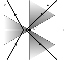
Figure 15: Local behavior of the integration contours in a neighborhood of the double critical point $\mathfrak{w}^{\circ}$. The regions where $\mathop{\mathrm{Re}}(\tilde{w}^{3})<0$ are shaded.

Remark 5.9.

1. Here and below in scalings like (5.6) we essentially transpose the pre-limit kernel by assigning the primed scaled variables $s^{\prime},h^{\prime}$ to the non-primed $t,x$. This transposition is needed so that (5.7) holds without switching $(s,h)\leftrightarrow(s^{\prime},h^{\prime})$. Transposing a correlation kernel does not change the determinantal point process and thus does not affect our asymptotic results.

2. The factor $e^{f_{2}L^{2/3}+f_{1}L^{1/3}}$ is a gauge transformation of a determinantal correlation kernel which in general looks as $K(x,y)\mapsto\frac{f(x)}{f(y)}K(x,y)$ (with nonvanishing $f$). Gauge transformations do not change determinants associated with the kernel.

Proof of Proposition 5.8.

One can readily check that $\mathfrak{d}_{TW}=\sqrt[3]{\frac{1}{2}G^{(3)}(\mathfrak{w}^{\circ})}$. Deform the integration contours as explained in the beginning of the subsection in the kernel (5.1) so that they are $\Gamma_{\mathfrak{w}^{\circ}}$ and $C_{\mathfrak{w}^{\circ}}$, respectively, and change the variables in a neighborhood of size $L^{-1/6+\varepsilon}$ (where $\varepsilon>0$ is small and fixed) of the double critical point $\mathfrak{w}^{\circ}$ as

$$z=\mathfrak{w}^{\circ}+\frac{\tilde{z}}{\mathfrak{d}_{TW}L^{1/3}},\qquad w=\mathfrak{w}^{\circ}+\frac{\tilde{w}}{\mathfrak{d}_{TW}L^{1/3}},$$ (5.9)

where $\tilde{z},\tilde{w}$ belong to the contours given in Figure 15 and are bounded in absolute value by $L^{1/6+\varepsilon}$. The exponent in the kernel behaves as

$$\begin{split}&L\bigl{(}G(w;\tfrac{t^{\prime}}{L},\chi,\tfrac{x^{\prime}}{L})-G(z;\tfrac{t}{L},\chi,\tfrac{x}{L})\bigr{)}=L\bigl{(}G(w;\theta,\chi,\mathfrak{h}(\theta,\chi))-G(z;\theta,\chi,\mathfrak{h}(\theta,\chi))\bigr{)}\\ &\hskip 140.0pt-(t^{\prime}-\theta L)w+(t-\theta L)z+(x^{\prime}-\mathfrak{h}L)\log w-(x-\mathfrak{h}L)\log z\\ &\hskip 15.0pt=L^{2/3}f_{2}+L^{1/3}f_{1}+\tfrac{1}{3}\tilde{w}^{3}-s\tilde{w}^{2}-(h-s^{2})\tilde{w}-\tfrac{1}{3}\tilde{z}^{3}+s^{\prime}\tilde{z}^{2}+(h^{\prime}-s^{\prime 2})\tilde{z}+o(1),\end{split}$$ (5.10)

where $f_{1},f_{2}$ are given by (5.8). The remaining factors in the integrand are

$$\frac{dwdz}{z(z-w)}=-\frac{d\tilde{w}d\tilde{z}}{L^{1/3}\mathfrak{w}^{\circ}\mathfrak{d}_{TW}(\tilde{w}-\tilde{z})}\,\bigl{(}1+o(1)\bigr{)}$$ (5.11)

(the negative sign in the right-hand side is absorbed by reversing one of the contours in Figure 15), and

$$\frac{(\xi(0)-z)}{(\xi(0)-w)}\prod\limits_{b\in\mathbf{B}\colon b<\chi}\frac{\xi(b)-p(b)w}{\xi(b)-p(b)z}\cdot\frac{\xi(b)-z}{\xi(b)-w}=1+o(1).$$ (5.12)

Next, with the help of the Stirling asymptotics for the Gamma function (cf. [Erd53, 1.18.(1)]) one readily sees that the additional summand in (5.1) behaves as

$$-\mathbf{1}_{t>t^{\prime},\,x\geq x^{\prime}}\frac{(t-t^{\prime})^{x-x^{\prime}}}{(x-x^{\prime})!}=-\mathbf{1}_{s^{\prime}>s}\,e^{f_{2}L^{2/3}+f_{1}L^{1/3}}\frac{\exp\left\{-\frac{(h-h^{\prime}-s^{2}+s^{\prime 2})^{2}}{4(s^{\prime}-s)}\right\}}{L^{1/3}\mathfrak{d}_{TW}\mathfrak{w}^{\circ}\sqrt{4\pi(s^{\prime}-s)}}\,(1+O(L^{-1/3})).$$ (5.13)

We thus get $e^{-f_{2}L^{2/3}-f_{1}L^{1/3}}\mathcal{K}(t,x;t^{\prime},x^{\prime})\approx(L^{1/3}\mathfrak{d}_{TW}\mathfrak{w}^{\circ})^{-1}\widetilde{\mathsf{A}}^{\mathrm{ext}}(s,h;s^{\prime},h^{\prime})$, as desired.

It remains to show that the behavior of the double contour integral coming from the neighborhood of size $L^{-1/6+\varepsilon}$ of the double critical point $\mathfrak{w}^{\circ}$ indeed determines the asymptotics of the kernel, and show the uniformity of the constant in the error $O(L^{-1/3})$ in (5.7).

First, note that both $\mathfrak{w}^{\circ}(\theta,\chi)$ and $\mathfrak{d}_{TW}(\theta,\chi)$ are uniformly bounded away from $0$ for $(\theta,\chi)$ in a compact subset of the curved part. One can check that in (5.13) the constant by the error $L^{-1/3}$ contains powers of $\mathfrak{w}^{\circ}$, $\mathfrak{d}_{TW}$, and $s^{\prime}-s$ in the denominator, and thus the error is uniform in $\theta,\chi,h,h^{\prime}$ in compact sets.

Let us now turn to the double contour integral, and first consider the case when $z,w$ are inside the $L^{-1/6+\varepsilon}$-neighborhood of $\mathfrak{w}^{\circ}$. Note that the contours $\tilde{z},\tilde{w}$ are separated from each other. The $o(1)$ errors coming from (5.10), (5.11), and (5.12) combined produce in front of the exponent a function bounded in absolute value by a polynomial in $\tilde{z},\tilde{w}$ times $\mathrm{const}\cdot L^{-1/3}$. The Airy-type double contour integral with such additional polynomial factors converges, so we get a uniform error of order $L^{-1/3}$. Therefore, the double contour integral in (5.1) with $z,w$ in the $L^{-1/6+\varepsilon}$-neighborhood of $\mathfrak{w}^{\circ}$ is equal to $1+O(L^{-1/3})$ times the double contour integral in (C.2) with $|u|,|v|<L^{1/6+\varepsilon}$. The double contour integral over the remaining parts of the contours can be bounded by $e^{-cL^{1/2+3\varepsilon}}$ and is thus negligible. Thus, we get the desired contribution from the small neighborhood of $\mathfrak{w}^{\circ}$.

Next, write for the real part similarly to (5.10):

$$\begin{split}&L\mathop{\mathrm{Re}}\bigl{(}G(w;\tfrac{t^{\prime}}{L},\chi,\tfrac{x^{\prime}}{L})-G(z;\tfrac{t}{L},\chi,\tfrac{x}{L})\bigr{)}=L\mathop{\mathrm{Re}}\bigl{(}G(w;\theta,\chi,\mathfrak{h}(\theta,\chi))-G(z;\theta,\chi,\mathfrak{h}(\theta,\chi))\bigr{)}\\ &\hskip 90.0pt-(t^{\prime}-\theta L)\mathop{\mathrm{Re}}w+(t-\theta L)\mathop{\mathrm{Re}}z+(x^{\prime}-\mathfrak{h}L)\log|w|-(x-\mathfrak{h}L)\log\mathfrak{w}^{\circ}.\end{split}$$ (5.14)

By Lemmas 5.2, 5.3 and 5.7 there exists $\delta>0$ such that if $z$ or $w$ or both are outside the $\delta$-neighborhood of $\mathfrak{w}^{\circ}$, the above quantity is bounded from above by $-cL$ for some $c>0$. Indeed, this bound is valid for the first line in (5.14) while the terms in the second line as well as the gauge factor $-f_{2}L^{2/3}-f_{1}L^{1/3}$ are of smaller order.

It remains to consider the case when both $z,w$ are inside the $\delta$-neighborhood of $\mathfrak{w}^{\circ}$ but at least one is outise the $L^{-1/6+\varepsilon}$-neighborhood. Let use the notation $w=\mathfrak{w}^{\circ}+r(1+{\mathbf{i}\mkern 1.0mu})$, $z=\mathfrak{w}^{\circ}e^{{\mathbf{i}\mkern 1.0mu}\varphi}$ where we can assume (by shrinking or enlarging the $\delta$-neighborhood by a constant factor) that $0<r<\delta$, $0<\varphi<\delta$, $\max(r,\varphi)>L^{-1/6+\varepsilon}$. For the first line in the right-hand side of (5.14) we can write by Lemma 5.7:

$$L\mathop{\mathrm{Re}}\bigl{(}G(w;\theta,\chi,\mathfrak{h}(\theta,\chi))-G(z;\theta,\chi,\mathfrak{h}(\theta,\chi))\bigr{)}\leq-cL(r^{3}+\varphi^{4}).$$ (5.15)

Adding the terms $-f_{2}L^{2/3}-f_{1}L^{1/3}$ to the second line we can estimate its absolute value as

$$\Bigl{|}-f_{2}L^{2/3}-f_{1}L^{1/3}-(t^{\prime}-\theta L)\mathop{\mathrm{Re}}w+(t-\theta L)\mathop{\mathrm{Re}}z+(x^{\prime}-\mathfrak{h}L)\log|w|-(x-\mathfrak{h}L)\log\mathfrak{w}^{\circ}\Bigr{|}\\ \leq c_{2}L^{2/3}(r^{3}+\varphi^{2})+c_{1}L^{1/3}r.$$

One readily sees that the terms in (5.15) dominate by at least a factor of $L^{2\varepsilon}$, and thus the contribution to the double contour integral from this remaining case is also asymptotically negligible. This completes the proof. ∎

The next two propositions deal with the BBP and the Gaussian cases. As justifications of estimates in these cases are very similar to the proof of Proposition 5.8, we omit these arguments and only present the main computations. For the next two statements recall the notation $m_{\chi}$ (4.6).

Proposition 5.10 (Kernel asymptotics, BBP transition).

Let $(\theta,\chi)$ be at a BBP transition. Scale the parameters as (5.6), where $s,s^{\prime},h,h^{\prime}\in\mathbb{R}$ are arbitrary. Then as $L\to+\infty$ for fixed $s,s^{\prime}$ we have

$$\mathcal{K}(t,x;t^{\prime},x^{\prime})=e^{f_{2}L^{2/3}+f_{1}L^{1/3}}\,\frac{1+O(L^{-1/3})}{L^{1/3}\mathfrak{d}_{TW}\mathfrak{w}^{\circ}}\,\widetilde{\mathsf{B}}^{\mathrm{ext}}_{m_{\chi},(0,\ldots,0)}(s,h;s^{\prime},h^{\prime}),$$ (5.16)

with the gauge factors (5.8) and the extended BBP kernel (C.5). The constant in $O(L^{-1/3})$ is uniform in the same way as in Proposition 5.8.

Proof.

Recall that at a BBP transition we have $\mathfrak{w}^{\circ}(\theta,\chi)=\mathcal{W}_{\chi}$. The proof is very similar to the one of Proposition 5.8. We deform the $z$ and $w$ integration contours in (5.1) so that they are $\Gamma_{\mathfrak{w}^{\circ}}$ and $C_{\mathfrak{w}^{\circ}}$, respectively, as explained in the beginning of the subsection. In particular, the pole at $w=\mathfrak{w}^{\circ}$ stays to the right of all the contours. We then make the change of variables (5.9) in a $L^{-1/6+\varepsilon}$-neighborhood of $\mathfrak{w}^{\circ}$. The scaled variables $\tilde{z},\tilde{w}$ belong to the contours given in Figure 15.

The asymptotic expansions of the exponent (5.10) and the factors (5.11) are the same at our phase transition. The behavior of the additional summand (5.13) also stays the same. The difference with the Tracy-Widom phase comes from the asymptotics of the product (5.12) which must be replaced by

$$\frac{(\xi(0)-z)}{(\xi(0)-w)}\prod\limits_{b\in\mathbf{B}\colon b<\chi}\frac{\xi(b)-p(b)w}{\xi(b)-p(b)z}\cdot\frac{\xi(b)-z}{\xi(b)-w}=(1+o(1))\prod_{b\in\mathbf{B}\colon\xi(b)=\mathfrak{w}^{\circ}}\frac{\mathfrak{w}^{\circ}-z}{\mathfrak{w}^{\circ}-w}=(1+o(1))\left(\frac{\tilde{z}}{\tilde{w}}\right)^{m_{\chi}}.$$

Combining these expansions (and omitting error estimates outside a small neighborhood of the critical point which are analogous to Proposition 5.8) one gets the claim. ∎

For the next statement recall the quantity $\mathfrak{d}_{G}(\theta,\chi)>0$ (4.9) and denote

$$\mathfrak{d}_{G}:=\mathfrak{d}_{G}(\theta,\chi),\qquad\mathfrak{d}_{G}^{\prime}:=\mathfrak{d}_{G}(\theta^{\prime},\chi),\qquad\mathfrak{h}:=\mathfrak{h}(\theta,\chi),\qquad\mathfrak{h}^{\prime}:=\mathfrak{h}(\theta^{\prime},\chi).$$

Proposition 5.11 (Kernel asymptotics, Gaussian phase).

Let $(\theta,\chi)$ and $(\theta^{\prime},\chi)$ be in the Gaussian phase, and scale the parameters as

$$\begin{split}t=\theta^{\prime}L+\mathfrak{d}_{G}^{\prime}s^{\prime}L^{1/2},\qquad x&=\lfloor\mathfrak{h}^{\prime}L+\mathfrak{d}_{G}^{\prime}\mathcal{W}(s^{\prime}-h^{\prime})L^{1/2}\rfloor,\\ t^{\prime}=\theta L+\mathfrak{d}_{G}sL^{1/2},\qquad x^{\prime}&=\lfloor\mathfrak{h}L+\mathfrak{d}_{G}\mathcal{W}(s-h)L^{1/2}\rfloor,\end{split}$$ (5.17)

where $s,s^{\prime},h,h^{\prime}\in\mathbb{R}$ are arbitrary. Then as $L\to+\infty$ we have with $\widetilde{\mathsf{G}}$ given by (C.8):

$$\mathcal{K}(t,x;t^{\prime},x^{\prime})=e^{\tilde{f}_{0}L+\tilde{f}_{1}L^{1/2}}\frac{1+O(L^{-1/2})}{L^{1/2}\mathfrak{d}_{G}\mathcal{W}_{\chi}}\,\widetilde{\mathsf{G}}^{\mathrm{ext}}_{m,\mathfrak{d}_{G}^{\prime}/\mathfrak{d}_{G}}(h;h^{\prime}),$$ (5.18)

where

$$\tilde{f}_{0}:=\mathcal{W}(\theta-\theta^{\prime})(\log\mathcal{W}-1),\qquad\tilde{f}_{1}:=\mathcal{W}\left(\mathfrak{d}_{G}^{\prime}s^{\prime}-\mathfrak{d}_{G}s+\left(\mathfrak{d}_{G}(s-h)-\mathfrak{d}_{G}^{\prime}(s^{\prime}-h^{\prime})\right)\log\mathcal{W}\right),$$ (5.19)

and the constant in $O(L^{-1/2})$ is uniform in $h,h^{\prime}$ belonging to compact intervals, but may depend on $s,s^{\prime}$.

Proof.

Recall that in the Gaussian phase we have $\mathfrak{w}^{\circ}(\theta,\chi)>\mathcal{W}_{\chi}$, and the critical point of interest is now $\mathcal{W}:=\mathcal{W}_{\chi}$ which does not depend on $\theta$. This critical point is single and not double as in the previous two statements. Deform the $z$ and $w$ contours in (5.1) to be $\Gamma_{\mathcal{W}}$ and $C_{\mathcal{W}}$, respectively. In a neighborhood of $\mathcal{W}$ of size $L^{-1/4+\varepsilon}$ (for small fixed $\varepsilon>0$) make a change of variables

$$z=\mathcal{W}+\frac{\tilde{z}}{\mathfrak{d}_{G}^{\prime}L^{1/2}},\qquad w=\mathcal{W}+\frac{\tilde{w}}{\mathfrak{d}_{G}L^{1/2}},$$

where $\tilde{z},\tilde{w}$ belong to the contours in Figure 16 and are bounded in absolute value by $L^{1/4+\varepsilon}$. One can readily check that $\mathfrak{d}_{G}=\sqrt{-G^{\prime\prime}(\mathcal{W}_{\chi};\theta,\chi,\mathfrak{h})}$, $\mathfrak{d}_{G}^{\prime}=\sqrt{-G^{\prime\prime}(\mathcal{W}_{\chi};\theta^{\prime},\chi,\mathfrak{h}^{\prime})}$.

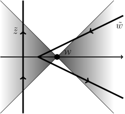
Figure 16: Local behavior of the integration contours in a neighborhood of the single critical point $\mathcal{W}$. The contour $\tilde{z}$ must lie to the left of the contour $\tilde{w}\mathfrak{d}_{G}^{\prime}/\mathfrak{d}_{G}$. Shaded are the regions where $\mathop{\mathrm{Re}}(\tilde{w}^{2})>0$ i.e., $\mathop{\mathrm{Re}}G(w)<\mathop{\mathrm{Re}}G(\mathcal{W})$ locally because $G^{\prime\prime}(\mathcal{W})<0$.

Observe that $\mathfrak{h}-\mathfrak{h}^{\prime}=(\theta-\theta^{\prime})\mathcal{W}$ and $(\mathfrak{d}_{G})^{2}-(\mathfrak{d}_{G}^{\prime})^{2}=(\theta-\theta^{\prime})\mathcal{W}^{-1}$. The exponent in the kernel can be expanded as

$$L\bigl{(}G(w;\tfrac{t^{\prime}}{L},\chi,\tfrac{x^{\prime}}{L})-G(z;\tfrac{t}{L},\chi,\tfrac{x}{L})\bigr{)} =L\bigl{(}G(w;\theta,\chi,\mathfrak{h})-G(z;\theta^{\prime},\chi,\mathfrak{h}^{\prime})\bigl{)}$$

$$\hskip 20.0pt-(t^{\prime}-\theta L)w+(t-\theta^{\prime}L)z+(x^{\prime}-\mathfrak{h}L)\log w-(x-\mathfrak{h}^{\prime}L)\log z$$

$$=\tilde{f}_{0}L+\tilde{f}_{1}L^{1/2}-\tfrac{1}{2}\tilde{w}^{2}+\tfrac{1}{2}\tilde{z}^{2}-h\tilde{w}+h^{\prime}\tilde{z}+o(1),$$

where $\tilde{f}_{0},\tilde{f}_{1}$ are given by (5.19). The remaining factors in the integrand in (5.1) are

$$\frac{dwdz}{z(z-w)}=-\frac{d\tilde{w}d\tilde{z}}{L^{1/2}\mathcal{W}\mathfrak{d}_{G}(-\tilde{z}+\tilde{w}\mathfrak{d}_{G}^{\prime}/\mathfrak{d}_{G})}\,\bigl{(}1+o(1)\bigr{)}$$

(the negative sign is absorbed by reversing one of the contours in Figure 16), and

$$\frac{(\xi(0)-z)}{(\xi(0)-w)}\prod\limits_{b\in\mathbf{B}\colon b<\chi}\frac{\xi(b)-p(b)w}{\xi(b)-p(b)z}\cdot\frac{\xi(b)-z}{\xi(b)-w}=(1+o(1))\left(\frac{\mathfrak{d}_{G}\tilde{z}}{\mathfrak{d}_{G}^{\prime}\tilde{w}}\right)^{m_{\chi}}.$$

For the additional summand, the conditions $t>t^{\prime}$, $x\geq x^{\prime}$ become simply $\theta^{\prime}>\theta$. Then we have using the Stirling asymptotics [Erd53, 1.18.(1)]:

$$-\mathbf{1}_{t>t^{\prime},\,x\geq x^{\prime}}\frac{(t-t^{\prime})^{x-x^{\prime}}}{(x-x^{\prime})!}=-\mathbf{1}_{\theta^{\prime}>\theta}e^{\tilde{f}_{0}L+\tilde{f}_{1}L^{1/2}}\,\frac{\exp\left\{-\frac{\mathcal{W}(\mathfrak{d}_{G}h-\mathfrak{d}_{G}^{\prime}h^{\prime})^{2}}{2(\theta^{\prime}-\theta)}\right\}}{L^{1/2}\sqrt{2\pi\mathcal{W}(\theta^{\prime}-\theta)}}\left(1+o(1)\right).$$

To match with (C.8) note that $\frac{\theta^{\prime}-\theta}{\mathcal{W}\mathfrak{d}_{G}^{2}}=\left({\mathfrak{d}_{G}^{\prime}}/{\mathfrak{d}_{G}}\right)^{2}-1$.

Via estimates outside the small neighborhood of the critical point similar to Proposition 5.8 one gets the desired claim. ∎

Remark 5.12.

Since right-and side of (5.18) does not depend on $s$ or $s’$ for the Gaussian asymptotics, below in the Gaussian phase we will assume $s=s’=0$.

5.4 Asymptotics of Fredholm determinants

Having asymptotics of the kernel in each phase, we are now in a position to prove Theorems 4.6 and 4.5 on the limit shape of the height function of the continuous space TASEP and its joint fluctuations at a fixed location. We begin with the fluctuation statement.

By Theorem 3.6 (see also Section 3.1.5), for fixed $\chi>0$, any $\ell\in\mathbb{Z}_{\geq 1}$, real $0\leq t_{1}<\ldots<t_{\ell}$, and $h_{1},\ldots,h_{\ell}\in\mathbb{Z}_{\geq 0}$, the probability $\mathop{\mathrm{Prob}}(\mathcal{H}(t_{i},\chi)>h_{i},\;i=1,\ldots,\ell)$ is expressed as a Fredholm determinant of $\mathbf{1}-\mathcal{K}$ on the union of $\{0,1,\ldots,h_{i}\}\times\{t_{i}\}$. To deal with the asymptotic behavior of this Fredholm determinant, we need additional estimates of $|\mathcal{K}(t,x;,t^{\prime},x^{\prime})|$ when $x^{\prime}$ is far to the left of the values in the scalings (5.6) or (5.17).

First we consider the double contour integral in (5.1) which we denote by $\mathcal{I}(t,x;t^{\prime},x^{\prime})$:

Lemma 5.13 (Double contour integral in Tracy-Widom or BBP regime).

Let the space-time point $(\theta,\chi)$ be in the Tracy-Widom phase or at a BBP transition. Let $t,t^{\prime}$ scale as in (5.6) with arbitrary fixed $s,s^{\prime}$. Also, take $x$ to be arbitrary, and

$$x^{\prime}<\mathfrak{h}L+2(\mathfrak{w}^{\circ})^{2}\mathfrak{d}_{TW}^{2}sL^{2/3}+\mathfrak{w}^{\circ}\mathfrak{d}_{TW}(s^{2}-\kappa_{0})L^{1/3}$$

for some fixed $\kappa_{0}>s^{2}>0$ (independent of $L$). Then for all large enough $L$ we have

$$e^{-f_{2}L^{2/3}-f_{1}L^{1/3}}\bigl{|}\mathcal{I}(t,x;t^{\prime},x^{\prime})\bigr{|}\\ \leq C\left(\frac{e^{-c_{1}L^{\varepsilon_{1}}}}{c_{2}\left(x^{\prime}-\mathfrak{h}L-2(\mathfrak{w}^{\circ})^{2}\mathfrak{d}_{TW}^{2}sL^{2/3}\right)-1}+L^{-1/3}e^{c_{3}L^{-1/3}(x^{\prime}-\mathfrak{h}L-2(\mathfrak{w}^{\circ})^{2}\mathfrak{d}_{TW}^{2}sL^{2/3})}\right),$$ (5.20)

where $C,c_{i},\varepsilon_{1}>0$ are constants, and $f_{1},f_{2}$ are the gauge factors (5.8) corresponding to $(t,x;t^{\prime},x^{\prime})$.

Proof.

Parametrize $x^{\prime}=\mathfrak{h}L+2(\mathfrak{w}^{\circ})^{2}\mathfrak{d}_{TW}^{2}sL^{2/3}+\mathfrak{w}^{\circ}\mathfrak{d}_{TW}(s^{2}-\kappa)L^{1/3}$, where $\kappa>\kappa_{0}$ and $x$ as in (5.6) with $h^{\prime}$ possibly depending on $L$. The gauge factors are as in (5.8) but with $h$ replaced by $\kappa$. Let the integration contours in $\mathcal{I}$ pass through the double critical point $\mathfrak{w}^{\circ}(\theta,\chi)$ and be as in the proofs of Propositions 5.8 and 5.10. To estimate $|\mathcal{I}(t,x;t^{\prime},x^{\prime})|$, we bring the absolute value inside and consider the real part of the exponent which has the form (5.14). Parametrizing the contours $w=\mathfrak{w}^{\circ}+r(1+{\mathbf{i}\mkern 1.0mu})$, $z=\mathfrak{w}^{\circ}e^{{\mathbf{i}\mkern 1.0mu}\varphi}$ and adding the gauge factors $-f_{2}L^{2/3}-f_{1}L^{1/3}$ we see that the resulting expression in the exponent does not depend on $h^{\prime}$ (which is why $x$ is arbitrary in the hypothesis). Moreover, $\kappa$ appears only in the terms multiplied by $L^{1/3}$ which have the form

$$\frac{1}{2}\mathfrak{d}_{TW}\mathfrak{w}^{\circ}L^{1/3}(s^{2}-\kappa)\left(2\log\mathfrak{w}^{\circ}-\log(r^{2}+(r+\mathfrak{w}^{\circ})^{2})\right)<-cL^{1/3}(s^{2}-\kappa)\log(r+1)$$

for some $c>0$ depending only on $\theta,\chi,\mathfrak{w}^{\circ}$ provided that $\kappa_{0}>s^{2}$. Arguing as in the proof of Proposition 5.8 we see that if $z$ or $w$ is outside an $L^{-1/6+\varepsilon}$-neighborhood of $\mathfrak{w}^{\circ}$, the exponent can be bounded from above by $-cL^{2\varepsilon}$ times an integral of $(r+1)^{-cL^{1/3}(s^{2}-\kappa)}$ over $r$ from $0$ to $+\infty$, times a polynomial factor in $L$ which can be incorporated into the exponent. This corresponds to the first term in the estimate (5.20).

When both integration variables are inside the $L^{-1/6+\varepsilon}$-neighborhood of $\mathfrak{w}^{\circ}$, make the change of variables (5.9) and Taylor expand as in the proof of Proposition 5.8. The integral of the absolute value of the integrand converges, and the part depending on $\kappa$ produces an estimate of the form $\leq Ce^{-c\kappa}$ (after taking into account the gauge factors). This corresponds to the second term in the right-hand side of (5.20) where the factor $L^{-1/3}$ in front comes from the change of variables in the double integral. This completes the proof. ∎

A similar estimate can be written down in the Gaussian phase. Its proof is analogous to Lemma 5.13 therefore we omit it.

Lemma 5.14.

Let the space-time points $(\theta,\chi)$, $(\theta^{\prime},\chi)$ be in the Gaussian phase. Let $t,t^{\prime}$ scale as in (5.17) with $s=s^{\prime}=0$, $x$ be arbitrary, and

$$x^{\prime}<\mathfrak{h}L-\mathfrak{d}_{G}\mathcal{W}\kappa_{0}L^{1/2}$$

for some $\kappa_{0}>0$ (independent of $L$). Then for all large enough $L$ we have

$$e^{-\tilde{f}_{0}L-\tilde{f}_{1}L^{1/2}}\bigl{|}\mathcal{I}(t,x;t^{\prime},x^{\prime})\bigr{|}\leq C\left(\frac{e^{-c_{1}L^{\varepsilon_{1}}}}{c_{2}(x^{\prime}-\mathfrak{h}L)-1}+L^{-1/2}e^{c_{3}L^{-1/2}(x^{\prime}-\mathfrak{h}L)}\right),$$

where the gauge factors $\tilde{f}_{0},\tilde{f}_{1}$ are as in (5.19) with $s=s^{\prime}=0$, and $C,c_{i},\varepsilon_{1}>0$ are constants.

Proof of Theorem 4.6.

We are now in a position to prove Theorem 4.6 about fluctuations. First, due to the connection to the determinantal point process (Theorem 3.6) we can write the probabilities in the left-hand side of (4.10) (in Tracy-Widom or BBP regime) and (4.11) (in Gaussian regime) as Fredholm determinants of $\mathbf{1}-\mathcal{K}$ on the space $\mathfrak{X}:=\sqcup_{i=1}^{\ell}\{t_{i}\}\times\{0,1,\ldots,x_{i}\}$, where $t_{i},x_{i}$ scale corresponding to the right-hand sides of (4.10) or (4.11), and $\mathcal{K}$ is given in (5.1). In more detail, the Fredholm determinant has the form (cf. Section 3.1.5)

$$1+\sum_{n=1}^{\infty}\frac{(-1)^{n}}{n!}\sum_{y^{1},\ldots,y^{n}}\det\left[\mathcal{K}(y^{p};y^{q})\right]_{p,q=1}^{n},$$ (5.21)

where each $y^{p}=(t^{p},x^{p})$ runs over the space $\sqcup_{i=1}^{\ell}\{t_{i}\}\times\{0,1,\ldots,x_{i}\}$.

We separate the summation over $y^{1},\ldots,y^{n}$ in (5.21) into two parts, when all $y^{p}$ are close to the right edge of $\mathfrak{X}$ (composed of left neighborhoods of $\{t_{i}\}\times\{x_{i}\}$), and when at least one $y^{p}$ is sufficiently far from the right edge of $\mathfrak{X}$, cf. Figure 17. Let us show that the first part of the sum converges to the Fredholm determinant of the corresponding limiting kernel, and that the second part of the sum is negligible.

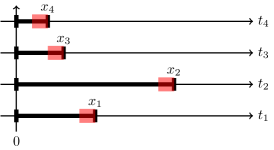
Figure 17: The set $\mathfrak{X}$ over which the Fredholm determinant (5.21) of $\mathbf{1}-\mathcal{K}$ is taken. Highlighted is the right edge of $\mathfrak{X}$, i.e., the subset contributing to the limiting Fredholm determinant. Here $\ell=4$.

Consider the Tracy-Widom phase, the other cases are analogous. The scaling is

$$t_{i}=\theta L+2\mathfrak{w}^{\circ}\mathfrak{d}_{TW}^{2}s_{i}L^{2/3},\qquad x_{i}=\lfloor\mathfrak{h}L+2(\mathfrak{w}^{\circ})^{2}\mathfrak{d}_{TW}^{2}s_{i}L^{2/3}+\mathfrak{w}^{\circ}\mathfrak{d}_{TW}(s_{i}^{2}-r_{i})L^{1/3}\rfloor,$$

where $(\theta,\chi)$ is in the Tracy-Widom phase and $s_{1},\ldots,s_{\ell},r_{1},\ldots,r_{\ell}\in\mathbb{R}$ are fixed. The Fredholm determinant (5.21) expresses the probability $\mathop{\mathrm{Prob}}(\mathcal{H}(t_{i},\chi)>x_{i},\,i=1,\ldots,\ell)$. Fix sufficiently large positive $\kappa_{1},\ldots,\kappa_{\ell}$, and define the right edge $\mathfrak{X}_{re}$ of $\mathfrak{X}$ to be disjoint union of segments from $\mathfrak{h}L+2(\mathfrak{w}^{\circ})^{2}\mathfrak{d}_{TW}^{2}s_{i}L^{2/3}+\mathfrak{w}^{\circ}\mathfrak{d}_{TW}(s_{i}^{2}-\kappa_{i})L^{1/3}$ to $x_{i}$ on each level $t_{i}$. By Proposition 5.8 we have for all $n$:

$$\frac{(-1)^{n}}{n!}\sum_{y^{1},\ldots,y^{n}\in\mathfrak{X}_{re}}\det[\mathcal{K}(y^{p};y^{q})]_{p,q=1}^{n}\\ =(1+O(L^{-1/3}))\,\frac{(-1)^{n}}{n!}\int\ldots\int\det[\mathsf{A}^{\mathrm{ext}}(Y^{p};Y^{q})]_{p,q=1}^{n}\,dh^{1}\ldots dh^{n},$$

where each of the integrals is over $Y^{p}=(s^{p},h^{p})\in\sqcup_{i=1}^{\ell}\{s_{i}\}\times[r_{i},\kappa_{i}]$. The prefactors $(\mathfrak{w}^{\circ}\mathfrak{d}_{TW}L^{1/3})^{-1}$ are absorbed when we pass from sums to integrals due to our scaling. We also ignored the gauge factors in Proposition 5.8 because they do not change the determinants. Taking $\kappa_{i}$ sufficiently large and using the decay of the Airy kernel (e.g., see [TW94]) leads to the desired Fredholm determinant of $\mathbf{1}-\mathsf{A}^{\mathrm{ext}}$. In the BBP and Gaussian regime we use Propositions 5.10 and 5.11, respectively, to get similar convergence with the corresponding limiting kernels. (In the Gaussian phase the right edge has scale $L^{1/2}$ and not $L^{1/3}$).

Let us show that the contribution to the Fredholm determinant is negligible when at least one $y^{p}$ is outside $\mathfrak{X}_{re}$. We again consider only the Tracy-Widom phase as the other ones are analogous. Fix $p_{0}$ such that $y^{p_{0}}$ is summed over $\mathfrak{X}\setminus\mathfrak{X}_{re}$. In (5.21) consider the $n$-th sum, and expand the $n\times n$ determinant as a sum over permutations $\sigma\in S(n)$. In each of the resulting $n!$ terms single out the factor containing $y^{p_{0}}$ in the second place:

$$\prod_{j=1}^{n}\mathcal{K}(y^{j};y^{\sigma(j)})=\cdots\mathcal{K}(y^{p};y^{p_{0}})\cdots.$$ (5.22)

We are interested in $\mathcal{K}(y^{p};y^{p_{0}})$ which is a sum of the additional term and the double contour integral $\mathcal{I}$, cf. (5.1). For $\mathcal{I}$ we use the estimate of Lemma 5.13 (in the Gaussian phase we would need Lemma 5.14). Namely, the sum of the right-hand side of (5.20) over $y^{p_{0}}=(t^{\prime},x^{\prime})$ outside $\mathfrak{X}_{re}$ can be bounded in absolute value by $C(e^{-c_{1}L^{\varepsilon_{1}}}\log L+e^{-c\kappa})$, where $\kappa=\min_{1\leq i\leq\ell}\kappa_{i}$, and this is small for large $L$ as we take large enough $\kappa_{i}$.

The additional term in $\mathcal{K}(y^{p};y^{p_{0}})$ is nonzero when $t^{p}>t^{p_{0}}$ and $x^{p}\geq x^{p_{0}}$. One can see similarly to (5.13) that when $x^{p_{0}}-x^{p}<-\tilde{\kappa}L^{1/3}$ for sufficiently large $\tilde{\kappa}>0$, the additional term is negligible. Otherwise (when $x^{p}$ and $x^{p_{0}}$ are close to each other within a constant multiple of $L^{1/3}$) it is not negligible, and in this case, $y^{p}$ (which we now call $y^{p_{1}}$) is also outside of $\mathfrak{X}_{re}$. We then proceed by finding the factor in (5.22) with $y^{p_{1}}$ in the second place, say, $\mathcal{K}(y^{p_{2}};y^{p_{1}})$. If $t^{p_{2}}>t^{p_{1}}$, this factor can also contribute a non-negligible additional summand if $x^{p_{2}}$ is close to $x^{p_{1}}$, and we can repeat the argument by finding $\mathcal{K}(y^{p_{3}};y^{p_{2}})$. However, due to the indicators in front of the additional term in $\mathcal{K}$, we must take the double contour integral $\mathcal{I}$ from at least one of the $n$ factors in (5.22). Therefore, this procedure of finding non-negligible contributions will eventually terminate and these additional summands are multiplied by an integral factor. When the additional summands are not small, the corresponding $y^{p_{i}}$’s are outside $\mathfrak{X}_{re}$, and thus the integral factor becomes small. We conclude that any non-negligible additional summands are multiplied by at least one double contour integral factor which is asymptotically negligible. This establishes the desired convergence of the Fredholm determinants, and completes the proof of Theorem 4.6. ∎

Proof of Theorem 4.5.

Let us now prove the limit shape theorem that $\lim_{L\to+\infty}L^{-1}\mathcal{H}(\theta,\chi)=\mathfrak{h}(\theta,\chi)$ in probability for each fixed $(\theta,\chi)$. If $(\theta,\chi)$ is in the curved part (Definition 4.1), then this convergence in probability immediately follows from the (single-point) fluctuation results of Theorem 4.6. When $(\theta,\chi)$ is outside the curved part, consider the first particle $x_{1}$ of the continuous space TASEP. Since this particle performs a simple Poisson random walk (in inhomogeneous space), its location satisfies a Law of Large Numbers. Namely, for fixed $\theta>0$:

$$\lim_{L\to+\infty}\mathop{\mathrm{Prob}}\left(|x_{1}(\theta L)-\chi_{e}(\theta)|>\varepsilon\right)=0\quad\textnormal{for all $\varepsilon>0$},$$

where $\chi_{e}(\theta)$ is the unique solution to $\theta=\int_{0}^{\chi}du/\xi(u)$. This implies that $\mathop{\mathrm{Prob}}\left(\mathcal{H}(\theta L,\chi)>\varepsilon L\right)\to 0$ for all $\chi>\chi_{e}(\theta)$. For $\chi=\chi_{e}(\theta)$ the critical point equation (5.2) has a unique solution $\mathfrak{w}^{\circ}=0$, and thus $\mathfrak{h}=0$. One can check that then $G(v)$ (4.7) has a single critical point at $v=0$, and so $\mathcal{H}(\theta L,\chi_{e}(\theta))$ has Gaussian type fluctuations of order $L^{1/2}$ around the limiting value $\mathfrak{h}(\theta,\chi_{e}(\theta))=0$. Thus, the limit shape for the height function $L^{-1}\mathcal{H}$ at $\chi_{e}(\theta)$ is also zero, which completes the proof. ∎

5.5 Fluctuations around a traffic jam

In this subsection we analyze fluctuations in the continuous space TASEP around a down jump of the speed function $\xi(\cdot)$ at $\boldsymbol{\upchi}=1$, see (4.14). For this particular choice of $\xi(\cdot)$ the correlation kernel (5.1) has the form

$$\begin{split}&\mathcal{K}(t,x;t^{\prime},x^{\prime})=-\mathbf{1}_{t>t^{\prime}}\mathbf{1}_{x\geq x^{\prime}}\frac{(t-t^{\prime})^{x-x^{\prime}}}{(x-x^{\prime})!}\\ &\hskip 80.0pt+\frac{1}{(2\pi{\mathbf{i}\mkern 1.0mu})^{2}}\oint\oint\frac{dwdz}{z(z-w)}\exp\left\{L\bigl{(}G(w;\tfrac{t^{\prime}}{L},\chi,\tfrac{x^{\prime}}{L})-G(z;\tfrac{t}{L},\chi,\tfrac{x}{L})\bigr{)}\right\}\frac{1-z}{1-w},\end{split}$$ (5.23)

where $G$ for $\chi>1$ (the regime we’re interested in) is given by

$$G(v;\theta,\chi,h)=-\theta v+h\log v+\frac{1}{1-v}+\frac{\chi-1}{1-2v}.$$

The $z$ contour is a small circle around $0$, and the $w$ contour encircles $1/2$ and $1$.

The scaled time is assumed to be critical $\theta_{\mathsf{cr}}=12$ (given by the right-hand side of (4.13)). Recall that as $\theta$ passes $\theta_{\mathsf{cr}}$ the limit shape loses continuity at $\boldsymbol{\upchi}=1$. Set

$$\chi-1=10\upepsilon>0$$

(the factor $10$ is convenient in the formulas below) and let $\upepsilon=\upepsilon(L)\to 0$ as $L\to+\infty$. Let us expand the double critical point $\mathfrak{w}^{\circ}$ of $G$ and the limit shape $\mathfrak{h}$ in powers of $\upepsilon$.

Lemma 5.15.

For small $\upepsilon>0$, the double critical point and the limiting height function behave as

$$\mathfrak{w}^{\circ}(12,1+10\upepsilon) =\frac{1}{2}-\frac{1}{2}\,\upepsilon^{\frac{1}{4}}-\frac{1}{5}\,\upepsilon^{\frac{1}{2}}+\frac{7}{100}\,\upepsilon^{\frac{3}{4}}+\frac{191}{2000}\,\upepsilon+O(\upepsilon^{\frac{5}{4}});$$ (5.24)

$$\mathfrak{h}(12,1+10\upepsilon) =4-10\upepsilon^{\frac{1}{2}}+6\upepsilon^{\frac{3}{4}}+O(\upepsilon^{\frac{5}{4}}).$$ (5.25)

Proof.

The double critical point $\mathfrak{w}^{\circ}$ satisfies equation (5.2) which for our particular $\xi(\cdot)$ and $\theta=12$ becomes (after removing the denominator $(v-1)^{3}(2v-1)^{3}$)

$$-11+20\upepsilon+(103-20\upepsilon)v-30(13+2\upepsilon)v^{2}+20(38+5\upepsilon)v^{3}-40(20+\upepsilon)v^{4}+432v^{5}-96v^{6}=0.$$ (5.26)

When $\upepsilon=0$, (5.26) has root $v=\frac{1}{2}$ of multiplicity $4$ which after taking the denominator into account corresponds to a single root.

Figure 18: Behavior of four roots of (5.26) in the complex plane which become $v=\frac{1}{2}$ for $\upepsilon=0$.

For small $\upepsilon>0$ there are four roots close to $\frac{1}{2}$ two of which are complex conjugate and two of which are real, see Figure 18. We are interested in the unique root $\mathfrak{w}^{\circ}\in(0,\frac{1}{2})$. Using Implicit Function Theorem to find derivatives of $\mathfrak{w}^{\circ}$ in $\upepsilon$, we get the desired expansion (5.24). The expansion of $\mathfrak{h}$ is obtained using (5.3) which now takes the form

$$\mathfrak{h}(12,1+10\upepsilon)=12\mathfrak{w}^{\circ}-\frac{\mathfrak{w}^{\circ}}{(1-\mathfrak{w}^{\circ})^{2}}-\upepsilon\,\frac{5\mathfrak{w}^{\circ}}{\left(\frac{1}{2}-\mathfrak{w}^{\circ}\right)^{2}}$$

together with the expansion of $\mathfrak{w}^{\circ}$. This completes the proof. ∎

Expansion (5.25) implies that $\frac{\partial}{\partial\upepsilon}\mathfrak{h}(12,1+10\upepsilon)\big{|}_{\upepsilon=0}=-\infty$ but $\mathfrak{h}$ is continuous at $\boldsymbol{\upchi}=1$ (and $\mathfrak{h}(12,1)=4$). This behavior corresponds to the middle picture in Figure 13.

In the rest of the subsection we prove Theorem 4.7. The analysis of fluctuations of the random height function is similar to Sections 5.2, 5.3 and 5.4. The main difference is in the asymptotic expansion in the exponent under the integral in the kernel $\mathcal{K}$ (5.23) which leads to different limiting kernels. The large $L$ behavior of this exponent depends on the relative speeds at which $\upepsilon\to 0$ and $L\to\infty$. To shorten notation let, by agreement, $\mathfrak{w}^{\circ}$, $\mathfrak{h}$, and $\mathfrak{d}_{TW}$ depend on the parameters $\theta=12$ and $\chi=1+10\upepsilon$. The corresponding $\upepsilon=0$ pre-slowdown values $\mathfrak{w}^{\circ}(12,1)=\frac{1}{2}$, $\mathfrak{h}(12,1)=4$, and $\mathfrak{d}_{TW}(12,1)=4\cdot 5^{1/3}$ will be used explicitly.

We consider three cases based on how $\upepsilon$ compares with $L^{-4/3}$. Indeed, $(L^{-4/3})^{1/4}=L^{-1/3}$ corresponds to the scaling of the integration variables around the double critical point $\mathfrak{w}^{\circ}$ which itself is close to $1/2$ within $\upepsilon^{1/4}$, see (5.24). The interplay of these two effects leads to the three cases below.

5.5.1 Close to the slowdown

Let $0<\upepsilon\ll L^{-\frac{4}{3}-\gamma}$ for some $\gamma>0$. Scale the parameters as follows (note the differences with (5.6))

$$\begin{split}t&=12L+\mathfrak{w}^{\circ}\mathfrak{d}_{TW}^{2}2^{-1/3}s^{\prime}L^{2/3},\qquad t^{\prime}=12L+\mathfrak{w}^{\circ}\mathfrak{d}_{TW}^{2}2^{-1/3}sL^{2/3},\\ x&=\lfloor 4L+(\mathfrak{w}^{\circ})^{2}\mathfrak{d}_{TW}^{2}2^{-1/3}s^{\prime}L^{2/3}+\mathfrak{w}^{\circ}\mathfrak{d}_{TW}(s^{\prime 2}-h^{\prime})2^{-2/3}L^{1/3}\rfloor,\\ x^{\prime}&=\lfloor 4L+(\mathfrak{w}^{\circ})^{2}\mathfrak{d}_{TW}^{2}2^{-1/3}sL^{2/3}+\mathfrak{w}^{\circ}\mathfrak{d}_{TW}(s^{2}-h)2^{-2/3}L^{1/3}\rfloor,\\ z&=\frac{1}{2}+\frac{\tilde{z}}{2\cdot 10^{1/3}L^{1/3}},\qquad\qquad w=\frac{1}{2}+\frac{\tilde{w}}{2\cdot 10^{1/3}L^{1/3}},\end{split}$$ (5.27)

where $\tilde{z},\tilde{w}$ belong to the Airy integration contours as in Figure 15. One can check that

$$L\bigl{(}G(w;\tfrac{t^{\prime}}{L},1+10\upepsilon,\tfrac{x^{\prime}}{L})-G(z;\tfrac{t}{L},1+10\upepsilon,\tfrac{x}{L})\bigr{)}\\ =(\textnormal{gauge terms})+\frac{\tilde{w}^{3}}{3}-s\tilde{w}^{2}-(h-s^{2})\tilde{w}-\frac{\tilde{z}^{3}}{3}+s^{\prime}\tilde{z}^{2}+(h^{\prime}-s^{\prime 2})\tilde{z}+o(1),$$ (5.28)

where “$(\textnormal{gauge terms})$” stand for terms which do not depend on $\tilde{z},\tilde{w}$ and can be removed by a suitable gauge transformation of the kernel (cf. Remark 5.9). These terms do not affect the asymptotics of probabilities in question, and we do not write them down explicitly. One can also check that the gauge terms coming from the non-integral summand in (5.23) are the same as the ones arising from the integral. Moreover, the prefactor $10^{-1/3}L^{-1/3}$ in front of the non-integral summand is the same as $\frac{1}{2}\cdot 2\cdot 10^{-1/3}L^{-1/3}$ coming from the change of variables in the double contour integral, and also coincides with $\mathfrak{w}^{\circ}\mathfrak{d}_{TW}2^{-2/3}L^{-1/3}$ corresponding to rescaling the space variable $x$ to $h$. Repeating the rest of the argument from Sections 5.2, 5.3 and 5.4 we see that when $\chi=1+10\upepsilon$ is close to the slowdown of $\xi(\cdot)$ at $1$, the fluctuations of the height function around the pre-slowdown value $\mathfrak{h}(12,1)=4$ are given by the Airy kernel.

5.5.2 Far from the slowdown

Let $\upepsilon\gg L^{-\frac{4}{3}+\gamma}$ for some $\gamma\in(0,\frac{4}{3})$. Consider the scaling

$$\begin{split}t&=12L+2\mathfrak{w}^{\circ}\mathfrak{d}_{TW}^{2}s^{\prime}L^{2/3},\qquad x=\lfloor\mathfrak{h}L+2(\mathfrak{w}^{\circ})^{2}\mathfrak{d}_{TW}^{2}s^{\prime}L^{2/3}+\mathfrak{w}^{\circ}\mathfrak{d}_{TW}(s^{\prime 2}-h^{\prime})L^{1/3}\rfloor;\\ t^{\prime}&=12L+2\mathfrak{w}^{\circ}\mathfrak{d}_{TW}^{2}sL^{2/3},\qquad x^{\prime}=\lfloor\mathfrak{h}L+2(\mathfrak{w}^{\circ})^{2}\mathfrak{d}_{TW}^{2}sL^{2/3}+\mathfrak{w}^{\circ}\mathfrak{d}_{TW}(s^{2}-h)L^{1/3}\rfloor;\\ z&=\mathfrak{w}^{\circ}+\frac{\tilde{z}}{\mathfrak{d}_{TW}L^{1/3}},\qquad\qquad w=\mathfrak{w}^{\circ}+\frac{\tilde{w}}{\mathfrak{d}_{TW}L^{1/3}}.\end{split}$$

The new integration variables $\tilde{z},\tilde{w}$ belong to the contours as in Figure 15. This scaling is the same as in the general Tracy-Widom fluctuation regime (5.6) but the coefficients also depend on $L$. That is, in contrast with (5.27) here we include corrections of order larger than $\upepsilon^{1/4}\gg L^{-1/3}$ directly into $t,x,t^{\prime},x^{\prime}$ and the integration variables. One can readily check that with this scaling the same expansion (5.28) holds (with different gauge terms). The gauge terms coming from the additional summand in (5.23) are also compatible with the ones in the integral. In this way we again get the Airy kernel describing the fluctuations.

5.5.3 Critical scale at the traffic jam

This case arises when smaller order terms in $\mathfrak{w}^{\circ}(12,1+10\upepsilon)$, $\mathfrak{h}(12,1+10\upepsilon)$, and $\mathfrak{d}_{TW}(12,1+10\upepsilon)$ coincide in scale with the natural Airy corrections of orders $L^{-1/3}$ and $L^{-2/3}$. Let $\upepsilon=10^{-4/3}\delta L^{-4/3}$, where $\delta>0$ is fixed. Consider the scaling

$$\begin{split}t&=12L+\mathfrak{w}^{\circ}\mathfrak{d}_{TW}^{2}2^{-1/3}s^{\prime}L^{2/3},\qquad t^{\prime}=12L+\mathfrak{w}^{\circ}\mathfrak{d}_{TW}^{2}2^{-1/3}sL^{2/3},\\ x&=\lfloor 4L+(\mathfrak{w}^{\circ})^{2}\mathfrak{d}_{TW}^{2}2^{-1/3}s^{\prime}L^{2/3}+\mathfrak{w}^{\circ}\mathfrak{d}_{TW}(s^{\prime 2}+2s^{\prime}\delta^{1/4}-h^{\prime})2^{-2/3}L^{1/3}\rfloor,\\ x^{\prime}&=\lfloor 4L+(\mathfrak{w}^{\circ})^{2}\mathfrak{d}_{TW}^{2}2^{-1/3}sL^{2/3}+\mathfrak{w}^{\circ}\mathfrak{d}_{TW}(s^{2}+2s\delta^{1/4}-h)2^{-2/3}L^{1/3}\rfloor,\\ z&=\frac{1}{2}+\frac{\tilde{z}}{2\cdot 10^{1/3}L^{1/3}},\qquad\qquad w=\frac{1}{2}+\frac{\tilde{w}}{2\cdot 10^{1/3}L^{1/3}},\end{split}$$ (5.29)

where $\tilde{z},\tilde{w}$ belong to the Airy contours (Figure 15). We have the following expansion:

$$L\bigl{(}G(w;\tfrac{t^{\prime}}{L},1+10\upepsilon,\tfrac{x^{\prime}}{L})-G(z;\tfrac{t}{L},1+10\upepsilon,\tfrac{x}{L})\bigr{)}\\ =(\textnormal{gauge terms})+\frac{\tilde{w}^{3}}{3}-s\tilde{w}^{2}-(h-s^{2})\tilde{w}-\frac{\tilde{z}^{3}}{3}+s^{\prime}\tilde{z}^{2}+(h^{\prime}-s^{\prime 2})\tilde{z}+\frac{\delta}{\tilde{z}}-\frac{\delta}{\tilde{w}}+o(1).$$ (5.30)

The additional summand in (5.23) has the expansion:

$$-\mathbf{1}_{t>t^{\prime}}\mathbf{1}_{x\geq x^{\prime}}\frac{(t-t^{\prime})^{x-x^{\prime}}}{(x-x^{\prime})!}=-\mathbf{1}_{s^{\prime}>s}\exp\{\textnormal{gauge terms}\}\,\frac{\exp\left\{-\frac{(h-h^{\prime}-s^{2}+s^{\prime 2})^{2}}{4(s^{\prime}-s)}\right\}}{10^{1/3}L^{1/3}\sqrt{4\pi(s^{\prime}-s)}}$$

with the same gauge terms as in (5.30). We see that the kernel is approximated by the deformed Airy₂ kernel defined in Section C.3. The rest of the argument for convergence of fluctuations can be copied from the proofs in the Tracy-Widom phase in Sections 5.2, 5.3 and 5.4. This completes the proof of Theorem 4.7.

5.5.4 Remark. Relation to deformations of the Airy kernel from [BP08]

The deformed Airy kernel that we obtain arises in the edge scaling limit of a certain multiparameter Wishart-like ensemble of random matrices in the spirit of [BP08]. In that paper the authors consider an Airy-like time-dependent correlation kernel with two finite sets of real parameters. In order to arrive at the kernel of the form $\widetilde{\mathsf{A}}^{\mathrm{ext},\delta}$ (C.6) one needs to consider two infinite sequences of perturbation parameters $x_{i},y_{j}$, and perform a double limit transition. This construction is essentially described in Remark 2 in [BP08], and our kernel corresponds to setting all parameters except $c^{-}$ to zero.

6 Homogeneous doubly geometric corner growth

In this section we consider the limit shape and fluctuations of the homogeneous DGCG model (defined in Section 1.2). Our results are one-parameter deformations of the corresponding results for the celebrated geometric corner growth (equivalently, geometric last-passage percolation) model.

Set $a_{i}\equiv 1$, $\beta_{t}\equiv\beta>0$, and $\nu_{j}\equiv\nu\in[-\beta,1)$, and let $H_{T}(N)$ denote the height function in this homogeneous DGCG model. Let $L\to+\infty$ be a large parameter, the location and time scale linearly as $N=\lfloor\eta L\rfloor$, $T=\lfloor\tau L\rfloor$, where $\eta$ and $\tau$ are the scaled location and time, respectively. Fix $\tau>0$ and define the limiting height function $\eta\mapsto\mathsf{h}(\tau,\eta)$ as the following parametric curve:

$$\eta(z)=\tau\,\frac{\beta(1-z)^{2}(1-z\nu)^{2}}{(1-\nu)(1-z^{2}\nu)(1+z\beta)^{2}},\qquad\mathsf{h}(z)=\tau\,\frac{\beta z^{2}\left(\beta(1-z^{2}\nu)+\nu(1-2z)+1\right)}{(1+\beta z)^{2}(1-z^{2}\nu)},$$ (6.1)

where $0\leq z\leq 1$. See Figure 19 for examples. In more detail, we say that $(\tau,\eta)$ is in the curved part if $\tau\beta>\eta(1-\nu)$. One can show that for $(\tau,\eta)$ in the curved part there exists a unique solution to $\eta=\eta(z)$ in $z$ belonging to $(0,1)$.

Figure 19: Limit shapes for varying parameter $\nu$. The case $\nu=-\beta=-\frac{1}{4}$ coincides with the limit shape parabola in the geometric corner growth model.

Keeping the same parameter $z$ (with $z\in(0,1)$ corresponding to the curved part), define

$$\mathsf{d}(z):=\Biggl{[}\frac{(1-\nu)\eta(z)}{z(1+z\beta)(1-z)^{3}(1-\nu z)^{3}}\Bigl{(}\beta+1+\nu-3z\nu(1+z\beta)+\beta z^{3}\nu(1+\nu)+z^{3}\nu^{2}\Bigr{)}\Biggr{]}^{1/3}.$$

One can show that $\mathsf{d}(z)>0$. Also define

$$\mathscr{A}(z):=\frac{2z\mathsf{d}(z)^{2}(1+\beta z)^{2}}{\beta},\qquad\mathscr{B}(z):=2z\mathsf{d}(z)(1+\beta z),\qquad\mathscr{C}(z):=z\mathsf{d}(z).$$

Theorem 6.1.

As $L\to+\infty$, for all $\tau,\eta>0$ the scaled DGCG height function $L^{-1}H_{\lfloor\tau L\rfloor}(\lfloor\eta L\rfloor)$ converges to $\mathsf{h}(\tau,\eta)$ in probability (some examples are given in Figure 20).

Fix $(\tau,\eta)=(\tau,\eta(z))$ in the curved part corresponding to some parameter value $z\in(0,1)$ (recall that $\eta(z),\mathsf{h}(z)$ also depend on $\tau$). For any $s_{1},\ldots,s_{\ell},r_{1},\ldots,r_{\ell}\in\mathbb{R}$ we have

$$\lim_{L\to+\infty}\mathop{\mathrm{Prob}}\left(\frac{H_{\lfloor\tau L+\mathscr{A}(z)s_{i}L^{2/3}\rfloor}(\lfloor\eta(z)L\rfloor)-L\mathsf{h}(z)-\mathscr{B}(z)s_{i}L^{2/3}}{\mathscr{C}(z)L^{1/3}}>s_{i}^{2}-r_{i},\,i=1,\ldots,\ell\right)\\ =\det\left(\mathbf{1}-\mathsf{A}^{\mathrm{ext}}\right)_{\sqcup_{i=1}^{\ell}\{s_{i}\}\times(r_{i},+\infty)},$$

where $\mathsf{A}^{\mathrm{ext}}$ is the extended Airy kernel (Section C.1). In particular, for $\ell=1$ we have convergence to the Tracy-Widom GUE distribution:

$$\lim_{L\to+\infty}\mathop{\mathrm{Prob}}\left(\frac{H_{\lfloor\tau L\rfloor}(\lfloor\eta(z)L\rfloor)-L\mathsf{h}(z)}{\mathscr{C}(z)L^{1/3}}>-r\right)=F_{GUE}(r),\qquad r\in\mathbb{R}.$$

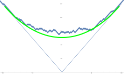
(a)	(b)
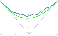
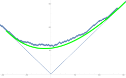
(c)	(d)

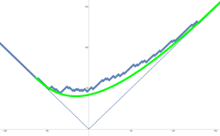
Figure 20: Simulations of the homogeneous DGCG with $\beta=\frac{1}{4}$ (as in Figure 19), unscaled time $T=500$, and (a) $\nu=-\frac{1}{4}$ (parabolic limit shape), (b) $\nu=0$, (c) $\nu=\frac{1}{4}$, (d) $\nu=\frac{1}{2}$. These figures use the interpretation of DGCG as parallel TASEP (Section A.1) and are thus rotated by $45^{\circ}$.

Remark 6.2 (Reduction to classical corner growth).

For $\nu=-\beta$ the homogeneous DGCG model turns into the standard corner growth model. Explicit limit shape in the simpler exponential corner growth model goes back to [Ros81]. For the geometric corner growth, the limit shape was obtained in [JPS98], [CEP96], and [Sep98] using various approaches. GUE Tracy-Widom fluctuations for the geometric corner growth are due to Johansson [Joh00].

For $\nu=-\beta$ the curve (6.1) becomes

$$\eta(z)=\frac{\tau\beta(1-z)^{2}}{(1+\beta)(1+z^{2}\beta)},\qquad\mathsf{h}(z)=\frac{\tau\beta z^{2}}{1+z^{2}\beta},$$

which after excluding $z$ reduces to

$$\tau=\frac{\eta+\mathsf{h}+2\sqrt{\mathsf{q}\mathsf{h}\eta}}{1-\mathsf{q}},$$

under the identification of the parameters $\beta=\mathsf{q}^{-1}-1$, where $\mathsf{q}\in(0,1)$ is the parameter of the geometric waiting time in the notation of [Joh00]. Setting $\eta=1$ and $\mathsf{h}=\gamma$ turns the right-hand side into the limiting value of the last-passage time $N^{-1}G^{*}(\lfloor\gamma N\rfloor,N)$ from [Joh00]. The latter corresponds to the parabolic limit shape in the geometric corner growth / last-passage percolation. See Figures 19 and 20 for an illustration of how the DGCG limit shapes form a one-parameter extension of this parabola.

In the rest of the section we outline a proof of Theorem 6.1, mainly focusing on the contour estimates required for the steepest descent analysis. In view of Remark 6.2, we will not consider the particular case $\nu=-\beta$ extensively studied previously, and will assume that $\nu\in(-\beta,1)$.

First, note that for $\nu<0$ the connection of DGCG to Schur measures decribed in Section 3.2 breaks since Schur processes are not well-defined for negative parameters. However, both the homogeneous DGCG model and the limit shape curve (6.1) depend on $\nu\in[-\beta,1)$ in a continuous way. Moreover, the kernel $\mathsf{K}_{N}$ (3.16) and its Fredholm determinants like (3.19) clearly make sense for negative $\nu$. The probability distribution of the height function $H_{T}(N)$ of the homogeneous DGCG depends on $\nu$ in a polynomial (hence analytic) way. Therefore, we can analytically continue formulas expressing the distribution of $H_{T}(N)$ as Fredholm determinants of $\mathsf{K}_{N}$ into the range $\nu\in(-\beta,1)$. This allows us to study the asymptotic behavior of the homogeneous DGCG for $\nu\in(-\beta,1)$ by analyzing the same kernel $\mathsf{K}_{N}$.

Let us write down the specialization of $\mathsf{K}_{N}$ to the homogeneous case:

$$\begin{split}&\mathsf{K}_{N}(T,x;T^{\prime},x^{\prime})=-\frac{\mathbf{1}_{T>T^{\prime}}\mathbf{1}_{x\geq x^{\prime}}}{2\pi{\mathbf{i}\mkern 1.0mu}}\oint\frac{(1+\beta z)^{T-T^{\prime}}}{z^{x-x^{\prime}+1}}\,dz\\ &\hskip 60.0pt+\frac{1}{(2\pi{\mathbf{i}\mkern 1.0mu})^{2}}\oint\oint\frac{dz\,dw}{z-w}\frac{w^{x^{\prime}+N}}{z^{x+N+1}}\left(\frac{1-w\nu}{1-z\nu}\right)^{N-1}\frac{(1+\beta_{t}z)^{T}}{(1+\beta_{t}w)^{T^{\prime}}}\left(\frac{1-z}{1-w}\right)^{N},\end{split}$$ (6.2)

The $z$ contour is a small positive circle around $0$ which does not include $1/\nu$, and the $w$ contour is a small positive circle around $1$ which is to the right of $0$, $-1/\beta$, and the $z$ contour.

The asymptotic analysis of $\mathsf{K}_{N}$ follows essentially the same steps as performed for the continuous space TASEP in Section 5. That is, we write $\mathsf{K}_{N}$ as in (5.1) with the function in the exponent under the double integral looking as

$$S_{L}(z)=S_{L}(z;T,N,h):=\frac{h}{L}\log z+\frac{N-1}{L}\log(1-\nu z)-\frac{T}{L}\log(1+\beta z)-\frac{N}{L}\log(1-z),$$

where $h=x+N$. The scaling of the parameters $T=\lfloor\tau L\rfloor$, $N=\lfloor\eta L\rfloor$ means that we can modify the function $S_{L}$ to be

$$S_{L}(z)=\frac{h}{L}\log z+\eta\log(1-\nu z)-\tau\log(1+\beta z)-\eta\log(1-z).$$ (6.3)

Indeed, the difference in the exponent is either small or can be removed by a suitable gauge transformation.

We find the double critical point $z=\mathsf{z}_{L}$ of $S_{L}(z)$, and deform the integration contours so that the behavior of the double contour integral is dominated by a small neighborhood of $\mathsf{z}_{L}$. To complete the argument we need to show the existence of steep ascent/descent integration contours. That is, we find new contours $\gamma_{\pm}$ such that $\mathop{\mathrm{Re}}S_{L}(z)$ attains its minimum on $\gamma_{+}$ at $z=\mathsf{z}_{L}$, and $\mathop{\mathrm{Re}}S_{L}(w)$ attains its maximum on $\gamma_{-}$ at $w=\mathsf{z}_{L}$.

In the sequel we assume that $(\tau,\eta)$ is in the curved part: $\tau\beta>\eta(1-\nu)$. Moreover, we will always assume that $h<\tau L$ as the corresponding pre-limit inequality $H_{T}(N)\leq T$ holds almost surely by the very definition of the DGCG model.

One readily sees that $S_{L}(z)$ has three critical points, up to multiplicity, since the numerator in $S^{\prime}_{L}(z)$ is a cubic polynomial. In the curved part there exists $\mathsf{h}_{L}$ such that $S_{L}(z;T,N,\mathsf{h}_{L})$ has a double critical point $\mathsf{z}_{L}\in(0,1)$. Taking this double critical point as a parameter of the limit shape and expressing $\mathsf{h}$ and $\eta$ (for fixed $\tau$) through this critical point, we arrive at the formulas for the limit shape (6.1).

The next two Lemmas 6.3 and 6.4 determine the location of the third critical point of $S_{L}$ (which must also be real).

Lemma 6.3.

The function $S_{L}$ (6.3) has the following limits:

$$\begin{split}\lim_{z\rightarrow\infty}\mathop{\mathrm{Re}}S_{L}(z)=\lim_{z\rightarrow\nu^{-1}}&\mathop{\mathrm{Re}}S_{L}(z)=\lim_{z\rightarrow 0}\mathop{\mathrm{Re}}S_{L}(z)=-\infty,\\ \lim_{z\rightarrow-\beta^{-1}}\mathop{\mathrm{Re}}S_{L}(z)&=\lim_{z\rightarrow 1}\mathop{\mathrm{Re}}S_{L}(z)=\infty.\end{split}$$ (6.4)

Proof.

This follows from the limits $\log|v|\rightarrow-\infty$ as $v\rightarrow 0$ and $\log|v|\rightarrow\infty$ as $v\rightarrow\infty$. The signs of the infinities are determined by the signs of the parameters. At $v\to\infty$ we use $h/L<\tau$. ∎

Lemma 6.4.

The function $S_{L}$ (6.3) has a real critical point $v_{0}\in(-\infty,\nu^{-1})$.

Proof.

It suffices to show that $S_{L}^{\prime}(v_{1})<0$ and $S_{L}^{\prime}(v_{2})>0$ for a pair of real points $v_{1},v_{2}\in(-\infty,1/\nu)$. We have that $S_{L}^{\prime}(z)\rightarrow-\infty$ as $v\rightarrow(1/\nu)^{-}$. This establishes the existence of $v_{1}\in(-\infty,1/\nu)$ such that $S_{L}^{\prime}(v_{1})<0$. Also, we have that $vS_{L}^{\prime}(v)\rightarrow h/L-\tau<0$ as $v\rightarrow-\infty$. This establishes the existence of $v_{2}\in(-\infty,1/\nu)$, near negative infinity on the real axis, such that $S_{L}^{\prime}(v_{2})>0$. Therefore, there is $v_{0}\in(v_{2},v_{1})$ such that $S_{L}^{\prime}(v_{0})=0$. ∎

As the new contours $\gamma_{\pm}$ we take the steepest ascent/descent paths. Recall that for a meromorphic function $f:\mathbb{C}\rightarrow\mathbb{C}$, an oriented path $\gamma:[0,1]\rightarrow\mathbb{C}$ is a steepest path with base point $z_{0}\in\mathbb{C}$ if $\gamma$ is smooth, travels along the gradient of $\mathop{\mathrm{Re}}f$ (i.e. $\gamma^{\prime}(t)\cdot\nabla(\mathop{\mathrm{Re}}f)|_{z=\gamma(t)}=\lambda\gamma^{\prime}(t)$), and $\gamma(0)=z_{0}$. If $\mathop{\mathrm{Re}}f$ is increasing or decreasing along $\gamma$, we say that $\gamma$ is a steepest ascent or descent path, respectively.

Proposition 6.5.

Consider the function $S_{L}(z;\lfloor\tau L\rfloor,\lfloor\eta L\rfloor,\mathsf{h}_{L})$ which has a double critical point at $z=\mathsf{z}_{L}$. There is a pair of steepest ascent paths with base point $\mathsf{z}_{L}$, denoted as $\gamma_{+}^{(1)}$ and $\gamma_{+}^{(2)}$ (symmetric with respect to $\mathbb{R}$), so that $\gamma_{+}:=\gamma^{(1)}_{+}\cup\gamma^{(2)}_{+}$ is a simple closed curve enclosing the origin and traveling through $-\beta^{-1}$. There is a pair of steepest descent paths with base point $\mathsf{z}_{L}$, denoted as $\gamma_{-}^{(1)}$ and $\gamma_{-}^{(2)}$ (also symmetric with respect to $\mathbb{R}$), so that $\gamma_{-}:=\gamma^{(1)}_{-}\cup\gamma^{(2)}_{-}$ is a simple closed curve (on the Riemann sphere) that travels through a real point in $[-\infty,1/\nu]$. See Figure 21 for an illustration.

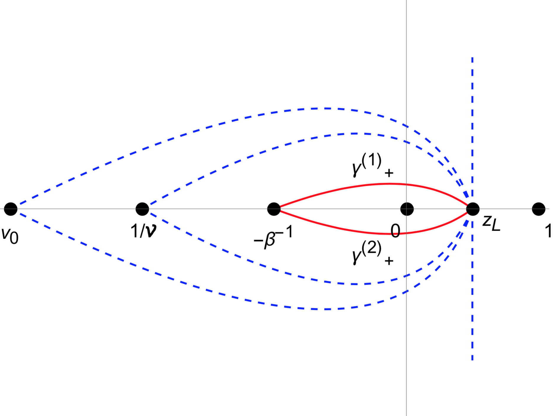
Figure 21: Steepest ascent/descent contours for $S_{L}(z;T,N,\mathsf{h}_{L})$. The steepest ascent contours comprising $\gamma_{+}$ are solid red, and possible options for the steepest descent contours comprising $\gamma_{-}$ are dashed blue.

The contours $\gamma_{+}$ and $\gamma_{-}$ are assumed to have positive (counterclockwise) orientation.

Remark 6.6.

In the proofs in Section 5 we took concrete integration contours which were not the steepest, and this required estimating the derivative of $\mathop{\mathrm{Re}}S_{L}$ along the contours. For the relatively simpler function (6.3) we can in fact understand the global configuration of the steepest ascent/descent contours, and this allows to avoid concrete estimates of derivatives of $\mathop{\mathrm{Re}}S_{L}$.

Proof of Proposition 6.5.

Since $S_{L}(z)$ is analytic at the critical point $\mathsf{z}_{L}$, we know the local shape of all of the steepest paths with base point $\mathsf{z}_{L}$. To establish the global structure of the paths we use the following properties:

1. $\mathop{\mathrm{Re}}S_{L}(z)=\mathop{\mathrm{Re}}S_{L}(\bar{z})$;

2. steepest paths for a meromorphic function only intersect at critical points or singularities;

3. the end point of any steepest path is a critical point, or a singularity, or infinity.

The first property implies that $\gamma_{+}^{(1)}$ and $\gamma_{+}^{(2)}$ are symmetric with respect to the real line, and the same for $\gamma_{-}^{(1)}$ and $\gamma_{-}^{(2)}$.

Since $\mathsf{z}_{L}$ is a double critical point and $S_{L}^{\prime\prime\prime}(\mathsf{z}_{L})>0$, there are six distinct steepest descent paths with base point $\mathsf{z}_{L}$: an ascent path along the real axis from $\mathsf{z}_{L}$ to $1$, a descent path along the real axis from $\mathsf{z}_{L}$ to $0$, and four other paths which we denote by $\gamma_{+}^{(1)}$, $\gamma_{+}^{(2)}$, $\gamma_{-}^{(2)}$, and $\gamma_{-}^{(1)}$ (in counterclockwise order). We know that the paths $\gamma_{+}^{(1)}$ and $\gamma_{+}^{(2)}$ are (locally) to the left of $\gamma_{-}^{(1)}$ and $\gamma_{-}^{(2)}$.

The end point of $\gamma_{-}^{(1)}$ must be a singularity or a critical point. By the limits of Lemma 6.3 and recalling the simple critical point $v_{0}\in(-\infty,1/\nu)$ from Lemma 6.4, the end point of $\gamma_{-}^{(1)}$ must be $0$, $1/\nu$, $v_{0}$, or $\infty$. It follows that $\gamma_{-}=\gamma_{-}^{(1)}\cup\gamma_{-}^{(2)}$ must be a simple closed curve (on the Riemann sphere) passing through one of the points $0$, $1/\nu$, $v_{0}$, or $\infty$. The union $\gamma_{+}=\gamma_{+}^{(1)}\cup\gamma_{+}^{(2)}$ of the steepest ascent paths with base point $\mathsf{z}_{L}$ is a simple closed curve passing through $-1/\beta$ or $1$.

The curves $\gamma_{+}$ and $\gamma_{-}$ cannot intersect outside $\mathbb{R}$ as this would imply existence of additional imaginary critical points or singularities of $S_{L}(z)$, which is not possible. Thus, $\gamma_{+}$ cannot pass through $1$, and $\gamma_{-}$ cannot pass through $0$. We are left with the steepest paths described by the statement of this proposition, which are depicted in Figure 21. ∎

To finish the proof of Theorem 6.1, it remains to show that the $z$ and $w$ integration contours in the kernel $\mathsf{K}_{N}$ (6.2) can be deformed to $\gamma_{+}$ and $\gamma_{-}$, respectively.

The old $z$ contour is a small circle around $0$, and $-\beta^{-1}$ is not a pole in $z$. Therefore, we can replace the $z$ contour by $\gamma_{+}$ without picking any residues. We then deform the $w$ contour to $(-\gamma_{-})$ by passing over infinity in the Riemann sphere. In this deformation, the only possible residue contribution can come from infinity since the integrand is analytic elsewhere along the deformation. Counting the powers of $w$ as $w\to\infty$ in (6.2) (or recalling that $S_{L}(w)\to-\infty$ as $w\to\infty$) we conclude that the integrand does not have a residue at $w=\infty$, and thus the deformation can be performed.

The orientation of $\gamma_{-}$ is negative after the deformation. This sign is the same extra factor of $(-1)$ arising in the proof of Proposition 5.8. Taking this orientation into account we see that the limiting Airy fluctuation kernel has the correct sign. We omit the straightforward computation of the constants in the Airy kernel limit in Theorem 6.1.

Appendix A Equivalent models

Here we discuss a number of equivalent combinatorial formulations of our discrete DGCG model. For simplicity we consider only fully homogeneous models with $a_{i}\equiv a$, $\nu_{j}\equiv\nu$, $\beta_{t}\equiv\beta$. In Section A.4 we also describe an equivalent formulation of the (homogeneous) continuous space TASEP.

A.1 Parallel TASEP with geometric-Bernoulli jumps

Let us interpret the doubly geometric corner growth $H_{T}(N)$ as a TASEP-like particle system.

Definition A.1.

The geometric-Bernoulli random variable $\mathsf{g}\in\mathbb{Z}_{\geq 0}$ (gB variable, for short; notation $\mathsf{g}\sim\mathrm{gB}(a\beta,\nu)$) is a random variable with distribution

$$\mathop{\mathrm{Prob}}(\mathsf{g}=j):=\frac{\mathbf{1}_{j=0}}{1+a\beta}+\frac{a\beta\,\mathbf{1}_{j\geq 1}}{1+a\beta}\left(\frac{\nu+a\beta}{1+a\beta}\right)^{j-1}\frac{1-\nu}{1+a\beta},\qquad j\in\mathbb{Z}_{\geq 0}.$$

Definition A.2.

The geometric-Bernoulli Totally Asymmetric Simple Exclusion Process (gB-TASEP, for short) is a discrete time Markov chain $\{\vec{G}(T)\}_{T\in\mathbb{Z}_{\geq 0}}$ on the space of particle configurations $\vec{G}=(G_{1}>G_{2}>\ldots)$ in $\mathbb{Z}$, with at most one particle per site allowed, and the step initial condition $G_{i}(0)=-i$, $i=1,2,\ldots$.

The dynamics of gB-TASEP proceeds as follows. At each discrete time step, each particle $G_{j}$ with an empty site to the right (almost surely there are finitely many such particles at any finite time) samples an independent random variable $\mathsf{g}_{j}\sim\mathrm{gB}(a\beta,\nu)$, and jumps by $\min(\mathsf{g}_{j},G_{j-1}-G_{j}-1)$ steps (with $G_{0}=+\infty$ by agreement). See Figure 4 (in the Introduction) for an illustration.

Proposition A.3.

Let $H_{T}(N)$ be the DGCG height function. Then for all $T\in\mathbb{Z}_{\geq 0}$ and $N\in\mathbb{Z}_{\geq 1}$ we have

$$H_{T}(N)=\#\{i\in\mathbb{Z}_{\geq 1}\colon G_{i}(T)+i+1\geq N\},$$

where $\{G_{i}(T)\}$ is the gB-TASEP with the step initial configuration.

Remark A.4.

Replacing particles by holes and vice versa in gB-TASEP one gets a stochastic particle system of zero range type. It is called the generalized TASEP in [DPP15].

A.2 Directed last-passage percolation like growth model

Let us present another equivalent formulation of DGCG as a variant of directed last-passage percolation. For each $N\in\mathbb{Z}_{\geq 2}$ and $H\in\mathbb{Z}_{\geq 1}$, sample two families of independent identically distributed geometric random variables:

1. $W_{N,H}\in\mathbb{Z}_{\geq 1}$ has the geometric distribution with parameter $w:=a\beta/(1+a\beta)$, that is, $\mathop{\mathrm{Prob}}(W_{N,H}=j)=w^{j}(1-w)$, $j\geq 1$.

2. $U_{N,H}\in\mathbb{Z}_{\geq 0}$ has the geometric distribution

   $$\mathop{\mathrm{Prob}}(U_{N,H}=j)=\frac{1-\nu}{1+a\beta}\left(\frac{\nu+a\beta}{1+a\beta}\right)^{j},\qquad j\geq 0,$$

   which is the homogeneous version of (1.3)–(1.4).

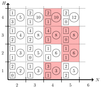
Figure 22: Directed last-passage percolation formulation of DGCG. The independent random variables $W_{N,H}$ and $U_{N,H}$ are written in rectangular boxes in each cell, and the variables $L_{N,H}$ (times at which each cell is covered by the growing interface) are circled. Shaded are the cells which are covered instantaneously during the growth.

Define a family of random variables $L_{N,H}\in\mathbb{Z}_{\geq 1}$, $N\geq 2$, $H\geq 1$, depending on the $W$’s and the $U$’s via the recurrence relation

$$\begin{split}&L_{N,H}:=\max(L_{N-1,H},L_{N,H-1})+W_{N,H}\\ &\hskip 50.0pt-W_{N,H}\mathbf{1}_{L_{N-1,H}>L_{N,H-1}}\sum_{j=1}^{N-2}\mathbf{1}_{L_{N-1,H}=\ldots=L_{N-j,H}>L_{N-j-1,H}}\mathbf{1}_{U_{N-j,H}\geq j},\end{split}$$ (A.1)

together with the boundary conditions

$$L_{1,H}=L_{N,0}=0,\qquad H\geq 0,\quad N\geq 1.$$ (A.2)

An example is given in Figure 22.

Proposition A.5.

The time-dependent formulation $\{H_{T}(N)\}$ (with homogeneous parameters) and the last-passage formulation $\{L_{N,H}\}$ are equivalent in the sense that

$$L_{N,H}=\min\left\{T\colon H_{T}(N)=H\right\}$$

for all $H\geq 1$, $N\geq 2$.

Proof.

In $\{H_{T}(N)\}$ a cell $(N,H)$ in the lattice can be covered by the growing interface at the step $T\to T+1$ in two cases:

1. it was an inner corner, and event (1.2) occurred;

2. it was added to the covered inner corner instantaneously according to the probabilities (1.3)–(1.4).

Here $W_{N,H}$ is identified with the waiting time to cover $(N,H)$ once this cell becomes an inner corner. The coefficient by $W_{N,H}$ in the second line in (A.1) is the indicator of the event that the cell $(N,H)$ is covered instantaneously by a covered inner corner at some $(N-j,H)$. The random variable $U_{N-j,H}$ is precisely the random number of boxes which are instantaneously added when $(N-j,H)$ is covered, and it has to be at least $j$ to cover $(N,H)$. Moreover, it must be $L_{N-1,H}>L_{N,H-1}$, this corresponds to the truncation in (1.3). When $(N,H)$ is covered instantaneously (so that the indicator is equal to $1$), we have $L_{N,H}=L_{N-1,H}$, and $W_{N,H}$ is not added. ∎

Remark A.6.

The first line in (A.1) corresponds to the usual directed last-passage percolation model with geometric weights. Denote it by $\widetilde{L}_{N,H}$, i.e., $\widetilde{L}_{N,H}=\max(\widetilde{L}_{N-1,H},\widetilde{L}_{N,H-1})+W_{N,H}$ (with the same boundary conditions (A.2)). Almost surely we have $\widetilde{L}_{N,H}\geq L_{N,H}$ for all $N,H$. Limit shape and fluctuation results for $\widetilde{L}_{N,H}$ were obtained in [Joh00] (for the homogeneous case $a_{N}\equiv a$). In Section 6 we compare our limit shape with the one for $\widetilde{L}_{N,H}$.

A.3 Strict-weak first-passage percolation

Any TASEP with parallel update and step initial configuration can be restated in terms of the First-Passage Percolation (FPP) on a strict-weak lattice. Let us define the FPP model. Take a lattice $\{(T,j)\colon T\geq 0,\,j\geq 1\}$, and draw its elements as $(1,0)T+(1,1)j\subset\mathbb{R}^{2}$, see Figure 23. Assign random weights to the edges of the lattice: put weight zero at each diagonal edge, and independent random weights with gB distribution (Definition A.1) at all horizontal edges. This model (with the gB distributed weights) appeared in [Mar09] together with a queuing interpretation, see Remark A.8 below. Its limit shape was described in [Mar09] in terms of a Legendre dual.

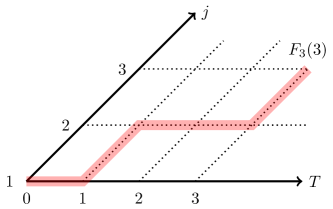
Figure 23: Interpreting $G_{j}(T)$ as first-passage percolation times.

We consider directed paths on our lattice, i.e., paths which are monotone in both $T$ and $j$. For any path, define its weight to be the sum of weights of all its edges. Let the first passage time $F_{j}(T)$ from $(0,0)$ to $(T,j)$ to be the minimal weight of a path over all directed paths from $(0,0)$ to $(T,j)$.

Proposition A.7.

We have $F_{j}(T)=G_{j}(T+j-1)+j$ for all $j,T$ (equality in distribution of families of random variables), where $G_{j}(T)$ is the coordinate of the $j$-th particle in the gB-TASEP started from the step initial configuration.

Proof.

The first passage times satisfy the recurrence:

$$F_{j}(T)=\min(F_{j-1}(T),F_{j}(T-1)+w_{j,T}),$$

where $w_{j,T}$ is the gB random variable at the horizontal edge connecting $(j,T-1)$ and $(j,T)$. At the same time, the gB-TASEP particle locations satisfy

$$G_{j}(T)=\min(G_{j-1}(T-1)-1,G_{j}(T-1)+\tilde{w}_{j,T}),$$

where $\tilde{w}_{j,T}$ is the gB random variable corresponding to the desired jump of the $j$-th particle at time step $T-1\to T$. One readily sees that the boundary conditions for these recurrences also match, which completes the proof. ∎

The FPP times $F_{j}(T)$ have an interpretation in terms of column Robinson-Schensted-Knuth (RSK) correspondence. We refer to [Ful97], [Sag01], [Sta01] for details on the RSK correspondences. Applying the column RSK to a random integer matrix of size $j\times(T+j-1)$ with independent gB entries, one gets a random Young diagram $\lambda=(\lambda_{1}\geq\ldots\geq\lambda_{j}\geq 0)$ of at most $j$ rows. The FPP time is related to this diagram as $F_{j}(T)=\lambda_{j}$. The full diagram $\lambda$ can also be recovered with the help of Greene’s theorem [Gre74] by considering minima of weights over nonintersecting directed paths in the strict-weak lattice with edge weights coming from the integer matrix.

To the best of our knowledge, the gB distribution presents a new family of random variables for which the corresponding oriented FPP times (obtained by applying the column RSK to a random matrix with independent entries) can be analyzed to the point of asymptotic fluctuations. Other known examples of random variables with tractable (to the point of asymptotic fluctuations) behavior of the FPP times consist of the pure geometric and Bernoulli distributions. Under a Poisson degeneration, the question of oriented FPP fluctuations can be reduced to the Ulam’s problem on asymptotics of the longest increasing subsequence in a random permutation. Tracy-Widom fluctuations in the latter case were obtained in the celebrated work [BDJ99].

Remark A.8.

The oriented FPP model (as well as the TASEP with parallel update) is equivalent to a tandem queuing system. For our models, the service times in the queues have the gB distribution. We refer to [Bar01], [O’C03], [Mar09] for tandem queue interpretation of the usual TASEP as well as of the column RSK correspondence. See also the end of Section 1.6 for a similar interpretation of the continuous space TASEP.

A.4 Continuous space TASEP and semi-discrete directed percolation

The homogeneous version (i.e., with $\xi(\chi)\equiv 1$) of the continuous space TASEP with no roadblocks possesses an interpretation in the spirit of directed First-Passage Percolation (FPP). This construction is very similar to a well-known interpretation of the usual continuous time TASEP on $\mathbb{Z}$ via FPP. We are grateful to Jon Warren for this observation.

Fix $M\in\mathbb{Z}_{\geq 1}$ and consider the space $\mathbb{R}_{\geq 0}\times\{1,\ldots,M\}$ in which each copy of $\mathbb{R}_{\geq 0}$ is equipped with an independent standard Poisson point process of rate $1$. See Figure 24 for an illustration. Let us first recall the connection to the usual continuous time, discrete space TASEP $(\tilde{X}_{1}(t)>\tilde{X}_{2}(t)>\ldots)$, $\tilde{X}_{i}(t)\in\mathbb{Z}$, $t\in\mathbb{R}_{\geq 0}$, started from the step initial configuration $\tilde{X}_{i}(0)=-i$, $i=1,2,\ldots$. In this TASEP each particle has an independent exponential clock with rate $1$, and when the clock rings it jumps to the right by one provided that the destination is unoccupied.

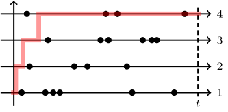
Figure 24: A minimal energy up-right path from $(0,1)$ to $(t,4)$ in the semi-discrete Poisson environment. We have $\tilde{X}_{4}(t)+4=3$.

Fix $t\in\mathbb{R}_{>0}$. For each $m=1,\ldots,M$ consider up-right paths from $(0,1)$ to $(t,m)$ as in Figure 24. The energy of an up-right path is, by definition, the total number of points in the Poisson processes lying on this path.

Proposition A.9.

For each $m$ and $t$, the minimal energy of an up-right path from $(0,1)$ to $(t,m)$ in the Poisson environment has the same distribution as the displacement $\tilde{X}_{m}(t)+m$ of the $m$-th particle in the usual TASEP.

For the continuous space TASEP consider a variant of this construction by putting an independent exponential random weight with mean $L^{-1}$ at each point of each of the Poisson processes as in Figure 24. That is, let now the weight of each point be random instead of $1$. One can say that we replace the Poisson processes on $\mathbb{R}_{\geq 0}\times\left\{1,\ldots,M\right\}$ by marked Poisson processes. This environment corresponds to the continuous space TASEP $(X_{1}(t)\geq X_{2}(t)\geq\ldots)$, $X_{i}(t)\in\mathbb{R}_{\geq 0}$:

Proposition A.10.

For each $t>0$ and $m=1,\ldots,M$ the minimal energy of an up-right path from $(0,1)$ to $(t,m)$ in the marked Poisson environment has the same distribution as the coordinate $X_{m}(t)$ of the $m$-th particle in the continuous space TASEP with mean jumping distance $L^{-1}$.

Both Propositions A.9 and A.10 are established similarly to Proposition A.7 while taking into account the continuous horizontal coordinate. The interpretation via minimal energies of up-right paths also allows to define random Young diagrams depending on the Poisson or marked Poisson processes, respectively, by minimizing over collections of nonintersecting up-right paths. Utilizing Greene’s theorem [Gre74], (see also [Ful97], [Sag01], or [Sta01]) one sees that in the case of the usual TASEP the distribution of this Young diagram is the Schur measure $\propto s_{\lambda}(1,\ldots,1)s_{\lambda}(\vec{0};\vec{0};t)$. It would be very interesting to understand the distribution and asymptotics of random Young diagrams arising from the marked Poisson environment.

Appendix B Hydrodynamic equations for limiting densities

Here we present informal derivations of hydrodynamic partial differential equations which the limiting densities and height functions of the DGCG and continuous space TASEP should satisfy. These equations follow from constructing families of local translation invariant stationary distributions of arbitrary density for the corresponding dynamics. The argument could be made rigorous if one shows that these families exhaust all possible (nontrivial) translation invariant stationary distributions (as, e.g., it is for TASEP [Lig05] or PushTASEP [Gui97], [AG05]). We do not pursue this classification question here.

B.1 Hydrodynamic equation for DGCG

Consider the discrete DGCG model in the asymptotic regime described in Section 6. Locally around every scaled point $\eta$ the distribution of the process should be translation invariant and stationary under the homogeneous version of DGCG on $\mathbb{Z}$ (recall that it depends on the three parameters $a,\beta,\nu$). The existence (for suitable initial configurations) of the homogeneous dynamics on $\mathbb{Z}$ can be established similarly to [Lig73], [And82].

A supply of translation invariant stationary distributions on particle configurations on $\mathbb{Z}$ is given by product measures. That is, let us independently put particles at each site of $\mathbb{Z}$ with the gB probability (cf. Definition A.1)

$$\pi(j):=\mathop{\mathrm{Prob}}(\textnormal{$j$ particles at a site})=\begin{cases}\displaystyle\frac{1-c}{1-c\nu},&j=0;\\[10.0pt] \displaystyle c^{j}\,\frac{(1-c)(1-\nu)}{1-c\nu},&j\geq 1.\end{cases}$$ (B.1)

Proposition B.1.

The product measure $\pi^{\otimes\mathbb{Z}}$ on particle configurations in $\mathbb{Z}$ corresponding to the distribution $\pi$ (B.1) at each site is invariant under the homogeneous DGCG on $\mathbb{Z}$ with any values of the parameters $a$ and $\beta$.

Proof.

Let us check directly that $\pi$ is invariant, i.e., satisfies

$$\pi(k+1)P(k+1\to k)+\pi(k-1)P(k-1\to k)+\pi(k)P(k\to k)=\pi(k),\qquad k=0,1,2,\ldots,$$ (B.2)

where $P(k\to l)$ are the one-step transition probabilities of the homogeneous DGCG restricted to a given site (say, we are looking at site $0$). The probability that a particle coming from the left crosses the bond $-1\to 0$ is equal to

$$u:=\sum_{n=0}^{\infty}\pi(0)^{n}(1-\pi(0))\frac{a\beta}{1+a\beta}\left(\frac{\nu+a\beta}{1+a\beta}\right)^{n}=\frac{ac\beta}{1+ac\beta},$$

where we sum over the number of empty sites to the left of $0$, multiply by the probability that a particle leaves a stack, and then travels distance $n$. We have

$$P(k+1\to k)=\frac{a\beta}{1+a\beta}(1-u),$$

the probability that a particle leaves the stack at $0$, and another particle does not join it from the left. Moreover, for $k\geq 1$ we have

$$P(k-1\to k)=\frac{u(1-\nu)}{1+a\beta}\,\mathbf{1}_{k=1}+\frac{u}{1+a\beta}\,\mathbf{1}_{k\geq 2},$$

where for $k=1$ we require that the moving particle stops at site $0$, and for $k\geq 2$ we need the stack at $0$ not to emit a particle. Finally,

$$P(k\to k)=\left(1-\frac{u(1-\nu)}{1+a\beta}\right)\mathbf{1}_{k=0}+\left(\frac{a\beta u}{1+a\beta}+\frac{1-u}{1+a\beta}\right)\mathbf{1}_{k\geq 1},$$

where we require that no particle has stopped at site $0$ for $k=0$ and sum over two possibilities to preserve the number of particles at $0$ for $k\geq 1$. With these probabilities written down, checking (B.2) is straightforward. ∎

The density of particles under the product measure $\pi^{\otimes\mathbb{Z}}$ is $\rho(c)=\frac{c(1-\nu)}{(1-c)(1-c\nu)}$, and the current (i.e., the average number of particles crossing a given bond) is equal to the quantity $u$ from the proof of Proposition B.1, that is, $j(c)=\frac{ca\beta}{1+ca\beta}$. Thus, the dependence of the current on the density has the form (where we recall that the parameters $a,\nu$ depend on the space coordinate $\eta$)

$$j(\rho)=\frac{2a\beta\rho}{2a\beta\rho+\nu(\rho-1)+\rho+1+\sqrt{(\nu(\rho-1)+\rho+1)^{2}-4\nu\rho^{2}}}.$$ (B.3)

The partial differential equation for the limiting density $\rho(\tau,\eta)$ expressing the continuity of the hydrodynamic flow has the form [AK84], [Rez91], [Lan96], [GKS10]

$$\frac{\partial}{\partial\tau}\rho(\tau,\eta)+\frac{\partial}{\partial\eta}j\bigl{(}\rho(\tau,\eta)\bigr{)}=0.$$ (B.4)

One can readily verify that the limit shape (6.1) satisfies this equation. Equation (B.4) should also hold for the scaling limit of the inhomogeneous DGCG, when the parameters $a,\beta,\nu$ of the homogeneous dynamics on the full line $\mathbb{Z}$ depend on the spatial coordinate $\eta$. That is, one should replace $j(\rho(\tau,\eta))$ (B.3) by $j(\rho(\tau,\eta);\eta)$ with $a=a(\eta),a=\beta(\eta),a=\nu(\eta)$ being the scaled values of the parameters.

B.2 Hydrodynamic equation for continuous space TASEP

Assume that the set of roadblocks $\mathbf{B}$ is empty. Then locally at every point $\chi>0$ the behavior of the continuous space TASEP should be homogeneous. Locally the parameters can be chosen so that the mean waiting time to jump is $1/\xi\equiv 1/\xi(\chi)$ and the mean jumping distance is $1$.

The local distribution (on the full line $\mathbb{R}$) should be invariant under space translations, and stationary under our homogeneous Markov dynamics. The existence (for suitable initial configurations) of the dynamics on $\mathbb{R}$ can be established similarly to [Lig73], [And82].

A supply of translation invariant stationary distributions of arbitrary density may be constructed as follows. Fix a parameter $0<c<1$ and consider a Poisson process on $\mathbb{R}$ with rate (i.e., mean density) $\frac{c}{1-c}$. Put a random geometric number of particles at each point of this Poisson process, independently at each point, with the geometric distribution

$$\mathrm{Prob}(\textnormal{$j\geq 1$ particles})=(1-c)c^{j-1}.$$

Thus we obtain a so-called marked Poisson process — a distribution of stacks of particles on $\mathbb{R}$. It is clearly translation invariant. The stationarity of this process under the dynamics (for any $\xi$) follows by setting $q=0$ in [BP18a, Appendix B] so we omit the computation here.

The density of particles under this marked Poisson process is

$$\rho=\frac{c}{(1-c)^{2}}.$$

One can check that the current of particles (that is, the mean number of particles passing through, say, zero, in a unit of time) has the form

$$j=\xi c=\xi\,\frac{1+2\rho-\sqrt{1+4\rho}}{2\rho}.$$

The partial differential equation for the limiting density $\rho(\theta,\chi)$ (under the scaling described in Section 4.1) expressing the continuity of the hydrodynamic flow has the form $\rho_{\theta}+(j(\rho))_{\chi}=0$, or

$$\frac{\partial}{\partial\theta}\rho(\theta,\chi)+\frac{\partial}{\partial\chi}\biggl{[}\xi(\chi)\,\frac{1+2\rho(\theta,\chi)-\sqrt{1+4\rho(\theta,\chi)}}{2\rho(\theta,\chi)}\biggr{]}=0,\qquad\rho(0,\chi)=+\infty\,\mathbf{1}_{\chi=0}.$$ (B.5)

The density is related to the limiting height function as $\rho(\theta,\chi)=-\frac{\partial}{\partial\chi}\mathfrak{h}(\theta,\chi)$, and so $\mathfrak{h}$ should satisfy

$$\mathfrak{h}_{\chi}(\theta,\chi)=-\frac{\xi(\chi)\mathfrak{h}_{\theta}(\theta,\chi)}{\bigl{(}\xi(\chi)-\mathfrak{h}_{\theta}(\theta,\chi)\bigr{)}^{2}},\qquad\mathfrak{h}(0,\chi)=+\infty\,\mathbf{1}_{\chi=0}.$$ (B.6)

The passage from (B.5) to (B.6) is done via integrating from $\chi$ to $+\infty$ followed by algebraic manipulations. One can check that the limit shape in the curved part

$$\mathfrak{h}(\theta,\chi)=\theta\mkern 2.0mu\mathfrak{w}^{\circ}(\theta,\chi)-\int\limits_{0}^{\chi}\dfrac{\xi(u)\mathfrak{w}^{\circ}(\theta,\chi)du}{(\xi(u)-\mathfrak{w}^{\circ}(\theta,\chi))^{2}}$$

from Definition 4.3 indeed satisfies (B.6) whenever all derivatives make sense. Such a check is very similar to the one performed in the discrete case in Section B.1 (and also corresponds to setting $q=0$ in [BP18a, Appendix B]), so we omit it for the continuous model.

Appendix C Fluctuation kernels

C.1 Airy₂ kernel and GUE Tracy-Widom distribution

Let $\mathsf{Ai}(x):=\frac{1}{2\pi}\int e^{i\sigma^{3}/3+i\sigma x}d\sigma$ be the Airy function, where the integration is over a contour in the complex plane from $e^{{\mathbf{i}\mkern 1.0mu}\frac{5\pi}{6}}\infty$ through $0$ to $e^{{\mathbf{i}\mkern 1.0mu}\frac{\pi}{6}}\infty$. Define the extended Airy kernel [Mac94], [FNH99], [PS02] on $\mathbb{R}\times\mathbb{R}$ by

$$\begin{split}&\mathsf{A}^{\mathrm{ext}}(s,x;s^{\prime},x^{\prime})=\begin{cases}\int_{0}^{\infty}e^{-\mu(s-s^{\prime})}\mathsf{Ai}(x+\mu)\mathsf{Ai}(x^{\prime}+\mu)d\mu,&\mbox{if $s\geq s^{\prime}$};\\ -\int_{-\infty}^{0}e^{-\mu(s-s^{\prime})}\mathsf{Ai}(x+\mu)\mathsf{Ai}(x^{\prime}+\mu)d\mu,&\mbox{if $s<s^{\prime}$}\end{cases}\\[4.0pt] &\hskip 10.0pt=-\frac{\mathbf{1}_{s<s^{\prime}}}{\sqrt{4\pi(s^{\prime}-s)}}\exp\left(-\frac{(x-x^{\prime})^{2}}{4(s^{\prime}-s)}-\frac{1}{2}(s^{\prime}-s)(x+x^{\prime})+\frac{1}{12}(s^{\prime}-s)^{3}\right)\\ &\hskip 30.0pt+\frac{1}{(2\pi{\mathbf{i}\mkern 1.0mu})^{2}}\iint\exp\Big{(}sx-s^{\prime}x^{\prime}-\frac{1}{3}s^{3}+\frac{1}{3}s^{\prime 3}-(x-s^{2})u+(x^{\prime}-s^{\prime 2})v\\ &\hskip 160.0pt-su^{2}+s^{\prime}v^{2}+\frac{1}{3}(u^{3}-v^{3})\Big{)}\frac{du\,dv}{u-v}.\end{split}$$ (C.1)

In the double contour integral expression, the $v$ integration contour goes from $e^{-{\mathbf{i}\mkern 1.0mu}\frac{2\pi}{3}}\infty$ through $0$ to $e^{{\mathbf{i}\mkern 1.0mu}\frac{2\pi}{3}}\infty$, and the $u$ contour goes from $e^{-{\mathbf{i}\mkern 1.0mu}\frac{\pi}{3}}\infty$ through $0$ to $e^{{\mathbf{i}\mkern 1.0mu}\frac{\pi}{3}}\infty$, and the integration contours do not intersect. This expression for the extended Airy kernel which is most suitable for our needs appeared in [BK08, Section 4.6], see also [Joh03].

We also use the following gauge transformation of the extended Airy kernel:

$$\begin{split}&\widetilde{\mathsf{A}}^{\mathrm{ext}}(s,x;s^{\prime},x^{\prime}):=e^{-sx+s^{\prime}x^{\prime}+\frac{1}{3}s^{3}-\frac{1}{3}s^{\prime 3}}\mathsf{A}^{\mathrm{ext}}(s,x;s^{\prime},x^{\prime})\\ &\hskip 20.0pt=-\frac{\mathbf{1}_{s<s^{\prime}}}{\sqrt{4\pi(s^{\prime}-s)}}\exp\left(-\frac{(s^{2}-x-s^{\prime 2}+x^{\prime})^{2}}{4(s^{\prime}-s)}\right)\\ &\hskip 40.0pt+\frac{1}{(2\pi{\mathbf{i}\mkern 1.0mu})^{2}}\iint\exp\Big{(}-(x-s^{2})u+(x^{\prime}-s^{\prime 2})v-su^{2}+s^{\prime}v^{2}+\frac{1}{3}(u^{3}-v^{3})\Big{)}\frac{du\,dv}{u-v}.\end{split}$$ (C.2)

When $s=s^{\prime}$, $\mathsf{A}^{\mathrm{ext}}(s,x;s^{\prime},x^{\prime})$ becomes the usual Airy kernel (independent of $s$):

$$\begin{split}\mathsf{A}(x;x^{\prime}):=\mathsf{A}^{\mathrm{ext}}(s,x;s,x^{\prime})&=\frac{1}{(2\pi{\mathbf{i}\mkern 1.0mu})^{2}}\iint\frac{e^{u^{3}/3-v^{3}/3-xu+x^{\prime}v}du\,dv}{u-v}\\ &=\frac{\mathsf{Ai}(x)\mathsf{Ai}^{\prime}(x^{\prime})-\mathsf{Ai}^{\prime}(x)\mathsf{Ai}(x^{\prime})}{x-x^{\prime}},\hskip 45.0ptx,x^{\prime}\in\mathbb{R}.\end{split}$$ (C.3)

The GUE Tracy-Widom distribution function [TW94] is the following Fredholm determinant of (C.3):

$$F_{GUE}(r)=\det\left(\mathbf{1}-\mathsf{A}\right)_{(r,+\infty)},\qquad r\in\mathbb{R},$$ (C.4)

defined analogously to (3.15) with sums replaced by integrals over $(r,+\infty)$.

C.2 BBP deformation of the Airy₂ kernel

Fix $m$ and a vector $\mathbf{b}=(b_{1},\ldots,b_{m})\in\mathbb{R}^{m}$. Define the extended BBP kernel on $\mathbb{R}\times\mathbb{R}$ by

$$\begin{split}&\widetilde{\mathsf{B}}^{\mathrm{ext}}_{m,\mathbf{b}}(s,x;s^{\prime},x^{\prime}):=-\frac{\mathbf{1}_{s<s^{\prime}}}{\sqrt{4\pi(s^{\prime}-s)}}\exp\left(-\frac{(s^{2}-x-s^{\prime 2}+x^{\prime})^{2}}{4(s^{\prime}-s)}\right)\\ &\hskip 10.0pt+\frac{1}{(2\pi{\mathbf{i}\mkern 1.0mu})^{2}}\iint\prod_{j=1}^{m}\frac{v-b_{i}}{u-b_{i}}\exp\Big{(}-(x-s^{2})u+(x^{\prime}-s^{\prime 2})v-su^{2}+s^{\prime}v^{2}+\frac{1}{3}(u^{3}-v^{3})\Big{)}\frac{du\,dv}{u-v}.\end{split}$$ (C.5)

The integration contours are as in the Airy kernel (C.1) with the additional condition that they both must pass to the left of the poles $b_{i}$.

For $s=s^{\prime}=0$ this kernel (denote it by $\widetilde{\mathsf{B}}_{m,\mathbf{b}}(x,x^{\prime})$) was introduced in [BBP05] the context of spiked random matrices. The extended version appeared in [IS07]. In this paper we are using the gauge transformation similar to (C.2), hence the tilde in the notation. Denote for $\mathbf{b}=(0,\ldots,0)$ the corresponding distribution function by

$$F_{m}(r):=\det\bigl{(}\mathbf{1}-\widetilde{\mathsf{B}}_{m,\mathbf{b}}\bigr{)}_{(r,+\infty)},\qquad r\in\mathbb{R}.$$

Remark C.1.

Note that in several other papers, e.g., [BCF14], [Bar15], [BP18a] the kernel like (C.5) has the reversed product $\prod_{i=1}^{m}\frac{u-b_{i}}{v-b_{i}}$, but the contours pass to the right of the poles. Such a form is equivalent to (C.5). In [BP08] a common generalization with poles on both sides of the contours is considered.

C.3 Deformation of the Airy₂ kernel arising at a traffic jam

For $\delta>0$ introduce the following deformation of the extended Airy₂ kernel (C.2):

$$\begin{split}&\widetilde{\mathsf{A}}^{\mathrm{ext,\delta}}(s,x;s^{\prime},x^{\prime})=-\frac{\mathbf{1}_{s<s^{\prime}}}{\sqrt{4\pi(s^{\prime}-s)}}\exp\left(-\frac{(s^{2}-x-s^{\prime 2}+x^{\prime})^{2}}{4(s^{\prime}-s)}\right)\\ &\hskip 20.0pt+\frac{1}{(2\pi{\mathbf{i}\mkern 1.0mu})^{2}}\iint\exp\bigg{(}\frac{\delta}{v}-\frac{\delta}{u}-(x-s^{2})u+(x^{\prime}-s^{\prime 2})v-su^{2}+s^{\prime}v^{2}+\frac{1}{3}(u^{3}-v^{3})\bigg{)}\frac{du\,dv}{u-v}\end{split}$$ (C.6)

with the same integration contours as in the Airy kernel with the additional condition that they both pass to the left of $0$. This kernel can be related to certain random matrix and percolation models considered in [BP08], see Section 5.5.4 for details. A Fredholm determinant at $s=s^{\prime}$ of this kernel is a deformation of the GUE Tracy-Widom distribution (C.4):

$$F_{GUE}^{(\delta,s)}(r)=\det\bigl{(}\mathbf{1}-\widetilde{\mathsf{A}}^{\mathrm{ext},\delta}(s,\cdot;s,\cdot)\bigr{)}_{(r,+\infty)},\qquad r\in\mathbb{R}.$$ (C.7)

Note that this deformation additionally depends on $s$ in contrast with the undeformed case, so the deformation breaks translation invariance of the kernel and the process. When $\delta=0$, both the extended kernel (C.6) and the deformed Tracy-Widom GUE distribution turn into the corresponding undeformed objects.

One can show by a change of variables in the integral in (C.6) that $F_{GUE}^{(\delta,0)}(r+2\delta^{\frac{1}{2}})\to F_{GUE}(2^{-\frac{2}{3}}r)$ as $\delta\to+\infty$. This explains why the deformed distribution $F_{GUE}^{(\delta,0)}$ arises at a phase transition between two GUE Tracy-Widom laws. We are grateful to Guillaume Barraquand for this observation.

C.4 Fluctuation kernel in the Gaussian phase

Let $m\in\mathbb{Z}_{\geq 1}$ and $\gamma>0$ be fixed. Define the kernel on $\mathbb{R}$ as follows:

$$\begin{split}\widetilde{\mathsf{G}}^{\mathrm{ext}}_{m,\gamma}(h;h^{\prime})&:=-\mathbf{1}_{\gamma>1}\frac{\exp\left\{-\frac{(h-h^{\prime}\gamma)^{2}}{2(\gamma^{2}-1)}\right\}}{\sqrt{2\pi(\gamma^{2}-1)}}\\ &\hskip 50.0pt+\frac{1}{(2\pi{\mathbf{i}\mkern 1.0mu})^{2}}\iint\exp\left\{-\tfrac{1}{2}w^{2}+\tfrac{1}{2}z^{2}-hw+h^{\prime}z\right\}\left(\frac{z}{w\gamma}\right)^{m}\frac{dz\,dw}{z-w\gamma}.\end{split}$$ (C.8)

The $z$ contour is a vertical line in the left half-plane traversed upwards which crosses the real line to the left of $-\gamma$. The $w$ contour goes from $e^{-{\mathbf{i}\mkern 1.0mu}\frac{\pi}{6}}\infty$ to $-1$ to $e^{{\mathbf{i}\mkern 1.0mu}\frac{\pi}{6}}$.

For $\gamma=1$ a Fredholm determinant of this kernel describes the distribution of the largest eigenvalue of an $m\times m$ GUE random matrix $H=[H_{ij}]_{i,j=1}^{m}$, $H^{*}=H$, $\mathop{\mathrm{Re}}H_{ij}\sim\mathcal{N}\bigl{(}0,\frac{1+\mathbf{1}_{i=j}}{2}\bigr{)}$, $i\geq j$, $\mathop{\mathrm{Im}}H_{ij}\sim\mathcal{N}\bigl{(}0,\frac{1}{2}\bigr{)}$, $i>j$. That is, the distribution function of the largest eigenvalue is

$$G_{m}(r)=\det\bigl{(}\mathbf{1}-\widetilde{\mathsf{G}}_{m,1}^{\mathrm{ext}}\bigr{)}_{(r,+\infty)}.$$

The extended version (C.8) appeared in [EM98], [IS05] (see also [IS07]).

Acknowledgments.

We are grateful to Guillaume Barraquand, Riddhipratim Basu, Alexei Borodin, Eric Cator, Francis Comets, Ivan Corwin, Patrik Ferrari, Vadim Gorin, Pavel Krapivsky, Alexander Povolotsky, Timo Seppäläinen, and Jon Warren for helpful discussions. A part of the work was completed when the authors attended the 2017 IAS PCMI Summer Session on Random Matrices, and we are grateful to the organizers for the hospitality and support. AK was partially supported by the NSF grant DMS-1704186. LP was partially supported by the NSF grant DMS-1664617.

A. Knizel, Department of Mathematics, Columbia University

E-mail address: knizel@math.columbia.edu

L. Petrov, Department of Mathematics, University of Virginia, and Institute for Information Transmission Problems

E-mail address: lenia.petrov@gmail.com

A. Saenz, Department of Mathematics, University of Virginia

E-mail address: ais6a@virginia.edu

References

- [Agg18] A. Aggarwal “Current Fluctuations of the Stationary ASEP and Six-Vertex Model” arXiv:1608.04726 [math.PR] In Duke Math J. 167.2, 2018, pp. 269–384
- [And82] E. Andjel “Invariant measures for the zero range process” In Ann. Probab. 10.3, 1982, pp. 525–547
- [AG05] E. Andjel and H. Guiol “Long-range exclusion processes, generator and invariant measures” arXiv:math/0411655 [math.PR] In Ann. Probab. 33.6, 2005, pp. 2314–2354
- [AK84] E. Andjel and C. Kipnis “Derivation of the hydrodynamical equation for the zero-range interaction process” In Ann. Probab. 12.2 Institute of Mathematical Statistics, 1984, pp. 325–334
- [Bai06] J. Baik “Painlevé formulas of the limiting distributions for nonnull complex sample covariance matrices” arXiv:math/0504606 [math.PR] In Duke Math J. 133.2, 2006, pp. 205–235
- [BBP05] J. Baik, G. Ben Arous and S. Péché “Phase transition of the largest eigenvalue for nonnull complex sample covariance matrices” arXiv:math/0403022 [math.PR] In Ann. Probab. 33.5, 2005, pp. 1643–1697
- [BDJ99] J. Baik, P. Deift and K. Johansson “On the distribution of the length of the longest increasing subsequence of random permutations” arXiv:math/9810105 [math.CO] In Jour. AMS 12.4 American Mathematical Society, 1999, pp. 1119–1178
- [BKS12] M. Balász, J. Komjáthy and T. Seppäläinen “Microscopic concavity and fluctuation bounds in a class of deposition processes” In Ann. Inst. H. Poincaré B 48, 2012, pp. 151–187
- [Bar15] G. Barraquand “A phase transition for q-TASEP with a few slower particles” arXiv:1404.7409 [math.PR] In Stochastic Processes and their Applications 125.7, 2015, pp. 2674–2699
- [Bar01] Yu. Baryshnikov “GUEs and queues” In Probab. Theory Relat. Fields 119, 2001, pp. 256–274
- [BSS17] R. Basu, S. Sarkar and A. Sly “Invariant Measures for TASEP with a Slow Bond” arXiv:1704.07799 In arXiv preprint, 2017
- [BSS14] R. Basu, V. Sidoravicius and A. Sly “Last Passage Percolation with a Defect Line and the Solution of the Slow Bond Problem” arXiv:1408.3464 [math.PR] In arXiv preprint, 2014
- [BNKR94] E. Ben-Naim, P. Krapivsky and S. Redner “Kinetics of clustering in traffic flows” arXiv:cond-mat/9402054 In Phys. Rev. E. 50.2 APS, 1994, pp. 822–829
- [Ben+99] M. Bengrine, A. Benyoussef, H. Ez-Zahraouy, J. Krug, M. Loulidi and F. Mhirech “A simulation study of an asymmetric exclusion model with disorder” In MJ Condensed Matter 2.1, 1999, pp. 117–126
- [Bla11] M. Blank “Exclusion-type spatially heterogeneous processes in continua” arXiv:1105.4232 [math.DS] In Jour. Stat. Mech. 2011.06, 2011, pp. P06016
- [Bla12] M. Blank “Discrete Time TASEP in Heterogeneous Continuum” In Markov Processes and Related Fields 18.3, 2012, pp. 531–552
- [Bor10] Folkmar Bornemann “On the numerical evaluation of Fredholm determinants” arXiv:0804.2543 [math.NA] In Math. Comp. 79.270, 2010, pp. 871–915
- [Bor11] A. Borodin “Determinantal point processes” arXiv:0911.1153 [math.PR] In Oxford Handbook of Random Matrix Theory Oxford University Press, 2011
- [Bor17] A. Borodin “On a family of symmetric rational functions” arXiv:1410.0976 [math.CO] In Adv. Math. 306, 2017, pp. 973–1018 eprint: 1410.0976
- [BC14] A. Borodin and I. Corwin “Macdonald processes” arXiv:1111.4408 [math.PR] In Probab. Theory Relat. Fields 158, 2014, pp. 225–400
- [BCF14] A. Borodin, I. Corwin and P. Ferrari “Free energy fluctuations for directed polymers in random media in 1+ 1 dimension” arXiv:1204.1024 [math.PR] In Comm. Pure Appl. Math. 67.7, 2014, pp. 1129–1214
- [BD11] A. Borodin and M. Duits “Limits of determinantal processes near a tacnode” arXiv:0911.1980 [math.PR] In Annales de l’institut Henri Poincaré (B) 47.1, 2011, pp. 243–258
- [BF14] A. Borodin and P. Ferrari “Anisotropic growth of random surfaces in 2+1 dimensions” arXiv:0804.3035 [math-ph] In Commun. Math. Phys. 325, 2014, pp. 603–684
- [BFPS07] A. Borodin, P. Ferrari, M. Prähofer and T. Sasamoto “Fluctuation properties of the TASEP with periodic initial configuration” arXiv:math-ph/0608056 In J. Stat. Phys. 129.5-6, 2007, pp. 1055–1080
- [BFS09] A. Borodin, P. Ferrari and T. Sasamoto “Two speed TASEP” arXiv:0904.4655 [math-ph] In J. Stat. Phys 137.5, 2009, pp. 936–977
- [BK08] A. Borodin and J. Kuan “Asymptotics of Plancherel measures for the infinite-dimensional unitary group” arXiv:0712.1848 [math.RT] In Adv. Math. 219.3, 2008, pp. 894–931
- [BOO00] A. Borodin, A. Okounkov and G. Olshanski “Asymptotics of Plancherel measures for symmetric groups” arXiv:math/9905032 [math.CO] In Jour. AMS 13.3, 2000, pp. 481–515 eprint: math/9905032
- [BO07] A. Borodin and G. Olshanski “Asymptotics of Plancherel-type random partitions” arXiv:math/0610240 In Journal of Algebra 313.1 Elsevier, 2007, pp. 40–60
- [BO16] A. Borodin and G. Olshanski “Representations of the Infinite Symmetric Group” Cambridge University Press, 2016
- [BO17] A. Borodin and G. Olshanski “The ASEP and determinantal point processes” arXiv:1608.01564 [math-ph] In Comm. Math. Phys 353.2, 2017, pp. 853–903
- [BP08] A. Borodin and S. Peche “Airy kernel with two sets of parameters in directed percolation and random matrix theory” arXiv:0712.1086v3 [math-ph] In Jour. Stat. Phys. 132.2, 2008, pp. 275–290
- [BP16] A. Borodin and L. Petrov “Lectures on Integrable probability: Stochastic vertex models and symmetric functions” arXiv:1605.01349 [math.PR] In Lecture Notes of the Les Houches Summer School 104, 2016 eprint: 1605.01349
- [BP16a] A. Borodin and L. Petrov “Nearest neighbor Markov dynamics on Macdonald processes” arXiv:1305.5501 [math.PR] In Adv. Math. 300, 2016, pp. 71–155 eprint: 1305.5501
- [BP18] A. Borodin and L. Petrov “Higher spin six vertex model and symmetric rational functions” arXiv:1601.05770 [math.PR] In Selecta Math. 24.2, 2018, pp. 751–874 eprint: 1601.05770
- [BP18a] A. Borodin and L. Petrov “Inhomogeneous exponential jump model” arXiv:1703.03857 [math.PR] In Probab. Theory Relat. Fields 172, 2018, pp. 323–385 eprint: 1703.03857
- [BM18] A. Bufetov and K. Matveev “Hall-Littlewood RSK field” arXiv:1705.07169 [math.PR] In Selecta Math. 24.5, 2018, pp. 4839–4884
- [BP17] A. Bufetov and L. Petrov “Yang-Baxter field for spin Hall-Littlewood symmetric functions” arXiv:1712.04584 [math.PR] In arXiv preprint, 2017 eprint: 1712.04584
- [Cal15] J. Calder “Directed last passage percolation with discontinuous weights” In Jour. Stat. Phys. 158.4, 2015, pp. 903–949
- [CG18] F. Ciech and N. Georgiou “Last passage percolation in an exponential environment with discontinuous rates” arXiv:1808.00917 [math.PR] In arXiv preprint, 2018
- [CEP96] Henry Cohn, Noam Elkies and James Propp “Local statistics for random domino tilings of the Aztec diamond” arXiv:math/0008243 [math.CO] In Duke Math. J. 85.1, 1996, pp. 117–166 DOI: 10.1215/S0012-7094-96-08506-3
- [Cor12] I. Corwin “The Kardar-Parisi-Zhang equation and universality class” arXiv:1106.1596 [math.PR] In Random Matrices Theory Appl. 1, 2012
- [Cor16] I. Corwin “Kardar-Parisi-Zhang Universality” In Notices of the AMS 63.3, 2016, pp. 230–239
- [CP16] I. Corwin and L. Petrov “Stochastic higher spin vertex models on the line” arXiv:1502.07374 [math.PR] In Commun. Math. Phys. 343.2, 2016, pp. 651–700 eprint: 1502.07374
- [CT18] I. Corwin and L.-C. Tsai “SPDE Limit of Weakly Inhomogeneous ASEP” arXiv:1806.09682 [math.PR] In arXiv preprint, 2018
- [CLST13] O. Costin, J. Lebowitz, E. Speer and A. Troiani “The blockage problem” arXiv:1207.6555 [math-ph] In Bull. Inst. Math. Acad. Sinica (New Series) 8.1, 2013, pp. 47–72
- [DPPP12] A. Derbyshev, S. Poghosyan, A. Povolotsky and V. Priezzhev “The totally asymmetric exclusion process with generalized update” arXiv:1203.0902 [cond-mat.stat-mech] In Jour. Stat. Mech. IOP Publishing, 2012
- [DPP15] A. Derbyshev, A. Povolotsky and V. Priezzhev “Emergence of jams in the generalized totally asymmetric simple exclusion process” arXiv:1410.2874 [math-ph] In Physical Review E 91.2, 2015, pp. 022125
- [DLSS91] B. Derrida, J. Lebowitz, E. Speer and H. Spohn “Dynamics of an anchored Toom interface” In J. Phys. A 24.20, 1991, pp. 4805
- [DW08] A.B. Dieker and J. Warren “Determinantal transition kernels for some interacting particles on the line” arXiv:0707.1843 [math.PR] In Annales de l’Institut Henri Poincaré 44.6, 2008, pp. 1162–1172 Institut Henri Poincaré
- [DZS08] J. Dong, R. Zia and B. Schmittmann “Understanding the edge effect in TASEP with mean-field theoretic approaches” arXiv:0809.1974 [cond-mat.stat-mech] In Journal of Physics A 42.1, 2008, pp. 015002
- [Dui13] M. Duits “The Gaussian free field in an interlacing particle system with two jump rates” arXiv:1105.4656 [math-ph] In Comm. Pure Appl. Math. 66.4, 2013, pp. 600–643
- [Edr52] A. Edrei “On the generating functions of totally positive sequences. II” In J. Analyse Math. 2, 1952, pp. 104–109
- [Emr16] E. Emrah “Limit shapes for inhomogeneous corner growth models with exponential and geometric weights” arXiv:1502.06986 [math.PR] In Electron. Commun. Probab. 21.42, 2016, pp. 16
- [Erd53] “Higher transcendental functions” McGraw–Hill, 1953
- [EM98] B. Eynard and M.L. Mehta “Matrices coupled in a chain: I. Eigenvalue correlations” In J. Phys. A 31 IOP Publishing, 1998, pp. 4449–4456
- [Fer08] P. Ferrari “The universal Airy1 and Airy2 processes in the Totally Asymmetric Simple Exclusion Process” arXiv:math-ph/0701021 In Integrable Systems and Random Matrices: In Honor of Percy Deift, Contemporary Math. AMS, 2008, pp. 321–332
- [FS11] P. Ferrari and H. Spohn “Random Growth Models” arXiv:1003.0881 [math.PR] In Oxford Handbook of Random Matrix Theory Oxford University Press, 2011
- [FNH99] P.J. Forrester, T. Nagao and G. Honner “Correlations for the orthogonal-unitary and symplectic-unitary transitions at the hard and soft edges” arXiv:cond-mat/9811142 [cond-mat.mes-hall] In Nuclear Physics B 553.3, 1999, pp. 601–643
- [Ful97] W. Fulton “Young Tableaux with Applications to Representation Theory and Geometry” Cambridge University Press, 1997
- [GKS10] N. Georgiou, R. Kumar and T. Seppäläinen “TASEP with discontinuous jump rates” arXiv:1003.3218 [math.PR] In ALEA Lat. Am. J. Probab. Math. Stat. 7, 2010, pp. 293–318
- [GTW02] J. Gravner, C. Tracy and H. Widom “Fluctuations in the composite regime of a disordered growth model” In Commun. Math. Phys. 229, 2002, pp. 433–458
- [Gre74] C. Greene “An extension of Schensted’s theorem” In Adv. Math. 14.2, 1974, pp. 254–265
- [Gui97] H. Guiol “Un résultat pour le processus d’exclusion à longue portée [A result for the long-range exclusion process]” In Annales de l’Institut Henri Poincare (B) Probability and Statistics 33.4, 1997, pp. 387–405
- [HHT15] T. Halpin-Healy and K. Takeuchi “A KPZ cocktail-shaken, not stirred…” arXiv:1505.01910 [cond-mat.stat-mech] In J. Stat. Phys 160.4 Springer, 2015, pp. 794–814
- [Hel01] D. Helbing “Traffic and related self-driven many-particle systems” arXiv:cond-mat/0012229 [cond-mat.stat-mech] In Reviews of modern physics 73.4 APS, 2001, pp. 1067–1141
- [HKPV06] J.B. Hough, M. Krishnapur, Y. Peres and B. Virág “Determinantal processes and independence” arXiv:math/0503110 [math.PR] In Probability Surveys 3, 2006, pp. 206–229
- [IS05] T. Imamura and T. Sasamoto “Polynuclear growth model with external source and random matrix model with deterministic source” In Phys. Rev. E. 71.4 APS, 2005, pp. 041606
- [IS07] T. Imamura and T. Sasamoto “Dynamics of a tagged particle in the asymmetric exclusion process with the step initial condition” arXiv:math-ph/0702009 In Jour. Stat. Phys. 128.4 Springer, 2007, pp. 799–846
- [ITW01] A. Its, C. Tracy and H. Widom “Random words, Toeplitz determinants and integrable systems” In Random Matrices and Their Applications 40, MSRI Publications, 2001
- [JL92] S. Janowsky and J. Lebowitz “Finite-size effects and shock fluctuations in the asymmetric simple-exclusion process” In Physical Review A 45.2, 1992, pp. 618
- [JPS98] W. Jockusch, J. Propp and P. Shor “Random domino tilings and the arctic circle theorem” arXiv:math/9801068 [math.CO] In arXiv preprint, 1998
- [Joh00] K. Johansson “Shape fluctuations and random matrices” arXiv:math/9903134 [math.CO] In Commun. Math. Phys. 209.2 Springer, 2000, pp. 437–476
- [Joh03] K. Johansson “Discrete polynuclear growth and determinantal processes” arXiv:math/0206208 [math.PR] In Commun. Math. Phys. 242.1, 2003, pp. 277–329
- [Joh16] K. Johansson “Two time distribution in Brownian directed percolation” arXiv:1502.00941 [math-ph] In Commun. Math. Phys., 2016, pp. 1–52 DOI: 10.1007/s00220-016-2660-5
- [Joh18] K. Johansson “The two-time distribution in geometric last-passage percolation” arXiv:1802.00729 [math.PR] In arXiv preprint, 2018
- [Kru91] J. Krug “Boundary-induced phase transitions in driven diffusive systems” In Phys. Rev. Lett. 67.14 APS, 1991, pp. 1882–1885
- [Kru00] J. Krug “Phase separation in disordered exclusion models” arXiv:cond-mat/9912411 [cond-mat.stat-mech] In Brazilian Journal of Physics 30.1, 2000, pp. 97–104
- [KF96] J. Krug and P.A. Ferrari “Phase transitions in driven diffusive systems with random rates” In Journal of Physics A: Mathematical and General 29.18, 1996, pp. L465
- [Lan96] C. Landim “Hydrodynamical limit for space inhomogeneous one-dimensional totally asymmetric zero-range processes” In Ann. Probab. 24.2, 1996, pp. 599–638
- [Lig73] T. Liggett “An infinite particle system with zero range interactions” In Ann. Probab. 1.2, 1973, pp. 240–253
- [Lig76] T. Liggett “Coupling the simple exclusion process” In Ann. Probab., 1976, pp. 339–356
- [Lig99] T. Liggett “Stochastic Interacting Systems: Contact, Voter and Exclusion Processes” 324, Grundlehren de mathematischen Wissenschaften Springer, 1999
- [Lig05] T. Liggett “Interacting Particle Systems” Berlin: Springer-Verlag, 2005
- [MGP68] C. MacDonald, J. Gibbs and A. Pipkin “Kinetics of biopolymerization on nucleic acid templates” In Biopolymers 6.1, 1968, pp. 1–25
- [Mac95] I.G. Macdonald “Symmetric functions and Hall polynomials” Oxford University Press, 1995
- [Mac94] A. M. S. Macêdo “Universal parametric correlations at the soft edge of the spectrum of random matrix ensembles” arXiv:cond-mat/9404038 In Europhys. Lett. 26.9, 1994, pp. 641
- [Mar09] J. Martin “Batch queues, reversibility and first-passage percolation” arXiv:0902.2026 [math.PR] In Queueing Systems 62.4, 2009, pp. 411–427
- [MQR17] K. Matetski, J. Quastel and D. Remenik “The KPZ fixed point” arXiv:1701.00018 [math.PR] In arXiv preprint, 2017
- [O’C03] N. O’Connell “A path-transformation for random walks and the Robinson-Schensted correspondence” In Trans. AMS 355.9, 2003, pp. 3669–3697
- [O’C03a] N. O’Connell “Conditioned random walks and the RSK correspondence” In J. Phys. A 36.12, 2003, pp. 3049–3066
- [OP13] N. O’Connell and Y. Pei “A q-weighted version of the Robinson-Schensted algorithm” arXiv:1212.6716 [math.CO] In Electron. J. Probab. 18.95, 2013, pp. 1–25
- [Oko01] A. Okounkov “Infinite wedge and random partitions” arXiv:math/9907127 [math.RT] In Selecta Math. 7.1 Springer, 2001, pp. 57–81
- [OR03] A. Okounkov and N. Reshetikhin “Correlation function of Schur process with application to local geometry of a random 3-dimensional Young diagram” arXiv:math/0107056 [math.CO] In Jour. AMS 16.3 American Mathematical Society, 2003, pp. 581–603
- [OP17] D. Orr and L. Petrov “Stochastic Higher Spin Six Vertex Model and -TASEPs” In Adv. Math. 317, 2017, pp. 473–525 DOI: 10.1016/j.aim.2017.07.003
- [Pet19] L. Petrov “PushTASEP in inhomogeneous space” In preparation, 2019
- [Pov13] A. Povolotsky “On integrability of zero-range chipping models with factorized steady state” arXiv:1308.3250 [math-ph] In J. Phys. A 46, 2013, pp. 465205
- [PS02] M. Prähofer and H. Spohn “Scale invariance of the PNG droplet and the Airy process” arXiv:math.PR/0105240 In J. Stat. Phys. 108, 2002, pp. 1071–1106
- [QS15] J. Quastel and H. Spohn “The one-dimensional KPZ equation and its universality class” arXiv:1503.06185 [math-ph] In J. Stat. Phys 160.4, 2015, pp. 965–984
- [Rez91] F. Rezakhanlou “Hydrodynamic limit for attractive particle systems on ” In Commun. Math. Phys. 140.3 Springer, 1991, pp. 417–448
- [RT08] L. Rolla and A. Teixeira “Last passage percolation in macroscopically inhomogeneous media” In Electron. Commun. Probab. 13, 2008, pp. 131–139
- [Ros81] H. Rost “Nonequilibrium behaviour of a many particle process: density profile and local equilibria” In Z. Wahrsch. Verw. Gebiete 58.1, 1981, pp. 41–53 URL: https://doi.org/10.1007/BF00536194
- [Sag01] B.E. Sagan “The symmetric group: representations, combinatorial algorithms, and symmetric functions” Springer Verlag, 2001
- [Sep98] T. Seppäläinen “Hydrodynamic scaling, convex duality and asymptotic shapes of growth models” In Markov Process. Related Fields 4.1, 1998, pp. 1–26
- [Sep99] T. Seppäläinen “Existence of hydrodynamics for the totally asymmetric simple K-exclusion process” In Ann. Probab. 27.1, 1999, pp. 361–415
- [Sep01] T. Seppäläinen “Hydrodynamic profiles for the totally asymmetric exclusion process with a slow bond” arXiv:math/0003049 [math.PR] In J. Stat. Phys 102.1-2, 2001, pp. 69–96
- [SK99] T. Seppäläinen and J. Krug “Hydrodynamics and platoon formation for a totally asymmetric exclusion model with particlewise disorder” In Jour. Stat. Phys. 95.3-4 Springer, 1999, pp. 525–567
- [Sim05] B. Simon “Trace ideals and their applications, second edition” 120, Mathematical Surveys and Monographs AMS, 2005
- [Sos00] A. Soshnikov “Determinantal random point fields” arXiv:math/0002099 [math.PR] In Russian Mathematical Surveys 55.5, 2000, pp. 923–975
- [Spi70] F. Spitzer “Interaction of Markov processes” In Adv. Math. 5.2, 1970, pp. 246–290
- [Spo91] H. Spohn “Large scale dynamics of interacting particles” Springer, 1991
- [Sta01] R. Stanley “Enumerative Combinatorics. Vol. 2” With a foreword by Gian-Carlo Rota and appendix 1 by Sergey Fomin Cambridge: Cambridge University Press, 2001
- [Tho64] E. Thoma “Die unzerlegbaren, positive-definiten Klassenfunktionen der abzählbar unendlichen, symmetrischen Gruppe” In Math. Zeitschr 85, 1964, pp. 40–61
- [TTCB10] AG Thompson, J Tailleur, ME Cates and RA Blythe “Zero-range processes with saturated condensation: the steady state and dynamics” arXiv:0912.3009 [cond-mat.stat-mech] In Jour. Stat. Mech., 2010, pp. P02013
- [TW94] C. Tracy and H. Widom “Level-spacing distributions and the Airy kernel” arXiv:hep-th/9211141 In Commun. Math. Phys. 159.1 Springer, 1994, pp. 151–174
- [TW09] C. Tracy and H. Widom “Asymptotics in ASEP with step initial condition” arXiv:0807.1713 [math.PR] In Commun. Math. Phys. 290, 2009, pp. 129–154
- [WW09] J. Warren and P. Windridge “Some examples of dynamics for Gelfand-Tsetlin patterns” arXiv:0812.0022 [math.PR] In Electron. J. Probab. 14 The Institute of Mathematical Statisticsthe Bernoulli Society, 2009, pp. 1745–1769
- [Woe05] M. Woelki “Steady states of discrete mass transport models”, 2005
- [ZDS11] R.K.P. Zia, J.J. Dong and B. Schmittmann “Modeling Translation in Protein Synthesis with TASEP: A Tutorial and Recent Developments” In J. Stat. Phys 144.405, 2011 DOI: s10955-011-0183-1