Gaussian quantum fluctuations in the superfluid-Mott phase transition

Abstract

Recent advances in cooling techniques make now possible the experimental study of quantum phase transitions, which are transitions near absolute zero temperature accessed by varying a control parameter. A paradigmatic example is the superfluid-Mott transition of interacting bosons on a periodic lattice. From the relativistic Ginzburg-Landau action of this superfluid-Mott transition we derive the elementary excitations of the bosonic system, which contain in the superfluid phase a gapped Higgs mode and a gappless Goldstone mode. We show that this energy spectrum is in good agreement with the available experimental data and we use it to extract, with the help of dimensional regularization, meaningful analytical formulas for the beyond-mean-field equation of state in two and three spatial dimensions. We find that, while the mean-field equation of state always gives a second-order quantum phase transition, the inclusion of Gaussian quantum fluctuations can induce a first-order quantum phase transition. This prediction is a strong benchmark for next future experiments on quantum phase transitions.

The Bose-Hubbard model of interacting bosons on a periodic lattice was introduced in 1963 by Gersch and Knollman Gersch to describe the coherent properties of granular superconductors. The model gained much success by the late 1980s Ma ; Giamarchi ; Fisher . More recently it has been used to investigate superconductivity and ultracold atoms in optical lattices Bruder ; Sachdev , but also quantum information Romero and quantum chaos Kolowsky . The bosonic gas described the Bose-Hubbard model displays a quantum phase transition between a superfluid phase and the Mott insulating phase Ma ; Giamarchi ; Fisher ; Sachdev ; Greiner ; Kacz . This transition corresponds to a global $U(1)$ spontaneous symmetry breaking Goldstone ; Higgs ; Varma ; Altland . The spectrum of the Mott phase shows two gapped modes, whereas the superfluid phase has a gapless Goldstone mode and a gapped mode, which in condensed matter physics is called Higgs mode Varma . These features have been recently observed experimentally Endres . However, an experimental investigation of the equation of state around the superfluid-Mott phase quantum transition is still missing.

Near the superfluid-Mott transition the Bose-Hubbard model can be mapped into an low-energy and low-momenta effective action India ; Stoof ; Dupuis ; kennett . This action is a generalization of the familiar high-temperature Ginzburg-Landau functional Ginzburg and it contains also time derivatives of the order parameter. These additional terms, which make the action formally relativistic, are indeed crucial at low temperature. This kind of effective action has been recently used to study the Higgs mode in the BCS-BEC crossover with s-wave fermion superfluids BLiu .

In this work, we adopt this effective relativistic Ginzburg-Landau action and, within a functional interation formalism Altland , we compute the elementary excitations which are in good agreement with experimental results Endres and share formal analogies with the ones of both the non-relativistic and relativistic weakly interacting gases. Furthermore, in order to compute the equation of state, we regularize divergent integrals by using dimensional regularization t'Hooft ; Capper ; Salasnich-Toigo . In this way we find that, within our beyond-mean-field Gaussian scheme, the superfluid-Mott phase transition changes from second order to first order due to quantum fluctuations. Only at the critical points the quantum phase transition remains of the second order.

Historically, the phenomenon of a first-order transition induced by quantum fluctuations was suggested by Coleman and Weinberg Coleman studying a massless charged meson coupled to the electrodynamic field, and by Halperin, Lubensky, and Ma Halperin investigating the fluctuations of the electromagnetic field in the superconductor to normal metal transition. More recently, this phenomenon has been theoretically predicted also for other other phase transitions. For instance, the ferromagnet-helix transition in an isotropic quantum Heisenberg ferromagnet Rastelli , the ferromagnetic-paramagnetic transition in local Fermi liquid Bedell , and the superfluid-Mott transition at the critical points for a two-species bosonic system in a three-dimensional optical lattice Liu . In this paper we are proposing a much more sophisticated effect: the Gaussian quantum fluctuations of a single $U(1)$ order parameter can trigger a quantum phase transition from second- to first-order, without the coupling to other dynamical fields. Quite remarkably, our theoretical results for the zero-temperature equation of state can be directly tested with the experimental setups Greiner ; Endres of ultracold alkali-metal atoms loaded into three-dimensional or quasi two-dimensional optical lattices.

I Mean-field phase diagram and effective action

The Bose-Hubbard Hamiltonian is given by

$$\hat{H}=-J\sum_{\langle ij\rangle}\hat{a}_{i}^{\dagger}\hat{a}_{j}+{U\over 2}\sum_{i}\hat{n}_{i}(\hat{n}_{i}-1)-(\mu-\epsilon)\sum_{i}\hat{n}_{i}\;,$$ (1)

where $\hat{a}_{i}$ is the bosonic annihilation operator at the site $i$, $\hat{n}_{i}={\hat{a}}^{+}_{i}{\hat{a}}_{i}$ is the corresponding bosonic number operator, $\epsilon$ is the on-site energy of bosons, $\mu$ is the chemical potential, $J$ is the hopping term, which describes the tunneling energy of particles, and $U$ is the on-site interaction strength of bosons.

Within the mean-field decopling approximation Sachdev the boundary between the superfluid phase and the Mott phase in the Bose-Hubbard model are obtained from the equation

$$(\mu-\epsilon)^{2}-(\mu-\epsilon)\left(U(2n-1)-2DJ\right)$$

$$+2DJU+U^{2}n(n-1)=0\;.$$ (2)

In Fig. 1 we plot the superfluid-Mott phase diagram of the Bose-Hubbard model at zero temperature, obtained from Eq. (2). Inside the lobes there is the Mott phase, characterized by an integer filling number $n$ and where the expectation value of the annihilation operator for each site is equal to zero. Outside the Mott lobes there is the superfluid phase, characterized by a non-vanishing expectation value of the annihilation operator for each site. The tips of the lobes are critical points. The corresponding critical transitions, which occur for $n=1$ at $[2DJ/U]_{c}=0.172$ and $[(\mu-\epsilon)/U]_{c}=0.414$, can be controlled by varying $U$ at fixed $J$ or varying $J$ at fixed $U$. Non-critical transitions, which are the ones not occurring at the tips, can be instead obtained, at fixed $J$ and $U$, by changing the effective chemical potential $\mu-\epsilon$.

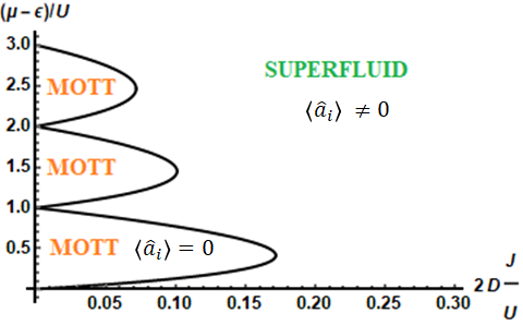
Figure 1: Mean-field phase diagram of the Bose-Hubbard model at zero temperature in $D$ spatial dimensions. $J$ is the hopping energy, $\epsilon$ is the on-site energy, $U$ is the on-site interaction energy, $\mu$ is the chemical potential. The tips of the Mott lobes are critical points.

In the vicinity of the transition line, the Bose-Hubbard model can be mapped into the following effective Ginzburg-Landau action in Euclidean space India ; Stoof ; Dupuis

$$S = \beta\mathcal{E}_{0}+\int_{0}^{\beta}d\tau\,\int_{V}d^{D}\vec{r}\,\Big{\{}K_{1}\psi^{*}\frac{\partial}{\partial\tau}\psi+K_{2}\left|\frac{\partial}{\partial\tau}\psi\right|^{2}$$ (3)

$$+ K_{3}|\vec{\nabla}\psi|^{2}+c_{2}|\psi|^{2}+c_{4}|\psi|^{4}\Big{\}}\;,$$

where $\psi({\vec{x}},\tau)=\langle{\hat{a}}_{i}(\tau)\rangle$ is the space-time dependent order parameter, which corresponds to the expectation value of the annihilation operator ${\hat{a}}_{i}(\tau)$ at the imaginary time $\tau$ and at the site $i$ associated to spatial position ${\vec{x}}$. Here $\beta=1/T$ with $T$ the absolute temperature, $V$ is the volume, and

$$\mathcal{E}_{0}=V\left(-(\mu-\epsilon)n+{U\over 2}n(n-1)\right)$$ (4)

is the mean-field energy of the bosonic system in the Mott phase, with $n$ the integer filling number of the Mott lobe. The parameters $K_{1}$, $K_{2}$, $K_{3}$, $c_{2}$, and $c_{4}$ of the effective action (3) can be expressed in terms of the Bose-Hubbard parameters $J$, $U$, and $\mu-\epsilon$, and the condition $c_{2}=0$ is equivalent to Eq. (2). We stress that $c_{4}$, $K_{2}$ and $K_{3}$ are always positive, while $K_{1}$ vanishes for transitions at the critical points (i.e. tips of the lobes). See Appendix 1 for details.

The effective action (3) is a generalization of the Ginzburg-Landau functional Ginzburg and the term which contains $K_{2}$ makes the action formally relativistic. In general, the time-dependent terms are very important for an accurate description of the bosonic system at low temperature. We shall show that the quantum fluctuations extracted from the effective action (3) crucially depend on $K_{1}$ and $K_{2}$ and strongly affect the zero-temperature equation of state. In the spirit of the Ginzburg-Landau approach, $K_{1}$, $K_{2}$, $K_{3}$ and $c_{4}$ are calculated at the chosen transition point, while $c_{2}$ remains the only quantity that is tuned by the selected control parameter across the transition point.

II Partition function and elementary excitations

By using the path integral formalism Altland , the partition function of the bosonic system near the superfluid-Mott transition is then given by

$$Z=\int\,D[\psi,\psi^{*}]\ \exp\{-S[\psi,\psi^{*}]\}\;.$$ (5)

From the partition function we can compute the grand-canonical potential as

$$\Omega=-\frac{1}{\beta}\ln(Z)\;.$$ (6)

Since our system is homogeneous, the pressure is simply given by $P=-\Omega/V$. We write the order parameter as

$$\psi({\vec{x}},\tau)=\psi_{0}+\eta({\vec{x}},\tau)\;,$$ (7)

where $\psi_{0}$ is the uniform and constant order parameter and $\eta({\vec{x}},\tau)$ takes into account space-time fluctuations around $\psi_{0}$. In this way, the grand-canonical potential can be written as

$$\Omega=\Omega^{(MF)}+\Omega^{(G)}\;,$$ (8)

where $\Omega^{(MF)}$ is the mean-field grand potential associated $\psi_{0}$ while $\Omega^{(G)}$ is associated to the fluctuating field $\eta({\vec{x}},\tau)$ at the Gaussian level.

From Eqs. (3), (6) and (7), the mean-field contribution reads

$$\Omega^{(MF)}={\cal E}_{0}+V\ \left(c_{2}\ |\psi_{0}|^{2}+c_{4}\ |\psi_{0}|^{4}\right)\;.$$ (9)

By minimizing this grand potential we obtain, assuming $\psi_{0}$ real,

$$\psi_{0}=\left\{\begin{array}[]{ll}0&\mbox{ if }c_{2}>0\\ \sqrt{|c_{2}|\over 2c_{4}}&\mbox{ if }c_{2}<0\end{array}\right.$$ (10)

Thus, the mean-field grand-canonical potential becomes

$$\Omega^{(MF)}=\mathcal{E}_{0}-V\frac{c_{2}^{2}}{c_{4}}\Theta(-c_{2})\;,$$ (11)

where $\Theta(x)$ is the Heaviside step function. We remind that the phase diagram shown in Fig. 1 is obtained within this mean-field picture.

The zero-temperature Gaussian grand potential is instead given by the zero-point energy Altland ; Salasnich-Toigo

$$\Omega^{(G)}={1\over 2}\sum_{\vec{q}}\sum_{j=1,2}E_{\vec{q},j}\;,$$ (12)

where $E_{\vec{q},j}$ are the elementary excitations characterized by two branches ($j=1,2$). Here $E_{\vec{q},j}=\omega_{j}(\vec{q})$, where the frequencies $\omega_{j}(\vec{q})$ are derived from $\mbox{det}[{\cal M}({\bf q},\omega)]=0$. The $4\times 4$ matrix ${\cal M}(\vec{q},i\Omega_{m})$ is the inverse propagator of Gaussian fluctuations with $\vec{q}$ the $D$-dimensional wavevector, $\Omega_{m}=2\pi m/\beta$ the Matsubara frequencies, and $i=\sqrt{-1}$ the imaginary unit. See Faccioli-Salasnich for details on the derivation of ${\cal M}(\vec{q},i\Omega_{m})$ in the case of both non-relativistic and relativistic bosonic actions.

Inside the Mott phase ($c_{2}>0$) the energy spectrum reads

$$E_{\vec{q},j}=\sqrt{\frac{K_{3}}{K_{2}}q^{2}+\left(\frac{K_{1}^{2}}{4K_{2}^{2}}+\frac{c_{2}}{K_{2}}\right)}+(-1)^{j}\frac{|K_{1}|}{2K_{2}}\;,$$ (13)

whereas for the superfluid phase ($c_{2}<0$) we have

$$E_{\vec{q},j}^{2} = \frac{K_{3}}{K_{2}}q^{2}+\left(\frac{K_{1}^{2}}{2K_{2}^{2}}-\frac{c_{2}}{K_{2}}\right)$$ (14)

$$+ (-1)^{j}\sqrt{\frac{K_{1}^{2}K_{3}}{K_{2}^{3}}q^{2}+\left(\frac{K_{1}^{2}}{2K_{2}^{2}}-\frac{c_{2}}{K_{2}}\right)^{2}}\;.$$

We observe that both modes in the Mott phase are gapped, whereas in the superfluid phase we have a gapped (Higgs) mode and a gapless (Goldstone) one as expected by Goldstone theorem. Clearly, for $K_{1}=0$ the gapless mode is linear, namely

$$E_{\vec{q},1}=\sqrt{K_{3}\over K_{2}}\ q\;.$$ (15)

For $K_{1}\neq 0$ the small-momentum expansion is a bit more involved but one finds that the gapless mode is still linear at small momentum, i.e.

$$E_{\vec{q},1}\simeq\sqrt{{K_{3}\over K_{2}}-{K_{1}^{2}K_{3}\over 2K_{2}^{3}(\frac{K_{1}^{2}}{2K_{2}^{2}}-\frac{c_{2}}{K_{2}})}}\ q\;.$$ (16)

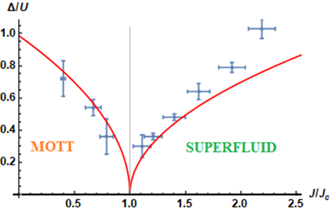
Figure 2: We compare the predictions of our theory (solid line) for the sum $\Delta$ of the two gaps with experimental data (squares with error bars) of Ref. Endres . In the horizontal axis $J_{c}$ is the critical value of $J$ at which the critical transition of the $n=1$ Mott lobe occurs. Within our theoretical scheme $J_{c}$ is given by $J_{c}=0.043\ U$.

We show in Fig. 2 a comparison between the predictions of our theory for the sum of the two gaps

$$\Delta=E_{\vec{q}=\vec{0},1}+E_{\vec{q}=\vec{0},2}\;,$$ (17)

and the available experimental data Endres . These data are obtained with ultracold and dilute bosonic atoms loaded into a quasi two-dimensional optical lattice, studying the superfluid-Mott transition at the critical point ($K_{1}=0$) of the $n=1$ lobe. In the experiment the on-site interaction strength $U$ was fixed and the hopping energy $J$ was changed. The figure shows that the gaps of our elementary excitations above the uniform and constant order parameter are in quite good agreement with experimental data for the Mott phase, and also with the results in the superfluid phase close to the transition line. Notice that, in the superfluid phase within our Gaussian approach we get

$$\Delta=E_{\vec{q}=\vec{0},2}=\sqrt{2}\sqrt{\frac{K_{1}^{2}}{2K_{2}^{2}}-\frac{c_{2}}{K_{2}}}\;,$$ (18)

while in the Mott phase we obtain

$$E_{\vec{q}=\vec{0},j}=\sqrt{\frac{K_{1}^{2}}{4K_{2}^{2}}+\frac{c_{2}}{K_{2}}}+(-1)^{j}\frac{|K_{1}|}{2K_{2}}\;.$$ (19)

When the linear time derivative is absent ($K_{1}=0$), at the critical transition ($c_{2}=0$) all the gaps vanish. We stress that our results are also consistent with other theoretical approaches to the elementary excitations of the two-dimensional Bose-Hubbard model Altman ; Huber .

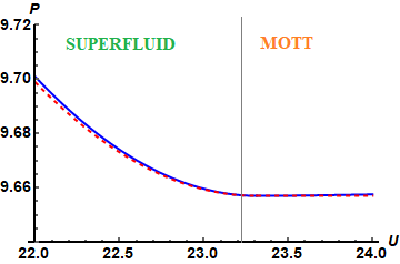
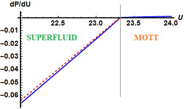
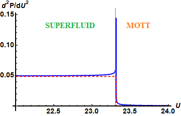
Figure 3: Pressure $P=-\Omega/V$ and its derivatives with respect to the control parameter $U$, across the critical point (tip) of the $n=1$ Mott lobe, as a function of $U$. Red dashed line: mean-field theory. Blue solid line: beyond-mean-field theory. Results obtained for the two-dimensional bosonic system, with $J=1$ and $[(\mu-\epsilon)/U]_{c}=0.414$.

III Beyond mean-field equation of state

We now compute the beyond mean-field equation of state. First of all, we consider the case with a vanishing linear time derivative of the order parameter ($K_{1}=0$). We have seen that this very special case corresponds to a transition across the critical points (tips of the Mott lobes). In this case, the Gaussian correction to the mean-field grand-canonical potential reads

$$\Omega^{(G)}=\frac{1}{1+\Theta(-c_{2})}\sum_{j=1,2}\sum_{\vec{q}}\sqrt{K_{3}q^{2}+|c_{2}|+(-1)^{j}|c_{2}|\Theta(-c_{2})}\;.$$ (20)

After performing the continuum limit in the sum over momenta and the dimensional regularization of the divergent integrals (see Appendix 2 for details), the beyond-mean-field grand-canonical potential, that is the zero-temperature equation of state, for $D=2$ reads

$$\Omega=\mathcal{E}_{0}-V\frac{c_{2}^{2}}{c_{4}}\Theta(-c_{2})-V\frac{|c_{2}|^{3/2}}{3\pi K_{3}}\frac{1}{\sqrt{1+\Theta(-c_{2})}}\;,$$ (21)

while for $D=3$ it is given by

$$\Omega = \mathcal{E}_{0}-V\frac{c_{2}^{2}}{c_{4}}\Theta(-c_{2})-V\frac{c_{2}^{2}}{16\pi^{2}K_{3}^{3/2}}$$ (22)

$$\cdot \Big{[}\ln\left(\frac{q_{0}K_{3}^{1/2}}{|c_{2}|^{1/2}}\right)+\frac{3}{4}-\frac{\gamma}{2}\Big{]}[1+\Theta(-c_{2})]\;,$$

where $\gamma=0.577$ is the Eulero-Mascheroni constant and $q_{0}$ is an ultraviolet cut-off in the momenta, related to the maximal length scale of the system.

In Fig. 3 we report our predictions for the pressure $P=-\Omega/V$ in the case of a critical transition ($K_{1}=0$). In the figure we consider a two-dimensional system ($D=2$) and the superfluid-Mott transition at the tip of the $n=1$ Mott lobe. We plot the pressure $P$ as a function of the control parameter $U$. Fig. 3 shows that the first-order derivative of the pressure with the respect to $U$ is continuous. Instead, the second-order derivative of the pressure with the respect to $U$ has a divergence at the transition. Remarkably, this case with $D=2$ is analogous to what is found for the specific heat of a $D=3$ system in the classical Ginzburg-Landau theory Kardar . In the case $D=3$ we find similar results. Thus, at the critical points, the superfluid-Mott phase transition is of the second order both in $D=2$ and $D=3$, and the Gaussian quantum fluctuations do not change the order of the transition.

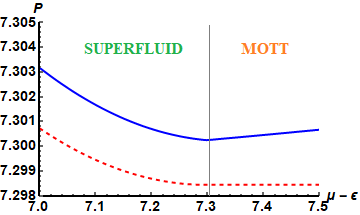
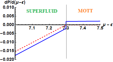
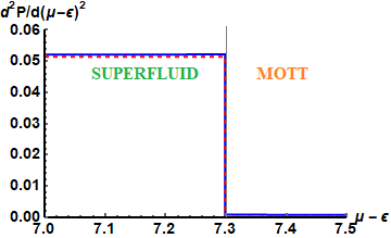
Figure 4: Pressure $P=-\Omega/V$ and its derivatives with respect to the control parameter $\mu-\epsilon$, across a non-critical transition point of the $n=1$ Mott lobe, as a function of $\mu-\epsilon$. Red dashed line: mean-field theory. Blue solid line: beyond-mean-field theory. Results obtained for the two-dimensional bosonic system, with $J=1$ and $U=25$.

Including the linear time derivative of the order parameter ($K_{1}\neq 0$) the situation changes dramatically. In particular we find that for $D=2$ the equation of state reads

$$\Omega=\mathcal{E}_{0}-V\frac{c_{2}^{2}}{c_{4}}\Theta(-c_{2})-V\frac{\left(\frac{K_{1}^{2}}{4K_{2}}+|c_{2}|\right)^{\frac{3}{2}}}{6\pi K_{3}}\;,$$ (23)

while for $D=3$ the grand-canonical potential is given by

$$\Omega = \mathcal{E}_{0}-V\frac{c_{2}^{2}}{c_{4}}\Theta(-c_{2})-V\frac{\Big{(}\frac{K_{1}^{2}}{4K_{2}}+|c_{2}|\Big{)}^{2}}{16\pi^{2}K_{3}^{\frac{3}{2}}}$$ (24)

$$\cdot \left\{\ln\left[\ \frac{q_{0}K_{3}^{\frac{1}{2}}}{\left(\frac{K_{1}^{2}}{4K_{2}}+|c_{2}|\right)}\right]+\frac{3}{4}-\frac{\gamma}{2}\right\}\;.$$

In both cases, we have that the first-order derivative with the respect to the control parameter $\mu-\epsilon$ has a jump discontinuity. Hence, in contrast to the second-order phase transition predicted by the mean-field we have a prediction, with the inclusion of the quantum fluctuations, of a first-order phase transition. These effects are clearly shown in Fig. 4, where we plot the behavior of the pressure $P=-\Omega/V$ and its derivatives in the case of a non critical transition. In the figure we consider again a two-dimensional bosonic system ($D=2$) and the superfluid-Mott transition across a non critical point of the $n=1$ Mott lobe. Here the chosen control parameter is $\mu-\epsilon$ and the derivatives of the pressure $P$ are calculated with respect to it, at fixed hopping $J$ and on-site interaction strength $U$.

In conclusion, Gaussian quantum fluctuations strongly modify the properties of the grand-canonical potential (or equivalently the pressure) near the superfluid-Mott transition. For critical transitions at the tips of the Mott lobes, we find a divergent second-order derivative, which is analogous to what is found for the specific heat in the classical Ginzburg-Landau theory. In all the other non-critical transition points, after including the beyond-mean-field Gaussian correction a finite discontinuity appears in the first derivative, which corresponds to a first-order phase transition. Thus, Gaussian quantum fluctuations of the order parameter itself have a crucial role on the order of the quantum phase transition. Our calculations are based on the Bose-Hubbard model but they are valid, at the Gaussian level, for any quantum phase transition described by a Ginzburg-Landau action which contains both non-relativistic and relativistic time-dependent terms.

Appendix 1. Parameters of the effective action

The parameters of the effective relativistic action (3) can be written in terms of the Bose-Hubbard parameters as Dupuis

$$c_{2} = \frac{[Un-(\mu-\epsilon)][(\mu-\epsilon)-U(n-1)]}{[(\mu-\epsilon)+U]}$$ (25)

$$- \frac{2DJ[(\mu+\epsilon)+U]}{[(\mu-\epsilon)+U]}\;,$$

$$K_{1} = -{\partial c_{2}\over\partial(\mu-\epsilon)}\;,$$ (26)

$$K_{2} = -{1\over 2}{\partial^{2}c_{2}\over\partial(\mu-\epsilon)^{2}}\;,$$ (27)

$$K_{3} = J\;,$$ (28)

where $n$ is the integer filling number, which characterizes the lobes of the Mott phase. The quartic coefficient is instead given by

$$G^{4}c_{4} = \frac{(n+1)(n+2)}{(2(\mu-\epsilon)-(2n+1)U)(Un-(\mu-\epsilon))^{2}}$$ (29)

$$+ \frac{n(n-1)}{((\mu-\epsilon)-U(n-1))^{2}(U(2n-3)-2(\mu-\epsilon))}$$

$$- \frac{n(n+1)}{((\mu-\epsilon)-Un)(-(\mu-\epsilon)+U(n-1))^{2}}$$

$$- \frac{n(n+1)}{((\mu-\epsilon)-Un)^{2}(-(\mu-\epsilon)+U(n-1))}$$

$$- \frac{n^{2}_{0}}{(-(\mu-\epsilon)+U(n-1))^{3}}-\frac{(n+1)^{2}}{((\mu-\epsilon)-Un)^{3}}\;,$$

where

$$G=\frac{n+1}{[(\mu-\epsilon)-Un]}-\frac{n}{[(\mu-\epsilon)-U(n-1)]}\;.$$ (30)

Appendix 2. Dimensional regularization

In order to find a finite expression for the beyond-mean-field grand potential we adopt the dimensional regularization technique t'Hooft ; Capper ; Salasnich-Toigo . Here we perform the dimensional regularization for $D=2$ and $D=3$, when both the linear and quadratic time derivatives are present, i.e. the case $K_{1}\neq 0$ and $K_{2}\neq 0$. The other cases are very similar. First of all, we make the continuum limit in the sum over momenta

$$\Omega^{(G)} = \sum_{\vec{q}}\sqrt{K_{3}q^{2}+\left(\frac{K_{1}^{2}}{4K_{2}}+|c_{2}|\right)}$$ (31)

$$= \frac{V}{(2\pi)^{D}}\int\,d^{D}\vec{q}\,\sqrt{K_{3}q^{2}+\left(\frac{K_{1}^{2}}{4K_{2}}+|c_{2}|\right)}\;.$$

We now write the integral in the polar coordinates

$$\Omega^{(G)}=\frac{2V}{(4\pi)^{\frac{D}{2}}\Gamma(\frac{D}{2})}\int_{0}^{\infty}\,dq\,\sqrt{K_{3}q^{2}+\left(\frac{K_{1}^{2}}{4K_{2}}+|c_{2}|\right)}\;,$$ (32)

where $\Gamma(x)$ is the Euler gamma function. After the transformation

$$Q=\frac{K_{3}}{\left(\frac{K_{1}^{2}}{4K_{2}}+|c_{2}|\right)}q^{2}$$ (33)

we get

$$\Omega^{(G)}=V\frac{\left(\frac{K_{1}^{2}}{4K_{2}}+|c_{2}|\right)^{\frac{D+1}{2}}}{(4\pi)^{\frac{D}{2}}K_{3}^{\frac{D}{2}}\Gamma(\frac{D}{2})}\int_{0}^{\infty}\,dQ\,Q^{\frac{D}{2}-1}\sqrt{1+Q}\;.$$ (34)

In order to compute this divergent integral, we shift the dimensionality as follows

$$D\quad\rightarrow\quad D-\varepsilon\;,$$ (35)

where $\varepsilon$ is a small, complex parameter. We obtain:

$$\Omega^{(G)}=V\frac{\left(\frac{K_{1}^{2}}{4K_{2}}+|c_{2}|\right)^{\frac{D-\varepsilon+1}{2}}\kappa^{\varepsilon}}{(4\pi)^{\frac{D-\varepsilon}{2}}K_{3}^{\frac{D-\varepsilon}{2}}\Gamma(\frac{D-\varepsilon}{2})}\int_{0}^{\infty}\,dQ\,Q^{\frac{D-\varepsilon}{2}-1}\sqrt{1+Q}\;,$$ (36)

where we have introduced, for dimensional reason, a momentum scale $\kappa$. Now, the integral can be written as

$$\int_{0}^{\infty}Q^{\frac{D-\varepsilon}{2}-1}\sqrt{1+Q}=\frac{\Gamma(\frac{D-\varepsilon}{2})\Gamma(-\frac{(D+1-\varepsilon)}{2})}{\Gamma(-\frac{1}{2})}\;.$$ (37)

Hence, we obtain for the Gaussian term

$$\Omega^{(G)}=V\frac{\left(\frac{K_{1}^{2}}{4K_{2}}+|c_{2}|\right)^{\frac{D-\varepsilon+1}{2}}\kappa^{\varepsilon}}{(4\pi)^{\frac{D-\varepsilon}{2}}K_{3}^{\frac{D-\varepsilon}{2}}}\frac{\Gamma(-\frac{D}{2}-\frac{1}{2}+\frac{\varepsilon}{2})}{\Gamma(-\frac{1}{2})}\;.$$ (38)

For $D=2$, we get for $\varepsilon\rightarrow 0$

$$\Omega^{(G)}=V\frac{\left(\frac{K_{1}^{2}}{4K_{2}}+|c_{2}|\right)^{\frac{3}{2}}}{6\pi K_{3}}\;.$$ (39)

For $D=3$, after regularization we still find a divergent result, because the Gamma function has poles for negative integers. To isolate the divergence, we expand the Gamma function around $\varepsilon=0$

$$\Gamma\left(-2+\frac{\varepsilon}{2}\right)=\frac{1}{\epsilon}-\frac{\gamma}{2}+\frac{3}{4}+O(\varepsilon)\;,$$ (40)

and we get

$$\frac{\left(\frac{K_{1}^{2}}{4K_{2}}+|c_{2}|\right)^{\frac{4-\varepsilon}{2}}\kappa^{\varepsilon}}{(4\pi)^{\frac{1-\varepsilon}{2}}K_{3}^{\frac{1-\varepsilon}{2}}}\frac{\Gamma(-1+\frac{\varepsilon}{2})}{\Gamma(-\frac{1}{2})}=\frac{\left(\frac{K_{1}^{2}}{4K_{2}}+|c_{2}|\right)^{2}}{(4\pi)^{\frac{3}{2}}K_{3}^{\frac{3}{2}}\Gamma(-\frac{1}{2})}$$

$$\cdot\left\{\frac{3}{4}-\frac{\gamma}{2}-\ln\left[\frac{K_{3}^{\frac{1}{2}}q_{0}}{\left(\frac{K_{1}^{2}}{4K_{2}}+|c_{2}|\right)}\right]\right\}+O(\epsilon)\;,$$ (41)

where $q_{0}$ is given by

$$q_{0}=2\pi^{\frac{1}{2}}\kappa\;.$$ (42)

Using the above results, we finally obtain the regularized Gaussian correction:

$$\Omega^{(G)}=-V\frac{\left(\frac{K_{1}^{2}}{4K_{2}}+|c_{2}|\right)^{2}}{32\pi^{2}K_{3}^{\frac{3}{2}}}\left\{\ln\left[\ \frac{q_{0}K_{3}^{\frac{1}{2}}}{\left(\frac{K_{1}^{2}}{4K_{2}}+|c_{2}|\right)}\right]-\frac{\gamma}{2}+\frac{3}{4}\right\}\;,$$ (43)

where we have used $\Gamma\left(-\frac{1}{2}\right)=-2\sqrt{\pi}$.

References

- (1) H. Gersch and G. Knollman, Quantum cell model for bosons, Phys. Rev. 129, 959 (1963).
- (2) M. Ma, B.I. Halperin, and P.A. Lee, Strongly disordered superfluids, quantum fluctuations and critical behavior, Phys. Rev. B 34(5), 3136 (1986).
- (3) T. Giamarchi and H.J. Schulz, Anderson localization and interactions in one-dimensional metals, Phys. Rev. B 37, 325 (1988).
- (4) M.P.A. Fisher, G. Grinstein, and D.S. Fisher, Boson localization and superfluid insulator transition, Phys. Rev. B 40, 546 (1989).
- (5) C. Bruder, R. Fazio, and G. Schon, The Bose Hubbard model: from Josephson junction arrays to optical lattices, Annalen der Physik, 517(9), 566 (2005).
- (6) S. Sachdev, Quantum Phase Transitions; Cambridge University Press: Cambridge, UK (2011).
- (7) O. Romero-Isart, K. Eckert, C. Rodo, A. Sanpera, Transport and entanglement in the Bose-Hubbard model, J. Phys. A: Math. and Theor. 40, 8019 (2007)
- (8) A.R. Kolowsky and A. Buchleitner, Quantum chaos in the Bose-Hubbard model, European Phys. Lett., 68, 632 (2004).
- (9) M. Greiner, O. Mandel, T. Esslinger, T.W. Hansch, and I. Bloch, Quantum phase transition from a superfluid to a Mott insulator in a gas of ultracold atoms, Nature 415, 39 (2002)
- (10) J. Kaczmarczyk, J. Spalek, T. Schickling, and J. Bunemann, Superconductivity in the two-dimensional Hubbard model: Gutzwiller wave function solution, Phys. Rev. B 88, 115127 (2013).
- (11) J. Goldstone, A. Salam, and S. Weinberg, Broken symmetries, Phys. Rev. 127, 965 (1962).
- (12) P.W. Higgs, Broken symmetries, massless particles and gauge fields, Phys. Lett. 12, 132 (1964).
- (13) D. Pekker and C.M. Varma, Amplitude/Higgs modes in condensed matter physics, Ann. Rev. Cond. Matt. Phys. 6, 269 (2015).
- (14) A. Altland and B. Simons Condensed Matter Field Theory; Cambridge University Press: Cambridge, UK, (2010).
- (15) M. Endres, T. Fukuhara, D. Pekker, M. Cheneau, P. Schaub, C. Gross, E. Demler, S. Kuhr, and I. Bloch, The Higgs amplitude mode at the two-dimensional superfluid-Mott insulator transition, Nature 487, 454 (2012).
- (16) K. Sheshadri, H.R. Krishnamurthy, R. Pandit, and T.V. Ramakrishnan, Superfluid and insulating phases in an interacting-boson model: mean-field theory and the RPA, Europhys. Lett. 22, 267 (1993).
- (17) D. van Oosten, P. van der Straten, and H.T.C. Stoof, Quantum phases in an optical lattice. Phys. Rev. A 63, 053601 (2001).
- (18) K. Sengupta and N. Dupuis, Mott insulator to superfluid transition in the Bose-Hubbard model: a strong-coupling approach, Phys. Rev. A 71, 033629 (2005).
- (19) M.R.C.Fitzpatrick and M.P. Kennett, Contour-time approach to the Bose–Hubbard model in the strong coupling regime: Studying two-point spatio-temporal correlations at the Hartree–Fock–Bogoliubov level, Nucl. Phys. B 930, 1 (2018).
- (20) V.L. Ginzburg and L.D. Landau, L.D. On the theory of superconductivity (in Russian), Zh. Eksp. Teor. Fiz. 20, 1064 (1950).
- (21) B. Liu, H. Zhai, and S. Zhang, Evolution of Higgs mode in a fermion superfluid with tunable interactions, Phys. Rev. A 93, 033641 (2016).
- (22) G. t’Hooft and M. Veltman, Regularization and renormalization of gauge fields, Nuclear Phys. B 44, 189 (1972).
- (23) D.M. Capper, and G. Leibbrandt, On a conjecture by t’Hooft and Veltman, Journal of Math. Phys. 15, 86 (1974).
- (24) L. Salasnich and F. Toigo, Zero-point energy of ultracold atoms, Phys. Rep. 640, 1 (2016).
- (25) S. Coleman and E. Weinberg, Radiative corrections as the origin of spontaneous symmetry breaking. Phys. Rev. D 7, 1888 (1973).
- (26) B.I. Halperin, T.C. Lubensky, and S.K. Ma, First-order phase transitions in superconductors and smectic-A liquid crystals, Phys. Rev.Lett. 32, 292 (1974).
- (27) E. Rastelli and A.B. Harris, First-order phase transition induced by quantum fluctuations in Heisenberg helimagnets, Phys. Rev. B 41, 2449 (1990).
- (28) J. Jackiewicz and K.S. Bedell, Quantum fluctuation driven first order phase transition in weak ferromagnetic metals, Phil. Mag. 85, 1755 (2005).
- (29) B. Liu and J. Hu, Quantum fluctuation-driven first-order phase transitions in optical lattices, Phys. Rev. A 92, 013606 (2015).
- (30) E. Altman and A. Auerbach, Oscillating superfluidity of bosons in optical lattices, Phys. Rev. Lett. 89, 250404 (2002).
- (31) S.D. Huber, E. Altman, H.P. Bucher, and G. Blatter, Dynamical properties of ultracold bosons in an optical lattice, Phys. Rev. B 75, 085106 (2007).
- (32) M. Faccioli, and L. Salasnich, Spontaneous symmetry breaking and Higgs mode: comparing Klein-Gordon equation and Gross-Pitaevskii equation, Symmetry 10, 80 (2018).
- (33) M. Kardar, Statistical Physics of Fields, Cambridge University Press: Cambridge U.K. (2007).