The magnetoelectric coupling in Electrodynamics

Abstract

We explore a model akin to axion electrodynamics in which the axion field $\theta(t,\mathbf{x})$ rather than being dynamical is a piecewise constant effective parameter $\theta$ encoding the microscopic properties of the medium inasmuch as its permittivity or permeability, defining what we call a $\theta$-medium. This model describes a large class of phenomena, among which we highlight the electromagnetic response of materials with topological order, like topological insulators for example. We pursue a Green’s function formulation of what amounts to typical boundary-value problems of $\theta$-media, when external sources or boundary conditions are given. As an illustration of our methods, which we have also extended to ponderable media, we interpret the constant $\theta$ as a novel topological property of vacuum, a so called $\theta$-vacuum, and restrict our discussion to the cases where the permittivity and the permeability of the media is one. In this way we concentrate upon the effects of the additional $\theta$ coupling which induce remarkable magnetoelectric effects. The issue of boundary conditions for electromagnetic radiation is crucial for the occurrence of the Casimir effect, therefore we apply the methods described above as an alternative way to approach the modifications to the Casimir effect by the inclusion of topological insulators.

[off]

1 Introduction

Electrodynamics, both the classical [1] and the quantum [2, 3, 4] theories, encompass all our understanding of the interaction between matter and radiation. Although the foundations for the classical theory were laid more than a century ago, still today it is a fruitful research discipline and an excellent arena with potential for new discoveries. Specially when precision measurements are at hand and also when new materials come into play whose novel properties, of ultimate quantum origin, result in new possible forms of interaction between light and such materials. That is the case with topological insulators, as well as other materials with topological order. Interestingly enough, the interaction between matter characterized by topological order, topological insulators among them, and external electromagnetic fields can be described by an extension of Maxwell’s theory. In fact, in electrodynamics there is the possibility of writing two quadratic gauge and Lorentz invariant terms: the first one is the usual electromagnetic density $\mathcal{L}_{\mathrm{EM}}=(\mathbf{E}^{2}-\mathbf{B}^{2})/8\pi$ which yields Maxwell’s equations, and the second one is the magnetoelectric term $\mathcal{L}_{\theta}=\theta\,\mathbf{E}\cdot\mathbf{B}$, where $\theta$ is a coupling field usually termed the axion angle. Many of the interesting properties of the latter can be recognized from its covariant form $\mathcal{L}_{\theta}=-(\theta/8)\epsilon^{\mu\nu\rho\lambda}F_{\mu\nu}F_{\rho\lambda}$, where $\epsilon^{\mu\nu\rho\lambda}$ is the Levi-Civita symbol and $F_{\mu\nu}$ is the electromagnetic field strength. When $\theta$ is globally constant, the $\theta$-term is a total derivative and has no effect on Maxwell’s equations. These properties qualify $\mathcal{P}=-(1/8)\epsilon^{\mu\nu\rho\lambda}F_{\mu\nu}F_{\rho\lambda}$ to be a topological invariant. Actually, $\mathcal{P}$ is the simplest example of a Pontryagin density [5], corresponding to the abelian group $U(1)$. This structure together with its generalization to nonabelian groups, has been relevant in diverse topics in high energy physics such as anomalies [6], the strong CP problem [7], topological field theories [8] and axions [9], for example. Recently, an additional application of the Pontryagin extended electrodynamics (defined by the full action $\mathcal{L}_{\mathrm{EM}}+\mathcal{L}_{\theta}$) has been highlighted in condensed matter physics, where a piecewise constant axion angle $\theta$ provides an effective field theory describing the electromagnetic response of a topological insulator ($\theta=\pi$) in contact with a trivial insulator ($\theta=0$) [10]. A constant $\theta$ can be thought as an additional parameter characterizing the material in a way analogous to the dielectric permittivity $\varepsilon$ and the magnetic permeability $\mu$, which nevertheless manifest only in the presence of a boundary where its value suddenly changes.

In this contribution we discuss some general features arising from adding to Maxwell’s electrodynamics the coupling of the Pontryagin density to the scalar field $\theta$, leading to a theory that we call $\theta$-electrodynamics ($\theta$-ED), retaining the name of axion-electrodynamics for the case where the axion field $\theta$ becomes dynamical. We call the piecewise constant parameter $\theta$ the magnetoelectric polarizability (MEP). The resulting field equations have a wide range of applications in physics. For example, they describe: (i) the electrodynamics of magnetoelectric media [11], (ii) the electrodynamics of metamaterials when $\theta$ is a purely complex function [12], (iii) the electromagnetic response of topological insulators (TIs) when $\theta=(2n+1)\pi$, with $n$ integer [10] and (iv) the electromagnetic response of Weyl semimetals which can be described by choosing $\theta(\mathbf{x},t)=2\mathbf{b}\cdot\mathbf{x}-2b_{0}t\,$ [13]. Recently, the study of topological insulating and Weyl semimetal phases either from a theoretical or an experimental perspective has been actively pursued [14, 15].

One of the most remarkable consequences $\theta$-ED is the appearance of the magnetoelectric effect whereby electric fields induce magnetic fields and vice versa, even for static fields. This effect was predicted in Ref. 16 (1959) and subsequently observed in Ref. 17 (1960). For an updated review of this effect see for example the Ref. 18. A universal topological magnetoelectric effect has recently been measured in TIs [19]. Many additional interesting magnetoelectric effects arising from $\theta$-ED have been highlighted using different approaches. For example, electric charges close to the interface between two $\theta$-media induce image magnetic monopoles (and vice versa) [20, 21, 22, 23]. Also, the propagation of electromagnetic waves across a $\theta$-boundary have been studied finding that a non trivial Faraday rotation of the polarizations appears [21, 22, 24, 25]. The shifting of the spectral lines in hydrogen-like ions placed in front of a planar TI, as well as the modifications to the Casimir Polder potential in the non-retarded approximation were studied in Ref. 26. The classical dynamics of a Rydberg hydrogen atom near a planar TI has also been investigated [27].

The paper is organized as follows. In section 2 we present a brief review of electrodynamics in media characterized by a parameter $\theta$ (to be called a $\theta$-medium), recalling their most important properties. Section 3 contains a summary of our generalized Green’s function method to construct the corresponding electromagnetic fields produced by charges, currents and boundary conditions in systems subjected to the following coordinate conditions: (i) the coordinates can be chosen in such a way that the interface between two media with different values $\theta$ is defined by setting constant only one of them and (ii) the Laplacian is separable in such coordinates. The particularly simple case of planar symmetry is discussed subsequently in section 4, where the reader is also referred to the analogous extensions to cylindrical and spherical coordinates. As a specific application of our methods to the case of a planar interface, the Casimir effect between two metallic plates with a topological insulator between them is considered in section 5. Our conventions are taken from Ref. 28, where $F_{\mu\nu}=\partial_{\nu}A_{\nu}-\partial_{\nu}A_{\mu}$, ${\tilde{F}}^{\mu\nu}=\epsilon^{\mu\nu\alpha\beta}F_{\alpha\beta}/2$ $F^{i0}=E^{i}$, $F^{ij}=-\epsilon^{ijk}B^{k}$ and $\tilde{F}^{i0}=B^{i}$, $\tilde{F}^{ij}=\epsilon^{ijk}E^{k}$. Also $\mathbf{V}=(V^{i})=(V_{x},V_{y},V_{z})$ for any vector $\mathbf{V}$. The metric is $(+,-,-,-)$ and $\epsilon^{0123}=+1=\epsilon^{123}$

2 Electrodynamics in a $\theta$-medium

Electromagnetic phenomena in material media are described by the Maxwell’s field equations,

$$\nabla\cdot\mathbf{D}=4\pi\rho,\quad\nabla\cdot\mathbf{B}=0,\quad\nabla\times\mathbf{E}+\frac{1}{c}\frac{\partial\mathbf{B}}{\partial t}=0,\quad\nabla\times\mathbf{H}-\frac{1}{c}\frac{\partial\mathbf{D}}{\partial t}=\frac{4\pi}{c}\mathbf{J},$$ (1)

together with constitutive relations giving the displacement $\mathbf{D}$ and the magnetic field $\mathbf{H}$ in terms of the electric $\mathbf{E}$ and magnetic induction $\mathbf{B}$ fields, plus the Lorentz force [28]. These depend on the nature of the material, and they are generally of the form $\mathbf{D}=\mathbf{D}(\mathbf{E},\mathbf{B})$ and $\mathbf{H}=\mathbf{H}(\mathbf{E},\mathbf{B})$. For instance, for linear media they are $\mathbf{D}=\varepsilon\mathbf{E}$ and $\mathbf{H}=\mathbf{B}/\mu$, where $\varepsilon$ is the dielectric permittivity and $\mu$ is the magnetic permeability. For isotropic materials $\varepsilon$ and $\mu$ are constants, while for anisotropic materials they are tensorial in nature and may depend on the spacetime coordinates.

In this paper we are concerned with a particular class of materials described by the following constitutive relations

$$\mathbf{D}=\varepsilon\mathbf{E}-\frac{\theta\alpha}{\pi}\mathbf{B},\qquad\mathbf{H}=\frac{1}{\mu}\mathbf{B}+\frac{\theta\alpha}{\pi}\mathbf{E},$$ (2)

where $\alpha\simeq 1/137$ is the fine structure constant and the MEP $\theta$ is an additional parameter of the medium, which can be considered on the same footing as the permittivity $\varepsilon$ or the permeability $\mu$. In the general situation these parameters may be functions of the spacetime coordinates. The constitutive relations  (2) yield the following inhomogeneous Maxwell’s equations

$$\nabla\cdot(\varepsilon\mathbf{E})=4\pi\rho+\frac{\alpha}{\pi}\nabla\theta\cdot\mathbf{B},\quad\nabla\times\left(\mathbf{B}/\mu\right)-\frac{1}{c}\frac{\partial(\varepsilon\mathbf{E})}{\partial t}=\frac{4\pi}{c}\mathbf{J}-\frac{\alpha}{\pi}\nabla\theta\times\mathbf{E}-\frac{1}{c}\frac{\alpha}{\pi}\frac{\partial\theta}{\partial t}\mathbf{B}.$$ (3)

In fact, the modified Maxwell’s equations (3) can be derived from the usual electromagnetic action supplemented with the coupling of the abelian Pontryagin density $\mathcal{P}$ via the MEP $\theta$

$$S[\Phi,\textbf{A}]=\int dt\,d^{3}\textbf{x}\left[\frac{1}{8\pi}\left(\varepsilon\textbf{E}^{2}-\frac{1}{\mu}\textbf{B}^{2}\right)-\frac{\alpha}{4\pi^{2}}\theta(\textbf{x})\,\textbf{E}\cdot\textbf{B}-\rho\Phi+\frac{1}{c}\textbf{J}\cdot\textbf{A}\right].$$ (4)

The electromagnetic fields $\mathbf{E}$ and $\mathbf{B}$ are written in term of the electromagnetic potentials $\Phi$ and $\mathbf{A}$ as usual, providing a solution of the homogeneous equations in Eq. (1), which are summarized in the Bianchi identity $\partial_{\mu}{\tilde{F}}^{\mu\nu}=0$

An important consequence of the modified Maxwell’s equations (3) is the appearance of additional field-dependent effective charge and current densities given by

$$\rho_{\theta}=\frac{\alpha}{4\pi^{2}}\nabla\theta\cdot\mathbf{B},\qquad\mathbf{J}_{\theta}=-\frac{c\alpha}{4\pi^{2}}\nabla\theta\times\mathbf{E}-\frac{\alpha}{4\pi^{2}}\frac{\partial\theta}{\partial t}\mathbf{B}.$$ (5)

Current conservation $\nabla\cdot\mathbf{J}_{\theta}+\partial\rho_{\theta}/\partial t=0$ can be directly verified as a consequence of the homogeneous equations in (1). Note that these expressions depend only on spacetime gradients of the MEP $\theta$. This is because the Pontryagin density $\mathcal{P}$ is a total derivative in such way that the coupling in (4) does not affect the equations of motion when $\theta$ is globally a constant. Even though the constitutive relations depend upon the constant $\theta$, their contribution to the equations of motion turns out to be null due to the homogeneous Maxwell’s equations. This can be directly verified from the constitutive relations (2), yielding

$$\nabla\cdot\mathbf{D} = \nabla\cdot\left(\varepsilon\mathbf{E}\right)-\frac{\theta\alpha}{\pi}\left(\nabla\cdot\mathbf{B}\right),\qquad$$

$$\nabla\times\mathbf{H-}\frac{1}{c}\frac{\partial\mathbf{D}}{\partial t} = \nabla\times\left(\frac{1}{\mu}\mathbf{B}\right)-\frac{1}{c}\frac{\partial}{\partial t}\left(\varepsilon\mathbf{E}\right)+\frac{\theta\alpha}{\pi}\left(\nabla\times\mathbf{E}+\frac{1}{c}\frac{\partial}{\partial t}\mathbf{B}\right).$$ (6)

Physically, the effective charge and current densities (5) encode one of the most remarkable properties of $\theta$-ED, which is the magnetoelectric effect.

A large class of interesting phenomena can be described by $\theta$-ED if one considers the adjacency of different media with constant $\theta$. In the simplest case where the $(3+1)$-dimensional spacetime is $\mathcal{M}=\mathcal{U}\times\mathbb{R}$, with $\mathcal{U}$ being a three-dimensional manifold and $\mathbb{R}$ corresponding to the temporal axis, we make a partition of space in two regions: $\mathcal{U}_{1}$ and $\mathcal{U}_{2}$, in such a way that manifolds $\mathcal{U}_{1}$ and $\mathcal{U}_{2}$ intersect along a common two-dimensional boundary $\Sigma$, to be called the $\theta$-boundary, so that $\mathcal{U}=\mathcal{U}_{1}\cup\mathcal{U}_{2}$ and $\Sigma=\mathcal{U}_{1}\cap\mathcal{U}_{2}$, as shown in Fig. 1.

We also assume that the MEP $\theta$ is piecewise constant in such way that it takes the value $\theta=\theta_{1}$ in the region $\mathcal{U}_{1}$ and the value $\theta=$ $\theta_{2}$ in the region $\mathcal{U}_{2}$. This situation is expressed in the characteristic function

$$\theta\left(\mathbf{x}\right)=\left\{\begin{array}[]{c}\theta_{1}\;\;\;,\;\;\;\mathbf{x}\in\mathcal{U}_{1}\\ \theta_{2}\;\;\;,\;\;\;\mathbf{x}\in\mathcal{U}_{2}\end{array}\right..$$ (7)

The two-dimensional surface $\Sigma$ is parametrized by some function $F_{\Sigma}(\mathbf{x})=0$, such that

$$n_{\mu}=(0,\mathbf{\hat{n})=\partial}_{\mu}F_{\Sigma}(\mathbf{x}),$$ (8)

is the outward unit normal to $\Sigma$ with respect to the region $\mathcal{U}_{1}$. In this scenario the $\theta$-term in the action fails to be a global total derivative because it is defined over a region with the boundary $\Sigma$. Consequently the modified Maxwell’s equations acquire additional effective charge and current densities with support only at the boundary (in the following we set $c=1$)

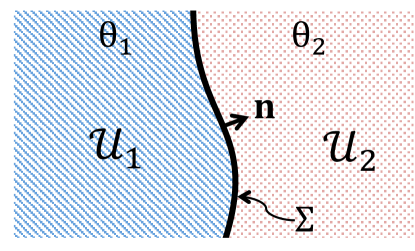
Figure 1: Region over which the electromagnetic field theory is defined.

$$\nabla\cdot\mathbf{E} = \tilde{\theta}\delta\left(F_{\Sigma}(\mathbf{x})\right)\mathbf{B}\cdot\mathbf{\hat{n}}+4\pi\rho,$$ (9)

$$\nabla\times\mathbf{B}-\frac{\partial\mathbf{E}}{\partial t} = \tilde{\theta}\delta\left(F_{\Sigma}(\mathbf{x})\right)\mathbf{E}\times\mathbf{\hat{n}}+4\pi\mathbf{J},$$ (10)

which reproduce the Eqs. (3) in this setting. The homogeneous equations are included in the Bianchi identity. Here $\mathbf{\hat{n}}$ is the unit normal to $\Sigma$ defined in Eq. (8), shown in Fig. 1 and $\tilde{\theta}=\alpha\left(\theta_{1}-\theta_{2}\right)/\pi$, which enforces the invariance of the classical action under the shifts of $\theta$ by any constant, $\theta\rightarrow\theta+C$. As we see from Eqs. (9-10) the behavior of $\theta$-ED in the bulk regions $\mathcal{U}_{1}$ and $\mathcal{U}_{2}$ is the same as in standard electrodynamics.

Assuming that the time derivatives of the fields are finite in the vicinity of the surface $\Sigma$, the field equations (9) and (10) imply that the normal component of $\mathbf{E}$, and the tangential components of $\mathbf{B}$, acquire discontinuities additional to those produced by superficial free charges and currents, while the normal component of $\mathbf{B}$, and the tangential components of $\mathbf{E}$, are continuous at the boundary. For vanishing external sources on $\Sigma$ the boundary conditions read:

$$\Delta\mathbf{E}_{n}\big{|}_{\Sigma} = \tilde{\theta}\mathbf{B}_{n}\big{|}_{\Sigma},\quad\Delta\mathbf{B}_{\parallel}\big{|}_{\Sigma}=-\tilde{\theta}\mathbf{E}_{\parallel}\big{|}_{\Sigma},$$ (11)

$$\Delta\mathbf{B}_{n}\big{|}_{\Sigma} = 0,\quad\Delta\mathbf{E}_{\parallel}\big{|}_{\Sigma}=0.$$ (12)

The notation $\Delta\mathbf{V}_{i}\big{|}_{\Sigma}$ refers to the discontinuity of the $i$-th component of the vector $\mathbf{V}$ across the interface $\Sigma$, while $\mathbf{V}_{j}\big{|}_{\Sigma}$ indicates the continuous value of the $j$-th component evaluated at $\Sigma$. The continuity conditions, (12), imply that the right hand sides of equations (11) are well defined and they represent surface charge and current densities, respectively. An immediate consequence of the boundary conditions (11) and (12) is that the presence of a magnetic field crossing the surface $\Sigma$ is sufficient to generate an electric surface charge density there, even in the absence of free electric charges.

3 The Green’s function method in a $\theta$-vacuum

In this section we review the Green’s function (GF) method to solve a class of static boundary-value problems in $\theta$-ED in terms of the electromagnetic potential $A^{\mu}$. Certainly one could solve for the electric and magnetic fields from the modified Maxwell equations together with the boundary conditions (11-12), however, just as in ordinary electrodynamics, there might be occasions where information about the sources is unknown and rather we are provided with information of the 4-potential at some given boundaries. In these cases, the GF method provides the general solution to such boundary-value problem (Dirichlet or Neumann) for arbitrary sources. Nevertheless, in the following we restrict ourselves to contributions of free sources only outside the $\theta$-boundary with no additional boundary conditions (BCs) besides those required at $\Sigma$. Also we consider the simplest media having $\theta_{1}\neq\theta_{2}$, but with $\varepsilon=1$ and $\mu=1$, which we call the $\theta$-vacuum.

In this case, the inhomogeneous Maxwell’s equations can be written as

$$\partial_{\mu}F^{\mu\nu}=\tilde{\theta}\delta\left(F_{\Sigma}(\mathbf{x})\right)n_{\mu}\tilde{F}^{\mu\nu}+4\pi j^{\nu},$$ (13)

Current conservation can be verified directly by taking the divergence on both sides of Eq. (13) and realizing that

$$\partial_{\nu}\left(\tilde{\theta}\delta\left(F_{\Sigma}(\mathbf{x})\right)n_{\mu}\tilde{F}^{\mu\nu}\right)=\tilde{\theta}\delta^{\prime}\left(F_{\Sigma}(\mathbf{x})\right)n_{\nu}n_{\mu}\tilde{F}^{\mu\nu}+\tilde{\theta}\delta\left(F_{\Sigma}(\mathbf{x})\right)n_{\mu}\partial_{\nu}\tilde{F}^{\mu\nu}$$ (14)

is zero by symmetry properties together with the Bianchi identity. Since the homogeneous Maxwell equations are not modified, the electrostatic and magnetostatic fields can be written in terms of the $4$-potential $A^{\mu}=\left(\phi,\mathbf{A}\right)$ according to $\mathbf{E}=-\nabla\phi$ and $\mathbf{B}=\nabla\times\mathbf{A}$ as usual. In the Coulomb gauge $\nabla\cdot\mathbf{A}=0$, the $4$-potential satisfies the equation of motion

$$\left[-\eta_{\phantom{\mu}\nu}^{\mu}\nabla^{2}-\tilde{\theta}\delta\left(F_{\Sigma}(\mathbf{x})\right)n_{\rho}\epsilon_{\;\;\;\;\ \nu}^{\rho\mu\alpha}\partial_{\alpha}\right]A^{\nu}=4\pi j^{\mu},$$ (15)

together with the boundary conditions

$$\Delta A^{\mu}\big{|}_{\Sigma}=0,\qquad\Delta\left(\partial_{z}A^{\mu}\right)\big{|}_{\Sigma}=-\tilde{\theta}\epsilon_{\;\;\;\;\ \nu}^{3\mu\alpha}\left(\partial_{\alpha}A^{\nu}\right)\big{|}_{\Sigma}.$$ (16)

One can further check that these boundary conditions for the $4$-potential correspond to those written in Eqs. (11-12).

To obtain a general solution for the potentials $\phi$ and $\mathbf{A}$ in the presence of arbitrary external sources $j^{\mu}(\mathbf{x})$, we introduce the GF $G_{\phantom{\nu}\sigma}^{\nu}\left(\mathbf{x},\mathbf{x}^{\prime}\right)$ solving Eq. (15) for a point-like source,

$$\left[-\eta_{\phantom{\mu}\nu}^{\mu}\nabla^{2}-\tilde{\theta}\delta\left(F_{\Sigma}(\mathbf{x})\right)n_{\rho}\epsilon_{\phantom{\rho}\phantom{\mu}\phantom{\alpha}\nu}^{\rho\mu\alpha}\partial_{\alpha}\right]G_{\phantom{\nu}\sigma}^{\nu}\left(\mathbf{x},\mathbf{x}^{\prime}\right)=4\pi\eta_{\;\sigma}^{\mu}\delta^{3}\left(\mathbf{x}-\mathbf{x}^{\prime}\right),$$ (17)

together with the boundary conditions (16), in such a way that the general solution for the $4$-potential in the Coulomb gauge is

$$A^{\mu}\left(\mathbf{x}\right)=\int d^{3}\mathbf{x}^{\prime}\;G_{\phantom{\mu}\nu}^{\mu}\left(\mathbf{x},\mathbf{x}^{\prime}\right)j^{\nu}\left(\mathbf{x}^{\prime}\right).$$ (18)

According to Eqs. (17) the diagonal entries of the GF matrix are related with the electric and magnetic fields arising from the charge and current density sources, respectively, although they acquire a $\theta$-dependence. However, the non-diagonal terms encode the magnetoelectric effect, i.e. the charge (current) density contributing to the magnetic (electric) field.

As we will show in the following, a further simplification in $\theta$-ED arises when the system satisfies the following two coordinate conditions:(i) the coordinate system can be chosen so that the interface $\Sigma$ is defined by setting constant only one of them and (ii) the Laplacian is separable in such coordinates in such a way that a complete orthonormal set of eigenfunctions can be defined in the subspace orthogonal to the coordinate defining the interface. Three cases show up immediately: (i) a plane interface at fixed $z$, (ii) a spherical interface at constant $r$ and (iii) a cylindrical interface at constant $\rho$. In all this cases the characteristic function $\theta\left(\mathbf{x}\right)\;$defined in Eq. (7)  can be written in terms of the Heaviside function $H$ of one coordinate in terms of $H(z-a),\;H(r-a)$ and $H(\rho-a)$, with the associated unit vectors $\mathbf{\hat{n}}_{\xi}\;$given by  $\mathbf{\hat{k}}$ , $\mathbf{\hat{r}\;}$and $\mathbf{\hat{\rho}}$, respectively, in each of the adapted coordinate systems. Then Eq. (17) reduces to

$$\left[-\eta_{\phantom{\mu}\nu}^{\mu}\nabla^{2}-\tilde{\theta}\delta\left(\xi-\xi_{0}\right)\epsilon_{\phantom{\xi}\phantom{\mu}\phantom{\alpha}\nu}^{\xi\mu\alpha}\partial_{\alpha}\right]G_{\phantom{\nu}\sigma}^{\nu}\left(\mathbf{x},\mathbf{x}^{\prime}\right)=4\pi\eta_{\phantom{\mu}\sigma}^{\mu}\delta^{3}\left(\mathbf{x}-\mathbf{x}^{\prime}\right),$$ (19)

where $\xi$ denotes the coordinate defining the interface at $\xi=\xi_{0}$ and the coupling of the $\theta$-term is given by a one dimensional delta function with support only in the coordinate that defines the interface. Also, the unit vector $\mathbf{\hat{n}}_{\xi}$ will have a component only in the direction $\xi$.

Let us consider the coordinates partitioned according to $\xi$ plus two additional ones which we denote by $\sigma$ and $\tau$. Also assume that the Laplacian can be separated in the form

$$\nabla^{2}=L_{1}(\xi)+f(\xi)L_{2}(\sigma,\tau)$$ (20)

where the operator $L_{2}(\sigma,\tau)\;$has eigenfunctions $\Psi_{M}(\sigma,\tau)\;$which form a complete orthonormal set in the subspace of the coordinates $\sigma,\tau$ (which we denote collectively by $\Pi$)

$$L_{2}(\sigma,\tau)\Psi_{M}(\sigma,\tau)=\lambda_{M}\Psi_{M}(\sigma,\tau),$$ (21)

where $M$ denote a set of discrete or continuous labels. The basic properties of  $\Psi_{M}(\sigma,\tau)$ are

$$\int d\mu(\sigma,\tau)\;\Psi_{M}^{\ast}(\sigma,\tau)\Psi_{M^{\prime}}(\sigma,\tau)=\delta_{M,M^{\prime}},\;\; \;\;\sum_{M}\Psi_{M}(\sigma,\tau)\Psi_{M}^{\ast}(\sigma^{\prime},\tau^{\prime})=\delta^{2}(\Pi-\Pi^{\prime}),\;$$

$$\int d\mu(\sigma,\tau)\delta^{2}(\Pi-\Pi^{\prime})=1$$ , (22)

where $d\mu$ denotes the integration measure in each subspace and $d^{3}\mathbf{x}=d\mu(\sigma,\tau)\;d\mu(\xi)$. Also we have

$$\;\delta^{3}\left(\mathbf{x}-\mathbf{x}^{\prime}\right)=\delta^{2}(\Pi-\Pi^{\prime})\delta(\xi-\xi^{\prime}),\;\;\;\int d\mu(\xi)\delta(\xi-\xi^{\prime})=1.$$

Next we introduce the reduced Green’s function$\;\;\left(g_{\;\sigma}^{\nu}\right)_{M,M^{\prime}}\left(\xi,\xi^{\prime}\right)\;$in the following way

$$G_{\phantom{\nu}\sigma}^{\nu}\left(\mathbf{x},\mathbf{x}^{\prime}\right)=4\pi\sum_{M,M^{\prime}}\Psi_{M}(\sigma,\tau)\Psi_{M^{\prime}}^{\ast}(\sigma^{\prime},\tau^{\prime})\left(g_{\phantom{\nu}\sigma}^{\nu}\right)_{M,M^{\prime}}\left(\xi,\xi^{\prime}\right)$$ (23)

When substituting Eq. (20) in Eq. (19) we obtain

$$\sum_{M,M^{\prime}}\Psi_{M}(\sigma,\tau)\Psi_{M^{\prime}}^{\ast}(\sigma^{\prime},\tau^{\prime})\left[-\eta_{\phantom{\mu}\nu}^{\mu}L_{1}(\xi)\right]\left(g_{\phantom{\nu}\sigma}^{\nu}\right)_{M,M^{\prime}}\left(\xi,\xi^{\prime}\right)$$ (24)

$$+\sum_{M,M^{\prime}}\Psi_{M}(\sigma,\tau)\Psi_{M^{\prime}}^{\ast}(\sigma^{\prime},\tau^{\prime})\left[-\eta_{\phantom{\mu}\nu}^{\mu}f(\xi)\lambda_{M}\right]\left(g_{\phantom{\nu}\sigma}^{\nu}\right)_{M,M^{\prime}}\left(\xi,\xi^{\prime}\right)$$

$$+\sum_{M,M^{\prime}}O_{\phantom{\mu}\nu}^{\mu}(\sigma,\tau)\Psi_{M}(\sigma,\tau)\Psi_{M^{\prime}}^{\ast}(\sigma^{\prime},\tau^{\prime})\left[-\tilde{\theta}\delta\left(\xi-\xi_{0}\right)\right]\left(g_{\phantom{\nu}\sigma}^{\nu}\right)_{M,M^{\prime}}\left(\xi,\xi^{\prime}\right)$$

$$= \eta_{\phantom{\mu}\sigma}^{\mu}\sum_{N,N^{\prime}}\Psi_{N}(\sigma,\tau)\Psi_{N^{\prime}}^{\ast}(\sigma^{\prime},\tau^{\prime}))\delta_{N,N^{\prime}}\delta(\xi-\xi^{\prime}),$$

since the operator

$$\epsilon_{\phantom{\xi}\phantom{\mu}\phantom{\alpha}\nu}^{\xi\mu\alpha}\partial_{\alpha}\equiv O_{\phantom{\mu}\nu}^{\mu}(\sigma,\tau)$$ (25)

contains only derivatives with respect to $\sigma,\tau$ so that it acts upon the functions $\Psi_{M}(\sigma,\tau)$. Multiplication to the right by $\Psi_{T}(\sigma^{\prime},\tau^{\prime})$ and integration over $d\mu(\sigma^{\prime},\tau^{\prime})$, followed by multiplication to the left by $\Psi_{P}^{\ast}(\sigma,\tau)$ and integration over $d\mu(\sigma,\tau)$ yields

$$\left[\left(L_{1}(\xi)+\lambda_{P}f(\xi)\right)\right]\left(g_{\phantom{\mu}\sigma}^{\mu}\right)_{P,T}\left(\xi,\xi^{\prime}\right) +\tilde{\theta}\delta\left(\xi-\xi_{0}\right)\sum_{M}\left[O_{\phantom{\mu}\nu}^{\mu}\right]_{PM}\left(g_{\phantom{\nu}\sigma}^{\nu}\right)_{M,T}\left(\xi,\xi^{\prime}\right)$$ (26)

$$=-\eta_{\phantom{\mu}\sigma}^{\mu}\delta_{P,T}\delta(\xi-\xi^{\prime}),$$

where we have introduced the following matrix element

$$\left[O_{\phantom{\mu}\nu}^{\mu}\right]_{PM}\equiv\int d\mu(\sigma,\tau)\Psi_{P}^{\ast}(\sigma,\tau)O_{\phantom{\mu}\nu}^{\mu}(\sigma,\tau)\Psi_{M}(\sigma,\tau)$$ (27)

which is independent of $\xi$ and $\xi^{\prime}$.

In this way we transform the calculation of the reduced GF into a one dimensional problem with a delta interaction. The above equation (26) can be directly integrated with the knowledge of an additional reduced GF $\left(\mathfrak{g}_{\phantom{\mu}\sigma}^{\mu}\right)_{P,T}\left(\xi,\xi^{\prime}\right)$, corresponding to the $\tilde{\theta}=0$ limit, which satisfies

$$\left[\left(L_{1}(\xi)+\lambda_{P}f(\xi)\right)\right]\left(\mathfrak{g}_{\phantom{\mu}\sigma}^{\mu}\right)_{P,T}\left(\xi,\xi^{\prime}\right)=-\eta_{\phantom{\mu}\sigma}^{\mu}\delta_{P,T}\delta(\xi-\xi^{\prime}),$$ (28)

plus boundary conditions.

The introduction of $\left(\mathfrak{g}_{\phantom{\mu}\sigma}^{\mu}\right)_{P,T}\left(\xi,\xi^{\prime}\right)$ derives from the existence of a full Green’s function

$$\mathfrak{G}_{\phantom{\nu}\sigma}^{\nu}\left(\mathbf{x},\mathbf{x}^{\prime}\right)=\sum_{M,M^{\prime}}\Psi_{M}(\sigma,\tau)\Psi_{M^{\prime}}^{\ast}(\sigma^{\prime},\tau^{\prime})\left(\mathfrak{g}_{\phantom{\nu}\sigma}^{\nu}\right)_{M,M^{\prime}}\left(\xi,\xi^{\prime}\right),$$ (29)

which must respect the coordinate conditions of the problem in a setting where the $\theta$-medium is absent. We refer to them as the free GF’s, emphasizing that they correspond to the $\tilde{\theta}=0$ case. These GF’s can be taken directly from the vast literature in standard electrodynamics and are the basis for finding the response of an identical system now in the presence of a $\theta$-medium, the interface of which defines the corresponding coordinate conditions. As an illustration take the case of a planar $\theta$-medium that can be embedded in two different ways: (i) either in vacuum, just by choosing the free GF $\mathfrak{G}_{\phantom{\nu}\sigma}^{\nu}\left(\mathbf{x},\mathbf{x}^{\prime}\right)$ with standard BCs at infinity, or (ii) between a pair of conducting plates of infinite extension which are parallel to the interface just by requiring $\mathfrak{G}_{\phantom{\nu}\sigma}^{\nu}\left(\mathbf{x},\mathbf{x}^{\prime}\right)$ to satisfy the appropriate BCs at the plates, which can be found in Ref. 29, for example. This approach was used in Ref. 30 when calculating the Casimir effect between parallel metallic plates in the presence of a planar $\theta$-medium and will be reviewed in section 5.

In terms of the free reduced GF $\left(\mathfrak{g}_{\phantom{\mu}\sigma}^{\mu}\right)_{P,T}\left(\xi,\xi^{\prime}\right)$ we obtain

$$\left(g_{\phantom{\mu}\sigma}^{\mu}\right)_{P,T}\left(\xi,\xi^{\prime}\right)=\left(\mathfrak{g}_{\phantom{\mu}\sigma}^{\mu}\right)_{P,T}\left(\xi,\xi^{\prime}\right)+\frac{\tilde{\theta}}{4\pi}\sum_{M,N}\left(\mathfrak{g}_{\phantom{\mu}\rho}^{\mu}\right)_{P,N}\left(\xi,\xi_{0}\right)\left[O_{\phantom{\rho}\nu}^{\rho}\right]_{NM}\left(g_{\phantom{\nu}\sigma}^{\nu}\right)_{M,T}\left(\xi_{0},\xi^{\prime}\right).$$ (30)

This result can be explicitly verified by applying the operator $\left[\left(L_{1}(\xi)+\lambda_{P}f(\xi)\right)\right]$ to Eq. (30) and using Eq. (28).

It is convenient to think of $\left(g_{\phantom{\mu}\sigma}^{\mu}\right)_{P,T},\;\left(\mathfrak{g}_{\phantom{\mu}\sigma}^{\mu}\right)_{P,T}$ and $\left[O_{\phantom{\rho}\nu}^{\rho}\right]_{NM}$ as generalized matrix elements of the operators $g,\;\mathfrak{g}$ and $O$, respectively. This allows us to rewrite Eq. (30) in the compact form

$$g\left(\xi,\xi^{\prime}\right)=\mathfrak{g}\left(\xi,\xi^{\prime}\right)+\frac{\tilde{\theta}}{4\pi}\mathfrak{g}\left(\xi,\xi_{0}\right)Og\left(\xi_{0},\xi^{\prime}\right).$$ (31)

This set of equations constitute a coupled system of algebraic equations which can be disentangled according to the following steps. First we set $\xi=\xi_{0}$ in Eq. (31)

$$g\left(\xi_{0},\xi^{\prime}\right)=\mathfrak{g}\left(\xi_{0},\xi^{\prime}\right)+\frac{\tilde{\theta}}{4\pi}\mathfrak{g}\left(\xi_{0},\xi_{0}\right)Og\left(\xi_{0},\xi^{\prime}\right)$$ (32)

and solve for $g\left(\xi_{0},\xi^{\prime}\right)$ as

$$g\left(\xi_{0},\xi^{\prime}\right)=\frac{1}{\left(1-\frac{\tilde{\theta}}{4\pi}\mathfrak{g}\left(\xi_{0},\xi_{0}\right)O\right)}\mathfrak{g}\left(\xi_{0},\xi^{\prime}\right).$$ (33)

Then we substitute the above result in Eq. (31) obtaining

$$g\left(\xi,\xi^{\prime}\right)=\mathfrak{g}\left(\xi,\xi^{\prime}\right)+\frac{\tilde{\theta}}{4\pi}\mathfrak{g}\left(\xi,\xi_{0}\right)O\frac{1}{\left(1-\frac{\tilde{\theta}}{4\pi}\mathfrak{g}\left(\xi_{0},\xi_{0}\right)O\right)}\mathfrak{g}\left(\xi_{0},\xi^{\prime}\right),$$ (34)

which expresses the reduced GF $\left(g_{\phantom{\mu}\sigma}^{\mu}\right)_{P,T}$ in terms of the free GF $\left(\mathfrak{g}_{\phantom{\mu}\sigma}^{\mu}\right)_{P,T}$. The full GF is reconstructed then from the Eq. (23). In the specific cases considered in Refs. 31, 32, 33 the solutions of Eqs. (33) and (34) are explicitly constructed in a step by step fashion to be illustrated in the next section.

4 The case of a planar interface

The simplest example of the construction previously discussed is when the interface $\Sigma$ is the plane $z=a$. Here the MEP $\theta(\mathbf{x})$ is

$$\theta(z)=\theta_{1}H(a-z)+\theta_{2}H(z-a),$$ (35)

where $H(z)$ is the Heaviside function. Then $\nabla\theta=(\theta_{2}-\theta_{1})\delta(z-a)\hat{\mathbf{e}}_{z}$, and $\hat{\mathbf{e}}_{z}$ is the unit vector in the direction $z$. In this way, the dynamical modifications in Eqs. (3) arise only at the boundary $z=a$, which is the only place where the effective sources (5) are nonzero. That is to say, the $\theta$-vacuum has conducting properties at the boundary $\Sigma$, even though its bulk behaves as ordinary vacuum. The general eigenfunctions in Eq. (21) take the form

$$\Psi_{\mathbf{p_{\parallel}}}(x,y)=\frac{1}{\left(2\pi\right)}e^{i\mathbf{p}_{\parallel}\cdot\mathbf{x}_{\parallel}}\;,\;$$ (36)

where the index $M$ is now the momentum $\mathbf{p}_{\parallel}=(p_{x},p_{y})$ parallel to the plane $\Sigma$ and $\mathbf{x}_{\parallel}=(x,y)$. This adds up to realize the Eq. (23) by introducing the reduced GF $\left(g_{\phantom{\mu}\nu}^{\mu}\right)_{\mathbf{p,p}^{\prime}}\left(z,z^{\prime}\right)$ as

$$G_{\phantom{\mu}\nu}^{\mu}\left(\mathbf{x},\mathbf{x}^{\prime}\right)=4\pi\int d^{2}\mathbf{p}_{\parallel}\mathbf{\;}d^{2}\mathbf{p}_{\parallel}^{\prime}\frac{1}{\left(2\pi\right)^{2}}e^{i\mathbf{p}_{\parallel}\cdot\left(\mathbf{x}-\mathbf{x}^{\prime}\right)_{\parallel}}\left(g_{\phantom{\mu}\nu}^{\mu}\right)_{\mathbf{p,p}^{\prime}}\left(z,z^{\prime}\right)$$ (37)

In this case the operator in Eq. (25) is $O_{\phantom{\mu}\ \nu}^{\mu}=\epsilon_{\phantom{z}\phantom{\mu}\phantom{\alpha}\nu}^{z\mu\alpha}\partial_{\alpha}$ and its matrix elements of Eq. (27) simplify to

$$\left[O_{\phantom{\mu}\nu}^{\mu}\right]_{\mathbf{p,p}^{\prime}}=\epsilon_{\phantom{3}\phantom{\mu}\phantom{\alpha}\nu}^{3\mu\alpha}ip_{\alpha}\delta^{2}(\mathbf{p}_{\parallel}\mathbf{-p}_{\parallel}^{\prime}),$$ (38)

where $p^{\alpha}=(0,p_{x},p_{y},0)=(0,\mathbf{p}_{\parallel})$. Since $\left[O_{\phantom{\mu}\nu}^{\mu}\right]_{\mathbf{p,p}^{\prime}}$ is diagonal in momentum space, Eq. (26) indicates that we can also take $\left(g_{\phantom{\mu}\nu}^{\mu}\right)_{\mathbf{p,p}^{\prime}}\left(z,z^{\prime}\right)$ to be diagonal, so that we write

$$\left(g_{\phantom{\mu}\nu}^{\mu}\right)_{\mathbf{p,p}^{\prime}}\left(z,z^{\prime}\right)=\delta^{2}(\mathbf{p}_{\parallel}\mathbf{-p}_{\parallel}^{\prime})g_{\phantom{\mu}\nu}^{\mu}\left(z,z^{\prime},\mathbf{p}_{\parallel}\right).$$ (39)

In this way, the final representation for the GF of Eq. (37) turns out to be given in terms of the Fourier transform in the directions $x,y$ parallel to the plane $\Sigma$ [29]

$$G_{\phantom{\mu}\nu}^{\mu}\left(\mathbf{x},\mathbf{x}^{\prime}\right)=4\pi\int\frac{d^{2}\mathbf{p_{\parallel}}}{\left(2\pi\right)^{2}}e^{i\mathbf{p}_{\parallel}\cdot\left(\mathbf{x}-\mathbf{x}^{\prime}\right)_{\parallel}}g_{\phantom{\mu}\nu}^{\mu}\left(z,z^{\prime},\mathbf{p}_{\parallel}\right),$$ (40)

as expected.

Due to the antisymmetry of the Levi-Civita symbol, the partial derivative appearing in the second term of the GF Eq. (17) does not introduce derivatives with respect to $z$, but only in the transverse directions. This allows us to write the full reduced GF equation as

$$\left[\partial^{2}\eta_{\phantom{\mu}\nu}^{\mu}+i\tilde{\theta}\delta\left(z-a\right)\epsilon_{\phantom{3}\phantom{\mu}\phantom{\alpha}\nu}^{3\mu\alpha}p_{\alpha}\right]g_{\phantom{\nu}\sigma}^{\nu}\left(z,z^{\prime},\mathbf{p},\right)=\eta_{\phantom{\mu}\sigma}^{\mu}\delta\left(z-z^{\prime}\right),$$ (41)

where $\partial^{2}=\mathbf{p}^{2}-\partial_{z}^{2}$, $p^{\alpha}p_{\alpha}=-\mathbf{p_{\parallel}}^{2}$ and we denote $|\mathbf{p_{\parallel}}|=p$.

The solution of Eq. (41) is obtained with the introduction of a reduced free GF having the form $\mathfrak{G}_{\phantom{\mu}\nu}^{\mu}\left(z,z^{\prime}\right)=\mathfrak{g}\left(z,z^{\prime}\right)\eta_{\phantom{\mu}\nu}^{\mu}$, associated with the operator $\partial^{2}$ previously defined, that solves

$$\partial^{2}\mathfrak{G}_{\phantom{\mu}\nu}^{\mu}\left(z,z^{\prime}\right)=\eta_{\phantom{\mu}\nu}^{\mu}\delta\left(z-z^{\prime}\right),$$ (42)

plus BC’s. In the case of standard BC’s at infinity, the choice is [29]

$$\mathfrak{g}(z,z^{\prime})=\frac{1}{2p}e^{-p|z-z^{\prime}|}.$$ (43)

Note that Eq. (42) demands the derivative of $\mathfrak{g}$ to be discontinuous at $z=z^{\prime}$, i.e., $\partial_{z}\mathfrak{g}\left(z,z^{\prime}\right)\big{|}_{z=z^{\prime-}}^{z=z^{\prime+}}=-1$, together with the continuity of $\mathfrak{g}$ at $z=z^{\prime}$.

Now we observe that Eq. (41) can be directly integrated by using the free GF in Eq. (42) together with the properties of the Dirac delta-function, thus reducing the problem to a set of coupled algebraic equations,

$$g_{\phantom{\mu}\sigma}^{\mu}\left(z,z^{\prime}\right)=\eta_{\phantom{\mu}\sigma}^{\mu}\mathfrak{g}\left(z,z^{\prime}\right)-i\tilde{\theta}\epsilon_{\phantom{3}\phantom{\mu}\phantom{\alpha}\nu}^{3\mu\alpha}p_{\alpha}\mathfrak{g}\left(z,a\right)g_{\phantom{\nu}\sigma}^{\nu}\left(a,z^{\prime}\right).$$ (44)

Note that the continuity of $\mathfrak{g}$ at $z=z^{\prime}$ implies the continuity of $g_{\phantom{\mu}\sigma}^{\mu}$, but the discontinuity of $\partial_{z}\mathfrak{g}$ at the same point yields

$$\partial_{z}g_{\phantom{\mu}\sigma}^{\mu}\left(z,z^{\prime}\right)\big{|}_{z=a^{-}}^{z=a^{+}}=-i\tilde{\theta}\epsilon_{\phantom{3}\phantom{\mu}\phantom{\alpha}\nu}^{3\mu\alpha}p_{\alpha}\partial_{z}\mathfrak{g}\left(z,a\right)\big{|}_{z=a^{-}}^{z=a^{+}}g_{\phantom{\nu}\sigma}^{\nu}\left(a,z^{\prime}\right)=i\tilde{\theta}\epsilon_{\phantom{3}\phantom{\mu}\phantom{\alpha}\nu}^{3\mu\alpha}p_{\alpha}g_{\phantom{\nu}\sigma}^{\nu}\left(a,z^{\prime}\right),$$ (45)

from which the boundary conditions for the 4-potential in Eq. (16) are recovered. In this way the solution in Eq. (44) guarantees that the boundary conditions at the $\theta$-interface are satisfied.

In this case the formal solution for Eq. (34) for $g_{\phantom{\mu}\sigma}^{\mu}\left(z,z^{\prime}\right)$ can be explicitly obtained in successive steps. To this end we split Eq. (44) into $\mu=0$ and $\mu=j=1,2,3$ components;

$$g_{\phantom{0}\sigma}^{0}\left(z,z^{\prime}\right) = \eta_{\phantom{0}\sigma}^{0}\mathfrak{g}\left(z,z^{\prime}\right)-i\tilde{\theta}\epsilon_{\phantom{3}\phantom{0}\phantom{i}j}^{30i}p_{i}\mathfrak{g}\left(z,a\right)g_{\phantom{j}\sigma}^{j}\left(a,z^{\prime}\right),$$ (46)

$$g_{\phantom{j}\sigma}^{j}\left(z,z^{\prime}\right) = \eta_{\phantom{j}\sigma}^{j}\mathfrak{g}\left(z,z^{\prime}\right)-i\tilde{\theta}\epsilon_{\phantom{3}\phantom{j}\phantom{i}0}^{3ji}p_{i}\mathfrak{g}\left(z,a\right)g_{\phantom{0}\sigma}^{0}\left(a,z^{\prime}\right).$$ (47)

Now we set $z=a$ in Eq. (47) and then substitute into Eq. (46) yielding

$$g_{\phantom{0}\sigma}^{0}\left(z,z^{\prime}\right)=\eta_{\phantom{0}\sigma}^{0}\mathfrak{g}\left(z,z^{\prime}\right)-i\tilde{\theta}\epsilon_{\phantom{3}\phantom{0}\phantom{i}j}^{30i}p_{i}\eta_{\phantom{j}\sigma}^{j}\mathfrak{g}\left(z,a\right)\mathfrak{g}\left(a,z^{\prime}\right)-\tilde{\theta}^{2}p^{2}\mathfrak{g}\left(z,a\right)\mathfrak{g}\left(a,a\right)g_{\phantom{0}\sigma}^{0}\left(a,z^{\prime}\right),$$ (48)

where we use the result $\epsilon_{\phantom{3}\phantom{0}\phantom{i}j}^{30i}\epsilon_{\phantom{3}\phantom{j}\phantom{k}0}^{3jk}\,p_{k}p_{i}=p^{2}$. Solving for $g_{\phantom{0}\sigma}^{0}\left(a,z^{\prime}\right)$ by setting $z=a$ in Eq. (48) and inserting the result back in Eq. (48), we obtain

$$g_{\phantom{0}\sigma}^{0}\left(z,z^{\prime}\right)=\eta_{\phantom{0}\sigma}^{0}\left[\mathfrak{g}\left(z,z^{\prime}\right)+\tilde{\theta}p^{2}\mathfrak{g}\left(a,a\right)A\left(z,z^{\prime}\right)\right]+i\epsilon_{\phantom{3}\phantom{0}\phantom{i}\sigma}^{30i}p_{i}A\left(z,z^{\prime}\right),$$ (49)

where

$$A\left(z,z^{\prime}\right)=-\tilde{\theta}\frac{\mathfrak{g}\left(z,a\right)\mathfrak{g}\left(a,z^{\prime}\right)}{1+p^{2}\tilde{\theta}^{2}\mathfrak{g}^{2}\left(a,a\right)}.$$ (50)

The remaining components can be obtained by substituting $g_{\phantom{0}\sigma}^{0}\left(a,z^{\prime}\right)$ in Eq. (47). The result is

$$g_{\phantom{j}\sigma}^{j}\left(z,z^{\prime}\right)=\eta_{\phantom{j}\sigma}^{j}\mathfrak{g}\left(z,z^{\prime}\right)+i\epsilon_{\phantom{3}\phantom{j}\phantom{k}0}^{3jk}p_{k}\left[\eta_{\phantom{0}\sigma}^{0}-i\tilde{\theta}\epsilon_{\phantom{3}\phantom{0}\phantom{i}\sigma}^{30i}p_{i}\mathfrak{g}\left(a,a\right)\right]A\left(z,z^{\prime}\right).$$ (51)

Equations (49) and (51) allow us to write the general solution as

$$g_{\phantom{\mu}\nu}^{\mu}\left(z,z^{\prime}\right)=\eta_{\phantom{\mu}\nu}^{\mu}\mathfrak{g}\left(z,z^{\prime}\right)+A\left(z,z^{\prime}\right)\left\{\tilde{\theta}\mathfrak{g}\left(a,a\right)\left[p^{\mu}p_{\nu}+\left(\eta_{\phantom{\mu}\nu}^{\mu}+n^{\mu}n_{\nu}\right)p^{2}\right]+i\epsilon_{\phantom{\mu}\nu}^{\mu\phantom{\nu}\alpha 3}p_{\alpha}\right\},$$ (52)

where $n_{\mu}=\left(0,0,0,1\right)$ is the normal to $\Sigma$

The reciprocity between the position of the unit charge and the position at which the GF is evaluated $G_{\mu\nu}(\mathbf{x},\mathbf{x}^{\prime})=G_{\nu\mu}(\mathbf{x}^{\prime},\mathbf{x})$ is one of its most remarkable properties of the GF. From Eq. (40) this condition demands

$$g_{\mu\nu}(z,z^{\prime},\mathbf{p})=g_{\nu\mu}(z^{\prime},z,-\mathbf{p}),$$ (53)

which we verify directly from Eq. (52). The symmetry $g_{\mu\nu}\left(z,z^{\prime}\right)=g_{\nu\mu}^{\ast}\left(z,z^{\prime}\right)=g_{\mu\nu}^{\dagger}\left(z,z^{\prime}\right)$ is also manifest.

The various components of the static GF matrix in coordinate representation are obtained by computing the Fourier transform defined in Eq. (40), with the reduced GF given by Eq. (43). The details are presented in Ref. 31. The final results are

$$G_{\phantom{0}0}^{0}\left(\mathbf{x},\mathbf{x}^{\prime}\right) = \frac{1}{|\mathbf{x}-\mathbf{x}^{\prime}|}-\frac{\tilde{\theta}^{2}}{4+\tilde{\theta}^{2}}\frac{1}{\sqrt{R^{2}+Z^{2}}},$$ (54)

$$G_{\phantom{0}i}^{0}\left(\mathbf{x},\mathbf{x}^{\prime}\right) = -\frac{2\tilde{\theta}}{4+\tilde{\theta}^{2}}\frac{\epsilon_{0ij3}R^{j}}{R^{2}}\left(1-\frac{Z}{\sqrt{R^{2}+Z^{2}}}\right),$$ (55)

$$G_{\phantom{i}j}^{i}\left(\mathbf{x},\mathbf{x}^{\prime}\right) = \eta_{\phantom{i}j}^{i}G_{\;0}^{0}\left(\mathbf{x},\mathbf{x}^{\prime}\right)-\frac{i}{2}\frac{\tilde{\theta}^{2}}{4+\tilde{\theta}^{2}}\partial^{i}K_{j}\left(\mathbf{x},\mathbf{x}^{\prime}\right),$$ (56)

where $Z=|z-a|+|z^{\prime}-a|$, $R^{j}=\left(\mathbf{x-x}^{\prime}\right)_{\parallel}^{j}=\left(x-x^{\prime},y-y^{\prime}\right)$, $R=|\left(\mathbf{x-x}^{\prime}\right)_{\parallel}|\;$and

$$K^{j}\left(\mathbf{x},\mathbf{x}^{\prime}\right)=2i\frac{\sqrt{R^{2}+Z^{2}}-Z}{R^{2}}R^{j}.$$ (57)

Finally, we observe that Eqs. (54-56) contain all the required elements of the GF matrix, according to the choices of $z$ and $z^{\prime}$ in the function $Z$.

Similar results for the cases of spherical and cylindrical interfaces incorporating also piecewise continuous ponderable media have been reported in Refs. 32, 33.

5 The Casimir effect

The Casimir effect (CE) [34] is one of the most remarkable consequences of the nonzero vacuum energy predicted by quantum field theory which has been confirmed by experiments [35]. In general, the CE can be defined as the stress (force per unit area) on bounding surfaces when a quantum field is confined in a finite volume of space. The boundaries can be material media, interfaces between two phases of vacuum, or topologies of space. For a review see, for example, Refs. 36, 37.

The experimental accessibility to micrometer-size physics together with the recent discovery of three dimensional TIs [38] provides an additional arena where the CE can be studied. In the scattering approach to the Casimir effect, i.e. using the Fresnel coefficients for the reflection matrices at the interfaces of the TIs, the Casimir force between TIs was computed in Ref. 39. The authors found the most notable feature that, due to the magnetoelectric effect, which now has a topological origin, the strength and sign of the Casimir stress between two planar TIs can be tuned.

When the surface of the TI is included in the description, $\theta$-ED is a fair description of both the bulk and the surface only when a time reversal symmetry breaking perturbation is induced on the surface to gap the surface states, thereby converting it into a full insulator. In this situation, which we consider here, the MEP $\theta$ can be shown to be quantized in odd integer values of $\pi$: $\theta=(2n+1)\pi$, where $n\in\mathbb{Z}$ is determined by the nature of the time reversal symmetry breaking perturbation, which could be controlled experimentally by covering the TI with a thin magnetic layer [39]. For a review of the effective $\theta$-ED describing the electromagnetic response of TI’s see Refs. 10, 14 for example.

The Casimir system we consider is formed by two perfectly reflecting planar surfaces (labeled $P_{1}$ and $P_{2}$) separated by a distance $L$, with a non-trivial TI placed between them, but perfectly joined to the plate $P_{2}$, as shown in Fig. 2. The surface $\Sigma$ of the TI, located at $z=a$, is assumed to be covered by a thin magnetic layer which breaks time reversal symmetry there. We calculate the Casimir stress restricting ourselves only to the contribution of the MEP which now has a topological origin, i.e. we set $\varepsilon=\mu=1$. We follow an approach similar to that in Ref. 40 which starts from the calculation of the appropriate GF, to subsequently compute the renormalized vacuum stress-energy tensor in the region between the plates yielding finally the Casimir stress that the plates exert on the surface $\Sigma$ of the TI. We also consider the limit where the plate $P_{2}$ is sent to infinity ($L\rightarrow\infty$) to obtain the Casimir stress between a conducting plate and a non-trivial semi-infinite TI.

The BCs for the perfectly reflecting metallic plates $P_{1}$ and $P_{2}$ are the standard ones $n_{\mu}\tilde{F}^{\mu\nu}|_{P_{1,2}}=0$, where $n_{\mu}=(0,0,0,1)$. The effects of the MEP are incorporated by choosing

$$\theta(z)=\theta H(z-a)H(L-z),\quad\tilde{\theta}=-\alpha\theta/\pi.$$ (58)

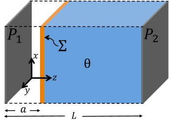
Figure 2: Schematic of the Casimir effect in $\theta$-ED.

Assuming the absence of free sources on $\Sigma$, the required equation for the GF matrix is given by Eq. (17), together with the BCs arising from Eq. (16). The calculation proceeds along the same lines discussed in section 4 for the static case, but keeping the time dependence now. Making explicit the coordinate choice in the transverse $x$ and $y$ directions we can write

$$G_{\phantom{\mu}\nu}^{\mu}\left(x,x^{\prime}\right)=4\pi\int\frac{d^{2}\mathbf{p_{\parallel}}}{\left(2\pi\right)^{2}}e^{i\mathbf{p_{\parallel}}\cdot\mathbf{x_{\parallel}}}\int\frac{d\omega}{2\pi}e^{-i\omega(t-t^{\prime})}g_{\phantom{\mu}\nu}^{\mu}\left(z,z^{\prime}\right),$$ (59)

where we have omitted the dependence of the reduced GF $g_{\phantom{\mu}\nu}^{\mu}$ on $\omega$ and $\mathbf{p_{\parallel}}$. In the Lorenz gauge the equation for the reduced GF $g_{\phantom{\nu}\sigma}^{\nu}(z,z^{\prime})$ is

$$\left[\eta_{\phantom{\mu}\nu}^{\mu}\partial^{2}+i\tilde{\theta}\delta\left(z-a\right)\epsilon_{\phantom{3\mu\alpha}\nu}^{3\mu\alpha}p_{\alpha}\right]g_{\phantom{\nu}\sigma}^{\nu}\left(z,z^{\prime}\right)=\eta_{\phantom{\mu}\sigma}^{\mu}\delta\left(z-z^{\prime}\right),$$ (60)

where now $\partial^{2}=\mathbf{p_{\parallel}}^{2}-\omega^{2}-\partial_{z}^{2}$ and $p^{\alpha}=\left(\omega,\mathbf{p_{\parallel}},0\right)$. The boundary term (at $z=L$), missing in Eq. (60), identically vanishes in the distributional sense, due to the BCs on the plate $P_{2}$. In this way, Eq. (60) implies that the only topologically magnetoelectric effect present in our Casimir system is the one produced at $\Sigma$.

Here the free GF we use to integrate Eq. (60) is the reduced GF for two parallel conducting surfaces placed at $z=0$ and $z=L$, which is the solution of $\partial^{2}\mathfrak{g}\left(z,z^{\prime}\right)=\delta\left(z-z^{\prime}\right)$ satisfying the BCs $\mathfrak{g}\left(0,z^{\prime}\right)=\mathfrak{g}\left(L,z^{\prime}\right)=0$, namely [29]

$$\mathfrak{g}_{c}\left(z,z^{\prime}\right)=\frac{\sin\left[pz_{<}\right]\sin\left[p\left(L-z_{>}\right)\right]}{p\sin\left[pL\right]},$$ (61)

where $z_{>}$ ($z_{<}$) is the greater (lesser) of $z$ and $z^{\prime}$, and $p=\sqrt{\omega^{2}-\textbf{p}^{2}}$. Now the problem is reduced to a set of coupled algebraic equations,

$$g^{\mu}_{\phantom{\mu}\sigma}\left(z,z^{\prime}\right)=\eta^{\mu}_{\phantom{\mu}\sigma}\mathfrak{g}_{c}\left(z,z^{\prime}\right)-i\tilde{\theta}\epsilon^{3\mu\alpha}_{\phantom{3\mu\alpha}\nu}p_{\alpha}\mathfrak{g}_{c}\left(z,a\right)g^{\nu}_{\phantom{\nu}\sigma}\left(a,z^{\prime}\right).$$ (62)

We write the general solution to Eq. (62) as the sum of two terms

$$g^{\mu}_{\phantom{\mu}\nu}\left(z,z^{\prime}\right)=\eta^{\mu}_{\phantom{\mu}\nu}\mathfrak{g}_{c}\left(z,z^{\prime}\right)+{g}^{\mu}_{C\nu}\left(z,z^{\prime}\right).$$ (63)

The first term provides the propagation in the absence of the TI between the parallel plates. The second, to be called the reduced $\theta$-GF, which can be shown to be

$$g^{\mu}_{C\nu}\left(z,z^{\prime}\right)=\tilde{\theta}\mathfrak{g}_{c}\left(a,a\right)\left[p^{\mu}p_{\nu}-\left(\eta^{\mu}_{\phantom{\mu}\nu}+n^{\mu}n_{\nu}\right)p^{2}\right]A_{c}\left(z,z^{\prime}\right)+i\,\epsilon^{\mu\phantom{\nu}\alpha 3}_{\phantom{\mu}\nu}p_{\alpha}A_{c}\left(z,z^{\prime}\right),$$

(64)

encodes the magnetoelectric effect due to the topological MEP $\theta$. Here

$$A_{c}\left(z,z^{\prime}\right)=-\tilde{\theta}\frac{\mathfrak{g}_{c}\left(z,a\right)\mathfrak{g}_{c}\left(a,z^{\prime}\right)}{1-p^{2}\tilde{\theta}^{2}\mathfrak{g}_{c}^{2}\left(a,a\right)},$$ (65)

has the same form as the previous Eq. (50) with $\mathfrak{g}\left(z,z^{\prime}\right)\rightarrow\mathfrak{g}_{c}\left(z,z^{\prime}\right)$. In the static limit ($\omega=0$), our result in Eq. (64) reduces to the one reported in Ref. 31. As the Eq. (63) suggests, the full GF matrix $G^{\mu}_{\phantom{\mu}\nu}\left(x,x^{\prime}\right)$ can also be written as the sum of two terms, $G^{\mu}_{\phantom{\mu}\nu}\left(x,x^{\prime}\right)=\eta^{\mu}_{\phantom{\mu}\nu}\mathcal{G}\left(x,x^{\prime}\right)+G^{\mu}_{C\nu}\left(x,x^{\prime}\right)$, each one arising from the respective term in the Eq. (63). We call $G^{\mu}_{C\nu}\left(x,x^{\prime}\right)$ the $\theta$-GF.

Since the MEP modifies the behavior of the fields only at the interface, we expect that stress energy tensor (SET) in the bulk retains its original Mawxwell’s form. In fact, in Ref. 32 we explicitly computed the SET and verified that

$$T^{\mu\nu}=\frac{1}{4\pi}\left(-F^{\mu\lambda}F^{\nu}_{\phantom{\nu}\lambda}+\frac{1}{4}\eta^{\mu\nu}F_{\alpha\beta}F^{\alpha\beta}\right).$$ (66)

Clearly this tensor is traceless and its divergence is

$$\partial_{\mu}T^{\mu\nu}=-F^{\nu}_{\phantom{\nu}\lambda}j^{\lambda}-(\tilde{\theta}/4\pi)\delta\left(\Sigma\right)n_{\mu}F^{\nu}_{\phantom{\nu}\lambda}\tilde{F}^{\mu\lambda}.$$ (67)

As expected, $T^{\mu\nu}$ it is not conserved at $\Sigma$ because the MEP induces effective charge and current densities there.

Now we address the calculation of the vacuum expectation value of the SET, to which we will refer simply as the vacuum stress (VS). The local approach to compute the VS was initiated by Brown and Maclay who calculated the renormalized stress tensor by means of GF techniques [40, 41]. Using the standard point splitting procedure and taking the vacuum expectation value of the SET in (66) we find

$$\left<T^{\mu\nu}\right>=\frac{i}{4\pi}\lim_{x\rightarrow x^{\prime}}\Big{[}-\partial^{\mu}\partial^{\prime\nu}G^{\lambda}_{\phantom{\lambda}\lambda}+\partial^{\mu}\partial_{\lambda}^{\prime}G^{\lambda\nu}+\partial^{\lambda}\partial^{\prime\nu}G^{\mu}_{\phantom{\mu}\lambda}$$

$$-\,\partial^{\prime\lambda}\partial_{\lambda}G^{\mu\nu}+\frac{1}{2}\eta^{\mu\nu}\left(\partial^{\alpha}\partial_{\alpha}^{\prime}G^{\lambda}_{\phantom{\lambda}\lambda}-\partial^{\alpha}\partial_{\beta}^{\prime}G^{\beta}_{\phantom{\beta}\alpha}\right)\Big{]},$$ (68)

where we have omitted the dependence of $G^{\mu\nu}$ on $x$ and $x^{\prime}$. This result can be further simplified as follows. Since the GF is written as the sum of two terms, the VS can also be written in the same way, i.e.,

$$\left<T^{\mu\nu}\right>=\left<t^{\mu\nu}\right>+\left<T_{C}^{\mu\nu}\right>.$$ (69)

The first term,

$$\left<t^{\mu\nu}\right>=\frac{1}{4\pi i}\lim_{x\rightarrow x^{\prime}}\left(2\partial^{\mu}\partial^{\prime\nu}-\frac{1}{2}\eta^{\mu\nu}\partial^{\lambda}\partial_{\lambda}^{\prime}\right)\mathcal{G}\left(x,x^{\prime}\right),$$ (70)

is the VS in the absence of the TI. In obtaining Eq. (70) we use that the GF is diagonal when the TI is absent, i.e. it is equal to $\eta^{\mu}_{\phantom{\mu}\nu}\mathcal{G}\left(x,x^{\prime}\right)$. The second term $\left<T_{C}^{\mu\nu}\right>$, to which we will refer as the $\theta$ vacuum stress ($\theta$-VS), can be simplified since the $\theta$-GF satisfies the Lorenz gauge condition $\partial_{\mu}G_{C}^{\mu\nu}=0$.

With the previous results the $\theta$-VS can be written as

$$\left<T_{C}^{\mu\nu}\right>=\frac{1}{4\pi i}\lim_{x\rightarrow x^{\prime}}\left[\partial^{\mu}\partial^{\prime\nu}G_{C}+\partial^{\prime\lambda}\partial_{\lambda}\left(G_{C}^{\mu\nu}-\frac{1}{2}\eta^{\mu\nu}G_{C}\right)\right],$$ (71)

where $G_{C}=G^{\mu}_{C\mu}$ is the trace of the $\theta$-GF. This result exhibits the vanishing of the trace at quantum level, i.e., $\eta_{\mu\nu}\left<T_{C}^{\mu\nu}\right>=0$.

Next we consider the problem of calculating the renormalized VS $\left<T^{\mu\nu}\right>_{\mathrm{ren}}$. We proceed along the lines of Refs. 40, 42. From Eq. (71), together with the symmetry of the problem we find that the $\theta$-VS can be written as

$$\left<T_{C}^{\mu\nu}\right>=i\tilde{\theta}\int\frac{d^{2}\mathbf{p_{\parallel}}}{(2\pi)^{2}}\int\frac{d\omega}{2\pi}\left(p^{\mu}p^{\nu}+n^{\mu}n^{\nu}p^{2}\right)\mathfrak{g}_{c}\left(a,a\right)\lim_{z\rightarrow z^{\prime}}\left(p^{2}+\partial^{\prime}_{z}\partial_{z}\right)A_{c}\left(z,z^{\prime}\right).$$

(72)

In deriving this result we used the Fourier representation of the GF in Eq. (40) together with the solution for the reduced $\theta$-GF given by Eq. (64). From Eq. (72) we calculate the renormalized $\theta$-VS, which is given by $\left<T_{C}^{\mu\nu}\right>_{\mathrm{ren}}=\left<T_{C}^{\mu\nu}\right>-\left<T_{C}^{\mu\nu}\right>_{\mathrm{vac}}$, where the first (second) term is the $\theta$-VS in the presence (absence) of the plates [42]. When the plates are absent, the reduced GF we have to use to compute the $\theta$-VS in the region $[0,L]$ is that of the free-vacuum $\mathfrak{g}_{0}(z,z^{\prime})=(i/2p){\rm exp}(ip|z-z^{\prime}|)$, from which we find that $\lim_{z\rightarrow z^{\prime}}\partial_{z}\partial_{z}^{\prime}A_{0}\left(z,z^{\prime}\right)=-p^{2}\lim_{z\rightarrow z^{\prime}}A_{0}\left(z,z^{\prime}\right)$, thus implying that the integrand in Eq. (72) vanishes. The function $A_{0}$ is given by Eq. (50) using the free-vacuum reduced GF $\mathfrak{g}_{0}(z,z^{\prime})$. Therefore we conclude that $\left<T^{\mu\nu}_{C}\right>_{vac}=0$.

Next we compute $\left<T^{\mu\nu}_{C}\right>_{\mathrm{ren}}=\left<T^{\mu\nu}_{C}\right>$ starting from Eq. (72). From the symmetry of the problem, the components of the stress along the plates, $\left<T^{11}_{C}\right>$ and $\left<T^{22}_{C}\right>$, are equal. In addition, from the mathematical structure of Eq. (72) we find the relation $\left<T^{00}_{C}\right>=-\left<T^{11}_{C}\right>$. These results, together with the traceless nature of the SET, allow us to write the renormalized $\theta$-VS in the form

$$\left<T^{\mu\nu}_{C}\right>_{\mathrm{ren}}=\left(\eta^{\mu\nu}+4n^{\mu}n^{\nu}\right)\tau(\theta,z)\;,$$ (73)

where

$$\tau(\theta,z) = i\tilde{\theta}\int\frac{d^{2}\mathbf{p_{\parallel}}}{(2\pi)^{2}}\int\frac{d\omega}{2\pi}\omega^{2}\mathfrak{g}_{c}\left(a,a\right)\lim_{z\rightarrow z^{\prime}}\left(p^{2}+\partial^{\prime}_{z}\partial_{z}\right)A_{c}\left(z,z^{\prime}\right).$$ (74)

Our $\theta$-VS exhibits the same tensor structure as the result obtained by Brown and Maclay [40], but now a $z$-dependent VS arises since the SET is not conserved at $\Sigma$. Using Eq. (61) we compute the limit of the integrand in Eq. (74) obtaining

$$\lim_{z\rightarrow z^{\prime}}\left(p^{2}+\partial_{z}\partial_{z}^{\prime}\right)P\left(z,z^{\prime}\right)=-\frac{\tilde{\theta}}{1-\tilde{\theta}^{2}p^{2}\mathfrak{g}_{c}^{2}\left(a,a\right)}\times$$

$$\left\{\frac{\sin^{2}\left[p\left(L-a\right)\right]}{\sin^{2}\left[pL\right]}H\left(a-z\right)+\frac{\sin^{2}\left[pa\right]}{\sin^{2}\left[pL\right]}H\left(z-a\right)\right\}.$$ (75)

To evaluate the integral in Eq. (24) we first write the momentum element as $d^{2}\mathbf{p_{\parallel}}=|\mathbf{p_{\parallel}}|d|\mathbf{p_{\parallel}}|d\vartheta$ and integrate $\vartheta$. Next, we perform a Wick rotation such that $\omega\rightarrow i\zeta$, then replace $\zeta$ and $|\mathbf{p_{\parallel}}|$ by plane polar coordinates $\zeta=\xi\cos\varphi$, $|\mathbf{p_{\parallel}}|=\xi\sin\varphi$ and finally integrate $\varphi$. The renormalized $\theta$-VS in Eq. (73) then becomes

$$\left<T^{\mu\nu}_{C}\right>_{\mathrm{ren}}=-\frac{\pi^{2}}{720L^{4}}\left(\eta^{\mu\nu}+4n^{\mu}n^{\nu}\right)\left[u({\theta},\chi)H\left(a-z\right)+u({\theta},1-\chi)H\left(z-a\right)\right],$$

(76)

where

$$u({\theta},\chi)=\frac{120}{\pi^{4}}\int_{0}^{\infty}\frac{{\tilde{\theta}}^{2}\xi^{3}\mbox{\small sh}\left[\xi\chi\right]\mbox{\small sh}^{3}\left[\xi\left(1-\chi\right)\right]\mbox{\small sh}^{-3}\left[\xi\right]}{1+{\tilde{\theta}}^{2}\mbox{\small sh}^{2}\left[\xi\chi\right]\mbox{\small sh}^{2}\left[\xi\left(1-\chi\right)\right]\mbox{\small sh}^{-2}\left[\xi\right]}d\xi,$$ (77)

with $\mbox{\small sh}(x)=\sinh(x)$ and $\chi=a/L$ with $0<\chi<1$. Physically, we interpret the function $u({\theta},\chi)$ as the ratio between the renormalized $\theta$-energy density in the vacuum region $[0,a)$ and that of the renormalized energy density in the absence of the TI. The function $u({\theta},1-\chi)$ has an analogous interpretation for the bulk region of the TI $(a,L]$. This shows that the energy density is constant in the bulk regions, however a simple discontinuity arises at $\Sigma$, i.e., $\partial_{z}\left<T^{00}_{C}\right>_{\mathrm{ren}}\propto\delta(\Sigma)$. The Casimir energy ${\cal E}={\cal E}_{L}+{\cal E}_{\theta}$ is defined as the energy per unit area stored in the electromagnetic field between the plates. To obtain it we must integrate the contribution from the $\theta$-energy density

$$\mathcal{E}_{\theta}=\int_{0}^{L}dz\left<T^{00}_{C}\right>_{\mathrm{ren}}={\mathcal{E}}_{L}\left[\chi u({\theta},\chi)+(1-\chi)u({\theta},1-\chi)\right].$$ (78)

The first term corresponds to the energy stored in the electromagnetic field between $P_{1}$ and $\Sigma$, while the second term is the energy stored in the bulk of the TI. The ratio $\mathcal{E}_{\theta}/{\mathcal{E}}_{L}$ as a function of $\chi$ for different values of $\theta$ (appropriate for TIs [39]) is plotted in Fig. 3 [30]. Let us recall that $\mathcal{E}_{L}=-\pi^{2}/(720L^{3})$ is the Casimir energy in the absence of the TI.

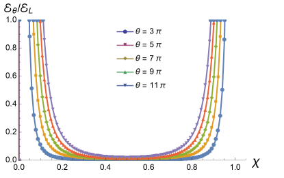
Figure 3: The ratio $\mathcal{E}_{\theta}/\mathcal{E}_{L}$ as a function of the dimensionless distance $\chi=a/L$, for different values of $\theta$.

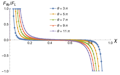
Figure 4: The Casimir stress on the $\theta$-piston in units of $F_{L}$ as a function of $\chi=a/L$, for different values of $\theta$.

The setup known in the literature as the Casimir piston consists of a rectangular box of length $L$ divided by a movable mirror (piston) at a distance $a$ from one of the plates [43]. The net result is that the Casimir energy in each region generates a force on the piston pulling it towards the nearest end of the box. Here we have considered a similar setup, which we call the $\theta$-piston, in which the piston is the TI. The Casimir stress acting upon $\Sigma$ can be obtained as $F_{\theta p}=-d\mathcal{E}_{\theta}/da$. The result is

$$\frac{F_{\theta p}}{F_{L}}=-\frac{1}{3}\frac{d}{d\chi}\left[\chi u(\theta,\chi)+(1-\chi)u(\theta,1-\chi)\right],$$ (79)

where $F_{L}--\pi^{2}/(240L^{4})$ is the Casimir stress between the two perfectly reflecting plates in the absence of the TI. Figure 4 [30] shows the Casimir stress on $\Sigma$ in units of $F_{L}$ as a function of $\chi$ for different values of $\theta$. We observe that this force pulls the boundary $\Sigma$ towards the closer of the two fixed walls $P_{1}$ or $P_{2}$, similarly to the conclusion in Ref. 43.

Now let us consider the limit where the plate $P_{2}$ is sent to infinity, i.e., $L\rightarrow\infty$. This configuration corresponds to a perfectly conducting plate $P_{1}$ in vacuum, and a semi-infinite TI located at a distance $a$. Here the plate and the TI exert a force upon each other. The Casimir energy in Eq. (78) in the limit $L\rightarrow\infty$ takes the form $\mathcal{E}_{\theta}^{L\rightarrow\infty}={\mathcal{E}}_{a}R(\theta)$, with ${\mathcal{E}}_{a}=-\pi^{2}/720a^{3}$, and the function

$$R(\theta)=\frac{120}{\pi^{4}}\int_{0}^{\infty}\xi^{3}\frac{\tilde{\theta}^{2}}{1+\tilde{\theta}^{2}e^{-2\xi}\sinh^{2}\xi}e^{-3\xi}\sinh\xi d\xi,$$ (80)

is $a$-independent and bounded by its $\theta\rightarrow\pm\infty$ limit, i.e.,

$$R(\theta)\leq\frac{120}{\pi^{4}}\int_{0}^{\infty}\xi^{3}\frac{e^{-\xi}}{\sinh\xi}d\xi=1.$$ (81)

Thus, for this case, the energy stored in the electromagnetic field is bounded by the Casimir energy between two parallel conducting plates at a distance $a$, i.e., $\mathcal{E}_{\theta}^{L\rightarrow\infty}\leq{\mathcal{E}}_{a}$. Physically this implies that in the $\theta\rightarrow\infty$ limit the surface of the TI mimics a conducting plate, which is analogous to Schwinger’s prescription for describing a conducting plate as the $\varepsilon\rightarrow\infty$ limit of material media [29]. These results, which stem from our Eqs. (64) and (50), agree with those obtained in the global energy approach which uses the reflection matrices containing the Fresnel coefficients as in Ref. 39, when the appropriate limits to describe an ideal conductor at $P_{1}$ and a purely topological surface at $\Sigma$ are taken into account. Taking the derivative with respect to $a$ we find that the plate and the TI exert a force (in units of $F_{a}=-\pi^{2}/240a^{4}$) of attraction upon each other given by $f_{\theta}=F^{L\rightarrow\infty}_{\theta}/F_{a}=R(\theta)$. Numerical results for $f_{\theta}$ for different values of $\theta$ are presented in Table 5.

Normalized force $f_{\theta}=F^{L\rightarrow\infty}_{\theta}/F_{a}=R(\theta)$ for different values of $\theta$. $\theta$ $\pm 7\pi$ $\pm 15\pi$ $\pm 23\pi$ $\pm 31\pi$ $\pm 39\pi$ $f_{\theta}$ 0.0005 0.0025 0.0060 0.0109 0.0172

A general feature of our analysis is that the TI induces a $\theta$-dependence on the Casimir stress, which could be used to measure $\theta$. Since the Casimir stress has been measured for separation distances in the $0.5-3.0\,\mu$m range [35], these measurements require TIs of width lesser than $0.5\mu$m and an increase of the experimental precision of two to three orders of magnitude. In practice the ability to measure $f_{\theta}$ depends on the value of the topological MEP, which is quantized as $\theta=(2n+1)\pi,\,n\in\mathbb{Z}$. The particular values $\theta=\pm 7\pi,\pm 15\pi$ are appropriate for the TIs such as Bi_1-xSe_x [44], where we have $f_{\pm 7\pi}\approx 0.0005$ and $f_{\pm 15\pi}\approx 0.0025$, which are not yet feasible with the present experimental precision. This effect could also be explored in TIs described by a higher coupling $\theta$, such as Cr₂O₃. However, this material induces more general magnetoelectric couplings not considered in our model [39].

Although the reported $\theta$-effects of our Casimir systems cannot be observed in the laboratory yet, we have aimed to establish the Green’s function method as an alternative theoretical framework for dealing with the topological magnetoelectric effect of TIs and also as yet another application of the GF method we developed in Ref. 31, 32, 33.

References

• [1] J. C. Maxwell, A Dynamical Theory of the Electromagnetic Field, Phil. Trans. R. Soc. London 155, 459 (1865).
• [2] J. S. Schwinger, On Quantum-Electrodynamics and the Magnetic Moment of the Electron, Phys. Rev. 73, 416 (1948).
• [3] J. S. Schwinger, Quantum Electrodynamics I. A covariant Formulation, Phys. Rev. 74, 1439 (1948).
• [4] J. S. Schwinger, Quantum Electrodynamics II. Vacuum Polarization and Self Energy, Phys. Rev. 75, 651 (1949).
• [5] C. Nash and S. Sen, Topology and Geometry for Physicists (London: Academic Press Inc, 1983.)
• [6] K. Fujikawa and H. Suzuki, Path Integrals and Quantum Anomalies (Oxford: Clarendon Press, 2004).
• [7] M. Dine, TASI Lectures on the Strong CP Problem arXiv:0011376 [hep-ph],2000.
• [8] D. Birmingham, M. Blau, M. Radowski and G. Thompson, Topological field theory Phys. Rep. 209, 129 (1991).
• [9] M. Kuster, G. Raffelt and B. Beltrán (eds), Axions: Theory, Cosmology, and Experimental Searches (Lecture Notes in Physics vol 741) (Berlin: Springer-Verlag, 2008).
• [10] X. L. Qi , T. L. Hughes and S. C. Zhang, Topological field theory of time-reversal invariant insulators, Phys. Rev. B 78, 195424 (2008).
• [11] T. H. O’Dell, The Electrodynamics of Magneto-Electric Media (North-Holland, Amsterdam, 1970); L. D. Landau, E. M. Lifshitz and L. P. Pitaevskii, Electrodynamics of Continuous Media (Course of Theoretical Physics vol 8) (Oxford: Pergamon Press, 1984).
• [12] E. Plum, J. Zhou, J. Dong, V. A. Fedotov, T. Koschny, C. M. Soukoulis and N. I. Zheludev, Metamaterial with negative index due to chirality, Phys. Rev. B 79, 035407 (2009).
• [13] M. M. Vazifeh and M. Franz, Electromagnetic Response of Weyl Semimetals, Phys. Rev. Lett. 111, 027201 (2013).
• [14] X. L. Qi, Field-Theory Foundations of Topological Insulators, in Topological Insulators (Contemporary Concepts of Condensed Matter Science), eds.M. Franz and L. Molenkamp , Vol. 6 (Amsterdam: Elsevier, 2013).
• [15] N. P. Armitage, E. J. Mele and A. Vishwanath, Weyl and Dirac semimetals in three-dimensional solids, Rev. Mod. Phys. 90, 015001 (2018).
• [16] I. E. Dzyaloshinskii, On the Magneto-Electrical Effect in Antiferromagnets, JETP 37, 881 (1959).
• [17] D. N. Astrov, The Magneto-Electrical Effect in Antiferromagnets, JETP 38, 984 (1960).
• [18] M. Fiebig, Revival of the magnetoelectric effect, J. Phys. D: Appl. Phys. 38, R123 (2005).
• [19] V. Diziom, A. Shuvaev, A. Pimentov et al., Observation of the universal magnetoelectric effect in a 3D topological insulator, Nature Communications 8, 15297 (2017).
• [20] X. L. Qi, R. Li, J. Zang and S. C. Zhang, Inducing a magnetic monopole with topological surface States, Science 323, 1184 (2009).
• [21] C. Kim, E. Koh, and K. Lee, Janus and Multifaced Supersymmetric Theories, Journal of High Energy Physics, 0806, 040 (2008).
• [22] C. Kim, E. Koh, and K. Lee, Janus and multifaced supersymmetric theories. II, Phys. Rev. D 79, 126013 (2009).
• [23] F. Wilczek, Two applications of axion electrodynamics, Phys. Rev. Lett. 58, 1799 (1987).
• [24] L. Huerta and J. Zanelli, Optical properties of a $\theta$ vacuum, Phys. Rev. D 85, 085024 (2012).
• [25] Y. N. Obukhov and F. W. Hehl, Measuring a piecewise constant axion field in classical electrodynamics, Phys. Lett. A 341, 357 (2005).
• [26] A. Martín-Ruiz and L. F. Urrutia, Interaction of a hydrogenlike ion with a planar topological insulator, Phys. Rev. A 97, 022502 (2018).
• [27] A. Martín-Ruiz and E. Chan-López, Dynamics of a Rydberg hydrogen atom near a topologically insulating surface, Eur. Phys. Lett. 119, 53001 (2017)
• [28] J. D. Jackson, Classical Electrodynamics (Hoboken NJ: John Wiley & Sons, 1999).
• [29] J. Schwinger, L. DeRaad, K. Milton and W. Tsai, Classical Electrodynamics, Advanced Book Program, (Perseus Books 1998).
• [30] A. Martín-Ruiz, M. Cambiaso and L. F. Urrutia, A Green’s function approach to the Casimir effect on topological insulators with planar symmetry, Eur. Phys. Lett. 113, 60005 (2016).
• [31] A. Martín-Ruiz, M. Cambiaso and L. F. Urrutia, A Green’s function approach to Chern-Simons extended electrodynamics: An effective theory describing topological insulators, Phys. Rev. D 92, 125015 (2015).
• [32] A. Martín-Ruiz, M. Cambiaso and L. F. Urrutia, Electro- and magnetostatics of topological insulators as modeled by planar, spherical, and cylindrical $\theta$ boundaries: Green’s function approach Phys. Rev. D 93, 045022 (2016).
• [33] A. Martín-Ruiz, M. Cambiaso and L. F. Urrutia, Electromagnetic description of three-dimensional time-reversal invariant ponderable topological insulators, Phys. Rev. D 94, 085019 (2016).
• [34] H. B. G. Casimir, On the attraction between two perfectly conducting plates, Proc. K. Ned. Akad. Wet. 51, 793 (1948).
• [35] G. Bressi et al, Measurement of the Casimir Force between Parallel Metallic Surfaces, Phys. Rev. Lett. 88, 041804 (2002).
• [36] K. A. Milton, The Casimir effect: Physical Manifestation of Zero-Point Energy (World Scientific, Singapore, 2001).
• [37] M. Bordag, G. L. Klimchitskaya, U. Mohideen and V. M. Mostepanenko, Advances in Casimir effect (Oxford University Press, Great Britain, 2009).
• [38] L. Fu, C. L. Kane, and E. J. Mele, Topological Insulators in Three Dimensions, Phys. Rev. Lett. 98, 106803 (2007); D. Hsieh, D. Qian, L. Wray, Y. Xia, Y. S. Hor, R. J. Cava and M. Z. Hasan, A topological Dirac insulator in a quantum spin Hall phase, Nature 452, 970 (2008).
• [39] A. G. Grushin and A. Cortijo, Tunable Casimir Repulsion with Three-Dimensional Topological Insulators, Phys. Rev. Lett. 106, 020403 (2011); A. G. Grushin, P. Rodriguez-Lopez and A. Cortijo, Effect of finite temperature and uniaxial anisotropy on the Casimir effect with three-dimensional topological insulators, Phys. Rev. B 84, 045119 (2011).
• [40] L. S. Brown and G. J. Maclay, Vacuum Stress between Conducting Plates: An Image Solution, Phys. Rev. 184, 1272 (1969).
• [41] J. Schwinger, L. DeRaad and K. Milton, Casimir effect in dielectrics, Ann. Phys. (N.Y.) 115, 1 (1978).
• [42] D. Deutsch and P. Candelas, Boundary effects in quantum field theory, Phys. Rev. D 20, 3063 (1979).
• [43] R. M. Cavalcanti, Casimir force on a piston, Phys. Rev. D 69, 065015 (2004).
• [44] X. Zhou, et al, Photonic spin Hall effect in topological insulators, Phys. Rev. A 88, 053840 (2013).