Robustness of anomaly-related magnetoresistance in doped Weyl semimetals

Abstract

Weyl semimetal with Weyl fermions at Fermi energy is one of the topological materials, and is a condensed-matter realization of the relativistic fermions. However, there are several crucial differences such as the shift of Fermi energy, which can hinder the expected interesting physics. Chiral anomaly is a representative nontrivial phenomenon associated with Weyl fermions, which dictates the transfer of fermions between the Weyl fermions with opposite chirality; it is manifested as the negative magnetoresistance. Here we demonstrate that the magnetoresistance is robust against the deviation from the ideal Weyl Hamiltonian such as the shifted Fermi energy and nonlinear dispersions. We study a model with the energy dispersion containing two Weyl nodes, and find that the magnetoresistance persists even when the Fermi level is far away from the node, even above the saddle point that separates the two nodes. Surprisingly, the magnetoresistance remains even after the pair annihilation of the nodes.

I Introduction

Quantum anomaly, the violation of conservation laws by quantum effect, has a long history of study in the field of quantum field theory, deeply rooted in its foundation Fujikawa and Suzuki (2004). One such phenomenon is the chiral anomaly, which was initially discovered in the problem of photon self-energy Fujikawa and Suzuki (2004); Fukuda and Miyamoto (1949); Fukuda et al. (1949a, b); Steinberger (1949). Later, the violation of the chiral symmetry was also discovered in the electromagnetic response of Weyl Hamiltonian Vilenkin (1980); Nielsen and Ninomiya (1983), where the conservation of the chiral charge is violated in presence of both electric and magnetic field Nielsen and Ninomiya (1983). Interestingly, it was also pointed out that a similar phenomenon can be captured by a semiclassical transport theory, by taking into account the Berry phase effect Son and Spivak (2013). While these studies on the magneto-transport phenomena revealed the effect of quantum anomalies on transport phenomena, experimental investigation in high-energy physics remains unexplored due to the lack of experimentally accessible Weyl fermions.

Theoretical predictions of the Weyl fermions in ferromagnetic metals Fang et al. (2003) and also semimetals, i.e., Weyl semimetals, (WSMs) Herring (1937); Murakami (2007); Burkov and Balents (2011); Xu et al. (2011); Wan et al. (2011) opened the possible studies of chiral anomaly in solids. This theoretical possibility is indeed realized by the discovery of three-dimensional Dirac Liu et al. (2014); Neupane et al. (2014) and Weyl Lv et al. (2015); Xu et al. (2015) semimetals. These materials are considered to be an experimental platform for studying unique responses in Dirac and Weyl fermions to the electromagnetic field Oka and Aoki (2009); Potter et al. (2014); Moll et al. (2016); Taguchi et al. (2016); Ebihara et al. (2016); Chan et al. (2016); Ishizuka et al. (2016); Wu et al. (2016); Ishizuka et al. (2017); Chan et al. (2017); Ma et al. (2017); de Juan et al. (2017); Osterhoudt et al. ; Zhang et al. (2018a, b). Furthermore, the realization in solids allowed experimental generation of pseudo-electromagnetic fields by magnetic fluctuations Liu et al. (2013) and by lattice strains Guinea et al. (2009); Levy et al. (2010); Chernodub et al. (2014); Cortijo et al. (2015); Pikulin et al. (2016); Sumiyoshi and Fujimoto (2016); Grushin et al. (2016); Cortijo et al. (2016); Gorbar et al. (2017); Tchoumakov et al. (2017); Kariyado , providing greater freedom in experiments to study rich physics related to Weyl semimetals, such as the quantum anomaly.

In experiments, the chiral anomaly is often investigated by transport experiments where the anomaly is predicted to gives rise to negative longitudinal magnetoresistance (LMR) Nielsen and Ninomiya (1983); Fukushima et al. (2008); Son and Spivak (2013); Sekine et al. (2017); the LMR experiment is carried out in several Weyl and Dirac semimetals Liang et al. (2014); Huang et al. (2015); Xiong et al. (2015); Li et al. (2016a); Zhang et al. (2016); Hirschberger et al. (2016); Kuroda et al. (2017); Niemann et al. (2017); Zhang et al. (2017), showing negative magnetoresistance which is seemingly consistent with the theoretical predictions. The experimental confirmation of chiral anomaly, however, still remains a controversial issue. In part, this is a technical problem related to the distinction between different mechanisms for negative LMR, which was recently investigated experimentally Liu et al. (2018). A more fundamental problem, on the other hand, remains on the validity of the Weyl Hamiltonian. Unlike its counterpart in the high-energy theory, the realistic effective theory for the existing Weyl and Dirac semimetals turns out to be somewhat complicated than the Weyl Hamiltonian; the Weyl Hamiltonian only applies to a limited energy range often below the Fermi energy. For example, in Cd₃As₂, the Fermi level of the material is above the saddle point that separates the two nodes [Fig. 1(d)]. This situation in the materials cast doubt on how match of the physics of Weyl fermions survives in these materials. Nevertheless, a negative LMR similar to that in other WSM materials is recently observed in Cd₃As₂ Li et al. (2016b); Nishihaya et al. (2018); naively, this implies one of the two possibilities: the physics related to chiral anomaly is robust (appears in a rather general class of models with Weyl nodes) or the observed LMR is not related to the chiral anomaly. Despite the controversial situation, systematic theoretical investigation on such issues remains unexplored.

In this work, we study the general features of anomaly-related magnetoresistance. In particular, we study the anomaly-related LMR when the chemical potential is away from the Weyl nodes, considering both the semiclassical region under a weak magnetic field and quantum region in the presence of strong magnetic field where the Landau levels are well formed. In the semiclassical limit, we derive a general formula for the anomaly-related ${\cal O}(B^{2}E)$ response, which is related to the Berry curvature. The formula explicitly shows that the contribution to the anomaly-related LMR does not cancel out even when all nodes are enclosed in a Fermi surface, i.e., when the Fermi level is far away from the Weyl nodes. The formula also implies that no abrupt decrease of the anomaly-related current occurs at the Lifshitz point where the Fermi surfaces of the Weyl nodes merge. We demonstrate these results by applying the theory to a model with two Weyl nodes [Fig. 1(c) and 1(d)]. We discuss that the anomaly-related LMR robustly remains even when the Fermi level is far above the saddle point separating the two nodes [Fig. 1(d)], and no abrupt decrease occurs at the $\mu=m^{2}$, when the chemical potential reaches the saddle point of dispersion that connects the two Weyl nodes. This result indicates that the anomaly-related current of similar magnitude should be observed even when the Fermi level is above the saddle point, as long as the chemical potential is in the same order as the energy of the saddle point. On the other hand, the LMR under the strong-magnetic-field case is more dependent on the details of the model; a clear LMR appears only in the strong-field limit, if the lowest Landau level crosses the Fermi level. However, whether the chiral mode (lowest Landau level) crosses the Fermi level depends on the details of the Hamiltonian and the chemical potential. The behavior of the conductivity when the Fermi level is above the saddle point is shown in Fig. 1(a), where the black solid line is for the case in which the chiral mode exists at the Fermi level and the dashed line is for the case when the chiral mode is away from the Fermi level. In addition, we find that a remnant LMR exists even when the Weyl nodes vanish by the pair annihilation. We also reveal the critical behavior around this gap opening transition. The result indicates that the negative LMR in the semiclassical region robustly remains, especially in the weak-field limit, providing a strong evidence for the existence of Weyl nodes and/or in close vicinity of the Weyl semimetal (WSM) phase.

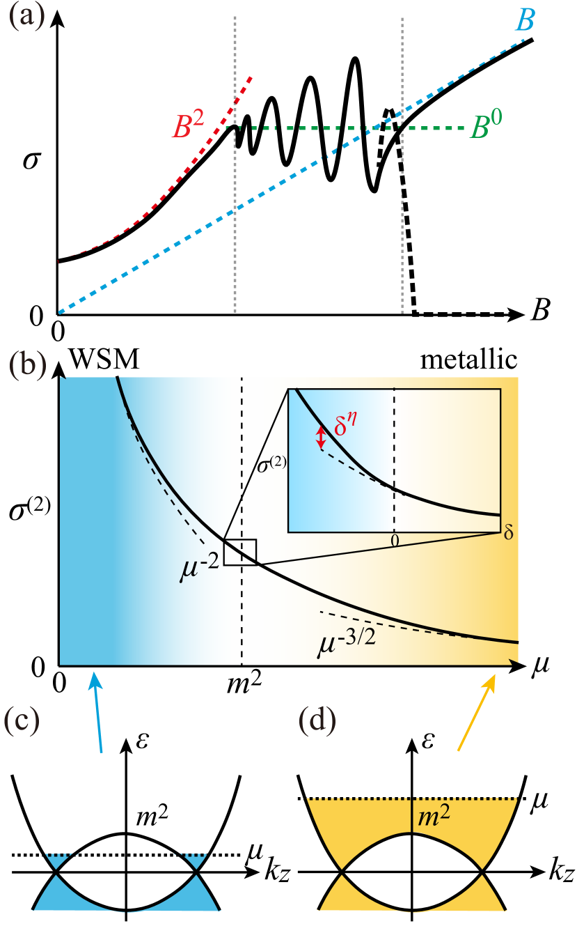
Figure 1: The conductivity of Weyl semimetals. (a) Field dependence of the longitudinal conductivity when the magnetic field is applied parallel to the electric field. The conductivity shows three regions: the semiclassical region under the weak field, quantum oscillation region in the intermediate field, and the high-field limit which either the lowest Landau level (solid line) or no Landau level (dashed line) crosses the Fermi level [See Fig. 4(b) and related arguments in the main text.]. The behavior of conductivity is for the case in which the chemical potential is much higher than the saddle point [the case shown in (d)]. (b) Schematic figure of the chemical potential ($\mu$) dependence of the ${\cal O}(B^{2})$ part of the conductivity in the semiclassical region when the electric and magnetic fields are parallel. The chemical potential dependence of the ${\cal O}(B^{2})$ conductivity changes from $\mu^{-2}$ in the $\mu\ll m^{2}$ to $\mu^{-3/2}$ in the $\mu\gg m^{2}$ limit. When the fields are along $a=x,y$, it shows non-analytic structure below the saddle point with $\eta=3/2$; such behavior vanishes for $a=z$ when $\bm{B}\parallel\bm{E}$. A schematic figure of the two Weyl nodes and the electron filling for $\mu\ll m^{2}$ and $\mu\gg m^{2}$ are shown in (c) and (d), respectively.

II Negative magnetoresistance in semiclassical transport theory

To investigate the behavior of anomaly-related phenomena when the Fermi level is away from the Weyl nodes, we first consider the case of the weak magnetic-field limit $\omega_{c}\tau\ll 1$, where $\omega_{c}$ is the cyclotron frequency of the electrons and $\tau$ is the relaxation time. We reformulate the semiclassical Boltzmann theory for magnetoresistance and explicitly show that, if the anomaly-related current exists, the sign of anomaly-related magnetoresistance is negative for arbitrary Hamiltonian. Moreover, the formula we introduce directly shows that the contribution from different nodes do not cancel out even when the Fermi level is away from the Weyl nodes and all nodes are enclosed in a Fermi surface.

We start from the semiclassical Boltzmann theory with Berry phase collection Sundaram and Niu (1999); Xiao et al. (2010). In the Boltzmann theory, the electron density $n_{\bm{k}\alpha}$ for band $\alpha$ and momentum $\bf k$ is calculated from the Boltzmann equation

$$\partial_{t}n_{\bm{k}\alpha}+\left(1+q\bm{B}\cdot\bm{b}_{\bm{k}\alpha}\right)^{-1}$$

$$\times\left(q\bm{E}+q\bm{v}_{\bm{k}\alpha}\times\bm{B}+q^{2}(\bm{E}\cdot\bm{B})\bm{b}_{\bm{k}\alpha}\right)\cdot\nabla_{\bm{k}}n_{\bm{k}\alpha}=-\frac{\delta n_{\bm{k}\alpha}}{\tau},$$ (1)

where $q$ is the charge of the particle and $\bm{E}\equiv(E_{x},E_{y},E_{z})$ [$\bm{B}\equiv(B_{x},B_{y},B_{z})$] is the electric (magnetic) field; $n_{\bm{k}\alpha}$, $\bm{v}_{\bm{k}\alpha}$, and $\bm{b}_{\bm{k}\alpha}$ are respectively the occupation, group velocity, and the Berry curvature. We here used the relaxation time approximation where $\tau$ is the relaxation time, $\delta n_{\bm{k}\alpha}\equiv n_{\bm{k}\alpha}-n_{\bm{k}\alpha}^{0}$ and $n_{\bm{k}\alpha}^{0}=f_{0}(\varepsilon_{\bm{k}\alpha})$ is the Fermi-Dirac distribution function with $\varepsilon_{\bm{k}\alpha}$ being the energy of the state.

To study the general features of the anomaly-related transport phenomena, we generalize the Berry phase formalism developed in Ref. Son and Spivak, 2013. Several forms of the generalizations of Ref. Son and Spivak, 2013 was attempted in several recent works for Weyl HamiltoniansKim et al. (2014); Lundgren et al. (2014); Sharma et al. (2016); McCormick et al. (2017); Gao et al. (2017); Sekine et al. (2017); Sharma et al. (2017); Wei et al. (2018). However, here, we reformulate the formula in a form which explicitly shows that the LMR from the anomaly-related current always gives a negative contribution to LMR. In the semiclassical Boltzmann theory, the electric current reads

$$\bm{J}=\sum_{\alpha}\int\frac{d\bm{k}}{(2\pi)^{3}}\left[\bm{v}_{\bm{k}\alpha}+q\bm{E}\times\bm{b}_{\bm{k}\alpha}+\frac{q}{c}(\bm{b}_{\bm{k}\alpha}\cdot\bm{v}_{\bm{k}\alpha})\bm{B}\right]n_{\bm{k}\alpha},$$ (2)

where $q$ is the charge of the particle and $\bm{E}\equiv(E_{x},E_{y},E_{z})$ [$\bm{B}\equiv(B_{x},B_{y},B_{z})$] is the electric (magnetic) field; $n_{\bm{k}\alpha}$, $\bm{v}_{\bm{k}\alpha}$, and $\bm{b}_{\bm{k}\alpha}$ are respectively the occupation, group velocity, and the Berry curvature of electrons with crystal momentum $\bm{k}$ and band index (including spin) $\alpha$. Note that the first term in the integrand of Eq. (2) corresponds to the conventional current, the second term to the intrinsic anomalous Hall effect (AHE), while the third term is the anomaly related contribution which is the main interest of the present paper. Assuming the steady state ($\partial_{t}n_{\bm{k}\alpha}=0$), and solving the Boltzmann equation in Eq. (1), we find

$$\delta n_{\bm{k}\alpha} =-\tau\left(1+q\bm{B}\cdot\bm{b}_{\bm{k}\alpha}\right)^{-1}\times$$

$$\left(q\bm{E}+q\bm{v}_{\bm{k}\alpha}\times\bm{B}+q^{2}(\bm{E}\cdot\bm{B})\bm{b}_{\bm{k}\alpha}\right)\bm{v}_{\bm{k}\alpha}\;(n_{\bm{k}\alpha}^{0})^{\prime},$$ (3)

where $(n_{\bm{k}\alpha}^{0})^{\prime}\equiv\partial_{\varepsilon}n^{0}(\varepsilon_{\bm{k}\alpha})$ is the derivative of the Fermi distribution function. We here expanded the solution up to second order in the electromagnetic fields, and linear order in the relaxation time.

Substituting this equation into Eq. (2), the anomaly-related response in the order of ${\cal O}(EB^{2})$ reads

$$\bm{J}_{\text{ano}}= \tau q^{4}\sum_{\alpha}\int\frac{dk^{3}}{(2\pi)^{3}}\bm{W}_{\bm{k}\alpha}[\bm{E}\cdot\bm{W}_{\bm{k}\alpha}]\delta(\varepsilon_{\bm{k}\alpha}-\mu),$$ (4)

where $\bm{W}_{\bm{k}\alpha}\equiv\bm{b}_{\bm{k}\alpha}\times(\bm{v}_{\bm{k}\alpha}\times\bm{B})$. Suppose we apply the electric field along a unit vector $\bm{e}_{E}$. Then, the current along $\bm{e}_{E}$ reads

$$(J_{\text{ano}}\cdot\bm{e}_{E})= \tau q^{4}E\sum_{\alpha}\int\frac{dk^{3}}{(2\pi)^{3}}(\bm{e}_{E}\cdot\bm{W}_{\bm{k}\alpha})^{2}\delta(\varepsilon_{\bm{k}\alpha}-\mu),$$ (5)

where $E=|\bm{E}|$. Therefore, the Berry phase contribution to LMR exists if the region of $\bm{k}$ with $\bm{W}_{\bm{k}\alpha}\neq 0$ has a finite measure on the Fermi surface. This essentially indicates that a nonzero negative LMR appears when $\bm{b}_{\bm{k}\alpha}\neq 0$, as there is no reason to be $W_{\bm{k}\alpha}=0$ on the entire Fermi surface unless $b_{\bm{k}\alpha}=0$. In WSMs, this also implies that the anomaly-related LMR appears even when all Weyl nodes are enclosed inside one Fermi surface; in this case, the total charge of Weyl nodes are zero, but the Berry curvature induced by the Weyl nodes (and $\bm{W}_{\bm{k}\alpha}$) are still nonzero, in general. Another interesting consequence of Eq. (5) is that the induced current along the electric field direction always gives a negative contribution to the resistivity, i.e., the anomaly-related LMR is always negative. These general features imply that the anomaly-related LMR in WSMs are also robust, regardless of the details of Hamiltonian. Moreover, the result indicates that the contribution from different Weyl nodes does not cancel out even when the Fermi level is away from the Weyl nodes and all nodes are enclosed in one Fermi surface.

We next consider the case in which $\bm{E}$ and $\bm{B}$ are perpendicular to each other. Applying $\bm{E}\cdot\bm{B}=0$ to Eq. (4), we find

$$( J_{\text{ano}}\cdot\bm{e}_{E})=$$

$$\tau q^{4}E\sum_{\alpha}\int\frac{dk^{3}}{(2\pi)^{3}}(\bm{e}_{E}\cdot\bm{v}_{\bm{k}\alpha})^{2}(\bm{B}\cdot\bm{b}_{\bm{k}\alpha})^{2}\delta(\varepsilon_{\bm{k}\alpha}-\mu).$$ (6)

Hence, similar to the case of LMR, negative magnetoresistance due to the Berry curvature also appears when $\bm{B}\perp\bm{E}$. Therefore, a negative magnetoresistance in the $\bm{E}\perp\bm{B}$ can appear even within the free electron approximation. In real materials, however, this contribution competes with the conventional magnetoresistance which gives a positive contribution Gao et al. (2017). Therefore, the sign of the magnetoresistance depends on the details of the band structure. We also note that this term remains finite also for the Weyl Hamiltonian in contrast to Ref. Son and Spivak, 2013, in which the anomaly-related current vanish when $\bm{E}\perp\bm{B}$. This is difference originates from the different approximation used for the electron distribution; we used the standard relaxation-time approximation while Ref. Son and Spivak, 2013 considered a limit where intra-node scattering is much faster than the inter-node ones. Further discussion on the sensitivity to the electron distribution is given in Appendix B.

In the last, we note that a similar argument on the amount of charge in each electron/hole pockets in the Brillouin zone shows that the rate of charge pumped between different pockets is determined only by the total charge of magnetic monopoles inside the pocket. This implies that the chiral charge pumping by the chiral anomaly is also robust. Details on this argument are given in Appendix A.

III Anomaly-related current in the weak magnetic field

III.1 Two-node model

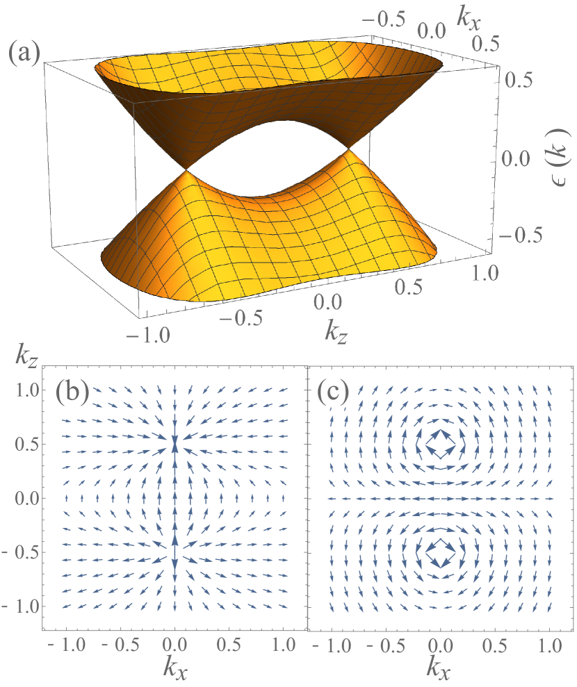
Figure 2: Band structure and Berry curvature distribution in the two-node model. (a) The band structure of the two-node Weyl Hamiltonian. (b) Berry curvature distribution of the two-node Weyl Hamiltonian in the $k_{y}=0$ plane, and (c) distribution of $\bm{W}_{+}(\bm{k})$ of the same Hamiltonian. The results are for $m=1/2$.

In this section, we apply the general argument presented in Sec. II to a model with two Weyl nodes and study how the anomaly-related response typically behaves with changing $\mu$. The Hamiltonian reads

$$H_{\rm DW}= \int\frac{dk^{3}}{(2\pi)^{3}}\psi^{\dagger}(k)\left\{\sigma_{1}k^{1}+\sigma_{2}k^{2}\right.$$

$$\qquad\qquad\left.+\sigma_{3}((k^{3})^{2}-m^{2})-\mu\sigma_{0}\right\}\psi(k).$$ (7)

When $m^{2}>0$, this model has two Weyl nodes at $\varepsilon=0$; this is an example of the Weyl semimetals with broken time-reversal symmetry. The low energy theory around the Weyl points become the isotropic Weyl Hamiltonian when $m=1/2$, while the cones become anisotropic otherwise. The dispersion is shown in Fig. 2(a). This model has two Weyl nodes, which are separated by a saddle point; when $|\mu|<m^{2},$ there are two Fermi surfaces, each enclosing one Weyl node. On the other hand, the two Fermi surfaces merge into one when $|\mu|>m^{2}$. The Berry curvature of the conduction band $\bm{b}_{\bm{k}+}$ is shown in Fig. 2(b); the source and the drain of $\bm{b}_{\bm{k}+}$ at $k_{z}=\pm 1/2$ corresponds to the position of the Weyl nodes. In this model, the Berry curvature distributes in the momentum space in a similar manner as the magnetic field around a magnetic dipole, i.e., it decays in a power of $k=|\bm{k}|$ when $k\to\infty$. Reflecting this feature of $\bm{b}_{\bm{k}+}$, $\bm{W}_{\bm{k}+}$ also decays in the power of $k$; the distribution of $\bm{W}_{\bm{k}+}$ when the magnetic field is along the $z$ axis is shown in Fig. 2(c). The result shows that $\bm{W}_{\bm{k}+}$ remains finite even when $\varepsilon_{\bm{k}+}>m^{2}$. According to Eq. (5), this implies that the magnetoresistance related to the Berry curvature also appears even when the Fermi level is $\mu>m^{2}$.

The anomaly-related current in some limits of this model was previously studied using a formula similar to Eq. (4) Cortijo (2016). On the other hand, we calculate the anomaly related ${\cal O}(EB^{2})$ response for an arbitrary value of $\mu$ using Eq. (4). We find the general solution has the form

$$J_{\text{ano}}^{a}=\frac{2\tau q^{4}}{(2\pi)^{3}} \left[\sigma_{1}^{a}(\bm{B}\cdot\bm{E})B_{a}+\sigma_{2}^{a}Q_{z}(\bm{E},\bm{B})B_{a}\right.$$

$$\left.\quad+\sigma_{3}^{a}(\bm{B}\cdot\bm{B})E_{a}+\sigma_{4}^{a}Q_{z}(\bm{B},\bm{B})E_{a}\right],$$ (8a)

for $$a=x,y$$ and

$$J_{\text{ano}}^{z}=\frac{2\tau q^{4}}{(2\pi)^{3}} \left[\sigma_{1}^{z}(\bm{B}\cdot\bm{E})B_{z}+\sigma_{2}^{z}Q_{z}(\bm{E},\bm{B})B_{z}\right.$$

$$\left.\qquad+\sigma_{3}^{z}(\bm{B}\cdot\bm{B})E_{z}\right],$$ (8b)

where

$$Q_{z}(\bm{A},\bm{B})=\frac{1}{\sqrt{3}}\left(3A_{z}B_{z}-\bm{A}\cdot\bm{B}\right).$$ (9)

For Eq. 8b, the term that corresponds to the fourth term in Eq. 8a can be converted to a sum of the other three terms, i.e., $Q_{z}(\bm{B},\bm{B})E_{z}=\frac{1}{\sqrt{3}}(\bm{B}\cdot\bm{E})B_{z}+Q_{z}(\bm{E},\bm{B})B_{z}-\frac{1}{\sqrt{3}}(\bm{B}\cdot\bm{B})E^{z}$; therefore, the fourth term is absent in Eq. 8b. In the previous works considering Weyl Hamiltonian, the current is proportional to $(\bm{B}\cdot\bm{E})\bm{B}$. In contrast, our result for the anomaly-related current has four terms: $(\bm{B}\cdot\bm{E})\bm{B}$, $Q_{z}(\bm{B},\bm{E})\bm{B}$, $(\bm{B}\cdot\bm{B})\bm{E}$, $Q_{z}(\bm{B},\bm{B})\bm{E}$. The general form of $\sigma_{i}^{a}$ for arbitrary $\mu$ are given in Appendix C.

In the $\mu\to 0$ limit, the result corresponds to a Weyl semimetal with two Weyl nodes. The solution for this limit is obtained by Laurent expansion of $\sigma_{i}^{a}$ by $\mu$ around $\mu=0$ point. The result reads

$$J_{\text{ano}}^{a} =\frac{2\tau q^{4}}{(2\pi)^{3}}\left[\frac{14\pi m}{15\mu^{2}}(\bm{B}\cdot\bm{E})B_{a}+\frac{\pi(1+8m^{2})}{90m\mu^{2}}(\bm{B}\cdot\bm{B})E_{a}\right.$$

$$\qquad\qquad\left.+\frac{\pi(1-4m^{2})}{30\sqrt{3}m\mu^{2}}Q_{z}(\bm{B},\bm{B})E_{a}\right],$$ (10a)

for $$a=x,y$$ and

$$J_{\text{ano}}^{z} =\frac{2\tau q^{4}}{(2\pi)^{3}}\left[\frac{4\pi m(11-2m^{2})}{45\mu^{2}}(\bm{B}\cdot\bm{E})B_{z}\right.$$

$$\quad\left.+\frac{2\pi m(1-4m^{2})}{15\sqrt{3}m\mu^{2}}Q_{z}(\bm{E},\bm{B})B_{z}+\frac{8\pi m^{3}}{15\mu^{2}}(\bm{B}\cdot\bm{B})E_{z}\right].$$ (10b)

Hence, by approaching the Weyl node ($\mu=0$), the current diverges with $\propto 1/\mu^{2}$. The anisotropy in the above solution reflects the anisotropy of the velocity of the Weyl nodes. In the result, the ratio of $(\bm{E}\cdot\bm{B})\bm{B}$ and $(\bm{B}\cdot\bm{B})\bm{E}$ terms reads $\chi^{a}\equiv\sigma_{1}^{a}/\sigma_{3}^{a}=84m^{2}/(1+8m^{2})$ for $a=x,y$ and $\chi^{z}\equiv\sigma_{1}^{z}/\sigma_{3}^{z}=(11-2m^{2})/(6m^{2})$. Hence, the $(\bm{E}\cdot\bm{B})\bm{B}$ term is either similar or larger than the $(\bm{B}\cdot\bm{B})\bm{E}$ term when $m$ is the order of 1. The anisotropy is natural since the distribution of Berry curvature is dipole-like and anisotropic in momentum space.

In the Hamiltonian in Eq. (7), the velocity of Weyl nodes is isotropic when $m=1/2$. In this case, the above solutions become isotropic:

$$\bm{J}_{\text{ano}} =\frac{\tau q^{4}}{4\pi^{2}c^{2}}\left[\frac{7}{15\mu^{2}}(\bm{B}\cdot\bm{E})\bm{B}+\frac{1}{15\mu^{2}}(\bm{B}\cdot\bm{B})\bm{E}\right].$$ (11)

This qualitatively reproduces the results for the Weyl Hamiltonian studied in Ref. Son and Spivak (2013). The result, however, has several differences: we find the current proportional to $(\bm{B}\cdot\bm{B})\bm{E}$ in addition to the $(\bm{B}\cdot\bm{E})\bm{B}$ term, and the current is reduced by $8/15$ when $\bm{E}$ and $\bm{B}$ are parallel (the ratio of the two terms is $\chi^{a}=7$). As discussed in Appendix B, these differences are consequences of the difference in the electron distribution assumed. The difference in the result shows that, unlike the usual Berry phase effects, the anomaly-related current is sensitive to the electron distribution. This is a natural behavior considering that Eq. (4) indicates the current is related to the change of the electron distribution on the Fermi surface.

We next turn to the case when $\mu>m^{2}$, i.e., when the chemical potential is above the saddle point. As mentioned above, as the magnitude of the Berry curvature decays with a power of $\mu$, it is expected that the anomaly-related current also decays with a power of $\mu$, i.e., they remain finite even above the saddle point. Indeed, by expanding the general solution with respect to $1/\mu$, we find the current in the $\mu\gg m^{2}$ limit reads:

$$J_{\text{ano}}^{a}= \frac{2\tau q^{4}}{(2\pi)^{2}}\left[\frac{116}{693\mu^{3/2}}(\bm{B}\cdot\bm{E})B_{a}-\frac{1}{33\sqrt{3}\mu^{3/2}}Q_{z}(\bm{E},\bm{B})B_{a}\right.$$

$$\left.+\frac{8}{693\mu^{3/2}}(\bm{B}\cdot\bm{B})E_{a}-\frac{4}{231\sqrt{3}\mu^{3/2}}Q_{z}(\bm{B},\bm{B})E_{a}\right],$$ (12a)

for $$a=x,y$$ and

$$J_{\text{ano}}^{z}= \frac{2\tau q^{4}}{(2\pi)^{2}}\left[-\frac{4(154\mu-975-34m^{2})}{27027\mu^{3/2}}(\bm{B}\cdot\bm{E})B_{z}\right.$$

$$-\frac{616\mu+78-136m^{2}}{9009\sqrt{3}\mu^{3/2}}Q_{z}(\bm{E},\bm{B})B_{z}$$

$$\left.+\frac{616\mu-136m^{2}}{9009\mu^{3/2}}(\bm{B}\cdot\bm{B})E_{z}\right].$$ (12b)

Therefore, the anomaly related magnetoresistance remains nonzero even when $\mu\gg m^{2}$. The result, however, shows a qualitative difference in the asymptotic behavior compared to the $\mu\ll m^{2}$ case. In this limit, the asymptotic form of the current is $J_{\text{ano}}^{a}\propto\mu^{-3/2}$ for $a=x,y$ and $J_{\text{ano}}^{z}\propto\mu^{-1/2}$, slower than the $J_{\text{ano}}^{a}\propto\mu^{-2}$ decay in the $\mu\ll m^{2}$ case. Therefore the decay of magnetoresistance is slower when the Fermi level is away, compared to the $\mu\ll m^{2}$ case. One more point to be noted is that, although $J_{\text{ano}}^{z}$ generally decays in $\mu^{-1/2}$, the $\mu^{-1/2}$ terms vanish when both $\bm{E}$ and $\bm{B}$ fields are applied along $z$ axis, and the leading order becomes $J_{\text{ano}}^{z}\propto\mu^{-3/2}B_{z}^{2}E_{z}$. In the $\mu\gg m^{2}$ limit, $\chi^{a}=29/2$ for $a=x,y$ and $\chi^{z}=1/3+325/(34m^{2}-154\mu)\sim 1/3-325/(154\mu)$. Hence, the $(\bm{E}\cdot\bm{B})\bm{B}$ term is either similar or an order of magnitude larger than the $(\bm{B}\cdot\bm{B})\bm{E}$ term.

The above argument on the $\mu\gg m^{2}$ case indicates that the LMR of a similar order to the case of $\mu<m^{2}$ remains if the current does not decay rapidly when $\mu$ crosses $m^{2}$, i.e., when the Fermi level crosses the saddle point. We study this possibility by expanding the general solution with $\delta\equiv\mu-m^{2}$; we find the current has two terms, $\bm{J}_{\text{ano}}=\bm{J}_{b1}+\bm{J}_{b2}\Theta(-\delta)$, where $\bm{J}_{b1}$ is the analytic part and the later is the singular part of the current ($\Theta(x)$ is the Heaviside’s step function):

$$J_{b2}^{a}= \frac{\tau q^{4}}{(2\pi)^{2}m^{3}}\left[-\frac{4}{9}\left|\frac{\delta}{m^{2}}\right|^{\frac{3}{2}}(\bm{B}\cdot\bm{E})B_{a}\right.$$

$$+\frac{2}{3\sqrt{3}}\left|\frac{\delta}{m^{2}}\right|^{\frac{3}{2}}Q_{z}(\bm{E},\bm{B})B_{a}$$

$$+\frac{1}{9m^{2}}\left|\frac{\delta}{m^{2}}\right|^{\frac{3}{2}}(\bm{B}\cdot\bm{B})E_{a}$$

$$\left.+\frac{1}{3\sqrt{3}m^{2}}\left|\frac{\delta}{m^{2}}\right|^{\frac{3}{2}}Q_{z}(\bm{B},\bm{B})E_{a}\right],$$ (13a)

for $$a=x,y$$ and

$$J_{b2}^{z}= \frac{2\tau q^{4}}{(2\pi)^{2}}\left[\frac{4}{15m^{3}}\left|\frac{\delta}{m^{2}}\right|^{\frac{5}{2}}(\bm{B}\cdot\bm{E})B_{z}\right.$$

$$\qquad-\frac{2}{5\sqrt{3}m^{3}}\left|\frac{\delta}{m^{2}}\right|^{\frac{5}{2}}Q_{z}(\bm{E},\bm{B})B_{z}$$

$$\left.\qquad+\frac{8}{35m}\left|\frac{\delta}{m^{2}}\right|^{\frac{7}{2}}(\bm{B}\cdot\bm{B})E_{z}\right].$$ (13b)

The explicit form of $\bm{J}_{b1}$ is given in Appendix C. Reflecting the singular change of the Fermi surface at $\mu=m^{2}$, $\bm{J}_{\text{ano}}$ shows a non-analytic behavior which is characterized by the divergence of the second derivative of $J_{\text{ano}}^{a}$ with respect to $\mu$ for $a=x,y$, and third derivative for $J_{\text{ano}}^{z}$. However, the result is continuous and changes smoothly when $\mu\sim m^{2}$. As no abrupt decrease in the magnetoresistance appears around $\mu\sim m^{2}$, we expect to see the LMR of similar magnitude even when $\mu>m^{2}$, i.e., when the two Weyl nodes are enclosed in a Fermi surface.

The summary of the above analyses is shown in Fig. 1(b) for the case when $\bm{B}\parallel\bm{E}$. As the distribution of $\bm{W}_{\bm{k}\alpha}$ in Fig. 2(c) is smooth throughout the Brillouin zone, we expect a gradual change of the anomaly-related MR. Indeed, we find the Berry phase related current of this model diverges proportional to $\mu^{-2}$ in the $\mu\to 0$ limit and decays $\mu^{-3/2}$ when $\mu\gg m^{2}$. These two limits are connected smoothly without any abrupt change at $\mu=m^{2}$, when the Fermi surfaces of the two Weyl nodes merge. Our result on the two-node Hamiltonian shows that the anomaly-related MR robustly remains even when the Fermi level is far away from the Weyl nodes.

III.2 Anomaly-related current near the critical point

We next investigate how the anomaly-related current behaves around the critical point at which the two Weyl nodes pair annihilates. As an example of such, we here consider the model similar to Eq. (7), but with opposite sign for the $m^{2}$ term (the two Weyl nodes in Eq. (7) merge at $m^{2}=0$):

$$H_{\rm g}= \int\frac{dk^{3}}{(2\pi)^{3}}\psi^{\dagger}(k)\left\{\sigma_{1}k^{1}+\sigma_{2}k^{2}\right.$$

$$\qquad\qquad\left.+\sigma_{3}((k^{3})^{2}+m^{2})-\mu\sigma_{0}\right\}\psi(k).$$ (14)

Here, we assumed $m^{2}>0$. The band structure of the model is shown in Fig. 3(a). This model shows a band gap of size $2m^{2}$; the density of states is zero when $\mu\in[-m^{2},m^{2}]$. Although the band structure looks like a trivial semiconductor, the conduction band of this model has non-zero Berry curvature as shown in Fig. 3(b), and hence, non-zero $\bm{W}_{\bm{k}+}$ as in Fig. 3(c). Therefore, although no Weyl nodes exist, we expect a similar LMR even after the Weyl nodes pair annihilates, at least close to the pair annihilation point where the Berry curvature around the band bottom is large.

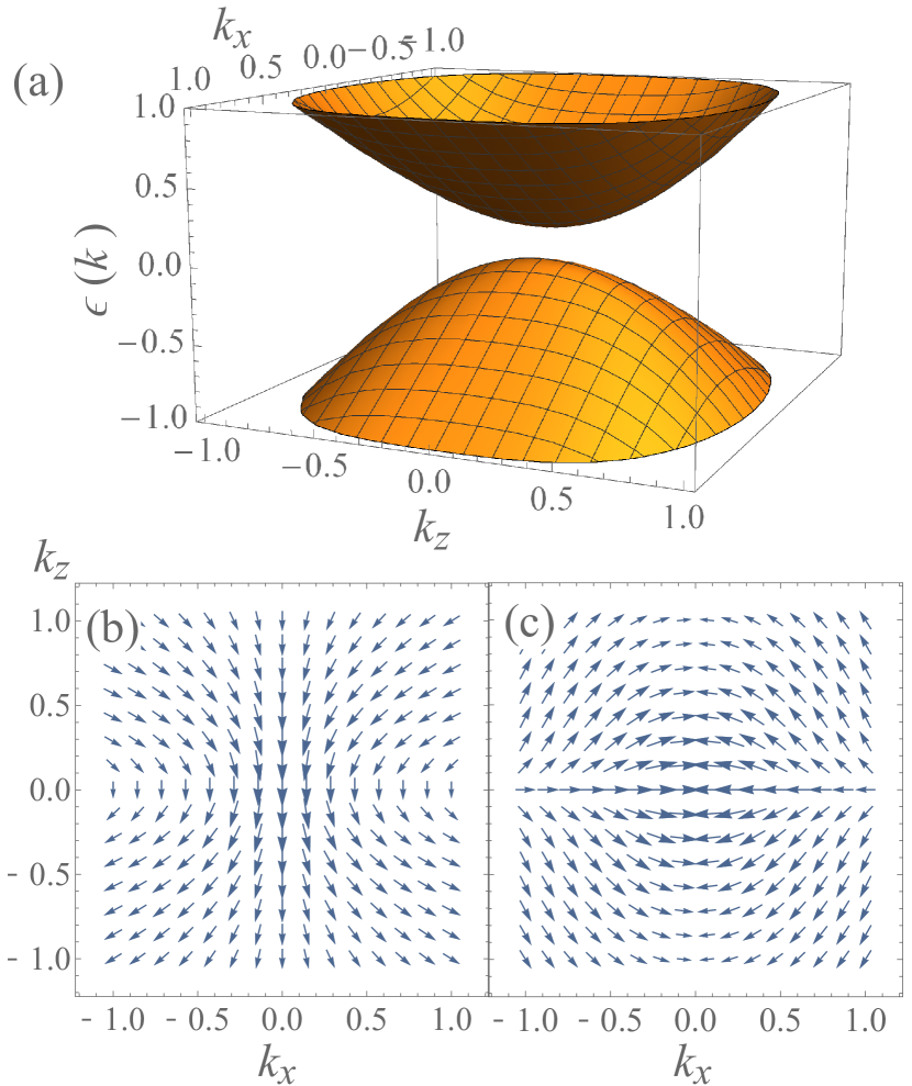
Figure 3: Band structure and Berry curvature distribution in the gapped Hamiltonian $H_{g}$. (a) The band structure, (b) Berry curvature distribution in the $k_{y}=0$ plane, and (c) distribution of $\bm{W}_{+}(\bm{k})$. The results are for $m=1/3$.

When $m^{2}=0$, i.e., at the critical point Yang et al. (2014), the anomaly-related current in the weak magnetic-field limit is obtained by substituting $m^{2}=0$ to Eqs. (36) and (37):

$$J_{\text{ano}}^{a}= \frac{\tau q^{4}}{(2\pi)^{2}}\left\{\frac{232}{693\mu^{\frac{3}{2}}}(\bm{B}\cdot\bm{E})B_{a}-\frac{2}{33\sqrt{3}\mu^{\frac{3}{2}}}Q_{z}(\bm{E},\bm{B})B_{a}\right.$$

$$\left.+\frac{77+240\mu}{10395\mu^{\frac{5}{2}}}(\bm{B}\cdot\bm{B})E_{a}+\frac{77-120\mu}{3465\sqrt{3}\mu^{\frac{5}{2}}}Q_{z}(\bm{B},\bm{B})E_{a}\right\},$$ (15a)

for $$a=x,y$$ and

$$J_{\text{ano}}^{z}= \frac{\tau q^{4}}{(2\pi)^{2}}\left\{-\frac{2(154\mu-975)}{27027\mu^{\frac{3}{2}}}(\bm{B}\cdot\bm{E})B_{a}\right.$$

$$\left.-\frac{39+308\mu}{9009\sqrt{3}\mu^{\frac{3}{2}}}Q_{z}(\bm{E},\bm{B})B_{a}+\frac{4}{117\mu^{\frac{1}{2}}}(\bm{B}\cdot\bm{B})E_{a}\right\}.$$ (15b)

We note that, when $\bm{B}\parallel\bm{E}$, only the current along the electric field direction survives with chemical potential dependence $\mu^{-3/2}$. Hence, when $\mu\to 0$, the current diverges with a different power from the Weyl case, $\propto\mu^{-2}$.

When $m^{2}>0$ and $\mu$ is close to the band edge, i.e., $\mu\sim m^{2}$, the current reads:

$$J_{\text{ano}}^{a}= \frac{\tau q^{4}}{(2\pi)^{2}}\left[\frac{4}{9m^{6}}\delta^{\frac{3}{2}}(\bm{B}\cdot\bm{E})B_{a}-\frac{2}{3\sqrt{3}m^{6}}\delta^{\frac{3}{2}}Q_{z}(\bm{E},\bm{B})B_{a}\right.$$

$$\left.+\frac{1}{9m^{8}}\delta^{\frac{3}{2}}(\bm{B}\cdot\bm{B})E_{a}+\frac{1}{3\sqrt{3}m^{8}}\delta^{\frac{3}{2}}Q_{z}(\bm{B},\bm{B})E_{a}\right],$$ (16a)

for $$a=x,y$$ and

$$J_{\text{ano}}^{z}= \frac{\tau q^{4}}{5\pi^{2}m^{8}}\left[\frac{2}{3}\delta^{\frac{5}{2}}(\bm{B}\cdot\bm{E})B_{z}-\frac{1}{\sqrt{3}}\delta^{\frac{5}{2}}Q_{z}(\bm{E},\bm{B})B_{z}\right.$$

$$\left.+\frac{4}{7}\delta^{\frac{7}{2}}(\bm{B}\cdot\bm{B})E_{z}\right],$$ (16b)

for $\delta\equiv\mu-m^{2}\geq 0$ and zero otherwise. Therefore, a finite anomaly-related current appears when $\delta>0$. The critical behavior of the current is highly anisotropic reflecting the symmetry of the Hamiltonian; it increases by $\delta^{\frac{3}{2}}$ for the current along $x$ and $y$. For the $z$ axis, in general, the current is proportional to $\delta^{\frac{5}{2}}$ for the current along $z$ axis. However, when $\bm{B}$ and $\bm{E}$ are both parallel to the $z$ axis, the first two terms in Eq. (16b) cancels, and the leading order becomes $\delta^{\frac{7}{2}}$. When $\delta<0$, on the other hand, the Fermi level is in the band gap, and therefore, the current is zero.

The result for $\bm{J}_{\text{ano}}$ for $\mu\gg m^{2}$ is the same as in Eq. (12) for $J_{\text{ano}}^{x}$ and $J_{\text{ano}}^{y}$. For $J_{\text{ano}}^{z}$, the term proportional to $m^{2}$ differs from the Weyl semimetal case:

$$J_{\text{ano}}^{z}=\frac{2\tau q^{4}}{(2\pi)^{2}} \left[-\frac{4(154\mu-975-351m^{2})}{27027\mu^{3/2}}(\bm{B}\cdot\bm{E})B_{z}\right.$$

$$\qquad-\frac{616\mu+78-1404m^{2}}{9009\sqrt{3}\mu^{3/2}}Q_{z}(\bm{E},\bm{B})B_{z}$$

$$\qquad\left.+\frac{616\mu-1404m^{2}}{9009\mu^{3/2}}(\bm{B}\cdot\bm{B})E_{z}\right].$$ (17)

Hence, the Berry-curvature-related current exists for arbitrary filling, even after the Weyl nodes vanish. The remnant of the Weyl nodes is found in the magnetoresistance even after the two Weyl nodes vanish by a pair annihilation.

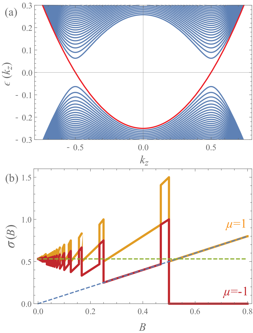
Figure 4: Electronic and transport properties under the strong magnetic field. (a) Landau levels of the Hamiltonian in Eq. (7). The result is for $m=1/2$ and when the magnetic field is applied along the $z$ axis. The Weyl nodes are located at $k_{z}=\pm 1/2$ when no magnetic field is applied. The red band corresponds to the chiral mode of Weyl Hamiltonian. (b) Magnetic field ($B$) dependence of electric current along the $z$ axis for $m=1/2$ and $\mu=1$ (yellow) and $-1$ (red). The green dashed lines indicates the conductivity in the limit $\sqrt{B}\ll\mu$ and the blue dashed line corresponds to the case in which only the chiral mode crosses the Fermi level. When $\mu=-1$, the conductivity goes to zero in the strong $B$ limit, as the Fermi level is below the bottom of the chiral mode.

IV Anomaly-related current under the strong field

IV.1 Two-node model

We next turn to the strong field limit $\omega_{c}\tau\gg 1$, where the Landau levels are formed. In this limit, the above semiclassical treatment of the magnetic field fails. Instead, we study the MR in this limit by considering the Boltzmann theory for the Landau levels Nielsen and Ninomiya (1983). We here consider the case in which the magnetic field is applied along the $z$ axis. In this case, the eigenenergies and the eigenstate wavefunctions of the Landau levels for the general Hamiltonian

$$H= \int\frac{dk^{3}}{(2\pi)^{3}}\psi^{\dagger}(k)\left\{\sigma_{1}k^{1}+\sigma_{2}k^{2}+\sigma_{3}f(k_{z})-\mu\sigma_{0}\right\}\psi(k).$$ (18)

is obtained by the same method used for Weyl Hamiltonian in Ref. Nielsen and Ninomiya (1983); here, $f(k_{z})$ is a general function of $k_{z}$. Assuming $qB_{z}>0$, the eigenenergy reads

$$\omega_{n}={\rm sgn}(n)\sqrt{2qB_{z}|n|+f^{2}(k_{z})},$$ (19)

where ${\rm sgn}(n)=1$ for $n\geq 0$ and $-1$ for $n<0$; most of the results remain the same when $qB<0$, except that ${\rm sgn}(n)=-1$ for $n=0$. Here, each Landau levels are $N_{\omega}=\lfloor\frac{qB_{z}}{2\pi}L^{2}\rfloor$ fold degenerate, where $L$ is the length along $x$ and $y$ directions and $\lfloor x\rfloor$ is the largest integer smaller than $x$. Therefore, when a Landau level crosses the Fermi level, the contribution of the level to the conductivity is expected to increase proportionally to $B$.

The Landau levels for the model in Eq. 7, i.e., $f(k_{z})=k_{z}^{2}-m^{2}$, is shown in Fig. 4. The mode that crosses the $\epsilon=0$ corresponds to the chiral modes of the Weyl Hamiltonian; $\omega_{0}(k_{z})=0$ when $k_{z}=\pm m$, which correspond to the positions of the Weyl nodes in absence of the magnetic field. When $\mu^{2}<2qB_{z}$, the chiral mode is the only mode that contributes to the electric conduction. In this limit, the Boltzmann theory within the relaxation-time approximation gives $j_{z}=\frac{q^{3}}{2\pi^{2}}\tau E_{z}B_{z},$ corresponds to the two Weyl nodes case in Ref. Nielsen and Ninomiya (1983); the result is independent of the group velocity of the electrons, which is a characteristic feature of the 1d systems.

When $\mu^{2}>2qB_{z}$, the result for $\mu^{2}<2qB_{z}$ is modified to include the contributions from different Landau levels:

$$j_{z}=\frac{q^{3}n_{b}}{2\pi^{2}}\tau E_{z}B_{z},$$ (20)

where $2n_{b}$ is the number of crossings between the Landau levels and the Fermi level with

$$n_{b}= \left[2\left\lfloor\frac{\mu^{2}}{2qB_{z}}\right\rfloor-\left\lfloor\frac{\mu^{2}-m^{2}}{2qB_{z}}\right\rfloor\Theta(\mu^{2}-m^{2})+\Theta(\mu+m)\right];$$ (21)

$\lfloor x\rfloor$ is the floor function. The last term in the square bracket comes from the chiral mode. The quantum oscillation comes from the product of $B_{z}$ and the floor functions in $n_{b}$. The result is plotted in Fig. 4(b). In the $\mu^{2}\gg m^{2},2qB_{z}$ limit, Eq. (21) is approximated as $n_{b}=(\mu^{2}+m^{2})/(2qB_{z})+{\cal O}(1)$, where the ${\cal O}(1)$ is related to the quantum oscillation. Therefore, the current becomes

$$j_{z}\sim\frac{q^{2}}{4\pi^{2}}\tau(\mu^{2}+m^{2})E_{z}.$$ (22)

Hence, in this limit, the magnetic field dependence of conductivity only shows up in the oscillation, which is the ${\cal O}(1)$ effect neglected in Eq. (22). In Fig. 4(b), this corresponds to the limit $B\to 0$, where the conductance converges to a finite value with oscillations around it. A notable difference in the structure of the quantum oscillation appears in the box-like structure of the conductivity at the right-end of the slope. This reflects the band structure of the two-node model, where the bottom of each Landau level is located at $k_{z}\neq 0$; this structure vanishes when $\mu\leq m^{2}$.

Another characteristic behavior appears in the strong field limit $\sqrt{qB}>|\mu|$. In this limit, the Landau levels with $|n|>0$ does not cross the Fermi level as the modes with $n>0$ ($n<0$) move to a higher (lower) energy. Therefore, the only Landau level that can cross the Fermi level is the $n=0$ mode. This is the case when $\mu>-m^{2}$ of which an example is shown in Fig. (4)(b) for $\mu=1$; this corresponds to the situation considered in Ref. Nielsen and Ninomiya (1983); Fukushima et al. (2008). For $\mu<-m^{2}$, however, the system shows a different behavior. In the two-node model in Eq. (7), the chiral mode exists only for $\mu\geq-m^{2}$. Therefore, when the Fermi level is $\mu<m^{2}$, the conductivity goes to zero in the strong field limit. These results are summarized in Fig. 1(a).

When the magnetic field is flipped, i.e., $qB<0$, the dispersion of the chiral mode also flips, i.e. $\omega_{0}=-(k_{z}^{2}-m^{2})$, and therefore, the equation for $n_{b}$ become

$$n_{b}= \left[2\left\lfloor\frac{\mu^{2}}{2qB_{z}}\right\rfloor-\left\lfloor\frac{\mu^{2}-m^{2}}{2qB_{z}}\right\rfloor\Theta(\mu^{2}-m^{2})-\Theta(\mu+m)\right].$$ (23)

Hence, in this case, the negative magnetoresistance in the strong-field limit appears only when $\mu<m^{2}$, in the opposite to the $qB>0$ cases.

IV.2 Near critical point

A similar argument also holds for the model in Eq. (14), when the system is near the critical point which the two Weyl nodes appear from a band touching. In this case, the current reads:

$$j_{z}= \frac{q^{3}}{2\pi^{2}}\tau E_{z}B_{z}\left[\left\lfloor\frac{\mu^{2}-m^{4}}{2qB_{z}}\right\rfloor\Theta(\mu^{2}-m^{4})+\Theta(\mu-m^{2})\right].$$ (24)

Most of the arguments above also apply to this case: when $\mu\gg m,qB$, the conductivity is $\sigma_{zz}=\frac{q^{2}\tau}{4\pi^{2}}(\mu^{2}-m^{4})+{\cal O}(1)$ where the quantum oscillation is included in the ${\cal O}(1)$, and $\sigma_{zz}\propto B_{z}$ in the strong field limit when only the lowest Landau level crosses the Fermi level. A difference is that the chiral mode crosses the Fermi level only when $\mu>m^{2}$ for $qB>0$ ($\mu<-m^{2}$ for $qB<0$), in contrast to $\mu>-m^{2}$ ($\mu<m^{2}$) in the case with two Weyl nodes.

V Discussion

To conclude, we studied the magnetoresistance in the Weyl semimetals that are related to the chiral anomaly. In the semiclassical limit, using the Boltzmann theory approach, we derive a general formula for the ${\cal O}(B^{2}E)$ response in the weak-field limit which is related to the Berry curvature of the electronic bands. The result shows the anomaly-related current is proportional to the square of $W_{\bm{k}\alpha}^{a}$, as shown in Eq. (5); for longitudinal negative magnetoresistance, it always gives an additional current along the electric field direction, i.e., longitudinal negative magnetoresistance as $(W_{\bm{k}\alpha}^{a})^{2}\geq 0$. In the case of Weyl semimetals, this shows that the contribution from different Weyl nodes do not cancel each other even when the Fermi level is away from the Weyl nodes and all the nodes are enclosed in a single Fermi surface. By considering a model with two Weyl nodes, we explicitly show that the anomaly-related magnetoresistance exists even when multiple Weyl nodes share a Fermi surface. Moreover, we find that the anomaly-related MR decays smoothly with increasing chemical potential. Therefore, a similar magnitude of magnetoresistance is expected even when all nodes are in a pocket.

On the other hand, in the quantum limit where the Landau levels are well formed, the behavior of the conductivity is governed by the structure and the degeneracy of Landau levels. In the relatively weak field region where a large number of Landau levels cross the Fermi surface, we show that the conductivity is roughly independent of the magnetic field unlike the semiclassical case; the quantum oscillation appears as a small wiggle on top of the field-independent conductivity. The chiral magnetic effect studied in Ref. Fukushima et al. (2008) is evident in the conductivity only when the lowest Landau level (chiral mode) crosses the Fermi surface. In general, this depends on the details of the Hamiltonian and chemical potential. However, the chiral mode in Eq. (7) crosses the Fermi level for arbitrary $\mu>-m^{2}$ (if $qB>0$). Therefore, the contribution from the chiral mode may also appear even if the Fermi level is far away from the Weyl nodes.

These results show that, especially in the semiclassical region, the magnetoresistance related to the chiral anomaly is extremely robust regardless of the details of the Hamiltonian nor the position of the Fermi surface. Furthermore, in our analyses on the gapped model in Eq. (14) (see also Fig. (3)), we find that the magnetoresistance remains even after the Weyl nodes pair annihilates.

In regard to experiments, recent experiments on Dirac/Weyl semimetal candidates observe negative magnetoresistance. However, its relation to the anomaly-related magnetoresistance is still under debate. One of the concerns in these experiments was the location of the Fermi level; it is often far away from the Weyl nodes and a Fermi surface encloses multiple Weyl nodes. Our theory, however, shows that the magnetoresistance should remain finite even in such cases. This is consistent with the recent experiments in Cd₃As₂ Li et al. (2016b); Nishihaya et al. (2018).

Another point regarding the experiment is the existence of multiple pairs of Weyl nodes. The unconventional electromagnetic response related to Weyl fermions often cancels out when taking into account of the existence of multiple nodes. For the chiral anomaly studied here, in the semiclassical limit, the total contribution from all pairs of Weyl fermions can be calculated simply by summing the contribution from each pair. Furthermore, as discussed in Eq. (5), each pair always gives a negative contribution to the resistivity. Therefore, no cancellation takes place. For instance, in Cd₃As₂ Wang et al. (2013); Neupane et al. (2014), there are two Dirac nodes, i.e., two pairs of Weyl nodes which are degenerate. The total current induced by the chiral anomaly in this material is given by the sum of contributions from the two pairs.

A slightly complicated example of Weyl semimetal is the pyrochlore iridates, where a Weyl semimetal phase is expected in the vicinity of the phase boundary of metal-insulator transition Wan et al. (2011); Witczak-Krempa et al. (2013), which is realized by controlling the temperature Matsuhira et al. (2011), by applying magnetic field Ueda et al. (2015a); Tian et al. (2015), or by chemical substitution Ueda et al. (2015b). In this material, there are four pairs of Weyl nodes of which a pair resides on each $\langle 111\rangle$ direction; they are related by the cubic symmetry of the magnetically ordered phase. In this material, when the Fermi level is sufficiently above the Weyl nodes, all eight nodes are expected to be in the same Fermi surface. This is a situation where the above results on the two-node model do not directly apply. Furthermore, the anti-ferroic pattern of the position of the eight Weyl nodes generates a multipolar pattern of the Berry curvature in the momentum space, which may seem to cancel the anomaly-related phenomena. However, from the general argument on Eq. (5), we see that the cancellation does not occur as the anomaly-related current is proportional to the momentum integral of $|\bm{W}_{\bm{k}\alpha}|^{2}$ where $\bm{W}_{\bm{k}\alpha}$ is defined below Eq. (4).

Appendix A Pumping of charge between different electron/hole pockets by chiral anomaly

We here show that, in the semiclassical limit, the rate of charges pumped by the chiral anomaly is determined only by the total charge of Weyl nodes enclosed in the pocket, regardless of the Hamiltonian nor the shape of the pocket. We consider the case $\tau\to\infty$. In this case, the change of $n_{\bm{k}\alpha}$ become

$$\partial_{t}n_{\bm{k}\alpha}=-\left(1+q\bm{B}\cdot\bm{b}_{\bm{k}\alpha}\right)^{-1}$$

$$\times\left(q\bm{E}+q\bm{v}_{\bm{k}\alpha}\times\bm{B}+q^{2}(\bm{E}\cdot\bm{B})\bm{b}_{\bm{k}\alpha}\right)\cdot\nabla_{\bm{k}}n_{\bm{k}\alpha}.$$ (25)

Intuitively, the $q^{2}(\bm{E}\cdot\bm{B})\bm{b}_{\bm{k}\alpha}$ term in Eq. (25) represents the change of wavepacket momentum; it flows along the Berry curvature $\bm{b}_{\bm{k}\alpha}$. In the case of the Weyl Hamiltonian, this gives a current flowing outward from/inward to the Weyl node, as the Weyl nodes are source/sink of $\bm{b}_{\bm{k}\alpha}$; this violates the chiral-charge conservation, which is known as the chiral anomaly Nielsen and Ninomiya (1983); Son and Spivak (2013). In general Hamiltonian, the time derivative of electron number in the $i$th Fermi surface reads

$$\dot{N}^{(i)}_{\alpha}\equiv \int_{BZ^{(i)}}\frac{dk^{3}}{(2\pi)^{3}}\left(1+q\bm{B}\cdot\bm{b}_{\bm{k}\alpha}\right)\partial_{t}n_{\bm{k}\alpha},$$ (26)

$$= \int_{\partial V^{(i)}}\frac{dS}{(2\pi)^{3}}\bm{n}_{S}\cdot\left(q\bm{v}_{\bm{k}\alpha}\times\bm{B}+q^{2}(\bm{E}\cdot\bm{B})\bm{b}_{\bm{k}\alpha}\right),$$ (27)

$$= \frac{q^{2}}{(2\pi)^{3}}(\bm{E}\cdot\bm{B})C^{(i)}.$$ (28)

Here, $BZ^{(i)}$ is a part of the Brillouin zone that encloses the region inside the $i$th Fermi surface $V^{(i)}\subset BZ^{(i)}$, $\partial V^{(i)}$ is the Fermi surface of $V^{(i)}$, $\bm{n}_{S}$ is the unit vector perpendicular to the surface $dS$. From the first to the second equation, we used the Gauss law. In the second equation, the first term in the integrand is zero as $\bm{v}_{\bm{k}\alpha}\parallel\bm{n}_{S}$. Hence, $\dot{N}^{(i)}_{\alpha}$ is proportional to the total charge of Weyl nodes $C^{(i)}\equiv\int_{\partial V^{(i)}}dS\,(\bm{n}_{S}\cdot\bm{b}_{\bm{k}\alpha})$, i.e., the amount of charge pumped between different Fermi surfaces is related to the topological property of the Weyl nodes. Therefore, the above argument on the “breakdown” of the chiral-charge conservation generally holds for arbitrary Hamiltonian whenever $C^{(i)}$ is nonzero. This implies that the chiral anomaly remains robust in Weyl semimetals, as the key feature of the Weyl Hamiltonian that gives rise to the chiral anomaly is the topological charge defined by $\bm{b}_{\bm{k}\alpha}$; the chiral anomaly occurs whenever the nonzero $C^{(i)}$ exist inside the Fermi surface, regardless of the precise form of Hamiltonian, location of the Weyl nodes, nor how far the chemical potentials are from them.

Appendix B Sensitiveness of the magnetoresistance to the electron distribution

We demonstrate how the details of electron distribution affect the anomaly-related current. For this purpose, we consider the Weyl Hamiltonian

$$H_{W}=v\bm{\sigma}\cdot\bm{p},$$ (29)

where the sign of $v$ corresponds to the different chiralities of the Weyl electrons. For the electron distribution, we consider:

$$\delta n_{\bm{k}\alpha}= -q\tau\left\{1-q\bm{B}\cdot\bm{b}_{\bm{p}}+\left(q\bm{B}\cdot\bm{b}_{\bm{p}}\right)^{2}\right\}(\bm{E}\cdot\bm{v}_{\bm{p}})\;(n_{\bm{p}}^{0})^{\prime}$$

$$-q^{2}\left\{\tau_{int}-q\tau\bm{B}\cdot\bm{b}_{\bm{p}}\right\}(\bm{E}\cdot\bm{B})(\bm{b}_{\bm{p}}\cdot\bm{v}_{\bm{p}})\;(n_{\bm{p}}^{0})^{\prime}.$$ (30)

This is a slightly generalized version of the expansion of $\delta n_{\bm{k}\alpha}$ in Eq. (3); $\tau$ for one of the term is replaced by $\tau_{int}$; $\tau_{int}$ corresponds to the inter-node scattering considered in Ref. Son and Spivak, 2013. When $\tau_{int}=\tau$, the electron distribution corresponds to the relaxation time approximation considered in this work, and $\tau=0$ corresponds to the approximation employed in Ref. Son and Spivak (2013); in the later case, the electron distribution remains symmetric while it becomes asymmetric in the former case due to the electron acceleration by the external field. The two relaxation times are phenomenologically introduced to show how the result changes when different approximation for the relaxation time (or electron distribution) is used.

Using these results, the ${\cal O}(EB^{2})$ current reads

$$\bm{J}_{\text{ano}}=\frac{q^{3}|v|^{3}}{8\pi^{2}\mu^{2}}\left\{\left(\tau_{int}-\frac{8}{15}\tau\right)(\bm{E}\cdot\bm{B})\bm{B}+\frac{\tau}{15}(\bm{B}\cdot\bm{B})\bm{E}\right\}.$$ (31)

When $\tau=0$, the current is proportional to $(\bm{E}\cdot\bm{B})\bm{B}$, reproducing the result in Ref. Son and Spivak (2013). When $\tau>0$, the result shows another term proportional to $(\bm{B}\cdot\bm{B})\bm{E}$, which comes from the asymmetry of the electron distribution around the Fermi surface.

Appendix C Solution of anomaly-related current in two-node Hamiltonian

C.1 Solution of anomaly-related current for general $\mu$

We here present the general solution for the anomaly related nonlinear current in Eq. (4) for the Hamiltonian in Eq. (7). The calculation was performed by reducing the three-dimensional integral in Eq. (4) to the integral over the Fermi surface. For arbitrary $\mu$, we find the coefficients $\sigma_{i}^{a}$ reads (see Eq. (8) for the definition of $\sigma_{i}^{a}$):

$$\sigma_{1}^{a} =\left\{\begin{array}[]{ll}\frac{4\pi(m^{2}-|\mu|)^{\frac{1}{2}}}{10395}\left(\frac{32m^{10}}{|\mu|^{7}}+\frac{16m^{8}}{|\mu|^{6}}-\frac{186m^{6}}{|\mu|^{5}}-\frac{89m^{4}}{|\mu|^{4}}-\frac{643m^{2}}{|\mu|^{3}}+\frac{870}{|\mu|^{2}}\right)\\ \qquad+\frac{4\pi(m^{2}+|\mu|)^{\frac{1}{2}}}{10395}\left(-\frac{32m^{10}}{|\mu|^{7}}+\frac{16m^{8}}{|\mu|^{6}}+\frac{186m^{6}}{|\mu|^{5}}-\frac{89m^{4}}{|\mu|^{4}}+\frac{643m^{2}}{|\mu|^{3}}+\frac{870}{|\mu|^{2}}\right)&(|\mu|\leq m^{2})\\ \frac{4\pi(m^{2}+|\mu|)^{\frac{3}{2}}}{10395}\left(-\frac{32m^{8}}{|\mu|^{7}}+\frac{48m^{6}}{|\mu|^{6}}+\frac{138m^{4}}{|\mu|^{5}}-\frac{227m^{2}}{|\mu|^{4}}+\frac{870}{|\mu|^{3}}\right)&(|\mu|>m^{2})\end{array}\right.$$ (32d)

$$\sigma_{2}^{a} =\left\{\begin{array}[]{ll}\frac{2\pi(m^{2}-|\mu|)^{\frac{1}{2}}}{693\sqrt{3}}\left(\frac{32m^{10}}{|\mu|^{7}}+\frac{16m^{8}}{|\mu|^{6}}+\frac{12m^{6}}{|\mu|^{5}}+\frac{10m^{4}}{|\mu|^{4}}-\frac{49m^{2}}{|\mu|^{3}}-\frac{21}{|\mu|^{2}}\right)\\ \qquad+\frac{2\pi(m^{2}+|\mu|)^{\frac{1}{2}}}{693\sqrt{3}}\left(-\frac{32m^{10}}{|\mu|^{7}}+\frac{16m^{8}}{|\mu|^{6}}-\frac{12m^{6}}{|\mu|^{5}}+\frac{10m^{4}}{|\mu|^{4}}+\frac{49m^{2}}{|\mu|^{3}}-\frac{21}{|\mu|^{2}}\right)&(|\mu|\leq m^{2})\\ -\frac{2\pi}{693\sqrt{3}}(m^{2}+|\mu|)^{\frac{3}{2}}\left(\frac{32m^{8}}{|\mu|^{7}}-\frac{48m^{6}}{|\mu|^{6}}+\frac{60m^{4}}{|\mu|^{5}}-\frac{70m^{2}}{|\mu|^{4}}+\frac{21}{|\mu|^{3}}\right)&(|\mu|>m^{2})\end{array}\right.$$ (32h)

$$\sigma_{3}^{a} =\left\{\begin{array}[]{ll}\frac{\pi(m^{2}-|\mu|)^{\frac{1}{2}}}{10395}\left(-\frac{64m^{10}-352m^{8}}{|\mu|^{7}}-\frac{32m^{8}-176m^{6}}{|\mu|^{6}}+\frac{240m^{6}-330m^{4}}{|\mu|^{5}}+\frac{112m^{4}-121m^{2}}{|\mu|^{4}}-\frac{496m^{2}+77}{|\mu|^{3}}+\frac{240}{|\mu|^{2}}\right)\\ \qquad+\frac{\pi(m^{2}+|\mu|)^{\frac{1}{2}}}{10395}\left(\frac{64m^{10}-352m^{8}}{|\mu|^{7}}-\frac{32m^{8}-176m^{6}}{|\mu|^{6}}-\frac{240m^{6}-330m^{4}}{|\mu|^{5}}+\frac{112m^{4}-121m^{2}}{|\mu|^{4}}+\frac{496m^{2}+77}{|\mu|^{3}}+\frac{240}{|\mu|^{2}}\right)&(|\mu|\leq m^{2})\\ \frac{\pi}{10395}(m^{2}+|\mu|)^{\frac{3}{2}}\left(\frac{64m^{8}-352m^{6}}{|\mu|^{7}}-\frac{96m^{6}-528m^{4}}{|\mu|^{6}}-\frac{144m^{4}+198m^{2}}{|\mu|^{5}}+\frac{256m^{2}+77}{|\mu|^{4}}+\frac{240}{|\mu|^{3}}\right)&(|\mu|>m^{2})\end{array}\right.$$ (32l)

$$\sigma_{4}^{a} =\left\{\begin{array}[]{ll}\frac{\pi(m^{2}-|\mu|)^{\frac{1}{2}}}{3465\sqrt{3}}\left(\frac{32m^{10}+352m^{8}}{|\mu|^{7}}+\frac{16m^{8}+176m^{6}}{|\mu|^{6}}-\frac{120m^{6}+330m^{4}}{|\mu|^{5}}-\frac{56m^{4}+121m^{2}}{|\mu|^{4}}+\frac{248m^{2}-77}{|\mu|^{3}}-\frac{120}{|\mu|^{2}}\right)\\ \qquad+\frac{\pi(m^{2}+|\mu|)^{\frac{1}{2}}}{3465\sqrt{3}}\left(-\frac{32m^{10}+352m^{8}}{|\mu|^{7}}+\frac{16m^{8}+176m^{6}}{|\mu|^{6}}+\frac{120m^{6}+330m^{4}}{|\mu|^{5}}-\frac{56m^{4}+121m^{2}}{|\mu|^{4}}-\frac{248m^{2}-77}{|\mu|^{3}}-\frac{120}{|\mu|^{2}}\right)&(|\mu|\leq m^{2})\\ -\frac{\pi}{3465\sqrt{3}}(m^{2}+|\mu|)^{\frac{3}{2}}\left(\frac{32m^{8}+352m^{6}}{|\mu|^{7}}-\frac{48m^{6}+528m^{4}}{|\mu|^{6}}-\frac{72m^{4}-198m^{2}}{|\mu|^{5}}+\frac{128m^{2}-77}{|\mu|^{4}}+\frac{120}{|\mu|^{3}}\right)&(|\mu|>m^{2})\end{array}\right.$$ (32p)

for $a=x,y$ and

$$\sigma_{1}^{z} =\left\{\begin{array}[]{ll}\frac{8\pi}{135135}(m^{2}-|\mu|)^{\frac{1}{2}}\left(-\frac{192m^{12}-416m^{10}}{|\mu|^{7}}-\frac{96m^{10}-208m^{8}}{|\mu|^{6}}+\frac{500m^{8}+1014m^{6}}{|\mu|^{5}}+\frac{226m^{6}+559m^{4}}{|\mu|^{4}}\right.\\ \left.\qquad\qquad+\frac{162m^{4}-7072m^{2}}{|\mu|^{3}}-\frac{1370m^{2}-4875}{|\mu|^{2}}+\frac{770}{|\mu|}\right)\\ \qquad+\frac{8\pi}{135135}(m^{2}+|\mu|)^{\frac{1}{2}}\left(\frac{192m^{12}-416m^{10}}{|\mu|^{7}}-\frac{96m^{10}-208m^{8}}{|\mu|^{6}}-\frac{500m^{8}+1014m^{6}}{|\mu|^{5}}+\frac{226m^{6}+559m^{4}}{|\mu|^{4}}\right.\\ \left.\qquad\qquad-\frac{162m^{4}-7072m^{2}}{|\mu|^{3}}-\frac{1370m^{2}-4875}{|\mu|^{2}}-\frac{770}{|\mu|}\right)&(|\mu|\leq m^{2})\\ \frac{8\pi(m^{2}+|\mu|)^{\frac{5}{2}}}{135135}\left(\frac{192m^{8}-416m^{6}}{|\mu|^{7}}-\frac{480m^{6}-1040m^{4}}{|\mu|^{6}}+\frac{268m^{4}-2678m^{2}}{|\mu|^{5}}+\frac{170m^{2}+4875}{|\mu|^{4}}-\frac{770}{|\mu|^{3}}\right)&(|\mu|>m^{2})\end{array}\right.$$ (33f)

$$\sigma_{2}^{z} =\left\{\begin{array}[]{ll}-\frac{4\pi}{45045\sqrt{3}}(m^{2}-|\mu|)^{\frac{1}{2}}\left(\frac{384m^{12}+1664m^{10}}{|\mu|^{7}}+\frac{192m^{10}+832m^{8}}{|\mu|^{6}}-\frac{1000m^{8}+3666m^{6}}{|\mu|^{5}}-\frac{452m^{6}+1625m^{4}}{|\mu|^{4}}\right.\\ \left.\qquad\qquad-\frac{324m^{4}-2600m^{2}}{|\mu|^{3}}+\frac{2740m^{2}+195}{|\mu|^{2}}-\frac{1540}{|\mu|}\right)\\ \qquad-\frac{4\pi}{45045\sqrt{3}}(m^{2}+|\mu|)^{\frac{1}{2}}\left(-\frac{384m^{12}+1664m^{10}}{|\mu|^{7}}+\frac{192m^{10}+832m^{8}}{|\mu|^{6}}+\frac{1000m^{8}+3666m^{6}}{|\mu|^{5}}-\frac{452m^{6}+1625m^{4}}{|\mu|^{4}}\right.\\ \left.\qquad\qquad+\frac{324m^{4}-2600m^{2}}{|\mu|^{3}}+\frac{2740m^{2}+195}{|\mu|^{2}}+\frac{1540}{|\mu|}\right)&(|\mu|\leq m^{2})\\ \frac{4\pi(m^{2}+|\mu|)^{\frac{5}{2}}}{45045\sqrt{3}}\left(\frac{384m^{8}+1664m^{6}}{|\mu|^{7}}-\frac{960m^{6}+4160m^{4}}{|\mu|^{6}}+\frac{536m^{4}+2990m^{2}}{|\mu|^{5}}+\frac{340m^{2}-195}{|\mu|^{4}}-\frac{1540}{|\mu|^{3}}\right)&(|\mu|>m^{2})\end{array}\right.$$ (33l)

$$\sigma_{3}^{z} =\left\{\begin{array}[]{ll}\frac{16\pi}{45045}(m^{2}-|\mu|)^{\frac{1}{2}}\left(\frac{96m^{12}}{|\mu|^{7}}+\frac{48m^{10}}{|\mu|^{6}}-\frac{250m^{8}}{|\mu|^{5}}-\frac{113m^{6}}{|\mu|^{4}}-\frac{81m^{4}}{|\mu|^{3}}+\frac{685m^{2}}{|\mu|^{2}}-\frac{385}{|\mu|}\right)\\ \qquad+\frac{16\pi}{45045}(m^{2}+|\mu|)^{\frac{1}{2}}\left(-\frac{96m^{12}}{|\mu|^{7}}+\frac{48m^{10}}{|\mu|^{6}}+\frac{250m^{8}}{|\mu|^{5}}-\frac{113m^{6}}{|\mu|^{4}}+\frac{81m^{4}}{|\mu|^{3}}+\frac{685m^{2}}{|\mu|^{2}}+\frac{385}{|\mu|}\right)&(|\mu|\leq m^{2})\\ \frac{16\pi(m^{2}+|\mu|)^{\frac{7}{2}}}{45045}\left(-\frac{96m^{6}}{|\mu|^{7}}+\frac{336m^{4}}{|\mu|^{6}}-\frac{470m^{2}}{|\mu|^{5}}+\frac{385}{|\mu|^{4}}\right)&(|\mu|>m^{2})\end{array}\right.$$ (33p)

The results are the same for $\mu<0$ and $\mu>0$, as $\bm{W}_{\bm{k}+}=-\bm{W}_{\bm{k}-}$ and the current is proportional to the square of $\bm{W}_{\bm{k}\pm}$, where $+$ and $-$ are respectively the conduction and valence bands of the Weyl node. We, however, note that the results of the Boltzmann theory are invalid when the Fermi level is close to the node, i.e., $|\mu|\lesssim q\tau|\bm{E}|$. This is a consequence of the band crossing, which its effect is not fully taken into account in the Boltzmann theory. The asymptotic form of $J^{a}_{\text{ano}}$ shown in the main text is calculated from these analytic solutions.

C.2 Anomaly-related current around $\mu\sim m^{2}$

In the Hamiltonian in Eq. (7), the two Weyl nodes are separated by a saddle point at $\bm{k}=\bm{0}$ and $\mu=m^{2}$, below which there exist two Fermi surfaces each contains a Weyl node and the two surfaces merge above. We here investigate how the two regions of $\mu$ connect at $\mu=m^{2}$. An explicit calculation shows $\sigma_{i}^{a}$ is a $C_{1}$ class function at $\mu=m^{2}$ for $a=x,y$ and $C_{2}$ class for $\sigma_{i}^{z}$ with an exception of $\sigma_{3}^{z}$ ($C_{3}$ class).

By substituting $\mu$ by $\delta\equiv m^{2}-\mu$ and expanding $\sigma_{i}^{a}$, we find

$$\sigma_{1}^{a} =\frac{\sqrt{2}\pi}{m^{3}}\left\{\frac{6376}{10395}-\frac{14866}{10395}\frac{\delta}{m^{2}}\right\}-\frac{4\pi}{9m^{3}}\left|\frac{\delta}{m^{2}}\right|^{\frac{3}{2}}\Theta(-\delta)$$ (34a)

$$\sigma_{2}^{a} =\frac{\sqrt{2}\pi}{\sqrt{3}m^{3}}\left\{\frac{20}{693}+\frac{13}{99}\frac{\delta}{m^{2}}\right\}+\frac{2\pi}{3\sqrt{3}m^{3}}\left|\frac{\delta}{m^{2}}\right|^{\frac{3}{2}}\Theta(-\delta)$$ (34b)

$$\sigma_{3}^{a} =\frac{\sqrt{2}\pi}{m^{3}}\left\{\frac{22+128m^{2}}{2079m^{2}}+\frac{77-2624m^{2}}{2079m^{2}}\frac{\delta}{m^{2}}\right\}$$

$$\qquad\qquad+\frac{\pi}{9m^{5}}\left|\frac{\delta}{m^{2}}\right|^{\frac{3}{2}}\Theta(-\delta)$$ (34c)

$$\sigma_{4}^{a} =\frac{\sqrt{2}\pi}{\sqrt{3}m^{3}}\left\{\frac{22-64m^{2}}{693m^{2}}+\frac{77+1312m^{2}}{6930m^{2}}\frac{\delta}{m^{2}}\right\}$$

$$\qquad\qquad+\frac{\pi}{3\sqrt{3}m^{5}}\left|\frac{\delta}{m^{2}}\right|^{\frac{3}{2}}\Theta(-\delta)$$ (34d)

for $a=x,y$ and

$$\sigma_{1}^{z} =-\frac{\sqrt{2}\pi}{m}\left\{\frac{19840m^{2}-90272}{135135m^{2}}+\frac{189176-33632m^{2}}{135135m^{2}}\left(\frac{\delta}{m^{2}}\right)+\frac{51588m^{2}-265499}{135135m^{2}}\left(\frac{\delta}{m^{2}}\right)^{2}\right\}+\frac{8\pi}{15m^{3}}\left|\frac{\delta}{m^{2}}\right|^{\frac{5}{2}}\Theta(-\delta)$$ (35a)

$$\sigma_{2}^{z} =-\frac{\sqrt{2}\pi}{\sqrt{3}m}\left\{\frac{39680m^{2}-9568}{90090m^{2}}+\frac{15496-67264m^{2}}{90090m^{2}}\left(\frac{\delta}{m^{2}}\right)+\frac{103176m^{2}-38389}{90090m^{2}}\left(\frac{\delta}{m^{2}}\right)^{2}\right\}-\frac{4\pi}{5\sqrt{3}m^{3}}\left|\frac{\delta}{m^{2}}\right|^{\frac{5}{2}}\Theta(-\delta)$$ (35b)

$$\sigma_{3}^{z} =\frac{\sqrt{2}\pi}{m}\left\{\frac{3968}{9009}-\frac{33632}{45045}\frac{\delta}{m^{2}}+\frac{5732}{5005}\left(\frac{\delta}{m^{2}}\right)^{2}-\frac{9137}{6435}\left(\frac{\delta}{m^{2}}\right)^{3}\right\}+\frac{16\pi}{35m}\left|\frac{\delta}{m^{2}}\right|^{\frac{7}{2}}\Theta(-\delta).$$ (35c)

These results show that a singular behavior appears at $\mu=m^{2}$, where the derivatives of $\bm{J}_{\text{ano}}$ with respect to $\mu$ diverges; the second derivative diverges for $J_{\text{ano}}^{x}$ and $J_{\text{ano}}^{y}$, while the third derivative diverges for $J_{\text{ano}}^{z}$.

Appendix D Magnetoresistance of the gapped model

We here present the general solution for the nonlinear current in Eq. (4) for the Hamiltonian in Eq. (14). By the same procedure with that of the Weyl semimetal case, we find the coefficients $\sigma_{i}^{a}$ are:

$$\sigma_{1}^{a} =\frac{4\pi(\mu-m^{2})^{\frac{3}{2}}}{10395}\left(-\frac{32m^{8}}{\mu^{7}}-\frac{48m^{6}}{\mu^{6}}+\frac{138m^{4}}{\mu^{5}}+\frac{227m^{2}}{\mu^{4}}+\frac{870}{\mu^{3}}\right)$$ (36a)

$$\sigma_{2}^{a} =-\frac{2\pi(\mu-m^{2})^{\frac{3}{2}}}{693\sqrt{3}}\left(\frac{32m^{8}}{\mu^{7}}+\frac{48m^{6}}{\mu^{6}}+\frac{60m^{4}}{\mu^{5}}+\frac{70m^{2}}{\mu^{4}}+\frac{21}{\mu^{3}}\right)$$ (36b)

$$\sigma_{3}^{a} =\frac{\pi(\mu-m^{2})^{\frac{3}{2}}}{10395}\left(\frac{64m^{8}+352m^{6}}{\mu^{7}}+\frac{96m^{6}+528m^{4}}{\mu^{6}}-\frac{144m^{4}-198m^{2}}{\mu^{5}}-\frac{256m^{2}-77}{\mu^{4}}+\frac{240}{\mu^{3}}\right)$$ (36c)

$$\sigma_{4}^{a} =-\frac{\pi(\mu-m^{2})^{\frac{3}{2}}}{3465\sqrt{3}}\left(\frac{32m^{8}-352m^{6}}{\mu^{7}}+\frac{48m^{6}-528m^{4}}{\mu^{6}}-\frac{72m^{4}+198m^{2}}{\mu^{5}}-\frac{128m^{2}+77}{\mu^{4}}+\frac{120}{\mu^{3}}\right)$$ (36d)

for $a=x,y$ and

$$\sigma_{1}^{z} =-\frac{8\pi(\mu-m^{2})^{\frac{5}{2}}}{135135}\left(-\frac{192m^{8}+416m^{6}}{\mu^{7}}-\frac{480m^{6}+1040m^{4}}{\mu^{6}}-\frac{268m^{4}+2678m^{2}}{\mu^{5}}+\frac{170m^{2}-4875}{\mu^{4}}+\frac{770}{\mu^{3}}\right),$$ (37a)

$$\sigma_{2}^{z} =-\frac{4\pi(\mu-m^{2})^{\frac{5}{2}}}{45045\sqrt{3}}\left(-\frac{384m^{8}-1664m^{6}}{\mu^{7}}-\frac{960m^{6}-4160m^{4}}{\mu^{6}}-\frac{536m^{4}-2990m^{2}}{\mu^{5}}+\frac{340m^{2}+195}{\mu^{4}}+\frac{1540}{\mu^{3}}\right),$$ (37b)

$$\sigma_{3}^{z} =\frac{16\pi(\mu-m^{2})^{\frac{7}{2}}}{45045}\left(\frac{96m^{6}}{\mu^{7}}+\frac{336m^{4}}{\mu^{6}}+\frac{470m^{2}}{\mu^{5}}+\frac{385}{\mu^{4}}\right).$$ (37c)

Further analysis of the above results is presented in the last part of the weak magnetic field section in Results.

References

- Fujikawa and Suzuki (2004) Kazuo Fujikawa and Hiroshi Suzuki, Path integrals and quantum anomalies (Oxford Science Publications, 2004).
- Fukuda and Miyamoto (1949) H. Fukuda and Y. Miyamoto, “On the -decay of neutral meson,” Prog. Theor. Phys. 4, 235 (1949).
- Fukuda et al. (1949a) H. Fukuda, Y. Miyamoto, T. Miyajima, and S. Tomonaga, “Application of Pauli’s regulator to the -decay of neutrettos,” Prog. Theor. Phys. 4, 385 (1949a).
- Fukuda et al. (1949b) H. Fukuda, Y. Miyamoto, T. Miyazima, S. Tomonaga, S. Oneda, S. Ozaki, and S. Sasaki, “Applicability of Pauli’s regulator to the -decay of neutrettos,” Progress of Theoretical Physics 4, 477–484 (1949b).
- Steinberger (1949) J. Steinberger, “On the use of subtraction fields and the lifetimes of some types of meson decay,” Phys. Rev. 76, 1180–1186 (1949).
- Vilenkin (1980) Alexander Vilenkin, “Equilibrium parity-violating current in a magnetic field,” Phys. Rev. D 22, 3080–3084 (1980).
- Nielsen and Ninomiya (1983) H.B. Nielsen and Masao Ninomiya, “The Adler-Bell-Jackiw anomaly and Weyl fermions in a crystal,” Physics Letters B 130, 389 – 396 (1983).
- Son and Spivak (2013) D. T. Son and B. Z. Spivak, “Chiral anomaly and classical negative magnetoresistance of Weyl metals,” Phys. Rev. B 88, 104412 (2013).
- Fang et al. (2003) Zhong Fang, Naoto Nagaosa, Kei S. Takahashi, Atsushi Asamitsu, Roland Mathieu, Takeshi Ogasawara, Hiroyuki Yamada, Masashi Kawasaki, Yoshinori Tokura, and Kiyoyuki Terakura, “The anomalous Hall effect and magnetic monopoles in momentum space,” Science 302, 92–95 (2003).
- Herring (1937) Conyers Herring, “Accidental degeneracy in the energy bands of crystals,” Phys. Rev. 52, 365–373 (1937).
- Murakami (2007) Shuichi Murakami, “Phase transition between the quantum spin Hall and insulator phases in 3d: emergence of a topological gapless phase,” New Journal of Physics 9, 356 (2007).
- Burkov and Balents (2011) A. A. Burkov and Leon Balents, “Weyl semimetal in a topological insulator multilayer,” Phys. Rev. Lett. 107, 127205 (2011).
- Xu et al. (2011) Gang Xu, Hongming Weng, Zhijun Wang, Xi Dai, and Zhong Fang, “Chern semimetal and the quantized anomalous Hall effect in ,” Phys. Rev. Lett. 107, 186806 (2011).
- Wan et al. (2011) Xiangang Wan, Ari M. Turner, Ashvin Vishwanath, and Sergey Y. Savrasov, “Topological semimetal and Fermi-arc surface states in the electronic structure of pyrochlore iridates,” Phys. Rev. B 83, 205101 (2011).
- Liu et al. (2014) Z. K. Liu, B. Zhou, Y. Zhang, Z. J. Wang, H. M. Weng, D. Prabhakaran, S.-K. Mo, Z. X. Shen, Z. Fang, X. Dai, Z. Hussain, and Y. L. Chen, “Discovery of a three-dimensional topological Dirac semimetal, Na3Bi,” Science 343, 864–867 (2014).
- Neupane et al. (2014) Madhab Neupane, Su-Yang Xu, Raman Sankar, Nasser Alidoust, Guang Bian, Chang Liu, Ilya Belopolski, Tay-Rong Chang, Horng-Tay Jeng, Hsin Lin, Arun Bansil, Fangcheng Chou, and M. Zahid Hasan, “Observation of a three-dimensional topological Dirac semimetal phase in high-mobility Cd3As2,” Nature Communications 5, 3786 (2014).
- Lv et al. (2015) B. Q. Lv, H. M. Weng, B. B. Fu, X. P. Wang, H. Miao, J. Ma, P. Richard, X. C. Huang, L. X. Zhao, G. F. Chen, Z. Fang, X. Dai, T. Qian, and H. Ding, “Experimental discovery of Weyl semimetal TaAs,” Phys. Rev. X 5, 031013 (2015).
- Xu et al. (2015) Su-Yang Xu, Ilya Belopolski, Nasser Alidoust, Madhab Neupane, Guang Bian, Chenglong Zhang, Raman Sankar, Guoqing Chang, Zhujun Yuan, Chi-Cheng Lee, Shin-Ming Huang, Hao Zheng, Jie Ma, Daniel S. Sanchez, BaoKai Wang, Arun Bansil, Fangcheng Chou, Pavel P. Shibayev, Hsin Lin, Shuang Jia, and M. Zahid Hasan, “Discovery of a Weyl fermion semimetal and topological Fermi arcs,” Science 349, 613–617 (2015).
- Oka and Aoki (2009) Takashi Oka and Hideo Aoki, “Photovoltaic Hall effect in graphene,” Phys. Rev. B 79, 081406 (2009).
- Potter et al. (2014) Andrew C. Potter, Itamar Kimchi, and Ashvin Vishwanath, “Quantum oscillations from surface Fermi arcs in Weyl and Dirac semimetals,” Nature Communications 5, 5161 (2014).
- Moll et al. (2016) Philip J. W. Moll, Nityan L. Nair, Toni Helm, Andrew C. Potter, Itamar Kimchi, Ashvin Vishwanath, and James G. Analytis, “Transport evidence for fermi-arc-mediated chirality transfer in the Dirac semimetal Cd3As2,” Nature 535, 266 – 270 (2016).
- Taguchi et al. (2016) Katsuhisa Taguchi, Tatsushi Imaeda, Masatoshi Sato, and Yukio Tanaka, “Photovoltaic chiral magnetic effect in Weyl semimetals,” Phys. Rev. B 93, 201202 (2016).
- Ebihara et al. (2016) Shu Ebihara, Kenji Fukushima, and Takashi Oka, “Chiral pumping effect induced by rotating electric fields,” Phys. Rev. B 93, 155107 (2016).
- Chan et al. (2016) Ching-Kit Chan, Patrick A. Lee, Kenneth S. Burch, Jung Hoon Han, and Ying Ran, “When chiral photons meet chiral fermions: Photoinduced anomalous hall effects in Weyl semimetals,” Phys. Rev. Lett. 116, 026805 (2016).
- Ishizuka et al. (2016) Hiroaki Ishizuka, Tomoya Hayata, Masahito Ueda, and Naoto Nagaosa, “Emergent electromagnetic induction and adiabatic charge pumping in noncentrosymmetric Weyl semimetals,” Phys. Rev. Lett. 117, 216601 (2016).
- Wu et al. (2016) Liang Wu, S. Patankar, T. Morimoto, N. L. Nair, E. Thewalt, A. Little, J. G. Analytis, J. E. Moore, and J. Orenstein, “Giant anisotropic nonlinear optical response in transition metal monopnictide weyl semimetals,” Nature Physics 13, 350 (2016).
- Ishizuka et al. (2017) Hiroaki Ishizuka, Tomoya Hayata, Masahito Ueda, and Naoto Nagaosa, “Momentum-space electromagnetic induction in Weyl semimetals,” Phys. Rev. B 95, 245211 (2017).
- Chan et al. (2017) Ching-Kit Chan, Netanel H. Lindner, Gil Refael, and Patrick A. Lee, “Photocurrents in Weyl semimetals,” Phys. Rev. B 95, 041104 (2017).
- Ma et al. (2017) Qiong Ma, Su-Yang Xu, Ching-Kit Chan, Cheng-Long Zhang, Guoqing Chang, Yuxuan Lin, Weiwei Xie, Tomas Palacios, Hsin Lin, Shuang Jia, Patrick A. Lee, Pablo Jarillo-Herrero, and Nuh Gedik, “Direct optical detection of Weyl fermion chirality in a topological semimetal,” Nature Physics 13, 842 – 847 (2017).
- de Juan et al. (2017) Fernando de Juan, Adolfo G. Grushin, Takahiro Morimoto, and Joel E. Moore, “Quantized circular photogalvanic effect in Weyl semimetals,” Nature Communications 8, 15995 (2017).
- (31) Gavin B. Osterhoudt, Laura K. Diebel, Xu Yang, John Stanco, Xiangwei Huang, Bing Shen, Ni Ni, Philip Moll, Ying Ran, and Kenneth S. Burch, “Colossal photovoltaic effect driven by the singular Berry curvature in a weyl semimetal,” preprint , (arXiv:1712.04951).
- Zhang et al. (2018a) Yang Zhang, Yan Sun, and Binghai Yan, “Berry curvature dipole in Weyl semimetal materials: An ab initio study,” Phys. Rev. B 97, 041101 (2018a).
- Zhang et al. (2018b) Yang Zhang, Hiroaki Ishizuka, Jeroen van den Brink, Claudia Felser, Binghai Yan, and Naoto Nagaosa, “Photogalvanic effect in Weyl semimetals from first principles,” Phys. Rev. B 97, 241118 (2018b).
- Liu et al. (2013) Chao-Xing Liu, Peng Ye, and Xiao-Liang Qi, “Chiral gauge field and axial anomaly in a Weyl semimetal,” Phys. Rev. B 87, 235306 (2013).
- Guinea et al. (2009) F. Guinea, M. I. Katsnelson, and A. K. Geim, “Energy gaps and a zero-field quantum hall effect in graphene by strain engineering,” Nature Physics 6, 30 – 33 (2009).
- Levy et al. (2010) N. Levy, S. A. Burke, K. L. Meaker, M. Panlasigui, A. Zettl, F. Guinea, A. H. Castro Neto, and M. F. Crommie, “Strain-induced pseudo–magnetic fields greater than 300 tesla in graphene nanobubbles,” Science 329, 544–547 (2010).
- Chernodub et al. (2014) Maxim N. Chernodub, Alberto Cortijo, Adolfo G. Grushin, Karl Landsteiner, and María A. H. Vozmediano, “Condensed matter realization of the axial magnetic effect,” Phys. Rev. B 89, 081407 (2014).
- Cortijo et al. (2015) Alberto Cortijo, Yago Ferreirós, Karl Landsteiner, and María A. H. Vozmediano, “Elastic gauge fields in Weyl semimetals,” Phys. Rev. Lett. 115, 177202 (2015).
- Pikulin et al. (2016) D. I. Pikulin, Anffany Chen, and M. Franz, “Chiral anomaly from strain-induced gauge fields in Dirac and Weyl semimetals,” Phys. Rev. X 6, 041021 (2016).
- Sumiyoshi and Fujimoto (2016) Hiroaki Sumiyoshi and Satoshi Fujimoto, “Torsional chiral magnetic effect in a Weyl semimetal with a topological defect,” Phys. Rev. Lett. 116, 166601 (2016).
- Grushin et al. (2016) Adolfo G. Grushin, Jörn W. F. Venderbos, Ashvin Vishwanath, and Roni Ilan, “Inhomogeneous Weyl and Dirac semimetals: Transport in axial magnetic fields and Fermi arc surface states from pseudo-Landau levels,” Phys. Rev. X 6, 041046 (2016).
- Cortijo et al. (2016) Alberto Cortijo, Dmitri Kharzeev, Karl Landsteiner, and Maria A. H. Vozmediano, “Strain-induced chiral magnetic effect in Weyl semimetals,” Phys. Rev. B 94, 241405 (2016).
- Gorbar et al. (2017) E. V. Gorbar, V. A. Miransky, I. A. Shovkovy, and P. O. Sukhachov, “Pseudomagnetic helicons,” Phys. Rev. B 95, 115422 (2017).
- Tchoumakov et al. (2017) Serguei Tchoumakov, Marcello Civelli, and Mark O. Goerbig, “Magnetic description of the Fermi arc in type-I and type-II Weyl semimetals,” Phys. Rev. B 95, 125306 (2017).
- (45) Toshikaze Kariyado, “Counting pseudo landau levels in spatially modulated Dirac systems,” preprint (arXiv:1707.08601) .
- Fukushima et al. (2008) Kenji Fukushima, Dmitri E. Kharzeev, and Harmen J. Warringa, “Chiral magnetic effect,” Phys. Rev. D 78, 074033 (2008).
- Sekine et al. (2017) Akihiko Sekine, Dimitrie Culcer, and Allan H. MacDonald, “Quantum kinetic theory of the chiral anomaly,” Phys. Rev. B 96, 235134 (2017).
- Liang et al. (2014) Tian Liang, Quinn Gibson, Mazhar N. Ali, Minhao Liu, R. J. Cava, and N. P. Ong, “Ultrahigh mobility and giant magnetoresistance in the Dirac semimetal Cd3As2,” Nature Materials 14, 280 – 284 (2014).
- Huang et al. (2015) Xiaochun Huang, Lingxiao Zhao, Yujia Long, Peipei Wang, Dong Chen, Zhanhai Yang, Hui Liang, Mianqi Xue, Hongming Weng, Zhong Fang, Xi Dai, and Genfu Chen, “Observation of the chiral-anomaly-induced negative magnetoresistance in 3d Weyl semimetal TaAs,” Phys. Rev. X 5, 031023 (2015).
- Xiong et al. (2015) Jun Xiong, Satya K. Kushwaha, Tian Liang, Jason W. Krizan, Max Hirschberger, Wudi Wang, R. J. Cava, and N. P. Ong, “Evidence for the chiral anomaly in the Dirac semimetal Na3Bi,” Science 350, 413–416 (2015).
- Li et al. (2016a) Qiang Li, Dmitri E. Kharzeev, Cheng Zhang, Yuan Huang, I. Pletikosito, A. V. Fedorov, R. D. Zhong, J. A. Schneeloch, G. D. Gu, and T. Valla, “Chiral magnetic effect in ZrTe5,” Nature Physics 12, 550 (2016a).
- Zhang et al. (2016) Cheng-Long Zhang, Su-Yang Xu, Ilya Belopolski, Zhujun Yuan, Ziquan Lin, Bingbing Tong, Guang Bian, Nasser Alidoust, Chi-Cheng Lee, Shin-Ming Huang, Tay-Rong Chang, Guoqing Chang, Chuang-Han Hsu, Horng-Tay Jeng, Madhab Neupane, Daniel S. Sanchez, Hao Zheng, Junfeng Wang, Hsin Lin, Chi Zhang, Hai-Zhou Lu, Shun-Qing Shen, Titus Neupert, M. Zahid Hasan, and Shuang Jia, “Signatures of the Adler-Bell-Jackiw chiral anomaly in a Weyl fermion semimetal,” Nature Communications 7, 10735 (2016).
- Hirschberger et al. (2016) Max Hirschberger, Satya Kushwaha, Zhijun Wang, Quinn Gibson, Sihang Liang, Carina Belvin, B. A. Bernevig, R. J. Cava, and N. P. Ong, “The chiral anomaly and thermopower of Weyl fermions in the half-Heusler GdPtBi,” Nature Materials 15, 1161 – 1165 (2016).
- Kuroda et al. (2017) K. Kuroda, T. Tomita, M.-T. Suzuki, C. Bareille, A. tuA Nugroho, P. Goswami, M. Ochi, M. Ikhlas, M. Nakayama, S. Akebi, R. Noguchi, R. Ishii, N. Inami, K. Ono, H. Kumigashira, A. Varykhalov, T. Muro, T. Koretsune, R. Arita, S. Shin, Takeshi Kondo, and S. Nakatsuji, “Evidence for magnetic Weyl fermions in a correlated metal,” Nature Materials 16, 1090 (2017).
- Niemann et al. (2017) Anna Corinna Niemann, Johannes Gooth, Shu-Chun Wu, Svenja Basler, Philip Sergelius, Ruben Huhne, Bernd Rellinghaus, Chandra Shekhar, Vicky Sus, Marcus Schmidt, Claudia Felser, Binghai Yan, and Kornelius Nielsch, “Chiral magnetoresistance in the Weyl semimetal NbP,” Scientific Reports 7, 43394 (2017).
- Zhang et al. (2017) Cheng Zhang, Enze Zhang, Weiyi Wang, Yanwen Liu, Zhi-Gang Chen, Shiheng Lu, Sihang Liang, Junzhi Cao, Xiang Yuan, Lei Tang, Qian Li, Chao Zhou, Teng Gu, Yizheng Wu, Jin Zou, and Faxian Xiu, “Room-temperature chiral charge pumping in Dirac semimetals,” Nature Communications 8, 13741 (2017).
- Liu et al. (2018) S. Liu, J. Lin, S. Kushwaha, R. J. Cava, and N. P. Ong, “Experimental tests of the chiral anomaly magnetoresistance in the Dirac-Weyl semimetals Na3Bi and GdPtBi,” preprint (arXiv:1802.01544) (2018).
- Li et al. (2016b) Hui Li, Hongtao He, Hai-Zhou Lu, Huachen Zhang, Hongchao Liu, Rong Ma, Zhiyong Fan, Shun-Qing Shen, and Jiannong Wang, “Negative magnetoresistance in Dirac semimetal Cd3As2,” Nature Communications 7, 10301 (2016b).
- Nishihaya et al. (2018) S. Nishihaya, M. Uchida, Y. Nakazawa, K. Akiba, M. Kriener, Y. Kozuka, A. Miyake, Y. Taguchi, M. Tokunaga, and M. Kawasaki, “Negative magnetoresistance suppressed through a topological phase transition in thin films,” Phys. Rev. B 97, 245103 (2018).
- Sundaram and Niu (1999) Ganesh Sundaram and Qian Niu, “Wave-packet dynamics in slowly perturbed crystals: Gradient corrections and Berry-phase effects,” Phys. Rev. B 59, 14915–14925 (1999).
- Xiao et al. (2010) Di Xiao, Ming-Che Chang, and Qian Niu, “Berry phase effects on electronic properties,” Rev. Mod. Phys. 82, 1959–2007 (2010).
- Kim et al. (2014) Ki-Seok Kim, Heon-Jung Kim, and M. Sasaki, “Boltzmann equation approach to anomalous transport in a Weyl metal,” Phys. Rev. B 89, 195137 (2014).
- Lundgren et al. (2014) Rex Lundgren, Pontus Laurell, and Gregory A. Fiete, “Thermoelectric properties of Weyl and Dirac semimetals,” Phys. Rev. B 90, 165115 (2014).
- Sharma et al. (2016) Girish Sharma, Pallab Goswami, and Sumanta Tewari, “Nernst and magnetothermal conductivity in a lattice model of Weyl fermions,” Phys. Rev. B 93, 035116 (2016).
- McCormick et al. (2017) Timothy M. McCormick, Robert C. McKay, and Nandini Trivedi, “Semiclassical theory of anomalous transport in type-ii topological Weyl semimetals,” Phys. Rev. B 96, 235116 (2017).
- Gao et al. (2017) Yang Gao, Shengyuan A. Yang, and Qian Niu, “Intrinsic relative magnetoconductivity of nonmagnetic metals,” Phys. Rev. B 95, 165135 (2017).
- Sharma et al. (2017) Girish Sharma, Pallab Goswami, and Sumanta Tewari, “Chiral anomaly and longitudinal magnetotransport in type-II Weyl semimetals,” Phys. Rev. B 96, 045112 (2017).
- Wei et al. (2018) Yi-Wen Wei, Chao-Kai Li, Jingshan Qi, and Ji Feng, “Magnetoconductivity of type-II Weyl semimetals,” Phys. Rev. B 97, 205131 (2018).
- Cortijo (2016) Alberto Cortijo, “Linear magnetochiral effect in Weyl semimetals,” Phys. Rev. B 94, 241105 (2016).
- Yang et al. (2014) Bohm-Jung Yang, Eun-Gook Moon, Hiroki Isobe, and Naoto Nagaosa, “Quantum criticality of topological phase transitions in three-dimensional interacting electronic systems,” Nature Physics 10, 774 – 778 (2014).
- Wang et al. (2013) Zhijun Wang, Hongming Weng, Quansheng Wu, Xi Dai, and Zhong Fang, “Three-dimensional Dirac semimetal and quantum transport in Cd3As2,” Phys. Rev. B 88, 125427 (2013).
- Witczak-Krempa et al. (2013) William Witczak-Krempa, Ara Go, and Yong Baek Kim, “Pyrochlore electrons under pressure, heat, and field: Shedding light on the iridates,” Phys. Rev. B 87, 155101 (2013).
- Matsuhira et al. (2011) Kazuyuki Matsuhira, Makoto Wakeshima, Yukio Hinatsu, and Seishi Takagi, “Metal-insulator transitions in pyrochlore oxides Ln2Ir2o7,” Journal of the Physical Society of Japan 80, 094701 (2011).
- Ueda et al. (2015a) K. Ueda, J. Fujioka, B.-J. Yang, J. Shiogai, A. Tsukazaki, S. Nakamura, S. Awaji, N. Nagaosa, and Y. Tokura, “Magnetic field-induced insulator-semimetal transition in a pyrochlore ,” Phys. Rev. Lett. 115, 056402 (2015a).
- Tian et al. (2015) Zhaoming Tian, Yoshimitsu Kohama, Takahiro Tomita, Hiroaki Ishizuka, Timothy H. Hsieh, Jun J. Ishikawa, Koichi Kindo, Leon Balents, and Satoru Nakatsuji, “Field-induced quantum metal-insulator transition in the pyrochlore iridate Nd2Ir2O7,” Nature Physics 12, 134 – 138 (2015).
- Ueda et al. (2015b) K. Ueda, J. Fujioka, C. Terakura, and Y. Tokura, “Pressure and magnetic field effects on metal-insulator transitions of bulk and domain wall states in pyrochlore iridates,” Phys. Rev. B 92, 121110 (2015b).