Disfluency Detection using Auto-Correlational Neural Networks

Abstract

In recent years, the natural language processing community has moved away from task-specific feature engineering, i.e., researchers discovering ad-hoc feature representations for various tasks, in favor of general-purpose methods that learn the input representation by themselves. However, state-of-the-art approaches to disfluency detection in spontaneous speech transcripts currently still depend on an array of hand-crafted features, and other representations derived from the output of pre-existing systems such as language models or dependency parsers. As an alternative, this paper proposes a simple yet effective model for automatic disfluency detection, called an auto-correlational neural network (ACNN). The model uses a convolutional neural network (CNN) and augments it with a new auto-correlation operator at the lowest layer that can capture the kinds of “rough copy” dependencies that are characteristic of repair disfluencies in speech. In experiments, the ACNN model outperforms the baseline CNN on a disfluency detection task with a 5% increase in f-score, which is close to the previous best result on this task.

1 Introduction

Disfluency informally refers to any interruptions in the normal flow of speech, including false starts, corrections, repetitions and filled pauses. Shriberg (1994) defines three distinct parts of a speech disfluency, referred to as the reparandum, interregnum and repair. As illustrated in Example 1, the reparandum to Boston is the part of the utterance that is replaced, the interregnum uh, I mean (which consists of a filled pause uh and a discouse marker I mean) is an optional part of a disfluent structure, and the repair to Denver replaces the reparandum. The fluent version is obtained by removing reparandum and interregnum words although disfluency detection models mainly deal with identifying and removing reparanda. The reason is that filled pauses and discourse markers belong to a closed set of words and phrases and are trivial to detect (Johnson and Charniak, 2004).

$$\begin{array}[]{l}\mbox{\it I want a flight~{}}\overbrace{\mbox{\it to Boston,}}^{\mbox{reparandum}}\\ \underbrace{\mbox{\it{}uh, I mean}}_{\mbox{interregnum}}\underbrace{\mbox{\it to Denver~{}}}_{\mbox{repair}}\mbox{\it on~{}Friday}\end{array}$$ (1)

In disfluent structures, the repair (e.g., to Denver) frequently seems to be a “rough copy” of the reparandum (e.g., to Boston). In other words, they incorporate the same or very similar words in roughly the same word order. In the Switchboard training set Godfrey and Holliman (1993), over $60\%$ of the words in the reparandum are exact copies of words in the repair. Thus, this similarity is strong evidence of a disfluency that can help the model detect reparanda (Charniak and Johnson, 2001; Johnson and Charniak, 2004). As a result, models which are able to detect “rough copies” are likely to perform well on this task.

Currently, state-of-the-art approaches to disfluency detection depend heavily on hand-crafted pattern match features, specifically designed to find such “rough copies” (Zayats et al., 2016; Jamshid Lou and Johnson, 2017). In contrast to many other sequence tagging tasks Plank et al. (2016); Yu et al. (2017), “vanilla” convolutional neural networks (CNNs) and long short-term memory (LSTM) models operating only on words or characters are surprisingly poor at disfluency detection Zayats et al. (2016). As such, the task of disfluency detection sits in opposition to the ongoing trend in NLP away from task-specific feature engineering — i.e., researchers discovering ad-hoc feature representations for various tasks — in favor of general-purpose methods that learn the input representation by themselves Collobert and Weston (2008).

In this paper, we hypothesize that LSTMs and CNNs cannot easily learn “rough copy” dependencies. We address this problem in the context of a CNN by introducing a novel auto-correlation operator. The resulting model, called an auto-correlational neural network (ACNN), is a generalization of a CNN with an auto-correlation operator at the lowest layer. Evaluating the ACNN in the context of disfluency detection, we show that introducing the auto-correlation operator increases f-score by 5% over a baseline CNN. Furthermore, the ACNN — operating only on word inputs — achieves results which are competitive with much more complex approaches relying on hand-crafted features and outputs from pre-existing systems such as language models or dependency parsers. In summary, the main contributions of this paper are:

• We introduce the auto-correlational neural network (ACNN), a generalization of a CNN incorporating auto-correlation operations,

• In the context of disfluency detection, we show that the ACNN captures important properties of speech repairs including “rough copy” dependencies, and

• Using the ACNN, we achieve competitive results for disfluency detection without relying on any hand-crafted features or other representations derived from the output of pre-existing systems.

2 Related Work

Approaches to disfluency detection task fall into three main categories: noisy channel models, parsing-based approaches and sequence tagging approaches. Noisy channel models (NCMs) (Johnson and Charniak, 2004; Johnson et al., 2004) use complex tree adjoining grammar (TAG) (Shieber and Schabes, 1990) based channel models to find the “rough copy” dependencies between words. The channel model uses the similarity between the reparandum and the repair to allocate higher probabilities to exact copy reparandum words. Using the probabilities of TAG channel model and a bigram language model (LM) derived from training data, the NCM generates $n$-best disfluency analyses for each sentence at test time. The analyses are then reranked using a language model which is sensitive to the global properties of the sentence, such as a syntactic parser based LM (Johnson and Charniak, 2004; Johnson et al., 2004). Some works have shown that rescoring the $n$-best analyses with external $n$-gram (Zwarts and Johnson, 2011) and deep learning LMs (Jamshid Lou and Johnson, 2017) trained on large speech and non-speech corpora, and using the LM scores along with other features (i.e. pattern match and NCM ones) into a MaxEnt reranker (Johnson et al., 2004) improves the performance of the baseline NCM, although this creates complex runtime dependencies.

Parsing-based approaches detect disfluencies while simultaneously identifying the syntactic structure of the sentence. Typically, this is achieved by augmenting a transition-based dependency parser with a new action to detect and remove the disfluent parts of the sentence and their dependencies from the stack (Rasooli and Tetreault, 2013; Honnibal and Johnson, 2014; Yoshikawa et al., 2016). Joint parsing and disfluency detection can compare favorably to pipelined approaches, but requires large annotated tree-banks containing both disfluent and syntatic structures for training.

Our proposed approach, based on an auto-correlational neural network (ACNN), belongs to the class of sequence tagging approaches. These approaches use classification techniques such as conditional random fields (Liu et al., 2006; Ostendorf and Hahn, 2013; Zayats et al., 2014; Ferguson et al., 2015), hidden Markov models (Liu et al., 2006; Schuler et al., 2010) and deep learning based models (Hough and Schlangen, 2015; Zayats et al., 2016) to label individual words as fluent or disfluent. In much of the previous work on sequence tagging approaches, improved performance has been gained by proposing increasingly complicated labeling schemes. In this case, a model with begin-inside-outside (BIO) style states which labels words as being inside or outside of edit region is usually used as the baseline sequence tagging model. Then in order to come up with different pattern matching lexical cues for repetition and correction disfluencies, they extend the baseline state space with new explicit repair states to consider the words at repair region, in addition to edit region (Ostendorf and Hahn, 2013; Zayats et al., 2014, 2016). A model which uses such labeling scheme may generate illegal label sequences at test time. As a solution, integer linear programming (ILP) constraints are applied to the output of classifier to avoid inconsistencies between neighboring labels (Georgila, 2009; Georgila et al., 2010; Zayats et al., 2016). This contrasts with our more straightforward approach, which directly labels words as being fluent or disfluent, and does not require any post-processing or annotation modifications.

The most similar work to ours is recent work by Zayats et al. (2016) that investigated the performance of a bidirectional long-short term memory network (BLSTM) for disfluency detection. Zayats et al. (2016) reported that a BLSTM operating only on words underperformed the same model augmented with hand-crafted pattern match features and POS tags by 7% in terms of f-score. In addition to lexically grounded features, some works incorporate prosodic information extracted from speech (Kahn et al., 2005; Ferguson et al., 2015; Tran et al., 2018). In this work, our primary motivation is to rectify the architectural limitations that prevent deep neural networks from automatically learning appropriate features from words alone. Therefore, our proposed model eschews manually engineered features and other representations derived from dependency parsers, language models or tree adjoining grammar transducers that are used to find “rough copy” dependencies. Instead, we aim to capture these kinds of dependencies automatically.

3 Convolutional and Auto-Correlational Networks

In this section, we introduce our proposed auto-correlation operator and the resulting auto-correlational neural network (ACNN) which is the focus of this work.

A convolutional or auto-correlational network computes a series of $h$ feature representations ${X}^{(0)},{X}^{(1)},\ldots,{X}^{(h)}$, where ${X}^{(0)}$ is the input data, ${X}^{(h)}$ is the final (output) representation, and each non-input representation ${X}^{(k)}$ for $k>0$, is computed from the preceding representation ${X}^{(k-1)}$ using a convolution or auto-correlation operation followed by an element-wise non-linear function.

Restricting our focus to convolutions in one dimension, as used in the context of language processing, each representation ${X}^{(k)}$ is a matrix of size $(n,m_{k})$, where $n$ is the number of words in the input and $m_{k}$ is the feature dimension of representation $k$, or equivalently it can be viewed as a sequence of $n$ row vectors ${X}^{(k)}=({\boldsymbol{x}}^{(k)}_{1},\ldots,{\boldsymbol{x}}^{(k)}_{n})$, where ${\boldsymbol{x}}^{(k)}_{t}$ is the row vector of length $m_{k}$ that represents the $t$th word at level $k$.

Consistent with the second interpretation, the input representation ${X}^{(0)}=({\boldsymbol{x}}^{(0)}_{1},\ldots,{\boldsymbol{x}}^{(0)}_{n})$ is a sequence of word embeddings, where $m_{0}$ is the length of the embedding vector and ${\boldsymbol{x}}^{(0)}_{t}$ is the word embedding for the $t$th word.

Each non-input representation ${X}^{(k)},k>0$ is formed by column-wise stacking the output of one or more convolution or auto-correlation operations applied to the preceding representation, and then applying an element-wise non-linear function. Formally, we define:

$${Y}^{(k)}= \left({F}^{(k,1)}({X}^{(k-1)});\ldots;{F}^{(k,m_{k})}({X}^{(k-1)})\right)$$

$${X}^{(k)}= {N}^{(k)}({Y}^{(k)})$$ (2)

where ${F}^{(k,u)}$ is the $u$th operator applied at layer $k$, and ${N}^{(k)}$ is the non-linear operation applied at layer $k$. Each operator ${F}^{(k,u)}$ (either convolution or auto-correlation) is a function from ${X}^{(k-1)}$, which is a matrix of size $(n,m_{k-1})$, to a vector of length $n$. A network that employs only convolution operators is a convolutional neural network (CNN). We call a network that utilizes a mixture of convolution and auto-correlation operators an auto-correlational neural network (ACNN). In our networks, the non-linear operation ${N}^{(k)}$ is always element-wise $\mathop{ReLU}$, except for the last layer, which uses a $\mathop{softmax}$ non-linearity.

3.1 Convolution Operator

A one-dimensional convolution operation maps an input matrix ${X}=({\boldsymbol{x}}_{1},\ldots,{\boldsymbol{x}}_{n})$, where each ${\boldsymbol{x}}_{t}$ is a row vector of length $m$, to an output vector ${\boldsymbol{y}}$ of length $n$. The convolution operation is defined by a convolutional kernel ${A}$, which is applied to a window of words to produce a new output representation, and kernel width parameters $\ell$ and $r$, which define the number of words to the left and right of the target word included in the convolutional window. For example, assuming appropriate input padding where necessary, element $y_{t}$ in the output vector ${\boldsymbol{y}}$ is computed as:

$$y_{t} = A\cdot X_{i:j}+{\boldsymbol{b}}$$ (3)

where

${A}$

is a learned convolutional kernel of dimension $(\ell+r,m)$,

$X_{i:j}$

is the sub-matrix formed by selecting rows $i$ to $j$ from matrix $X$,

$\cdot$

is the dot product (a sum over elementwise multiplications),

$i,j$

are given by $i=t-\ell$ and $j=t+r$, indicating the left and right extremities of the convolutional window effecting element $y_{t}$,

$\ell>0$

is the left kernel width, and

$r>0$

is right kernel width.

${\boldsymbol{b}}$

is a learned bias vector of dimension $n$,

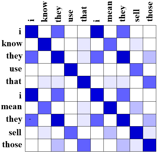
Figure 1: Cosine similarity between word embedding vectors learned by the ACNN model for the sentence “I know they use that I mean they sell those” (with disfluent words highlighted). In the figure, darker shades denote higher cosine values. “Rough copies” are clearly indicated by darkly shaded diagonals, which can be detected by our proposed auto-correlation operator.

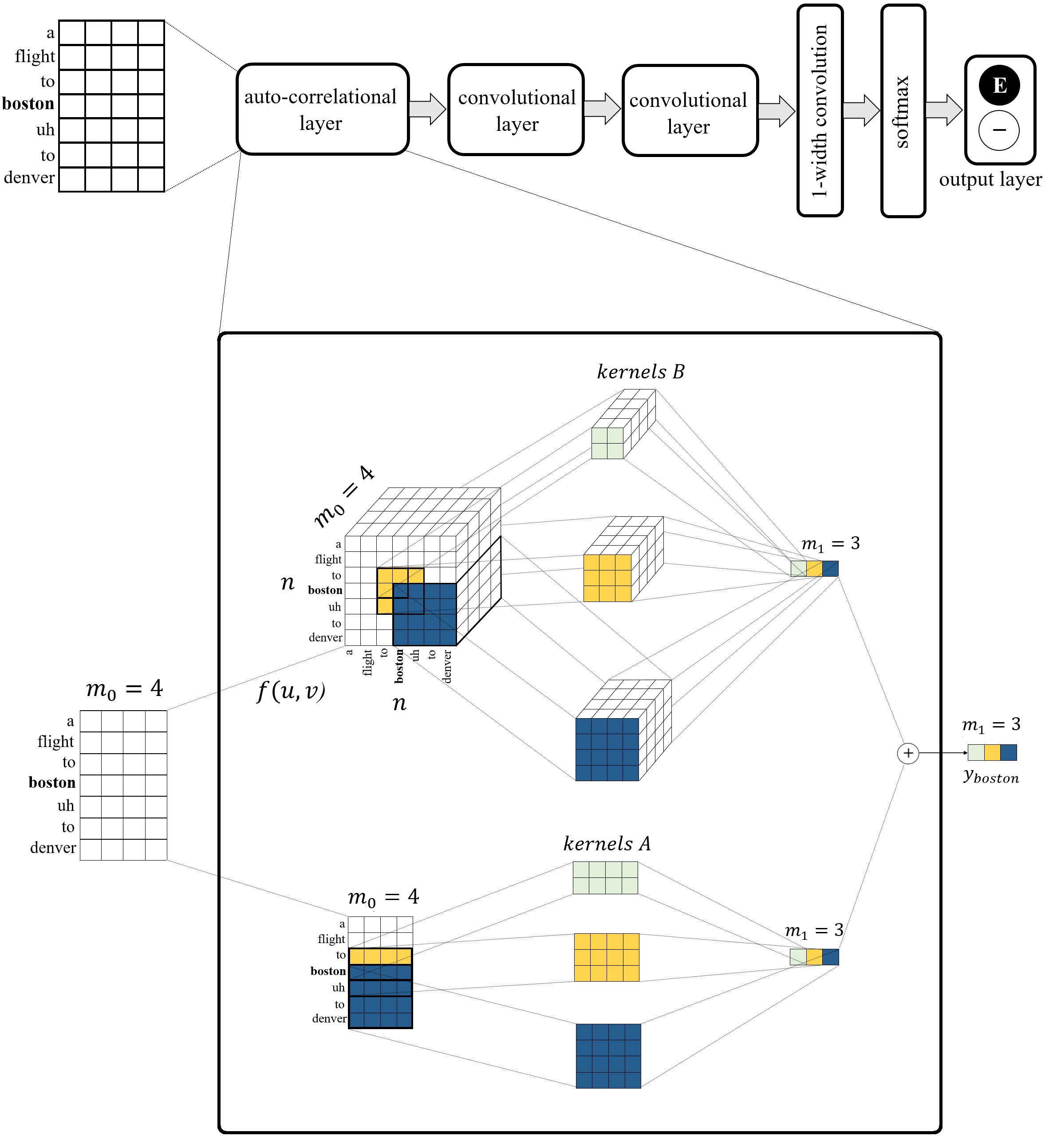
Figure 2: ACNN overview for labeling the target word “boston”. A patch of words is fed into an auto-correlational layer. At inset bottom, the given patch of words is convolved with 2D kernels $A$ of different sizes. At inset top, an auto-correlated tensor of size $(n,n,m_{0})$ is constructed by comparing each input vector ${\boldsymbol{u}}={\boldsymbol{x}}_{t}$ with the input vector ${\boldsymbol{v}}={\boldsymbol{x}}_{t^{\prime}}$ using a binary function $f({\boldsymbol{u}},{\boldsymbol{v}})$. The auto-correlated tensor is convolved with 3D kernels $B$ of different sizes. Each kernel group $A$ and $B$ outputs a matrix of size $(n,m_{1})$ (here, we depict only the row vector relating to the target word “boston”). These outputs are added element-wise to produce the feature representation that is passed to further convolutional layers, followed by a softmax layer. “E” = disfluent, “$\_$” = fluent and $m_{0}$ = embedding size.

3.2 Auto-Correlation Operator

The auto-correlational operator is a generalisation of the convolution operator:

$$y_{t} = A\cdot X_{i:j}+B\cdot\hat{X}_{i:j,i:j}+{\boldsymbol{b}}$$ (4)

where $y_{t}$, $A$, $X$, ${\boldsymbol{b}}$, $i$ and $j$ are as in the convolution operator, and

$\hat{X}$

is a tensor of size $(n,n,m)$ such that each vector $\hat{X}_{i,j,:}$ is given by $f({\boldsymbol{x}}_{i},{\boldsymbol{x}}_{j})$,

$f({\boldsymbol{u}},{\boldsymbol{v}})$

is a binary operation on vectors, such as the Hadamard or element-wise product (i.e., $f({\boldsymbol{u}},{\boldsymbol{v}})={\boldsymbol{u}}\circ{\boldsymbol{v}}$), and

$\hat{X}_{i:j,i:j}$

is the sub-tensor formed by selecting indices $i$ to $j$ from the first two dimensions of tensor $\hat{X}$,

${B}$

is a learned convolutional kernel of dimension $(\ell+r,\ell+r,m)$.

Unlike convolution operations, which are linear, the auto-correlation operator introduces second-order interaction terms through the tensor $\hat{X}$ (since it multiplies the vector representations for each pair of input words). This naturally encodes the similarity between input words when applied at level $k=1$ (or the co-activations of multiple CNN features, if applied at higher levels). As illustrated in Figure 1, blocks of similar words are indicative of “rough copies”. We provide an illustration of the auto-correlation operation in Figure 2.

4 Experiments

4.1 Switchboard Dataset

We evaluate the proposed ACNN model for disfluency detection on the Switchboard corpus of conversational speech Godfrey and Holliman (1993). Switchboard is the largest available corpus ($1.2\times 10^{6}$ tokens) where disfluencies are annotated according to Shriberg’s (1994) scheme:

[ reparandum + {interregnum} repair ]

where (+) is the interruption point marking the end of reparandum and {} indicate optional interregnum. We collapse this annotation to a binary classification scheme in which reparanda are labeled as disfluent and all other words as fluent. We disregard interregnum words as they are trivial to detect as discussed in Section 1.

Following Charniak and Johnson Charniak and Johnson (2001), we split the Switchboard corpus into training, dev and test set as follows: training data consists of all sw[23]$\ast$.dff files, dev training consists of all sw4[5-9]$\ast$.dff files and test data consists of all sw4[0-1]$\ast$.dff files. We lower-case all text and remove all partial words and punctuations from the training data to make our evaluation both harder and more realistic (Johnson and Charniak, 2004). Partial words are strong indicators of disfluency; however, speech recognition models never generate them in their outputs.

4.2 ACNN and CNN Baseline Models

We investigate two neural network models for disfluency detection; our proposed auto-correlational neural network (ACNN) and a convolutional neural network (CNN) baseline. The CNN baseline contains three convolutional operators (layers), followed by a width-1 convolution and a softmax output layer (to label each input word as either fluent or disfluent). The ACNN has the same general architecture as the baseline, except that we have replaced the first convolutional operator with an auto-correlation operator, as illustrated in Figure 2.

To ensure that equal effort was applied to the hyperparameter optimization of both models, we use randomized search Bergstra and Bengio (2012) to tune the optimization and architecture parameters separately for each model on the dev set, and to find an optimal stopping point for training. This results in different dimensions for each model. As indicated by Table 1, the resulting ACNN configuration has far fewer kernels at each layer than the CNN. However, as the auto-correlation kernels contain an additional dimension, both models have a similar number of parameters overall. Therefore, both models should have similar learning capacity except for their architectural differences (which is what we wish to investigate). Finally, we note that the resulting maximum right kernel width $r_{1}$ in the auto-correlational layer is 6. As illustrated in Figure 3, this is sufficient to capture almost all the “rough copies” in the Switchboard dataset (but could be increased for other datasets).

Configuration	CNN	ACNN
embedding dim	$290$	$290$
dropout rate	$0.51$	$0.53$
$L_{2}$ regularizer weight	$0.13$	$0.23$
$\#$kernels at each layer	$570$	$120$
$\#$kernel sizes at each layer	$3$	$2$
$\#$words at left context $\ell_{1}$	[0,1,4]	[5,3]
$\#$words at left context $\ell_{2}$	[1,2,3]	[4,2]
$\#$words at left context $\ell_{3}$	[0,1,2]	[3,2]
$\#$words at right context $r_{1}$	[1,1,4]	[6,3]
$\#$words at right context $r_{2}$	[1,2,4]	[5,3]
$\#$words at right context $r_{3}$	[1,2,3]	[4,2]
$\#$parameters	4.9M	4.9M

Table 1: Configuration of the CNN and ACNN models, where $\ell_{k}$ refers to the left kernel width at layer $k$, and $r_{k}$ refers to the right kernel width at layer $k$. Both models have a similar total number of parameters.

For the ACNN, we considered a range of possible binary functions $f({\boldsymbol{u}},{\boldsymbol{v}})$ to compare the input vector ${\boldsymbol{u}}={\boldsymbol{x}}_{t}$ with the input vector ${\boldsymbol{v}}={\boldsymbol{x}}_{t^{\prime}}$ in the auto-correlational layer. However, in initial experiments we found that the Hadamard or element-wise product (i.e. $f({\boldsymbol{u}},{\boldsymbol{v}})={\boldsymbol{u}}\circ{\boldsymbol{v}}$) achieved the best results. We also considered concatenating the outputs of kernels $A$ and $B$ in Equation 4, but we found that element-wise addition produced slightly better results on the dev set.

4.2.1 Implementation Details

In both models, we use $\mathop{ReLU}$ for the non-linear operation, all stride sizes are one word and there are no pooling operations. We randomly initialize the word embeddings and all weights of the model from a uniform distribution. The bias terms are initialized to be $1$. To reduce overfitting, we apply dropout Srivastava et al. (2014) to the input word embeddings and $L_{2}$ regularization to the weights of the width-1 convolutional layer. For parameter optimization, we use the Adam optimizer (Kingma and Ba, 2014) with a mini-batch size of $25$ and an initial learning rate of $0.001$.

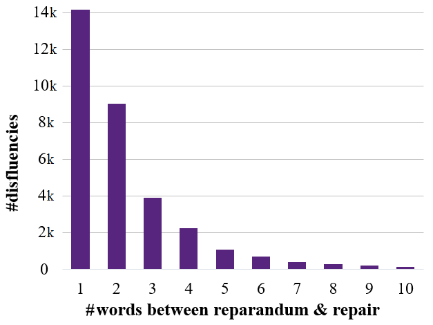
Figure 3: Distribution over the number of words in between the reparandum and the interregnum in the Switchboard training set (indicating the distance between “rough copies”).

5 Results

As in previous work (Johnson and Charniak, 2004), we evaluate our model using precision, recall and f-score, where true positives are the words in the edit region (i.e., the reparandum words). As Charniak and Johnson (2001) observed, only $6\%$ of words in the Switchboard corpus are disfluent, so accuracy is not a good measure of system performance. F-score, on the other hand, focuses more on detecting “edited” words, so it is more appropriate for highly skewed data.

Table 2 compares the dev set performance of the ACNN model against our baseline CNN, as well as the LSTM and BLSTM models proposed by Zayats et al. (2016) operating only on word inputs (i.e., without any disfluency pattern-match features). Our baseline CNN outperforms both the LSTM and the BLSTM, while the ACNN model clearly outperforms the baseline CNN, with a further 5% increase in f-score. In particular, the ACNN noticeably improves recall without degrading precision.

model	P	R	F
BLSTM (words)∗	$87.8$	$71.1$	$78.6$
LSTM (words)∗	$87.6$	$71.4$	$78.7$
CNN	$89.4$	$74.6$	$81.3$
ACNN	$\bf 90.0$	$\bf 82.8$	$\bf 86.2$

Table 2: Precision (P), recall (R) and f-score (F) on the dev set for the BLSTM and LSTM models using words alone from ^∗Zayats et al. (2016), as well as our baseline CNN and ACNN model.

To further investigate the differences between the two CNN-based models, we randomly select $100$ sentences containing disfluencies from the Switchboard dev set and categorize them according to Shriberg’s (1994) typology of speech repair disfluencies. Repetitions are repairs where the reparandum and repair portions of the disfluency are identical, while corrections are where the reparandum and repairs differ (so corrections are much harder to detect). Restarts are where the speaker abandons a sentence prefix, and starts a fresh sentence. As Table 3 shows, the ACNN model is better at detecting repetition and correction disfluencies than the CNN, especially for the more challenging correction disfluencies. On the other hand, the ACNN is no better than the baseline at detecting restarts, probably because the restart typically does not involve a rough copy dependency. Luckily restarts are much rarer than repetition and correction disfluencies.

model	Rep.	Cor.	Res.	All
CNN	$93.3$	$66.0$	$57.1$	$80.4$
ACNN	$97.5$	$80.0$	$57.1$	$88.9$

Table 3: F-scores for different types of disfluencies on a subset of the Switchboard dev set containing $140$ disfluent structures — including $85$ repetitions (Rep.), $51$ corrections (Cor.) and $4$ restarts (Res.).

We also repeated the analysis of (Zayats et al., 2014) on the dev data, so we can compare our models to their extended BLSTM model with a 17-state CRF output and hand-crafted features, including partial-word and POS tag features that enable it to capture some “rough copy” dependencies. As expected, the ACNN outperforms both the CNN and the extended BLSTM model, especially in the “Other” category that involve the non-repetition dependencies.

model	Rep.	Other	Either
CNN	$92.2$	$66.7$	$81.3$
BLSTM (17 states)∗	$94.1$	$66.7$	$85.8$
ACNN	$96.6$	$73.3$	$86.2$

Table 4: F-scores for different types of disfluencies for the CNN, ACNN and BLSTM (17 states) ^∗(Zayats et al., 2016) using the Switchboard dev set.

Finally, we compare the ACNN model to state-of-the-art methods from the literature, evaluated on the Switchboard test set. Table 5 shows that the ACNN model is competitive with recent models from the literature. The three models that score more highly than the ACNN all rely on hand-crafted features, additional information sources such as partial-word features (which would not be available in a realistic ASR application), or external resources such as dependency parsers and language models. The ACNN, on the other hand, only uses whole-word inputs and learns the “rough copy” dependencies between words without requiring any manual feature engineering.

model	P	R	F
Yoshikawa et al.(2016) $\bf\diamond$	$67.9$	$57.9$	$62.5$
Georgila et al. (2010)$~{}\bf\dagger$	$77.4$	$64.6$	$70.4$
Tran et al. (2018)$~{}\bf\otimes\star$	-	-	$77.5$
Kahn et al. (2005) $\bf\star$	-	-	$78.2$
Johnson et al. (2004) $\bf\wr$	$82.0$	$77.8$	$79.7$
Georgila (2009)$~{}\bf\dagger$	-	-	$80.1$
Johnson et al. (2004) $\bf\dagger\wr$	-	-	$81.0$
Rasooli et al. (2013) $\bf\diamond$	$85.1$	$77.9$	$81.4$
Zwarts et al. (2011) $\bf\Join\wr$	-	-	$83.8$
Qian et al. (2013) $\bf\Join$	-	-	$84.1$
Honnibal et al. (2014) $\bf\diamond$	-	-	$84.1$
ACNN	$\bf 89.5$	$\bf 80.0$	$\bf 84.5$
Ferguson et al. (2015) $\bf\star$	$90.0$	$81.2$	$85.4$
Zayats et al. (2016) $\bf\otimes\dagger$	$91.8$	$80.6$	$85.9$
Jamshid Lou et al. (2017) $\bf\Join\wr$	-	-	$86.8$

Table 5: Comparison of the ACNN model to the state-of-the-art methods on the Switchboard test set. The other models listed have used richer inputs and/or rely on the output of other systems, as well as pattern match features, as indicated by the following symbols: $\bf\diamond$ dependency parser, $\bf\dagger$ hand-crafted constraints/rules, $\bf\star$ prosodic cues, $\bf\wr$ tree adjoining grammar transducer, $\bf\Join$ refined/external language models and $\bf\otimes$ partial words. P = precision, R = recall and F = f-score.

5.1 Qualitative Analysis

We conduct an error analysis on the Switchboard dev set to characterize the disfluencies that the ACNN model can capture and those which are difficult for the model to detect. In the following examples, the highlighted words indicate ground truth disfluency labels and the underlined ones are the ACNN predictions.

1. But if you let them yeah if you let them in a million at a time it wouldn’t make that you know it wouldn’t make that big a bulge in the population
   

2. They’re handy uh they they come in handy at the most unusual times
   

3. My mechanics loved it because it was an old it was a sixty-five buick
   

4. Well I I I think we did I think we did learn some lessons that we weren’t uh we weren’t prepared for
   

5. Uh I have never even I have never even looked at one closely
   

6. But uh when I was when my kids were young I was teaching at a university
   

7. She said she’ll never put her child in a in a in a in a in a preschool
   

8. Well I think they’re at they’re they’ve come a long way
   

9. I I like a I saw the the the the tapes that were that were run of marion berry’s drug bust
   

10. But I know that in some I know in a lot of rural areas they’re not that good
    

According to examples 1-10, the ACNN detects repetition (e.g. 1, 5) and correction disfluencies (e.g. 3, 6, 10). It also captures complex structures where there are multiple or nested disfluencies (e.g. 2, 8) or stutter-like repetitions (e.g. 4, 7, 9).

1. My point was that there is for people who don’t want to do the military service it would be neat if there were an alternative $\ldots$
   

2. I believe from what I remember of the literature they gave uh if you fail I believe they give you one more chance
   

3. Kind of a coarse kind of test
   

4. So we could pour concrete and support it with a a nice firm four by four posts
   

5. But uh I’m afraid I’m I’m probably in the minority
   

6. Same thing same thing that the her kids had
   

7. Did you you framed it in uh on on you framed in new square footage
   

8. And and and there needs to be a line drawn somewhere at reasonable and proper
   

9. $\dots$ I think there’s a couple of levels of tests in terms of of drugs
   

10. See they have uh we have two the both c spans here

In some cases where repetitions are fluent, the model has incorrectly detected the first occurence of the word as disfluency (e.g. 13, 14, 15, 19). Moreover, when there is a long distance between reparandum and repair words (e.g. 11, 12), the model usually fails to detect the reparanda. In some sentences, the model is also unable to detect the disfluent words which result in ungrammatical sentences (e.g. 16, 17, 18, 20). In these examples, the undetected disfluencies “the”, “did”, “at” and “two the” cause the residual sentence to be ungrammatical.

We also discuss the types of disfluency captured by the ACNN model, but not by the baseline CNN. In the following examples, the ACNN predictions (underlined words) are the same as the ground truth disfluency labels (highlighted words). The bolded words indicate the CNN prediction of disfluencies.

1. Uh well I actually my dad’s my dad’s almost ninety
   

2. Not a man not a repair man but just a friend
   

3. we’re from a county we’re from the county they marched in
   

4. Now let’s now we’re done
   

5. And they’ve most of them have been pretty good
   

6. I do as far as uh as far as uh as far as immigration as a whole goes
   

7. No need to use this to play around with this space stuff anymore
   

8. We couldn’t survive in a in a juror in a trial system without a jury
   

9. You stay within your uh within your means
   

10. So we’re we’re part we’re actually part of MIT

The ACNN model has a generally better performance in detecting “rough copies” which are important indicator of repetition (e.g. 21, 29), correction (e.g. 22, 23, 24, 25, 27), and stutter-like (e.g. 26, 28, 30) disfluencies.

6 Conclusion

This paper presents a simple new model for disfluency detection in spontaneous speech transcripts. It relies on a new auto-correlational kernel that is designed to detect the “rough copy” dependencies that are characteristic of speech disfluencies, and combines it with conventional convolutional kernels to form an auto-correlational neural network (ACNN). We show experimentally that using the ACNN model improves over a CNN baseline on disfluency detection task, indicating that the auto-correlational kernel can in fact detect the “rough copy” dependencies between words in disfluencies. The addition of the auto-correlational kernel permits a fairly conventional architecture to achieve near state-of-the-art results without complex hand-crafted features or external information sources.

We expect that the performance of the ACNN model can be further improved in future by using more complex similarity functions and by incorporating similar kinds of external information (e.g. prosody) used in other disfluency models. In future work, we also intend to investigate other applications of the auto-correlational kernel. The auto-correlational layer is a generic neural network layer, so it can be used as a component of other architectures, such as RNNs. It might also be useful in very different applications such as image processing.

References

- Bergstra and Bengio (2012) James Bergstra and Yoshua Bengio. 2012. Random search for hyper-parameter optimization. Journal of Machine Learning Research, 13(1):281–305.
- Charniak and Johnson (2001) Eugene Charniak and Mark Johnson. 2001. Edit detection and parsing for transcribed speech. In Proceedings of the 2nd Meeting of the North American Chapter of the Association for Computational Linguistics on Language Technologies (NAACL’01), pages 118–126, Stroudsburg, USA.
- Collobert and Weston (2008) Ronan Collobert and Jason Weston. 2008. A unified architecture for natural language processing: Deep neural networks with multitask learning. In Proceedings of the 25th International Conference on Machine Learning (ICML’17), pages 160–167, Helsinki, Finland.
- Ferguson et al. (2015) James Ferguson, Greg Durrett, and Dan Klein. 2015. Disfluency detection with a semi-Markov model and prosodic features. In Proceedings of the Conference of the North American Chapter of the Association for Computational Linguistics: Human Language Technologies (NAACL’15), pages 257–262, Denver, USA.
- Georgila (2009) Kallirroi Georgila. 2009. Using integer linear programming for detecting speech disfluencies. In Proceedings of the Conference of the North American Chapter of the Association for Computational Linguistics: Human Language Technologies (NAACL’09), pages 109–112, Boulder, USA.
- Georgila et al. (2010) Kallirroi Georgila, Ning Wang, and Jonathan Gratch. 2010. Cross-domain speech disfluency detection. In Proceedings of the 11th Annual Meeting of the Special Interest Group on Discourse and Dialogue (SIGDIAL’10), pages 237–240, Tokyo, Japan.
- Godfrey and Holliman (1993) John Godfrey and Edward Holliman. 1993. Switchboard-1 release 2 LDC97S62. Published by: Linguistic Data Consortium, Philadelphia, USA.
- Honnibal and Johnson (2014) Matthew Honnibal and Mark Johnson. 2014. Joint incremental disfluency detection and dependency parsing. Transactions of the Association for Computational Linguistics (TACL), 2(1):131–142.
- Hough and Schlangen (2015) Julian Hough and David Schlangen. 2015. Recurrent neural networks for incremental disfluency detection. In Proceedings of the 16th Annual Conference of the International Speech Communication Association (INTERSPEECH’15), pages 845–853, Dresden, Germany.
- Jamshid Lou and Johnson (2017) Paria Jamshid Lou and Mark Johnson. 2017. Disfluency detection using a noisy channel model and a deep neural language model. In Proceedings of the 55th Annual Meeting of the Association for Computational Linguistics (ACL’17), pages 547–553.
- Johnson and Charniak (2004) Mark Johnson and Eugene Charniak. 2004. A TAG-based noisy channel model of speech repairs. In Proceedings of the 42nd Annual Meeting on Association for Computational Linguistics (ACL’04), pages 33–39, Barcelona, Spain.
- Johnson et al. (2004) Mark Johnson, Eugene Charniak, and Matthew Lease. 2004. An improved model for recognizing disfluencies in conversational speech. In Proceedings of Rich Transcription Workshop.
- Kahn et al. (2005) Jeremy Kahn, Matthew Lease, Eugene Charniak, Mark Johnson, and Mari Ostendorf. 2005. Effective use of prosody in parsing conversational speech. In Proceedings of the Conference on Human Language Technology and Empirical Methods in Natural Language Processing (HLT’05), pages 233–240, Tallinn, Estonia.
- Kingma and Ba (2014) Diederik Kingma and Jimmy Ba. 2014. Adam: A method for stochastic optimization. CoRR, abs/1412.6980.
- Liu et al. (2006) Yang Liu, Elizabeth Shriberg, Andreas Stolckeand, Dustin Hillard, Mari Ostendorf, and Mary Harper. 2006. Enriching speech recognition with automatic detection of sentence boundaries and disfluencies. IEEE/ACM Transactions on Audio, Speech, and Language Processing, 14(5):1526–1540.
- Ostendorf and Hahn (2013) Mari Ostendorf and Sangyun Hahn. 2013. A sequential repetition model for improved disfluency detection. In Proceedings of the 14th Annual Conference of the International Speech Communication Association (INTERSPEECH’13), pages 2624–2628, Lyon, France.
- Plank et al. (2016) Barbara Plank, Andersand Søgaard, and Yoav Goldberg. 2016. Multilingual part-of-speech tagging with bidirectional long short-term memory models and auxiliary loss. In Proceedings of the 54th Annual Meeting of the Association for Computational Linguistics (ACL’16), pages 412–418, Berlin, Germany.
- Qian and Liu (2013) Xian Qian and Yang Liu. 2013. Disfluency detection using multi-step stacked learning. In Proceedings of the Conference of the North American Chapter of the Association for Computational Linguistics: Human Language Technologies (NAACL’13), pages 820–825, Atlanta, USA.
- Rasooli and Tetreault (2013) Mohammad Sadegh Rasooli and Joel Tetreault. 2013. Joint parsing and disfluency detection in linear time. In Proceedings of the 2013 Conference on Empirical Methods in Natural Language Processing (EMNLP’13), pages 124–129, Seattle, USA.
- Schuler et al. (2010) William Schuler, Samir AbdelRahman, Tim Miller, and Lane Schwartz. 2010. Broad-coverage parsing using human-like memory constraints. Computational Linguistics, 36(1):1–30.
- Shieber and Schabes (1990) Stuart Shieber and Yves Schabes. 1990. Synchronous tree-adjoining grammars. In Proceedings of the 13th Conference on Computational Linguistics (COLING’90), pages 253–258, Helsinki, Finland.
- Shriberg (1994) Elizabeth Shriberg. 1994. Preliminaries to a theory of speech disfluencies. Ph.D. thesis, University of California, Berkeley, USA.
- Srivastava et al. (2014) Nitish Srivastava, Geoffrey Hinton, Alex Krizhevsky, Ilya Sutskever, and Ruslan Salakhutdinov. 2014. Dropout: A simple way to prevent neural networks from overfitting. Journal of Machine Learning Research, 15(1):1929–1958.
- Tran et al. (2018) Trang Tran, Shubham Toshniwal, Mohit Bansal, Kevin Gimpel, Karen Livescu, and Mari Ostendorf. 2018. Parsing speech: A neural approach to integrating lexical and acoustic-prosodic information. In Proceedings of the Conference of the North American Chapter of the Association for Computational Linguistics: Human Language Technologies (NAACL’18), pages 69–81, New Orleans, USA.
- Yoshikawa et al. (2016) Masashi Yoshikawa, Hiroyuki Shindo, and Yuji Matsumoto. 2016. Joint transition-based dependency parsing and disfluency detection for automatic speech recognition texts. In Proceedings of the Conference on Empirical Methods in Natural Language Processing (EMNLP’16), pages 1036–1041.
- Yu et al. (2017) Xiang Yu, Agnieszka Falenska, and Ngoc Thang Vu. 2017. A general-purpose tagger with convolutional neural networks. In Proceedings of the 1st Workshop on Subword and Character Level Models in NLP, pages 124–129, Copenhagen, Denmark.
- Zayats et al. (2014) Victoria Zayats, Mari Ostendorf, and Hannaneh Hajishirzi. 2014. Multi-domain disfluency and repair detection. In Proceedings of the 15th Annual Conference of the International Speech Communication Association (INTERSPEECH’15), pages 2907–2911, Singapore.
- Zayats et al. (2016) Victoria Zayats, Mari Ostendorf, and Hannaneh Hajishirzi. 2016. Disfluency detection using a bidirectional LSTM. In Proceedings of the 17th Annual Conference of the International Speech Communication Association (INTERSPEECH’16), pages 2523–2527, San Francisco, USA.
- Zwarts and Johnson (2011) Simon Zwarts and Mark Johnson. 2011. The impact of language models and loss functions on repair disfluency detection. In Proceedings of the 49th Annual Meeting of the Association for Computational Linguistics: Human Language Technologies (HLT’11), pages 703–711, Portland, USA.