A Hybrid Scan Gibbs Sampler for Bayesian Models
with Latent Variables

Abstract

Gibbs sampling is a widely popular Markov chain Monte Carlo algorithm that can be used to analyze intractable posterior distributions associated with Bayesian hierarchical models. There are two standard versions of the Gibbs sampler: The systematic scan (SS) version, where all variables are updated at each iteration, and the random scan (RS) version, where a single, randomly selected variable is updated at each iteration. The literature comparing the theoretical properties of SS and RS Gibbs samplers is reviewed, and an alternative hybrid scan Gibbs sampler is introduced, which is particularly well suited to Bayesian models with latent variables. The word “hybrid” reflects the fact that the scan used within this algorithm has both systematic and random elements. Indeed, at each iteration, one updates the entire set of latent variables, along with a randomly chosen block of the remaining variables. The hybrid scan (HS) Gibbs sampler has important advantages over the two standard scan Gibbs samplers. Firstly, the HS algorithm is often easier to analyze from a theoretical standpoint. In particular, it can be much easier to establish the geometric ergodicity of a HS Gibbs Markov chain than to do the same for the corresponding SS and RS versions. Secondly, the sandwich methodology developed in Hobert and Marchev (2008), which is also reviewed, can be applied to the HS Gibbs algorithm (but not to the standard scan Gibbs samplers). It is shown that, under weak regularity conditions, adding sandwich steps to the HS Gibbs sampler always results in a theoretically superior algorithm. Three specific Bayesian hierarchical models of varying complexity are used to illustrate the results. One is a simple location-scale model for data from the Student’s $t$ distribution, which is used as a pedagogical tool. The other two are sophisticated, yet practical Bayesian regression models.

1 Introduction

Let $f_{U}:\mathsf{U}\to[0,\infty)$ be an intractable target density, and suppose that $f:\mathsf{U}\times\mathsf{Z}\to[0,\infty)$ is a joint density whose $u$-marginal is the target, i.e., $\int_{\mathsf{Z}}f(u,z)\,dz=f_{U}(u).$ Think of $U$ as the parameters in a Bayesian model, and $Z$ as latent data. If straightforward sampling from the associated conditional densities is possible, then we can use the data augmentation (DA) algorithm to explore $f_{U}.$ Of course, running the algorithm entails alternating between draws from $f_{Z|U}$ and $f_{U|Z},$ which simulates the Markov chain whose Markov transition density (Mtd) is

$$k_{\text{DA}}(u^{\prime}|u)=\int_{\mathsf{Z}}f_{U|Z}(u^{\prime}|z)f_{Z|U}(z|u)\,dz\;.$$

It’s easy to see that $k_{\text{DA}}(u^{\prime}|u)f_{U}(u)$ is symmetric in $(u,u^{\prime}),$ so the DA Markov chain is reversible with respect to $f_{U}$.

To fix ideas, we introduce a simple example. Let $W_{1},\ldots,W_{m}$ be a random sample from the location-scale Student’s $t$ distribution with known degrees of freedom, $\nu>0$, and consider a Bayesian model with prior density given by $\pi(\mu,\sigma^{2})\propto\sigma^{-2}I_{\mathbb{R}_{+}}(\sigma^{2})$, where $\mathbb{R}_{+}:=(0,\infty)$. This is a standard diffuse prior for location-scale problems. We assume throughout that $m\geq 2$, which is necessary and sufficient for posterior propriety. The resulting posterior density is an intractable bivariate density characterized by

$$f_{U}(\mu,\sigma^{2})\propto(\sigma^{2})^{-\frac{m+2}{2}}\prod_{i=1}^{m}\left(1+\frac{(w_{i}-\mu)^{2}}{\nu\sigma^{2}}\right)^{-(\nu+1)/2}I_{\mathbb{R}^{+}}(\sigma^{2})\;.$$ (1)

So here the role of $U$ is being played by $(\mu,\sigma^{2})$, and, in order to keep the notation consistent, we are suppressing the dependence on the data, $w=(w_{1},\ldots,w_{m})$. There is a simple DA algorithm for this problem that is based on the standard representation of a Student’s $t$ variate in terms of normal and $\chi^{2}$ variates. Conditional on $(\mu,\sigma^{2})$, let $(W_{1},Z_{1}),\ldots,(W_{m},Z_{m})$ be independent and identically distributed (iid) pairs such that, for $i=1,\ldots,m$,

$$W_{i}|Z_{i},\mu,\sigma^{2}\sim\text{N}(\mu,\sigma^{2}/z_{i})$$

$$Z_{i}|\mu,\sigma^{2}\sim\text{Gamma}(\nu/2,\nu/2)\;.$$

Letting $z=(z_{1},\ldots,z_{m})\in\mathbb{R}^{m}_{+}$, the joint density of $\{(W_{i},Z_{i})\}_{i=1}^{m}$ is given by

$$p(w,z|\mu,\sigma^{2})=\prod_{i=1}^{m}\frac{\sqrt{z_{i}}}{\sqrt{2\pi\sigma^{2}}}\exp\left\{-\frac{z_{i}}{2\sigma^{2}}(w_{i}-\mu)^{2}\right\}\frac{\left(\frac{\nu}{2}\right)^{\frac{\nu}{2}}}{\Gamma\left(\frac{\nu}{2}\right)}z_{i}^{\frac{\nu}{2}-1}\exp\left\{-\frac{\nu z_{i}}{2}\right\}I_{\mathbb{R}^{+}}(z_{i})\;.$$

Now define $f(\mu,\sigma^{2},z)\propto p(w,z|\mu,\sigma^{2})\pi(\mu,\sigma^{2})$. Then it’s easy to see that

$$\int_{\mathbb{R}^{m}_{+}}f(\mu,\sigma^{2},z)\,dz=f_{U}(\mu,\sigma^{2})\;,$$

so $z$ is indeed latent data. It is straightforward to sample from $f_{Z|U}(z|\mu,\sigma^{2})$ since the $Z_{i}$ are conditionally independent, each with a gamma distribution. It’s also easy to sample from $f_{U|Z}(\mu,\sigma^{2}|z)$ (sequentially) because both $f_{\sigma^{2}|Z}(\sigma^{2}|z)$ and $f_{\mu|\sigma^{2},Z}(\mu|\sigma^{2},z)$ have simple forms (see, e.g., Hobert, 2011, Section 10.1). We will return to this simple example several times in order to illustrate certain ideas without having to wade through the heavy notation associated with a more sophisticated model. Now back to the general case.

There are many situations in which useful latent data exist, but the DA algorithm is not directly applicable. Specifically, it is often the case that it is possible to draw from $f_{Z|U},$ but it is not possible to draw from $f_{U|Z}.$ On the other hand, in such cases, one can sometimes break $u$ into two pieces, $u=(x,y)$, where $x\in\mathsf{X},y\in\mathsf{Y},\mathsf{U}=\mathsf{X}\times\mathsf{Y},$ in such a way that one is able to draw from $f_{X|Y,Z}$ and from $f_{Y|X,Z}$. In such cases, we can run a three-block Gibbs sampler based on $f_{X|Y,Z}$, $f_{Y|X,Z}$ and $f_{Z|X,Y}$. Of course, the random scan (RS) version of this Gibbs sampler is reversible, while the systematic scan (SS) version is not.

Consider again our simple Student’s $t$ example, and suppose we change the prior to

$$\pi^{*}(\mu,\sigma^{2})\propto\sigma^{-2}\exp\Big{\{}-\frac{1}{2}(\mu-\gamma)^{2}\Big{\}}I_{\mathbb{R}^{+}}(\sigma^{2})\;,$$

where $\gamma\in\mathbb{R}$ is fixed. In this case, $(\mu,\sigma^{2})$ is playing the role of $(x,y)$. Under the new prior, drawing from $(\mu,\sigma^{2})|z$ is no longer straightforward, because the distribution of $\sigma^{2}|z$ is nonstandard. Hence, while the DA algorithm is still technically implementable (using, say, a rejection sampler for $\sigma^{2}|z$), it is much less attractive under the new prior. On the other hand, the conditional densities of $\mu|(\sigma^{2},z)$, $\sigma^{2}|(\mu,z)$, and $z|(\mu,\sigma^{2})$ all have standard forms, so the three-block Gibbs sampler would be easy to run.

In this paper, we consider an alternative to the SS and RS three-block Gibbs samplers. We call it the hybrid scan Gibbs sampler. Fix $r\in(0,1)$ to play the role of a selection probability. Consider a Markov chain $\{(X_{n},Y_{n})\}_{n=0}^{\infty}$ with state space $\mathsf{X}\times\mathsf{Y}$ that evolves as follows. If the current state is $(X_{n},Y_{n})=(x,y),$ then we simulate the new state, $(X_{n+1},Y_{n+1}),$ using the following two-step procedure.

  Iteration $n+1$ of the hybrid scan Gibbs sampler:

1. Draw $Z\sim f_{Z|X,Y}(\cdot|x,y),$ call the result $z,$ and, independently, draw $W\sim\text{Uniform}(0,1).$

2. 1. If $W\leq r$, draw $X^{*}\sim f_{X|Y,Z}(\cdot|y,z),$ and set $(X_{n+1},Y_{n+1})=(X^{*},y)$.

   2. Otherwise, draw $Y^{*}\sim f_{Y|X,Z}(\cdot|x,z),$ and set $(X_{n+1},Y_{n+1})=(x,Y^{*})$.

 

A standard SS Gibbs sampler based on $f_{X|Y,Z}$, $f_{Y|X,Z}$ and $f_{Z|X,Y}$ updates all three components (in the same prespecified order) at each iteration. To run the RS version, we first fix three selection probabilities $r_{1},r_{2},r_{3}\in(0,1)$ such that $r_{1}+r_{2}+r_{3}=1$. Then, at each iteration, we draw from exactly one of the three full conditionals according to the probabilities $r_{1}$, $r_{2}$ and $r_{3}$, and leave the remaining two components fixed. So hybrid scan (HS) Gibbs can be viewed as a compromise between these standard Gibbs samplers in the sense that, at each iteration of HS Gibbs, exactly two of the three full conditionals are sampled. The idea of including both systematic and random scan ingredients in a single Markov chain Monte Carlo (MCMC) algorithm is not new (see, e.g., Levine, 2005), but we believe that this is the first concentrated study of this particular algorithm.

The reader will note that we have yet to demonstrate that the HS Gibbs sampler is actually valid. In fact, it follows directly from one of the general results in Appendix A (Proposition 1) that the Markov chain associated with HS Gibbs is reversible with respect to $f_{X,Y}(x,y)$ for any $r\in(0,1)$, which implies that the algorithm is valid. Proposition 1 is rather technical, and its proof is based on operator theory. Fortunately, there is a much simpler way to establish the desired reversibility. Indeed, we now show that HS Gibbs is equivalent to a RS, variable-at-a-time Metropolis-Hastings (MH) algorithm (in which every proposal is accepted). It then follows immediately from basic MCMC theory that the Markov chain associated with HS Gibbs is reversible with respect to $f_{X,Y}(x,y)$ (see, e.g., Geyer, 2011). First, it’s clear by inspection that a single iteration of HS Gibbs can be recast as follows: Suppose the current state is $(X_{n},Y_{n})=(x,y)$. Flip an “$r$-coin.” If the coin comes up heads, then set $(X_{n+1},Y_{n+1})=(X^{\prime},y)$, where $X^{\prime}$ is drawn from the density

$$c_{1}(x^{\prime}|x;y)=\int_{{\mathsf{Z}}}f_{X|Y,Z}(x^{\prime}|y,z)f_{Z|X,Y}(z|x,y)dz\;.$$

If, on the other hand, the coin comes up tails, then set $(X_{n+1},Y_{n+1})=(x,Y^{\prime})$, where $Y^{\prime}$ is drawn from the density

$$c_{2}(y^{\prime}|y;x)=\int_{{\mathsf{Z}}}f_{Y|X,Z}(y^{\prime}|x,z)f_{Z|X,Y}(z|x,y)dz\;.$$

Now consider a MH algorithm in which, at each iteration, with probability $r$ we (keep $y$ fixed and) perform a MH update that leaves $f_{X|Y}(\cdot|y)$ invariant using candidate density $c_{1}(x^{\prime}|x;y)$, and with probability $1-r$ we (keep $x$ fixed and) perform a MH update that leaves $f_{Y|X}(\cdot|x)$ invariant using candidate density $c_{2}(y^{\prime}|y;x)$. The Hastings ratio for the update that leaves $f_{X|Y}(\cdot|y)$ invariant is given by

$$r(x,x^{\prime})=\frac{f_{X|Y}(x^{\prime}|y)c_{1}(x|x^{\prime};y)}{f_{X|Y}(x|y)c_{1}(x^{\prime}|x;y)}\;.$$

The numerator of $r(x,x^{\prime})$ can be written as

$$\frac{1}{f_{Y}(y)}f_{X,Y}(x^{\prime},y)\int_{{\mathsf{Z}}}f_{X|Y,Z}(x|y,z)f_{Z|X,Y}(z|x^{\prime},y)dz=\frac{1}{f_{Y}(y)}\int_{{\mathsf{Z}}}\frac{f(x,y,z)f(x^{\prime},y,z)}{f_{Y,Z}(y,z)}dz\;,$$

which is clearly a symmetric function of $(x,x^{\prime})$. Hence, $r(x,x^{\prime})\equiv 1$, so the candidate is never rejected. A similar argument shows that, for fixed $x$, the MH update for $f_{Y|X}(\cdot|x)$ using candidate density $c_{2}(y^{\prime}|y;x)$ also never rejects. Therefore, the HS Gibbs sampler is, in fact, a RS, variable-at-a-time Metropolis-Hastings (MH) algorithm, and reversibility follows.

As mentioned above, the HS algorithm can be viewed as a compromise between SS and RS Gibbs. Now, if it were known that one of the standard scans always produces a superior Gibbs sampler, then it might not make sense to consider such a compromise. However, as we now explain, this is far from being the case. There are two standard criteria for comparing MCMC algorithms. The first is based on the convergence rates of the underlying Markov chains, and the second is based on the asymptotic variances of ergodic averages. (Appendix A contains some general theory on this topic for reversible chains.) It is known that neither of the standard scan Gibbs samplers dominates the other in terms of convergence rate. Indeed, there are examples in the literature of SS Gibbs samplers that converge faster than their RS counterparts, and others where the opposite is true (see, e.g., Roberts and Rosenthal, 2015; Roberts and Sahu, 1997; He et al., 2016). On the other hand, there is some general theory suggesting that the SS Gibbs sampler is better when the criterion is asymptotic variance, but these results are rather limited in scope. For example, Greenwood et al. (1998) show that the asymptotic variance under the RS algorithm is no more than twice that under the SS algorithm, and Andrieu (2016) proves that, when the Gibbs sampler has exactly two blocks, the SS algorithm is always better. (See also Maire et al. (2014), Liu et al. (1995) and Łatuszyński et al. (2013b).) So, based on what is currently known, there is no clear cut winner between the SS and RS versions of the Gibbs sampler when there are more than two blocks.

The HS Gibbs sampler has important advantages over the two standard scan Gibbs samplers. Firstly, it can be much easier to establish the geometric ergodicity of a HS Gibbs Markov chain than to do the same for the corresponding systematic and random scan Gibbs chains. We provide examples of this in Sections 2 and 4. (Of course, the important practical benefits of basing one’s MCMC algorithm on a geometrically ergodic Markov chain have been well-documented by, e.g., Roberts and Rosenthal (1998), Jones and Hobert (2001), Flegal et al. (2008) and Łatuszyński et al. (2013a).) Secondly, as we explain in Section 3, the sandwich methodology of Hobert and Marchev (2008) can be applied to the HS Gibbs algorithm (but not to the standard scan Gibbs samplers). This allows for the addition of up to two extra steps at each iteration that can potentially speed up the convergence rate without adding much to the computational complexity. Moreover, because HS Gibbs is reversible, we are able to prove that, under weak regularity conditions, adding sandwich steps always results in an improved algorithm in terms of both convergence rate and asymptotic variance. Another advantage that HS Gibbs has over SS Gibbs (but not over RS Gibbs) is that, if specific information about the target distribution is known, the practitioner may vary the selection probability $r\in(0,1)$ to cause one set of parameters to be updated more frequently than the other. Lastly, note that the $Z$ component, which is typically used only to facilitate sampling and is not itself of inferential interest, is not part of the HS Markov chain. The same is true of the basic DA algorithm. While it is possible to marginalize over the $Z$ component in the SS Gibbs chain and still have a bona fide Markov chain, such marginalization is not possible with the RS Gibbs algorithm.

It is straightforward to extend the HS Gibbs sampler to situations in which there are more than three blocks. Indeed, suppose that breaking $U$ into two components is not enough. That is, suppose that we are unable to identify a partition $u=(x,y)$ such that sampling from $f_{X|Y,Z}$ and $f_{Y|X,Z}$ is straightforward, but we are able to find an $s$-component partition, $u=(x_{1},x_{2},\ldots,x_{s})$, such that it is possible to sample from each $f_{X_{j}|X_{-j},Z}$, for $j=1,\dots,s$, where, as usual, $X_{-j}=(X_{1},\dots,X_{j-1},X_{j+1},\dots,X_{s})$. It is straightforward to extend the HS algorithm (and all the results that we discuss in this paper) to this more general case. For example, at each iteration of the (generalized) HS algorithm, we update $Z$ and one randomly chosen element from the random vector $(X_{1},\dots,X_{s})$.

The only MCMC methods that have been considered so far in this paper are the DA algorithm and the Gibbs sampler, which could be considered “classical” MCMC techniques. In particular, we have not mentioned any “state of the art” MCMC techniques, such as particle MCMC (Andrieu et al., 2010) or Hamiltonian Monte Carlo (Neal, 2011). There are two reasons for this. Firstly, these methods are much more complex than the classical ones, and even describing them accurately requires the introduction of a great deal of notation. Secondly, and perhaps more importantly, these more sophisticated methods are often not required to solve a given problem. Indeed, there are plenty of Bayesian models with posterior distributions that, while intractable, are perfectly amenable to classical MCMC methods such as the Gibbs sampler and the Metropolis-Hastings algorithm. (Several such examples are detailed in this paper.) In such situations, there is no need to consider more sophisticated MCMC methods, which can be much more difficult to design, code, and analyze than the classical methods. As an analogy, consider a situation where we have a posterior distribution that is complex, but from which we can make iid draws (in a reasonably efficient manner). In such a case, there would be no need to resort to MCMC since we could effectively explore the posterior using classical (iid) Monte Carlo.

The remainder of this paper is organized as follows. Section 2 contains our first serious example of a HS Gibbs sampler. The target is the posterior distribution associated with a Bayesian shrinkage model with random effects. This algorithm was first introduced by Abrahamsen and Hobert (2019), and we restate their main result, which provides easily checked sufficient conditions for geometric ergodicity of the underlying Markov chain. The section ends with a description of a small empirical study comparing SS, RS and HS Gibbs. The topic of Section 3 is the hybrid scan sandwich (HSS) algorithm, which is the result of adding sandwich steps to a HS Gibbs sampler. We illustrate the construction of HSS algorithms by adding sandwich steps to the HS algorithm for our Student’s $t$ example, and to the algorithm described in Section 2. Section 4 deals with the development and analysis of a HS Gibbs sampler for a Bayesian linear regression model with scale mixtures of normal errors. A general result providing sufficient conditions for geometric ergodicity is stated and applied to two specific mixing densities. We close with a discussion in Section 5. The Appendix contains important theoretical results for the general HSS algorithm, as well as a proof of the convergence rate result stated in Section 4.

2 The General Linear Mixed Model with a Continuous Shrinkage Prior

The general linear mixed model takes the form

$$Y=X\beta+Zu+e\;,$$ (2)

where $Y$ is an $N\times 1$ data vector, $X$ and $Z$ are known matrices with dimensions $N\times p$ and $N\times q$, respectively, $\beta$ is an unknown $p\times 1$ vector of regression coefficients, $u$ is a random vector whose elements represent the various levels of the random factors in the model, $e\sim\mbox{N}_{N}(0,\lambda_{0}^{-1}I),$ and the random vectors $e$ and $u$ are independent. Suppose that the model contains $m$ random factors, so that $u$ and $Z$ may be partitioned as $u=(u_{1}^{T}\;u_{2}^{T}\cdots u_{m}^{T})^{T}$ and $Z=(Z_{1}\;Z_{2}\cdots Z_{m}),$ where $u_{i}$ is $q_{i}\times 1$, $Z_{i}$ is $N\times q_{i}$, and $q_{1}+\cdots+q_{m}=q.$ Then $Zu=\sum_{i=1}^{m}Z_{i}u_{i}.$ It is assumed that $u\sim\mbox{N}_{q}(0,D),$ where $D=\bigoplus_{i=1}^{m}\lambda_{i}^{-1}I_{q_{i}}.$ Finally, let $\lambda$ denote the vector of precision components, i.e., $\lambda=(\lambda_{0}\;\lambda_{1}\cdots\lambda_{m})^{T}.$

A Bayesian version of the general linear mixed model requires specification of a prior distribution for the unknown parameters $\beta$ and $\lambda$. A popular choice is the proper (conditionally) conjugate prior that takes $\beta$ to be multivariate normal, and takes each of the precision components to be gamma. However, in the increasingly important situation where $p$ is larger than $N,$ we may wish to use a so-called Bayesian shrinkage prior on $\beta$ (see, e.g., Griffin and Brown 2010). Indeed, Abrahamsen and Hobert (2019) considered the following Bayesian shrinkage version of the general linear mixed model which incorporates the normal-gamma prior due to Griffin and Brown (2010):

$$Y|\beta,u,\tau,\lambda\sim\mbox{N}_{N}(X\beta+Zu,\lambda_{0}^{-1}I_{N})\;$$

$$u|\beta,\tau,\lambda\sim\mbox{N}_{q}(0,D)\;$$

$$\beta|\tau,\lambda\sim\mbox{N}_{p}(0,\lambda_{0}^{-1}D_{\tau})\;$$

where $D_{\tau}$ is a diagonal matrix with $\tau=(\tau_{1}\;\tau_{2}\cdots\tau_{p})^{T}$ on the diagonal. Finally, all components of $\tau$ and $\lambda$ are assumed a priori independent with $\lambda_{i}\sim\text{Gamma}(a_{i},b_{i}),$ for $i=0,1,\ldots,m,$ and $\tau_{j}\sim\text{Gamma}(c,d),$ for $j=1,\ldots,p.$ There is evidence (both empirical and theoretical) suggesting that values of $c$ in $(0,1/2]$ lead to a posterior that concentrates on sparse $\beta$ vectors (Bhattacharya et al., 2012, 2015).

Define $\theta=(\beta^{T}\;u^{T})^{T}$ and $W=[X\;Z]$, so that $W\theta=X\beta+Zu$. The vector $\tau$ is treated as latent data, and the distribution of interest is the posterior distribution of $(\theta,\lambda)$ given the data, $Y=y$. In terms of the notation used in the Introduction, the role of $Z$ is being played here by $\tau$, and the role of $(x,y)$ is being played by $(\theta,\lambda)$. (Ideally, we would keep the notation consistent with that used in the Introduction, but given how entrenched the roles of $X$, $y$ and $Z$ are in mixed linear regression models, adherence to the notation from the Introduction would make this section rather difficult to read.) Here is the full posterior density:

$$\begin{split}\pi(\theta,\tau,\lambda|y)&\propto\lambda_{0}^{N/2}\exp\left\{-\frac{\lambda_{0}}{2}(y-W\theta)^{T}(y-W\theta)\right\}\\ &\times\lambda_{0}^{p/2}\left[\prod_{j=1}^{p}\tau_{j}^{-1/2}\right]\exp\left\{-\frac{\lambda_{0}}{2}\beta^{T}D_{\tau}^{-1}\beta\right\}\left[\prod_{i=1}^{m}\lambda_{i}^{q_{i}/2}\right]\exp\left\{-\frac{1}{2}u^{T}D^{-1}u\right\}\\ &\times\left[\prod_{j=1}^{p}\tau_{j}^{c-1}e^{-d\tau_{j}}I_{\mathbb{R}_{+}}(\tau_{j})\right]\left[\prod_{i=0}^{m}\lambda_{i}^{a_{i}-1}e^{-b_{i}\lambda_{i}}I_{\mathbb{R}_{+}}(\lambda_{i})\right]\;.\\ \end{split}$$ (3)

In order to use the basic DA algorithm, we would need to be able to sample from $\pi(\tau|\theta,\lambda,y)$ and from $\pi(\theta,\lambda|\tau,y)$. The former is not a problem, as we now explain. We write $V\sim\text{GIG}(\zeta,\xi,\psi)$ to mean that $V$ has a generalized inverse Gaussian distribution with density

$$\frac{\xi^{\zeta/2}}{2\psi^{\zeta/2}\;\text{K}_{\zeta}(\sqrt{\xi\psi})}v^{\zeta-1}e^{-\frac{1}{2}(\xi v+\frac{\psi}{v})}I_{\mathbb{R}_{+}}(v),$$ (4)

where $\xi>0,\psi>0,$ and $\text{K}_{\zeta}(\cdot)$ denotes the modified Bessel function of the second kind. Conditional on $(\theta,\lambda,y),$ the components of $\tau$ are independent with

$$\tau_{j}\sim\text{GIG}(c-1/2,2d,\lambda_{0}\beta_{j}^{2}).$$

Unfortunately, it is not straightforward to make draws from $\pi(\theta,\lambda|\tau,y)$. Thus, the DA algorithm is not applicable. On the other hand, the conditional density of $\theta$ given $(\lambda,\tau,y)$ is multivariate normal, and, given $(\theta,\tau,y),$ the components of $\lambda$ are independent gammas. Hence, the HS Gibbs algorithm is applicable.

We now state the conditional densities, beginning with $\lambda.$ First,

$$\lambda_{0}|\theta,\tau,y\sim\text{Gamma}\left(\frac{N+p+2a_{0}}{2},\frac{\lVert{y-W\theta}\rVert^{2}}{2}+\frac{\beta^{T}D_{\tau}^{-1}\beta}{2}+b_{0}\right).$$

Now, for $i=1,2,\ldots,m,$ we have

$$\lambda_{i}|\theta,\tau,y\sim\text{Gamma}\left(\frac{q_{i}+2a_{i}}{2},\frac{\lVert{u_{i}}\rVert^{2}}{2}+b_{i}\right).$$

Now, define $T_{\lambda,\tau}=\lambda_{0}(X^{T}X+D_{\tau}^{-1}),M_{\lambda,\tau}=I-\lambda_{0}X^{T}T_{\lambda,\tau}^{-1}X^{T},$ and $Q_{\lambda,\tau}=\lambda_{0}Z^{T}M_{\lambda,\tau}Z+D^{-1}.$ Conditional on $(\lambda,\tau,y),\theta$ is $(p+q)$-variate normal with mean

$$\Theta:=\text{E}[\theta|\tau,\lambda,y]=\begin{bmatrix}\lambda_{0}T_{\lambda,\tau}^{-1}X^{T}y-\lambda_{0}^{2}T_{\lambda,\tau}^{-1}X^{T}ZQ_{\lambda,\tau}^{-1}Z^{T}M_{\lambda,\tau}y\\ \lambda_{0}Q_{\lambda,\tau}^{-1}Z^{T}M_{\lambda,\tau}y\end{bmatrix},$$

and covariance matrix

$$\Sigma:=\text{Var}[\theta|\tau,\lambda,y]=\begin{bmatrix}T_{\lambda,\tau}^{-1}+\lambda_{0}^{2}T_{\lambda,\tau}^{-1}X^{T}ZQ_{\lambda,\tau}^{-1}Z^{T}XT_{\lambda,\tau}^{-1}&-\lambda_{0}T_{\lambda,\tau}^{-1}X^{T}ZQ_{\lambda,\tau}^{-1}\\ -\lambda_{0}Q_{\lambda,\tau}^{-1}Z^{T}XT_{\lambda,\tau}^{-1}&Q_{\lambda,\tau}^{-1}\end{bmatrix}.$$

The HS Gibbs sampler is based on the Markov chain $\Phi=\{(\theta_{n},\lambda_{n})\}_{n=0}^{\infty}$ with state space $\mathsf{X}=\mathbb{R}^{p+q}\times\mathbb{R}_{+}^{m+1}$ and fixed selection probability $r\in(0,1)$. If the current state is $(\theta_{n},\lambda_{n})=(\theta,\lambda),$ then we simulate the new state, $(\theta_{n+1},\lambda_{n+1}),$ using the following two-step procedure.

  Iteration $n+1$ of the HS Gibbs sampler:

1. Draw $\{\tau_{j}\}_{j=1}^{p}$ independently with $\tau_{j}\sim\text{GIG}(c-1/2,2d,\lambda_{0}\beta_{j}^{2})$, let $\tau=(\tau_{1}\;\tau_{2}\cdots\tau_{p})^{T},$ and, independently, draw $W\sim\text{Uniform}(0,1).$

2. 1. If $W\leq r,$ draw $(\lambda^{*}_{0},\ldots,\lambda^{*}_{m})$ independently with

      $$\lambda^{*}_{0}\sim\text{Gamma}\left(\frac{N+p+2a_{0}}{2},\frac{\lVert{y-W\theta}\rVert^{2}}{2}+\frac{\beta^{T}D_{\tau}^{-1}\beta}{2}+b_{0}\right),$$

      and for $i=1,\dots,m$,

      $$\lambda^{*}_{i}\sim\text{Gamma}\left(\frac{q_{i}+2a_{i}}{2},\frac{\lVert{u_{i}}\rVert^{2}}{2}+b_{i}\right),$$

      and let $\lambda^{*}=(\lambda^{*}_{0}\;\lambda^{*}_{1}\cdots\lambda^{*}_{m})^{T}.$ Set $(\theta_{n+1},\lambda_{n+1})=(\theta,\lambda^{*})$.

   2. Otherwise if $r<W\leq 1,$ draw

      $$\theta^{*}\sim\mbox{N}_{p+q}\left(\Theta,\Sigma\right),$$

      and set $(\theta_{n+1},\lambda_{n+1})=(\theta^{*},\lambda).$

 

We know from the discussion in the Introduction that the Markov chain driving this algorithm is reversible with respect to $\pi(\theta,\lambda|y)$. Furthermore, it is straightforward to show that this chain is Harris ergodic (i.e., irreducible, aperiodic and Harris recurrent). Abrahamsen and Hobert (2019) analyzed this HS Gibbs sampler, and proved that it is geometrically ergodic under mild regularity conditions. Here is their main result.

Theorem 1.

The HS Gibbs Markov chain, $\{(\theta_{n},\lambda_{n})\}_{n=0}^{\infty}$ is geometrically ergodic for all $r\in(0,1)$ if

1. $Z:=(Z_{1}\;Z_{2}\;\cdots\;Z_{m})$ has full column rank.

2. $a_{0}>\frac{1}{2}\big{(}\hbox{rank}(X)-N+(2c+1)p+2\big{)}$, and

3. $a_{i}>1$ for each $i\in\{1,2,\ldots,m\}$.

The conditions of Theorem 1 are quite easy to check, and the result is applicable when $p>N$. Moreover, there are no known convergence rate results for the corresponding SS and RS Gibbs samplers. Indeed, Abrahamsen and Hobert (2019) contend that HS Gibbs is much easier to analyze than the other two, despite being no more difficult to implement.

We now compare the HS, SS, and RS Gibbs samplers in the context of a numerical example. (No numerical results were presented in Abrahamsen and Hobert (2019).) We also include in the comparison the hybrid scan sandwich algorithm, which is developed in Subsection 3.4. We consider three simulation settings corresponding to the situations where $N>p$, $N=p$, and $N<p$, respectively, in order to account for the effects of the shrinkage prior. The elements of the design matrix $X$ were chosen by generating iid $N(0,1)$ random variables. There is one random effect with 5 levels, i.e., $m=1$ and $q_{1}=q=5$, and we use the standard cell means model structure for the matrix $Z$. Recall from Theorem 1 that there are several restrictions on the hyperparameters that must be adhered to in order for the HS Gibbs Markov chain to be geometrically ergodic. This sometimes requires $a_{0}$ to be large. We mitigate this by setting $b_{0}=a_{0}$ in each simulation setting to give the corresponding prior distribution a mean of 1. We set $a_{1}=1.5$ and $b_{1}=1$ for all three simulations. Also, recall that there is empirical and theoretical evidence suggesting that values of $c$ in $(0,1/2]$ lead to a posterior that concentrates on sparse $\beta$ vectors. Accordingly, we set $c=1/4$ and $d=1$ throughout. Here is a summary of the simulation settings considered.

Table 1: Hyperparameter settings

Setting	$\boldsymbol{N}$	$\boldsymbol{p}$	$\boldsymbol{m}$	$\boldsymbol{q}$	$\boldsymbol{a_{0}}$	$\boldsymbol{b_{0}}$	$\boldsymbol{a_{1}}$	$\boldsymbol{b_{1}}$	$\boldsymbol{c}$	$\boldsymbol{d}$
1	100	10	1	5	1	1	1.5	1	0.25	1
2	100	100	1	5	77	77	1.5	1	0.25	1
3	100	200	1	5	152	152	1.5	1	0.25	1

In each case, the data were simulated according to the model using a “bottom up” strategy, i.e., the hyperparameters were randomly drawn from their priors, and so on, up the hierarchy.

We fix the selection probability at $r=1/2$ for the HS and HSS algorithms. For RS Gibbs, we fix the selection probabilities at $r_{1}=r_{2}=r_{3}=1/3$. We wish to compare the algorithms using autocorrelation plots, but the four algorithms make different numbers of updates per iteration. Indeed, the SS, HS, HSS and RS algorithms make 3, 2, 2 and 1 updates/iteration, respectively. So an adjustment must be made in order to perform an “apples to apples” comparison. If $k$ is a positive integer, then it seems fair to compare the lag $2k$ autocorrelation for SS algorithm with the lag $3k$ autocorrelation for the HS and HSS algorithms, and the lag $6k$ autocorrelation for the RS algorithm.

In each of the three separate simulations, we ran the SS, HS, HSS, and RS algorithms for 40,000 iterations, 60,000 iterations, 60,000 iterations, and 120,000 iterations, respectively. We then discarded the first half of each run as burn-in, and computed the autocorrelations based on the remaining data as described above. We used the function $(y-W\theta)^{T}(y-W\theta)+\lambda_{0}+\lambda_{1}$ because it involves both parameters of interest ($\theta$ and $\lambda$). The results are summarized in Figure 1. (Just to be clear, as an example, what is plotted above the abscissa at the value 6 for the SS, HS, HSS, and RS algorithms is the estimated autocorrelation for lag 6, 9, 9, and 18, respectively.) We can clearly see that for all three simulations, the magnitude of the autocorrelations for SS Gibbs is the lowest, while the other three are all a bit higher and quite close to each other. The performances of the HS Gibbs sampler and the HSS algorithm are similar.

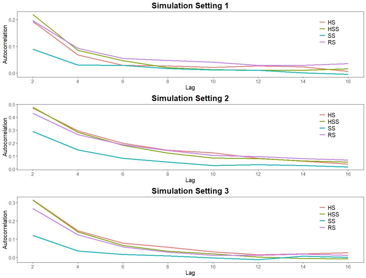
Figure 1: Autocorrelations for SS, HS, HSS, and RS algorithms

While it is true that the SS Gibbs algorithm seems to be marginally better than the others in this particular case, recall that it remains unknown whether the corresponding Markov chain is geometrically ergodic. On the other hand, the HS chain (and the HSS chain - see Subsection 3.2) are both known to be geometrically ergodic. Thus, in order to ensure reliability, we recommend the two “known quantities.”

3 The Hybrid Scan Sandwich Algorithm

In this section, we explain how to add sandwich steps to the HS Gibbs sampler to form the hybrid scan sandwich (HSS) algorithm. There are four subsections. The basic sandwich algorithm of Hobert and Marchev (2008) is described in Subsection 3.1. A generic description of the HSS algorithm is provided in Subsection 3.2. In Subsection 3.3, we illustrate the techniques using the Student’s $t$ example from the Introduction. Finally, in Subsection 3.4, we develop a HSS algorithm for the intractable posterior associated with the mixed model discussed in Section 2.

3.1 The sandwich algorithm

In keeping with the notation of the Introduction, recall that the transition associated with a single iteration of the DA algorithm may be represented as

Building on ideas in Liu and Wu (1999), Meng and van Dyk (1999) and van Dyk and Meng (2001), Hobert and Marchev (2008) introduced an alternative to the DA algorithm that employs an extra move on the $\mathsf{Z}$ space that is “sandwiched” between the two conditional draws. If the extra move is chosen carefully, it can break the correlation between consecutive iterates of the DA algorithm, thereby speeding up the algorithm. Again, using notation from the Introduction, let $f_{Z}$ denote the $z$-marginal of $f(u,z)$, and suppose that $R(z,dz^{\prime})$ is any Markov transition function (Mtf) that is reversible with respect to $f_{Z}$, i.e., $R(z,dz^{\prime})f_{Z}(z)dz=R(z^{\prime},dz)f_{Z}(z^{\prime})dz^{\prime}$. The sandwich algorithm simulates the Markov chain whose Mtd is

$$k_{\text{S}}(u^{\prime}|u)=\int_{\mathsf{Z}}\int_{\mathsf{Z}}f_{U|Z}(u^{\prime}|z^{\prime})R(z,dz^{\prime})f_{Z|U}(z|u)\,dz\;.$$

It’s easy to see that $k_{\text{S}}(u^{\prime}|u)f_{U}(u)$ is symmetric in $(u,u^{\prime})$, so the sandwich Markov chain is reversible with respect to $f_{U}$. Also, the sandwich algorithm reduces to DA if we take $R$ to be the trivial Mtf whose chain never moves from the starting point. To run the sandwich algorithm, we simply run the DA algorithm as usual, except that after each $z$ is drawn, we perform the extra step $z^{\prime}\sim R(z,\cdot)$ before drawing the new $u$. Hence, the sequence of steps in a single iteration of the sandwich algorithm looks like this:

We now explain how a sandwich step can effectively break the correlation between $U$ and $U^{\prime}$ in the context of a toy example.

Suppose the target density is

$$f_{U}(u)=\int_{\mathbb{R}}\frac{1}{\sqrt{8\pi}}e^{-\frac{1}{2}(u-z)^{2}-|z|}\;dz\;.$$

In order to construct a DA algorithm, we require a joint density whose $u$-marginal is the target. Here’s an obvious candidate:

$$f_{U,Z}(u,z)=\frac{1}{\sqrt{8\pi}}e^{-\frac{1}{2}(u-z)^{2}-|z|}\;.$$

Note that $f_{Z}(z)=\frac{1}{2}e^{-|z|}$, so the marginal distribution of $Z$ is standard Laplace (or double exponential). In order to run the DA algorithm, we need the full conditionals. Clearly, $U|Z\sim\mbox{N}(Z,1)$, but the distribution of $Z$ given $U$ is non-standard:

$$f_{Z|U}(z|u)\propto e^{-\frac{1}{2}(u-z)^{2}-|z|}\;.$$

It’s a simple matter to simulate from this density using a rejection sampler with a Laplace candidate. We now construct a sandwich algorithm. Define a Mtf on $\mathbb{R}$ as follows:

$$R(z,dz^{\prime})=r(z^{\prime}|z)dz^{\prime}=e^{-|z^{\prime}|}\big{[}I_{\mathbb{R}_{+}}(z^{\prime})I_{\mathbb{R}_{+}}(z)+I_{\mathbb{R}_{-}}(z^{\prime})I_{\mathbb{R}_{-}}(z)\big{]}dz^{\prime}\;,$$

where $\mathbb{R}_{-}:=(-\infty,0]$. It’s clear that $R(z,dz^{\prime})$ is reversible with respect to $f_{Z}(z)$. Note that the Markov chain defined by $R$ is not irreducible. In fact, the chain remains forever on whichever side of zero it is started. We now provide some intuition about how the extra step breaks the correlation between $U$ and $U^{\prime}$. Imagine for a moment that $r(z^{\prime}|z)$ were just $f_{Z}(z^{\prime})$. Then $U^{\prime}$ would be a perfect draw from $f_{U}$ (independent of $U$), and the Markov chain would simply be an iid sequence from the target distribution. Of course, $r(z^{\prime}|z)$ is not $f_{Z}(z^{\prime})$, but it actually isn’t that far from it. First, $r(z^{\prime}|z)$ depends on $z$ only through its sign. Now, when $z>0$, $r(z^{\prime}|z)$ is nothing but $f_{Z}(z^{\prime})$ truncated to the positive half-line, and when $z\leq 0$, $r(z^{\prime}|z)$ is just $f_{Z}(z^{\prime})$ truncated to the negative half-line. So we can interpret the extra step as follows: Once $Z$ is drawn from $f_{Z|U}(\cdot|u)$, the extra step then draws $Z^{\prime}$ from a truncated version of $f_{Z}$. Intuitively, it seems clear that the correlation between $U$ and $U^{\prime}$ should be quite a bit weaker under the sandwich dynamics, than under the DA dynamics. In order to test this empirically, we ran stationary versions of each chain for one million iterations, and constructed the autocorrelation plot in Figure 2 using the function $V(u)=u^{2}$. Clearly, the autocorrelation of the sandwich Markov chain decays to zero much more rapidly than that of the corresponding DA chain.

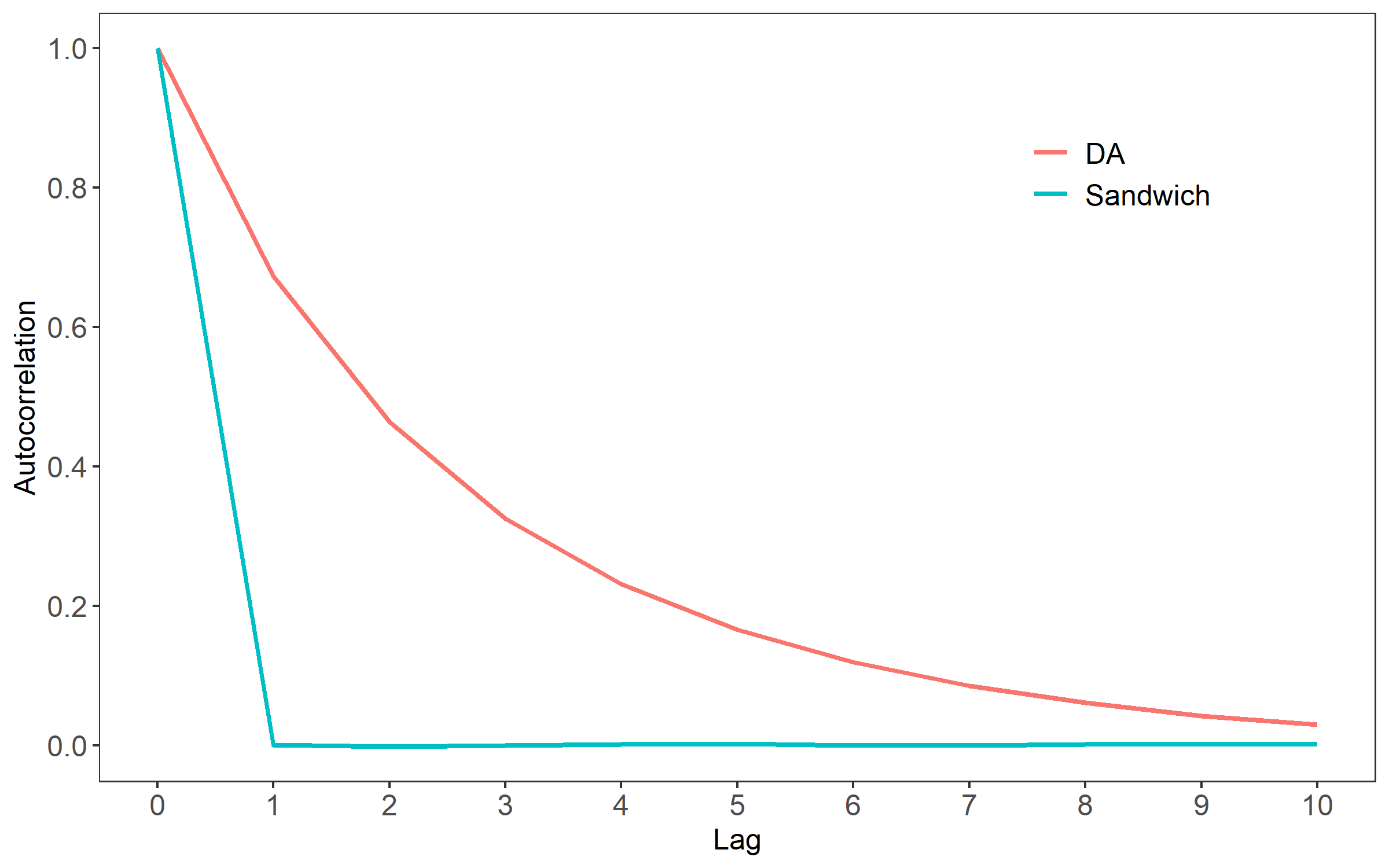
Figure 2: Autocorrelations for the DA and sandwich algorithms

Of course, a sandwich algorithm is a useful alternative to the underlying DA algorithm only if the computational burden of drawing from $R$ is small relative to the improvement it provides. Consider, for example, the Mtf $R(z,dz^{\prime})=r(z^{\prime}|z)dz^{\prime}$ where $r(z^{\prime}|z)=\int_{\mathsf{U}}f_{Z|U}(z^{\prime}|u)f_{U|Z}(u|z)du$. This $R$ leads to a sandwich algorithm that is nothing but two consecutive iterations of the DA algorithm. Thus, whatever is gained by adding the extra step is offset exactly in increased computational effort. Fortunately, it is often possible to find an $R$ that leads to a significant improvement, while adding very little to the overall computational cost. This is typically accomplished by choosing $R(z,dz^{\prime})$ such that, for fixed $z$, the (reducible) chain driven by $R(z,\cdot)$ lives in a low dimensional subspace of $\mathsf{Z}.$ (Note that such an $R$ would typically not have a Mtd with respect to Lebesgue measure on $\mathsf{Z}$, and this is the reason why it is defined via its Mtf, instead of a Mtd.)

There are a couple of simple techniques for constructing sandwich moves (see, e.g., Hobert and Marchev, 2008; Liu and Wu, 1999), and the resulting Mtfs can often be simulated with relatively little computational effort. In such cases, there is nothing to lose by adding the step. In other cases, where simulation of the extra step requires substantial computational effort, one must decide if the trade-off is worthwhile. There are many examples of sandwich algorithms that drastically outperform their DA counterparts in empirical studies, see, e.g., Liu and Wu (1999) and Meng and van Dyk (1999). Moreover, the superiority of the sandwich algorithm has also been established theoretically. Indeed, results in Hobert and Marchev (2008) and Khare and Hobert (2011) show that, under mild regularity conditions, the sandwich algorithm converges at least as fast as the DA algorithm, and is at least as good in the sense of asymptotic variance.

3.2 The HSS algorithm

We now explain how to add up to two different sandwich steps to the HS Gibbs sampler. Recall that the transition mechanism for each iteration of HS Gibbs with selection probability $r$ is given by

For fixed $y\in\mathsf{Y},$ let $R_{1}(z,dz^{\prime};y)$ denote a Mtf on $\mathsf{Z}$ that is reversible with respect to $f_{Z|Y}(z|y),$ so that

$$R_{1}(z,dz^{\prime};y)f_{Z|Y}(z|y)dz=R_{1}(z^{\prime},dz;y)f_{Z|Y}(z^{\prime}|y)dz^{\prime}\;.$$ (5)

Define

$$k_{1}(x^{\prime}|x;y)=\int_{\mathsf{Z}}\int_{\mathsf{Z}}f_{X|Y,Z}(x^{\prime}|y,z^{\prime})R_{1}(z,dz^{\prime};y)f_{Z|X,Y}(z|x,y)\,dz\;.$$

A routine calculation shows that $k_{1}(x^{\prime}|x;y)f_{X|Y}(x|y)$ is symmetric in $(x,x^{\prime})$, so $k_{1}(x^{\prime}|x;y)$ is reversible with respect to $f_{X|Y}(x|y)$. Analogously, for fixed $x\in\mathsf{X}$, define

$$k_{2}(y^{\prime}|y;x)=\int_{\mathsf{Z}}\int_{\mathsf{Z}}f_{Y|X,Z}(y^{\prime}|x,z^{\prime})R_{2}(z,dz^{\prime};x)f_{Z|X,Y}(z|x,y)\,dz\;,$$

where $R_{2}(z,dz^{\prime};x)$ is reversible with respect to $f_{Z|X}(z|x)$.

The HSS algorithm is simply a RS algorithm which, at each iteration, employs either $k_{1}(x^{\prime}|x;y)$ or $k_{2}(y^{\prime}|y;x)$. In particular, fix $r\in(0,1)$, and consider a Markov chain $\{(\tilde{X}_{n},\tilde{Y}_{n})\}_{n=0}^{\infty}$ with state space $\mathsf{X}\times\mathsf{Y}$ that evolves as follows. If the current state is $(\tilde{X}_{n},\tilde{Y}_{n})=(x,y)$, then we simulate the new state, $(\tilde{X}_{n+1},\tilde{Y}_{n+1})$, using the following two-step procedure.

  Iteration $n+1$ of the HSS algorithm:

1. Draw $Z\sim f_{Z|X,Y}(\cdot|x,y)$, call the result $z$, and, independently, draw $W\sim\text{Uniform}(0,1)$.

2. 1. If $W\leq r$, draw $Z^{\prime}\sim R_{1}(z,\cdot;y)$, call the result $z^{\prime}$, draw $X^{*}\sim f_{X|Y,Z}(\cdot|y,z^{\prime})$, and set $(\tilde{X}_{n+1},\tilde{Y}_{n+1})=(X^{*},y)$.

   2. Otherwise if $r<W\leq 1$, draw $Z^{\prime}\sim R_{2}(z,\cdot;x)$, call the result $z^{\prime}$, draw $Y^{*}\sim f_{Y|X,Z}(\cdot|x,z^{\prime})$, and set $(\tilde{X}_{n+1},\tilde{Y}_{n+1})=(x,Y^{*})$.

 

Thus, the HSS algorithm makes the following transition at each iteration.

If we take both $R_{1}$ and $R_{2}$ to be trivial, then the HSS algorithm collapses back into the HS Gibbs sampler. In Appendix A, we develop theoretical results for the HSS algorithm. We begin by showing that the HSS algorithm is reversible, which allows us to prove analogues for the HSS algorithm of the strong theoretical results that have been established for the basic sandwich algorithm. In particular, we prove that the HSS algorithm is always at least as good as HS Gibbs in terms of asymptotic variance, and that the HSS Markov chain converges at least as fast as the HS Gibbs chain as long as the Markov operators associated with $R_{1}$ and $R_{2}$ are both positive. (All of the $R$s employed in this paper, including the trivial $R$, yield positive Markov operators - see Hobert and Marchev (2008).) One important consequence of the convergence rate result is that, when $R_{1}$ and $R_{2}$ are both positive operators, geometric ergodicity of the HS Gibbs Markov chain implies that of the HSS chain.

This is extremely useful in practice because the HS Gibbs algorithm is much simpler than the HSS algorithm, and hence much easier to analyze.

We should point out that Pal et al. (2015) also developed an alternative to SS and RS Gibbs for Bayesian latent data models that is based on the sandwich methodology of Hobert and Marchev (2008). Unfortunately, it is difficult to obtain theoretical results for their algorithm because the corresponding Markov chain is not reversible.

Recall that near the end of the Introduction we considered a generalization in which $U$ is partitioned into three or more pieces, and we wrote the corresponding conditional densities as $f_{X_{j}|X_{-j},Z}$ for $j=1,\dots,s$. It is a simple matter to extend the methodology described above to this more general case. Indeed, for fixed $X_{-j}=x_{-j}$, let $R_{j}(z,dz^{\prime};x_{-j})$ denote a Mtf on $\mathsf{Z}$ that is reversible with respect to $f_{Z|X_{-j}}(z|x_{-j})$. Define

$$k_{j}(x^{\prime}_{j}|x_{j};x_{-j})=\int_{\mathsf{Z}}f_{X_{j}|X_{-j},Z}(x^{\prime}|x_{-j},z^{\prime})R_{j}(z,dz^{\prime};x_{-j})f_{Z|X_{j},X_{-j}}(z|x_{j},x_{-j})\,dz\;.$$

At each step of the generalized version of HSS, we choose among $k_{1},\ldots,k_{s}$ according to positive probabilities $a_{1},\dots,a_{s}$ in the usual way, and apply the chosen $k_{j}$. All of the theoretical results that we establish for the HSS algorithm in Appendix A can be easily extended to this generalization.

3.3 Student’s $t$ example

Consider again the first Student’s $t$ model from the Introduction (with prior $\pi(\mu,\sigma^{2})\propto\sigma^{-2}I_{\mathbb{R}^{+}}(\sigma^{2})$). We now develop a HSS algorithm for this model. Of course, we already know that this model can be handled by the usual DA algorithm, so our HSS algorithm would never be used in practice. However, we believe that it is instructive to demonstrate the construction of a HSS algorithm in a simple context where the details of the model are not themselves overwhelming.

The first step is to identify the distributions of $Z|\mu$ and $Z|\sigma^{2}$. Let $z_{\cdot}=\sum_{i=1}^{m}z_{i}$. It’s easy to show that

$$f_{Z|\mu}(z|\mu) \propto\bigg{(}\sum_{i=1}^{m}z_{i}(w_{i}-\mu)^{2}\bigg{)}^{-\frac{m}{2}}\Bigg{[}\prod_{i=1}^{m}z_{i}\Bigg{]}^{\frac{\nu-1}{2}}\exp\bigg{\{}\!-\frac{z_{\cdot}\nu}{2}\bigg{\}}\prod_{i=1}^{m}I_{\mathbb{R}^{+}}(z_{i})\;.$$

Let $g\in\mathbb{R}_{+}$. It follows from the group theoretic arguments in Hobert and Marchev (2008) that the move $z\mapsto gz$ for $z=(z_{1},\ldots,z_{m})$ is reversible with respect to $f_{Z|\mu}(z|\mu)$ if $g$ is drawn from the density proportional to $f_{Z|\mu}(gz|\mu)g^{m-1}$. (This is a low-dimensional move since, for fixed $z\in\mathbb{R}_{+}^{m}$, the points $gz$ all lie on a ray emanating from the origin and passing through the point $z$.) As a function of $g$, we have

$$f_{Z|\mu}(gz|\mu)g^{m-1} \propto g^{\frac{m\nu}{2}-1}\exp\bigg{\{}\!-\frac{g\nu z_{\cdot}}{2}\bigg{\}}\Bigg{[}\prod_{i=1}^{m}I_{\mathbb{R}^{+}}(z_{i})\Bigg{]}I_{\mathbb{R}^{+}}(g)\;,$$

which is a $\text{Gamma}\big{(}\frac{m\nu}{2},\frac{\nu z_{\cdot}}{2}\big{)}$ density. Now, it’s easy to show that

$$f_{Z|\sigma^{2}}(z|\sigma^{2}) \propto\frac{1}{\sqrt{z_{\cdot}}}\exp\bigg{\{}\!-\frac{z_{\cdot}v(z,w)}{2\sigma^{2}}\bigg{\}}\Bigg{[}\prod_{i=1}^{m}z_{i}\Bigg{]}^{\frac{\nu-1}{2}}\exp\bigg{\{}\!-\frac{z_{\cdot}\nu}{2}\bigg{\}}\prod_{i=1}^{m}I_{\mathbb{R}^{+}}(z_{i})\;,$$

where

$$v(z,w)=\frac{1}{z_{\cdot}}\sum_{i=1}^{m}z_{i}\big{(}w_{i}-\theta(z,w)\big{)}^{2}\;,$$

and $\theta(z,w)=\frac{1}{z_{\cdot}}\sum_{i=1}^{m}z_{i}w_{i}$. Using the same transformation, $z\mapsto gz$, we need to sample $g$ from the density proportional to $f_{Z|\sigma^{2}}(gz|\sigma^{2})g^{m-1}$. A straightforward calculation shows that, as a function of $g$, we have

$$f_{Z|\sigma^{2}}(gz|\sigma^{2})g^{m-1} \propto g^{\frac{m(\nu+1)-3}{2}}\exp\left\{-gz_{.}\bigg{(}\frac{v(z,w)}{2\sigma^{2}}+\frac{\nu}{2}\bigg{)}\right\}\;,$$

which is a $\text{Gamma}\Big{(}\frac{m(\nu+1)-1}{2},z_{.}\big{(}\frac{v(z,w)}{2\sigma^{2}}+\frac{\nu}{2}\big{)}\Big{)}$ density.

Fix a selection probability $r\in(0,1)$ and consider the Markov chain $\{(\tilde{\mu}_{n},\tilde{\sigma}^{2}_{n})\}_{n=0}^{\infty}$ with state space $\mathbb{R}\times\mathbb{R}_{+}$. The HSS algorithm proceeds as follows. If the current state is $(\tilde{\mu}_{n},\tilde{\sigma}^{2}_{n})=(\mu,\sigma^{2})$, then we simulate the next state, $(\tilde{\mu}_{n+1},\tilde{\sigma}^{2}_{n+1}),$ by performing the following two steps:

  Iteration $n+1$ of the HSS algorithm for the Student’s $t$ example:

1. Draw $Z_{1},\ldots,Z_{m}$ independently, with

   $$Z_{i}\sim\text{Gamma}\left(\frac{\nu+1}{2},\frac{1}{2}\left(\frac{(w_{i}-\mu)^{2}}{\sigma^{2}}+\nu\right)\right)\;,$$

   call the observed values $z=(z_{1},\ldots,z_{m}),$ and, independently, draw $W\sim\text{Uniform}(0,1).$

2. 1. If $W\leq r,$ draw

      $$g\sim\text{Gamma}\bigg{(}\frac{m\nu}{2},\frac{\nu z_{\cdot}}{2}\bigg{)}\,,$$

      then draw

      $$\sigma^{*2}\sim\text{IG}\bigg{(}\frac{m}{2},\frac{1}{2}\sum_{i=1}^{m}gz_{i}(y_{i}-\mu)^{2}\bigg{)},$$

      and set $(\tilde{\mu}_{n+1},\tilde{\sigma}^{2}_{n+1})=(\mu,\sigma^{*2}).$

   2. Otherwise if $r<W\leq 1,$ draw

      $$g\sim\text{Gamma}\bigg{(}\frac{m(\nu+1)-1}{2},z_{.}\Big{(}\frac{v(z,w)}{2\sigma^{2}}+\frac{\nu}{2}\Big{)}\bigg{)}\;,$$

      and then draw

      $$\mu^{*}\sim\text{N}\left(\theta(z,w),\frac{\sigma^{2}}{gz_{.}}\right),$$

      and set $(\tilde{\mu}_{n+1},\tilde{\sigma}^{2}_{n+1})=(\mu^{*},\sigma^{2})$.

 

In terms of computation, the difference between running one iteration of this HSS algorithm versus one iteration of the HS Gibbs sampler upon which it is based is a single draw from the gamma distribution. Thus, if $m$ is even moderately large, this extra draw would add relatively little to the overall computational effort of the HS Gibbs algorithm.

3.4 General linear mixed model example

Abrahamsen and Hobert (2019) introduced and analyzed the HS Gibbs sampler described in Section 2, but they did not consider adding sandwich steps to their algorithm. In this subsection, we develop a HSS algorithm with a single sandwich step based on the conditional density $\pi(\tau|\theta,y)$. (It is much more difficult to construct a sandwich step based on $\pi(\tau|\lambda,y)$.) A routine calculation shows that

$$\pi(\tau|\theta,y)\propto\left(\frac{\lVert{y-W\theta}\rVert^{2}}{2}+\frac{\beta^{T}D_{\tau}^{-1}\beta}{2}+b_{0}\right)^{-\left(\frac{N}{2}+\frac{p}{2}+a_{0}\right)}\prod_{j=1}^{p}\tau_{j}^{c-\frac{3}{2}}e^{-d\tau_{j}}I_{\mathbb{R}_{+}}(\tau_{j})\,.$$

As in the previous subsection, the move $\tau\mapsto g\tau$ is reversible with respect to $\pi(\tau|\theta,y)$ if $g$ is drawn from the density proportional to $\pi(g\tau|\theta,y)g^{p-1}I_{\mathbb{R}_{+}}(g)$. Now, as a function of $g$,

$$\pi(g\tau|\theta,y)\propto\left(\frac{\lVert{y-W\theta}\rVert^{2}}{2}+\frac{g^{-1}\beta^{T}D_{\tau}^{-1}\beta}{2}+b_{0}\right)^{-\left(\frac{N}{2}+\frac{p}{2}+a_{0}\right)}g^{p(c-\frac{3}{2})}e^{-g\left(d\sum_{j=1}^{p}\tau_{j}\right)}\prod_{j=1}^{p}I_{\mathbb{R}_{+}}(\tau_{j})\;,$$

so the density from which $g$ must be drawn is given by

$$h(g;\tau,\theta,y)\propto\frac{g^{\frac{N}{2}+cp+a_{0}-1-s}}{\left(\frac{\beta^{T}D_{\tau}^{-1}\beta}{2}+g\left(\frac{\lVert{y-W\theta}\rVert^{2}}{2}+b_{0}\right)\right)^{\frac{N}{2}+\frac{p}{2}+a_{0}}}\;\left[g^{s}e^{-g\left(d\sum_{j=1}^{p}\tau_{j}\right)}\right]I_{\mathbb{R}_{+}}(g)\;,$$

where $s>0$ is a free parameter. So,

$$h(g;\tau,\theta,y)\propto\frac{g^{\frac{N}{2}+cp+a_{0}-1-s}}{(1+Cg)^{\frac{N}{2}+\frac{p}{2}+a_{0}}}\;\left[g^{s}e^{-g\left(d\sum_{j=1}^{p}\tau_{j}\right)}\right]I_{\mathbb{R}_{+}}(g)\;,$$ (6)

where

$$C=\frac{\lVert{y-W\theta}\rVert^{2}+2b_{0}}{\beta^{T}D_{\tau}^{-1}\beta}\;.$$

If we choose $s\in\Big{(}\max\Big{\{}0,\;p\big{(}c-\frac{1}{2}\big{)}\Big{\}},\frac{N}{2}+cp+a_{0}\Big{)}$, then two things happen: (1) the first term on the right-hand side of  (6) is proportional to a scaled $F$ density, and (2) the second term is bounded. In fact, the second term achieves its maximum at $\hat{g}=s\big{(}d\sum_{j=1}^{p}\tau_{j}\big{)}^{-1}$. Thus, we can use a simple accept/reject algorithm with an $F$ candidate to draw from $h.$ In particular, let $\nu_{1}=N+2cp+2a_{0}-2s$ and $\nu_{2}=p(1-2c)+2s.$ Here’s the algorithm.

  Accept/Reject algorithm for $h$:

1. Draw $V^{*}\sim F(\nu_{1},\nu_{2}),$ set $V=(V^{*}\nu_{1})/(C\nu_{2}),$ and independently draw $U\sim\text{Uniform}(0,1).$

2. If

   $$U\leq\left(\frac{dV\sum_{j=1}^{p}\tau_{j}}{s}\right)^{s}\;e^{s-dV\sum_{j=1}^{p}\tau_{j}},$$

   then accept $V$ as a draw from  (6), otherwise return to 1.

 

If $r\in(0,1)$ is the selection probability, then our HSS algorithm proceeds as follows. Let the current state of the chain be $(\theta_{n},\lambda_{n})=(\theta,\lambda)$. First, draw $\tau\sim\pi(\tau|\theta,\lambda,y)$, and then flip an $r$-coin. If the coin comes up heads, we move to $(\theta_{n+1},\lambda_{n+1})=(\theta,\lambda^{*})$ by first drawing $g\sim h(\cdot;\tau,\theta,y)$ and then drawing $\lambda^{*}\sim\pi(\lambda|\theta,g\tau,y)$. If the coin comes up tails, we move to $(\theta_{n+1},\lambda_{n+1})=(\theta^{*},\lambda)$ by drawing $\theta^{*}\sim\pi(\theta|\lambda,\tau,y)$. Another, perhaps simpler, way to describe the HSS algorithm is via a simple modification of the HS Gibbs algorithm described in Section 2. Step 1 remains exactly the same. In step 2, if $r<W\leq 1$, then, again, nothing changes. However, if $W\leq r$, then, instead of using $\tau$ from step 1, we draw $g\sim h(\cdot;\tau,\theta,y)$, and use $g\tau$ in place of $\tau$.

It follows from Proposition 2 in Appendix A that, whenever the HS Gibbs sampler of Section 2 is geometrically ergodic, so is our HSS algorithm. Recall that some empirical results for this HSS algorithm are depicted alongside the results for the HS, SS, and RS Gibbs samplers in Figure 1 of Section 2. In that example, the rejection sampler is quite efficient, with an acceptance probability of more than 70% in each of the three simulations settings considered. The per iteration computational cost of HS Gibbs obviously grows with $p$ while the extra cost associated with rejection sampling is basically constant in $p$. As a result, in the second and third simulation settings, the HSS algorithm was only about 2% slower than HS Gibbs, while in the first setting, the HSS algorithm is substantially slower than HS Gibbs. Note that the performance of the rejection sampler is a function of $C$ and $\sum_{j=1}^{p}\tau_{j}$. For these simulations, we developed a table in a preliminary offline investigation to decide the appropriate value of the free parameter $s$ for a given $\big{(}C,\sum_{j=1}^{p}\tau_{j}\big{)}$ pair.

4 Bayesian Linear Regression with Scale Mixtures of Normal Errors

In this section, we provide another example of a Bayesian model that leads to a highly intractable posterior distribution that lends itself to the HS Gibbs sampler. Let $Y_{1},\ldots,Y_{m}$ be independent random variables from the linear regression model

$$Y_{i}=x_{i}^{T}\beta+\sigma\epsilon_{i}\;,$$ (7)

where $x_{i}$ is a $p\times 1$ vector of known covariates associated with $Y_{i}$, $\beta$ is a $p\times 1$ vector of unknown regression coefficients, $\sigma\in(0,\infty)$ is an unknown scale parameter, and $\epsilon_{1},\ldots,\epsilon_{m}$ are iid errors. The standard assumption that the errors are Gaussian is often inappropriate, e.g., when the data contain outliers. Various heavy-tailed alternatives can be constructed as scale mixtures of the Gaussian density. Consider an error density of the form

$$f_{H}(\epsilon)=\int_{0}^{\infty}\frac{\sqrt{z}}{\sqrt{2\pi}}\exp\left\{-\frac{z}{2}\epsilon^{2}\right\}\,dH(z)\;,$$ (8)

where $H$ is the distribution function of some non-negative random variable. By varying the mixing distribution $H$, many symmetric and unimodal distributions can be constructed. Thus, datasets with various types of tail behavior (particularly with heavier tails than the normal) are often modeled by choosing a distribution from this class. In this section, we consider a Bayesian analysis of the linear regression model  (7) when the errors $\epsilon_{1},\ldots,\epsilon_{m}$ are iid random variables with the general scale mixture of normals density $f_{H}$ given in  (8). There are several different prior distributions available that lead to conditional distributions with standard forms. Hobert et al. (2018) consider a standard improper prior and show that a DA algorithm is available. A DA algorithm is also available in the case where we specify a proper conditionally conjugate prior on $(\beta,\sigma^{2})$ by setting $\beta|\sigma^{2}\sim\mbox{N}_{p}(\mu,\sigma^{2}\Sigma)$ and $\sigma^{2}\sim\mbox{IG}(\alpha,\gamma)$. Throughout this section, we will instead consider the proper prior which takes $\beta$ and $\sigma^{2}$ to be a priori independent with $\beta\sim\mbox{N}_{p}(\mu,\Sigma)$ and $\sigma^{2}\sim\mbox{IG}(\alpha,\gamma)$. This slight change to the prior makes the DA algorithm difficult to implement, but the HS Gibbs sampler is a viable alternative. We now provide the details.

Let $y=(y_{1},\ldots,y_{m})$ denote the observed data. Let $X$ denote the $m\times p$ matrix whose $i$th row is $x_{i}^{T}$. We assume throughout that $m\geq\max\{2,p\}$. We also assume that $H$ has a density, $h$, with respect to Lebesgue measure on $\mathbb{R}_{+}$. Letting $p_{H}(y|\beta,\sigma^{2})$ denote the joint density of the data from the linear regression model, the posterior density is given by

$$\pi(\beta,\sigma^{2}|y) \propto p_{H}(y|\beta,\sigma^{2})\pi(\beta,\sigma^{2})$$

$$\propto\Bigg{[}\prod_{i=1}^{m}\frac{1}{\sigma}f_{H}\left(\frac{y_{i}-x_{i}^{T}\beta}{\sigma}\right)\Bigg{]}\pi(\beta,\sigma^{2})$$

$$\propto\Bigg{[}\prod_{i=1}^{m}\int_{\mathbb{R}_{+}}\frac{\sqrt{z_{i}}}{\sqrt{2\pi\sigma^{2}}}\exp\left\{-\frac{z_{i}}{2}\frac{(y_{i}-x_{i}^{T}\beta)^{2}}{\sigma^{2}}\right\}h(z_{i})\,dz_{i}\Bigg{]}$$

$$\hskip 22.76219pt\times(\sigma^{2})^{-\alpha-1}\exp\left\{-\frac{\gamma}{\sigma^{2}}\right\}\exp\left\{-\frac{(\beta-\mu)^{T}\Sigma^{-1}(\beta-\mu)}{2}\right\}I_{\mathbb{R}^{+}}(\sigma^{2})\;.$$

Define the complete data posterior density as

$$\pi(\beta,\sigma^{2},z|y) =\prod_{i=1}^{m}\frac{\sqrt{z_{i}}}{\sqrt{2\pi\sigma^{2}}}\exp\left\{-\frac{z_{i}}{2}\frac{(y_{i}-x_{i}^{T}\beta)^{2}}{\sigma^{2}}\right\}h(z_{i})$$

$$\times(\sigma^{2})^{-\alpha-1}\exp\left\{-\frac{\gamma}{\sigma^{2}}\right\}\exp\left\{-\frac{(\beta-\mu)^{T}\Sigma^{-1}(\beta-\mu)}{2}\right\}I_{\mathbb{R}^{+}}(\sigma^{2})\;,$$

and note that $\int_{\mathbb{R}_{+}^{m}}\pi(\beta,\sigma^{2},z|y)\,dz=\pi(\beta,\sigma^{2}|y)$, so that $z=(z_{1},\ldots,z_{m})$ constitutes latent data. We now state the conditional densities needed for the HS Gibbs sampler. First, conditional on $(\beta,\sigma^{2},y)$, $z_{1},\ldots,z_{m}$ are independent, and the conditional density of $z_{i}$ given $(\beta,\sigma^{2},y_{i})$ is given by

$$\pi(z_{i}|\beta,\sigma^{2},y_{i})\propto z_{i}^{\frac{1}{2}}\exp\left\{-\frac{z_{i}}{2}\frac{(y_{i}-x_{i}^{T}\beta)^{2}}{\sigma^{2}}\right\}h(z_{i})\;.$$ (9)

In some cases, this density turns out to be standard. For example, when $h$ is a gamma density, then so is $\pi(z_{i}|\beta,\sigma^{2},y_{i})$, and when $h$ is inverted gamma, then $\pi(z_{i}|\beta,\sigma^{2},y_{i})$ is generalized inverse Gaussian. Even when it’s not a standard density, as long as one can make draws from $h$, then $h$ can be used as the candidate in a simple rejection sampler.

Next, let $Q$ be an $m\times m$ diagonal matrix whose $i$th diagonal element is $z_{i}^{-1}$. We have

$$\sigma^{2}\;|\;\beta,z,y\sim\text{IG}\left(\frac{m}{2}+\alpha,\frac{(y-X\beta)^{T}Q^{-1}(y-X\beta)+2\gamma}{2}\right)\;.$$

Finally, $\beta\;|\;\sigma^{2},z,y\sim\mbox{N}_{p}\left(\mu^{\prime},\sigma^{2}\Sigma^{\prime}\right)$, where

$$\mu^{\prime}=\left(X^{T}Q^{-1}X+\sigma^{2}\Sigma^{-1}\right)^{-1}\left(X^{T}Q^{-1}y+\sigma^{2}\Sigma^{-1}\mu\right)\hskip 14.22636pt\mbox{and}\hskip 14.22636pt\Sigma^{\prime}=\left(X^{T}Q^{-1}X+\sigma^{2}\Sigma^{-1}\right)^{-1}\;.$$

The HS Gibbs sampler is based on the Markov chain $\Phi=\{(\beta_{n},\sigma_{n}^{2})\}_{n=0}^{\infty}$ with state space $\mathsf{X}=\mathbb{R}^{p}\times\mathbb{R}_{+}$ and selection probability $r\in(0,1).$ The dynamics of $\Phi$ are defined by the following two step procedure for moving from $(\beta_{n},\sigma_{n}^{2})=(\beta,\sigma^{2})$ to $(\beta_{n+1},\sigma_{n+1}^{2}).$

  Iteration $n+1$ of the hybrid scan Gibbs sampler:

1. Draw $Z_{1},\ldots,Z_{m}$ independently with

   $$Z_{i}\sim\text{the density proportional to}\;z_{i}^{\frac{1}{2}}\exp\left\{-\frac{z_{i}}{2}\frac{(y_{i}-x_{i}^{T}\beta)^{2}}{\sigma^{2}}\right\}h(z_{i})\;,$$

   call the observed values $z=(z_{1},\ldots,z_{m}),$ and, independently, draw $W\sim\text{Uniform}(0,1).$

2. 1. If $W\leq r,$ draw

      $$\sigma^{*2}\sim\text{IG}\left(\frac{m}{2}+\alpha,\frac{(y-X\beta)^{T}Q^{-1}(y-X\beta)+2\gamma}{2}\right),$$

      and set $(\beta_{n+1},\sigma_{n+1}^{2})=(\beta,\sigma^{*2}).$

   2. Otherwise if $r<W\leq 1,$ draw

      $$\beta^{*}\sim\mbox{N}_{p}\left(\mu^{\prime},\sigma^{2}\Sigma^{\prime}\right),$$

      and set $(\beta_{n+1},\sigma_{n+1}^{2})=(\beta^{*},\sigma^{2}).$

 

We now provide convergence rate results for this HS algorithm and the corresponding SS Gibbs sampler. Let $\hat{\Phi}=\{(\hat{\beta}_{n},\hat{\sigma}_{n}^{2})\}_{n=0}^{\infty}$ denote the Markov chain defined by the following Mtd:

$$k_{\text{G}}(\beta,\sigma^{2}|\hat{\beta},\hat{\sigma}^{2})=\int_{\mathbb{R}_{+}^{n}}\pi(\beta|\sigma^{2},z,y)\pi(\sigma^{2}|\hat{\beta},z,y)\pi(z|\hat{\beta},\hat{\sigma}^{2},y)\,dz\;.$$

Of course, this is just the Markov chain that one is left with when one runs the three-block SS Gibbs sampler and ignores the latent data. It is well known that this chain has exactly the same convergence rate as the SS Gibbs chain. The following result, which is proven in Appendix B, provides sufficient conditions for each of these algorithms to be geometrically ergodic.

Theorem 2.

The following results hold for any mixing density $h.$

1. Suppose there exist constants $0\leq\psi_{1}<1$ and $L_{1}\in\mathbb{R}$ which do not depend on $\beta$ or $\sigma^{2}$ such that

   $$\frac{\sum_{i=1}^{m}E[z_{i}|\beta,\sigma^{2},y](y_{i}-x_{i}^{T}\beta)^{2}}{m+2\alpha-2}\leq\psi_{1}\left[\sum_{i=1}^{m}(y_{i}-x_{i}^{T}\beta)^{2}+\beta^{T}\Sigma^{-1}\beta+\sigma^{2}+\frac{1}{\sigma^{2}}\right]+L_{1}\;$$ (10)

   for every $\beta\in\mathbb{R}^{p},\sigma^{2}\in\mathbb{R}_{+}$. Then $\hat{\Phi}$ is geometrically ergodic.

2. Suppose there exist constants $\psi_{2}\in\mathbb{R}_{+}$, $0\leq\psi_{3}<1$, and $L_{2}\in\mathbb{R}$ which do not depend on $\beta$ or $\sigma^{2}$ such that

   $$\frac{\sum_{i=1}^{m}E[z_{i}|\beta,\sigma^{2},y](y_{i}-x_{i}^{T}\beta)^{2}}{m+2\alpha-2}\leq\psi_{2}\Bigg{[}\sum_{i=1}^{m}(y_{i}-x_{i}^{T}\beta)^{2}+\,\beta^{T}\Sigma^{-1}\beta\Bigg{]}+\psi_{3}\left(\sigma^{2}+\frac{1}{\sigma^{2}}\right)+L_{2}\;$$ (11)

   for every $\beta\in\mathbb{R}^{p},\sigma^{2}\in\mathbb{R}_{+}$. Then $\Phi$ is geometrically ergodic for all $r\in(0,1)$.

Remark 1.

Note that if (10) holds, then (11) holds with $\psi_{2}=\psi_{3}=\psi_{1}$, and $L_{2}=L_{1}$. So the sufficient condition for geometric ergodicity of the HS Gibbs algorithm is weaker than the corresponding sufficient condition for the SS Gibbs sampler. Of course, we are dealing with sufficient conditions here, so by no means does Theorem 2 imply that HS Gibbs algorithm is geometrically ergodic more often than the SS Gibbs sampler. On the other hand, in a given situation, if it is known that the HS algorithm is geometrically ergodic, and it is unknown whether or not the same is true of the SS Gibbs sampler, then one should probably use the HS algorithm.

In order to actually apply Theorem 2, we must specify $h$ so that we can calculate (or at least bound) $E[z_{i}|\beta,\sigma^{2},y]$. For example, suppose that $h$ is a $\text{Gamma}(\frac{\nu}{2},\frac{\nu}{2})$ density, which leads to a Student’s $t$ distribution with $\nu$ degrees of freedom for the regression errors. In this case, $z_{i}|(\beta,\sigma^{2},y)$ is

$$\mbox{Gamma}\bigg{(}\frac{\nu+1}{2},\frac{(y_{i}-x_{i}^{T}\beta)^{2}+\nu\sigma^{2}}{2\sigma^{2}}\bigg{)}\;,$$

and

$$E[z_{i}|\beta,\sigma^{2},y]=\frac{\sigma^{2}(\nu+1)}{(y_{i}-x_{i}^{T}\beta)^{2}+\nu\sigma^{2}}\;.$$

It follows that (11) is satisfied since

$$\frac{\sum_{i=1}^{m}E[z_{i}|\beta,\sigma^{2},y](y_{i}-x_{i}^{T}\beta)^{2}}{m+2\alpha-2} =\frac{1}{m+2\alpha-2}\sum_{i=1}^{m}\frac{\sigma^{2}(\nu+1)(y_{i}-x_{i}^{T}\beta)^{2}}{(y_{i}-x_{i}^{T}\beta)^{2}+\nu\sigma^{2}}$$

$$\leq\frac{\nu+1}{\nu(m+2\alpha-2)}\sum_{i=1}^{m}(y_{i}-x_{i}^{T}\beta)^{2}\;.$$ (12)

Thus, Theorem 2 implies that the HS Markov chain is geometrically ergodic (without any additional assumptions).

Unfortunately, this argument doesn’t work for the SS Gibbs sampler. Indeed, (4) doesn’t establish that (10) is satisfied unless we make the additional assumption that that $\nu>1/(m+2\alpha-3)$. However, another upper bound on the left-hand side of (4) is as follows:

$$\frac{\sum_{i=1}^{m}E[z_{i}|\beta,\sigma^{2},y](y_{i}-x_{i}^{T}\beta)^{2}}{m+2\alpha-2}\leq\frac{m(\nu+1)}{m+2\alpha-2}\sigma^{2}\;.$$ (13)

Now, (13) will establish (10) if $\nu<(2\alpha-2)/m$. So Theorem 2 implies that the SS Gibbs chain is geometrically ergodic if either $\nu>1/(m+2\alpha-3)$ or $\nu<(2\alpha-2)/m$. Of course, if $1/(m+2\alpha-3)<(2\alpha-2)/m$, then at least one of these two inequalities must hold. However, when $\alpha$ is small, this is not the case.

Consider a second example where $h$ is taken to be an $\text{IG}(\alpha,1)$ density. Under this mixing density, the regression errors have a generalized hyperbolic distribution, which has tails that are heavier than Gaussian, but lighter than Student’s $t$ (see, e.g., Jung and Hobert, 2014). In this case, $z_{i}|(\beta,\sigma^{2},y)$ is

$$\mbox{GIG}\bigg{(}\frac{1}{2}-\alpha,\frac{(y_{i}-x_{i}^{T}\beta)^{2}}{\sigma^{2}},2\bigg{)}\;,$$

and

$$E[z_{i}|\beta,\sigma^{2},y]=\frac{\sqrt{2\sigma^{2}}}{\sqrt{(y_{i}-x_{i}^{T}\beta)^{2}}}\frac{\mbox{K}_{-\alpha+3/2}\Big{(}\sqrt{\frac{2(y_{i}-x_{i}^{T}\beta)^{2}}{\sigma^{2}}}\Big{)}}{\mbox{K}_{-\alpha+1/2}\Big{(}\sqrt{\frac{2(y_{i}-x_{i}^{T}\beta)^{2}}{\sigma^{2}}}\Big{)}}\;.$$

Jung (2015, p. 62) shows that

$$\frac{\mbox{K}_{-\alpha+3/2}\Big{(}\sqrt{\frac{2(y_{i}-x_{i}^{T}\beta)^{2}}{\sigma^{2}}}\Big{)}}{\mbox{K}_{-\alpha+1/2}\Big{(}\sqrt{\frac{2(y_{i}-x_{i}^{T}\beta)^{2}}{\sigma^{2}}}\Big{)}}\leq 1+\frac{\sqrt{\sigma^{2}}}{\sqrt{2(y_{i}-x_{i}^{T}\beta)^{2}}}\;.$$

Hence, letting $C>0$ be an arbitrary positive constant, we have

$$\frac{\sum_{i=1}^{m}E[z_{i}|\beta,\sigma^{2},y](y_{i}-x_{i}^{T}\beta)^{2}}{m+2\alpha-2} \leq\frac{1}{m+2\alpha-2}\sum_{i=1}^{m}\bigg{[}\frac{\sqrt{2\sigma^{2}}}{C}\sqrt{C(y_{i}-x_{i}^{T}\beta)^{2}}+\sigma^{2}\bigg{]}$$

$$\leq\frac{1}{m+2\alpha-2}\sum_{i=1}^{m}\bigg{[}\frac{C(y_{i}-x_{i}^{T}\beta)^{2}}{2}+\frac{\sigma^{2}}{C}+\sigma^{2}\bigg{]}$$

$$=\frac{C}{2(m+2\alpha-2)}\sum_{i=1}^{m}(y_{i}-x_{i}^{T}\beta)^{2}+\frac{m(C+1)}{C(m+2\alpha-2)}\sigma^{2}\;.$$ (14)

If $\alpha>1$, then we can find $C>0$ such that $\frac{m(C+1)}{C(m+2\alpha-2)}<1$. Therefore, Theorem 2 implies that the HS Gibbs chain is geometrically ergodic whenever $\alpha>1$.

Now, if we can find a single value of $C>0$ such that $m(C+1)<C(m+2\alpha-2)$ and $C<2(m+2\alpha-2)$, then (4) will imply that (10) holds. The existence of such a $C$ is equivalent to $\alpha$ and $m$ satisfying the following inequality

$$8\alpha^{2}+\alpha(4m-16)+8-5m>0\;.$$

Thus, Theorem 2 implies that the SS Gibbs chain is geometrically ergodic if $\alpha>\big{(}4-m+\sqrt{m(m+2)}\big{)}/4$. This inequality holds for all $\alpha\geq\frac{5}{4}$, regardless of the value of $m$, and it does hold for smaller values of $\alpha$ when $m$ is fixed. For example, if $m=2$, then we only need $\alpha>(1+\sqrt{2})/2\approx 1.21$.

Once $h$ is specified, HSS algorithms can be created by adding sandwich steps to the HS Gibbs sampler. Backlund (2020) develops a HSS algorithm with two sandwich steps for the case where $h$ is a $\text{Gamma}(\frac{\nu}{2},\frac{\nu}{2})$ density.

5 Discussion

We have introduced generic forms of the hybrid scan Gibbs sampler and the hybrid scan sandwich algorithm, and we have shown that, under weak regularity conditions, the latter is theoretically better than the former. Moreover, we have developed and studied specific versions of these algorithms in the context of two different realistic Bayesian hierarchical models. It is clear that the hybrid scan algorithms are quite flexible, and can be used in conjunction with a variety of practical Bayesian models. As another example, consider a generalization of the model in (7) in which the error density has both heavy tails and skewness. da Silva Ferreira et al. (2011) define a skew scale mixture of normal densities, $f_{H,\lambda}(\epsilon)$, by

$$f_{H,\lambda}(\epsilon)=2f_{H}(\epsilon)\Phi(\lambda\epsilon)\;,$$ (15)

where $f_{H}(\epsilon)$ is the scale mixture of normal densities defined at (8), $\Phi(\cdot)$ is the standard normal cumulative distribution function, and $\lambda\in\mathbb{R}$ is a fixed parameter that controls the skewness. Combining the associated likelihood with the same conjugate normal/inverse-gamma prior employed in Section 4 gives rise to a posterior distribution that is even more unwieldy than the one studied in Section 4. However, Jung (2015) shows that there exist two sets of latent variables, $z=(z_{1},\ldots,z_{m})$ and $t=(t_{1},\ldots,t_{m})$, conditionally independent of one another given $(\beta,\sigma^{2},y)$, that give rise to a complete data posterior with the following conditionals. Conditional on $(\beta,\sigma^{2},y)$, $z_{1},\ldots,z_{m}$ are independent, and the density of $z_{i}$ given $(\beta,\sigma^{2},y)$ is the same as (9). Also, conditional on $(\beta,\sigma^{2},y)$, $t_{1},\ldots,t_{m}$ are independent, and the density of $t_{i}$ given $(\beta,\sigma^{2},y)$ is truncated normal. Finally, $\sigma^{2}$ given $(\beta,z,t,y)$ is inverse-gamma, and $\beta$ given $(\sigma^{2},z,t,y)$ is multivariate normal. Unfortunately, the distribution of $\sigma^{2}$ given $(z,t,y)$ is not available in closed form, so that the DA algorithm is not straightforward to apply. Each iteration of the HS Gibbs algorithm proceeds, as usual, by updating (all of) the latent data, and updating either $\beta$ or $\sigma^{2}$, depending on the outcome of the flip of an $r$-coin.

Lastly, we reiterate that, as far as theoretical convergence rates go, it is now generally accepted that one should, if possible, use a Monte Carlo Markov chain that converges at a geometric rate, or at least a rate fast enough to ensure that the corresponding MCMC estimators are asymptotically normal (see, e.g., Roberts and Rosenthal, 1998). Hence, even if an alternative MCMC algorithm (such as SS or RS Gibbs) appears marginally better than a geometrically ergodic HS Gibbs sampler according to empirical measures, that algorithm should not be favored over the HS Gibbs algorithm unless it is known that the alternative has an acceptably fast convergence rate. At present, it appears that the convergence rates of alternative MCMC algorithms for the family of posteriors considered in Section 2 (and, to some extent, those considered in Section 4) are not known. In situations such as these, we recommend HS Gibbs for practical use and remind the reader that it is no more difficult to implement than its SS or RS counterparts.

Acknowledgment. The second and fourth authors were supported by NSF Grant DMS-15-11945.

Appendices

Appendix A Theory for the HSS Algorithm

We begin with some requisite background material on Markov operators. In keeping with the notation in the Introduction, the target density, $f_{X,Y}(x,y),$ can be used to define an inner product

$$\langle g_{1},g_{2}\rangle_{L^{2}_{0}}=\int_{\mathsf{X}}\int_{\mathsf{Y}}g_{1}(x,y)g_{2}(x,y)f_{X,Y}(x,y)\,dy\,dx\;,$$

and norm $\lVert{g}\rVert=\sqrt{\langle g,g\rangle}$ on the Hilbert space

$$L^{2}_{0}=\left\{g:\mathsf{X}\times\mathsf{Y}\to\mathbb{R}:\int_{\mathsf{X}}\int_{\mathsf{Y}}g^{2}(x,y)f_{X,Y}(x,y)\,dy\,dx<\infty\;\text{and}\;\int_{\mathsf{X}}\int_{\mathsf{Y}}g(x,y)f_{X,Y}(x,y)\,dy\,dx=0\right\}\;.$$

To keep things simple, we assume throughout that $f_{X,Y}(x,y)$ is a density with respect to Lebesgue measure, but we note that the results actually hold much more generally - see, e.g., the set-up in Khare and Hobert (2011). The Mtd $k_{1}$ corresponds to a Markov operator $K_{1}:L^{2}_{0}\to L^{2}_{0}$ that takes $g\in L^{2}_{0}$ into

$$(K_{1}g)(x,y)=\int_{\mathsf{X}}g(x^{\prime},y)k_{1}(x^{\prime}|x;y)\,dx^{\prime}\;.$$

Now, if we define $K_{2}$ using $k_{2}$ in an analogous way, then it is clear that the Markov operator associated with the HSS algorithm, $K_{\text{HSS}}:L^{2}_{0}\to L^{2}_{0},$ is given by $K_{\text{HSS}}=rK_{1}+(1-r)K_{2}$, where $r\in(0,1)$ is the selection probability. Here is our first result.

Proposition 1.

The Markov chain underlying the HSS algorithm is reversible.

Proof.

It suffices to show that $K_{\text{HSS}}$ is a self-adjoint operator. We start by showing that $K_{1}$ is self-adjoint. First, it’s easy to see that $f_{X,Y}(x,y)k_{1}(x^{\prime}|x;y)=f_{X,Y}(x^{\prime},y)k_{1}(x|x^{\prime};y).$ It follows that

$$f_{X,Y}(x,y)(K_{1}g)(x,y) =f_{X,Y}(x,y)\int_{\mathsf{X}}g(x^{\prime},y)k_{1}(x^{\prime}|x;y)\,dx^{\prime}$$

$$=\int_{\mathsf{X}}g(x^{\prime},y)f_{X,Y}(x,y)k_{1}(x^{\prime}|x;y)\,dx^{\prime}$$

$$=\int_{\mathsf{X}}g(x^{\prime},y)f_{X,Y}(x^{\prime},y)k_{1}(x|x^{\prime};y)\,dx^{\prime}$$

Thus,

$$\langle K_{1}g,h\rangle_{L^{2}_{0}} =\int_{\mathsf{X}}\int_{\mathsf{Y}}(K_{1}g)(x,y)h(x,y)f_{X,Y}(x,y)\,dy\,dx$$

$$=\int_{\mathsf{X}}\int_{\mathsf{Y}}h(x,y)\left[\int_{\mathsf{X}}g(x^{\prime},y)f_{X,Y}(x^{\prime},y)k_{1}(x|x^{\prime};y)\,dx^{\prime}\right]\,dy\,dx$$

$$=\int_{\mathsf{X}}\int_{\mathsf{Y}}\left[\int_{\mathsf{X}}h(x,y)k_{1}(x|x^{\prime};y)\,dx\right]g(x^{\prime},y)f_{X,Y}(x^{\prime},y)\,dy\,dx^{\prime}$$

$$=\langle g,K_{1}h\rangle_{L^{2}_{0}}\;,$$

where the third equality follows from Fubini’s theorem. Now an analogous argument shows that $K_{2}$ is self-adjoint, and it follows immediately that $rK_{1}+(1-r)K_{2}$ is also self-adjoint. ∎

We now look more closely at the two criteria for comparing MCMC algorithms that were mentioned in the Introduction: rate of convergence and asymptotic variance. Let $\Phi=\{(X_{n},Y_{n})\}_{n=0}^{\infty}$ denote a generic Markov chain on $\mathsf{X}\times\mathsf{Y}$ that is reversible with respect to $f_{X,Y}$. Assume further that $\Phi$ is Harris ergodic; that is, aperiodic, irreducible and Harris recurrent. Let $K$ denote the corresponding Markov operator on $L^{2}_{0}$. Let $L^{2}_{0,1}\subset L^{2}_{0}$ denote the functions for which

$$\int_{\mathsf{X}}\int_{\mathsf{Y}}g^{2}(x,y)f_{X,Y}(x,y)\,dy\,dx=1\;.$$

The norm of the operator $K$ is defined as

$$\lVert{K}\rVert=\sup_{g\in L^{2}_{0,1}}\lVert{Kg}\rVert\;.$$

(Since $K$ is self-adjoint, we also have $\lVert{K}\rVert=\sup_{g\in L^{2}_{0,1}}|\langle Kg,g\rangle_{L^{2}_{0}}|$.) The quantity $\lVert{K}\rVert,$ which takes values in $[0,1]$, represents the convergence rate of $\Phi,$ with smaller values associated with faster convergence. In fact, $\Phi$ is geometrically ergodic if and only if $\lVert{K}\rVert<1$ (Roberts and Rosenthal, 1997). One way to choose between two MCMC algorithms for the same problem is to favor the one whose Markov operator has smaller norm.

Now let $g:\mathsf{X}\times\mathsf{Y}\to\mathbb{R}$ be (non-constant and) such that

$$\int_{\mathsf{X}}\int_{\mathsf{Y}}g^{2}(x,y)f_{X,Y}(x,y)\,dy\,dx<\infty\;.$$

Let $\theta=\int_{\mathsf{X}}\int_{\mathsf{Y}}g(x,y)f_{X,Y}(x,y)\,dy\,dx$, and let $\overline{g}_{n}=\frac{1}{n}\sum_{i=0}^{n-1}g(X_{n},Y_{n})$. If $\Phi$ is geometrically ergodic, then the Markov chain CLT implies that there exists $\sigma^{2}_{g,K}\in(0,\infty)$ such that, as $n\to\infty,$ $\sqrt{n}(\overline{g}_{n}-\theta)\overset{\text{d}}{\longrightarrow}\text{N}(0,\sigma^{2}_{g,K}).$ If $g$ is square integrable with respect to $f_{X,Y},$ but the CLT does not hold, then set $\sigma^{2}_{g,K}=\infty.$ Suppose $\Phi^{*}$ is a second Markov chain (with corresponding operator $K^{*}$) that satisfies all the properties we have assumed $\Phi$ satisfies. If $\sigma^{2}_{g,K^{*}}<\sigma^{2}_{g,K}$ for all square integrable $g,$ then we say that $K^{*}$ is more efficient than $K,$ and we write $K^{*}\succeq_{E}K$.

Before we can state the main result, we must define a few more operators. First, let $\hat{L}^{2}_{0}$ denote the space of functions that are square integrable and have mean zero with respect to $f_{Y,Z}(y,z).$ We denote the inner product on this space by $\langle\cdot,\cdot\rangle_{\hat{L}^{2}_{0}}.$ The Mtf $R_{1}(z,dz^{\prime};y)$ defines an operator $R_{1}:\hat{L}^{2}_{0}\to\hat{L}^{2}_{0}$ that takes $h\in\hat{L}^{2}_{0}$ to

$$(R_{1}h)(y,z)=\int_{\mathsf{Z}}h(y,z^{\prime})R_{1}(z,dz^{\prime};y)\;.$$

It follows immediately from  (5) that $R_{1}$ is self-adjoint (with respect to $f_{Y,Z}$). Of course, $R_{1}$ is a positive operator if $\langle R_{1}h,h\rangle_{\hat{L}^{2}_{0}}\geq 0$ for all $h\in\hat{L}^{2}_{0}.$ Let $R_{2}$ denote the analogous operator corresponding to the Mtf $R_{2}$, and let $K_{\text{HS}}$ denote the Markov operator (on $L^{2}_{0}$) corresponding to the HS Gibbs sampler.

Proposition 2.

Suppose the Markov chains associated with $K_{\text{HSS}}$ and $K_{\text{HS}}$ are both Harris ergodic. Then $K_{\text{HSS}}\succeq K_{\text{HS}}$. If, in addition, $R_{1}$ and $R_{2}$ are both positive operators, then $\lVert{K_{\text{HSS}}}\rVert\leq\lVert{K_{\text{HS}}}\rVert.$

Proof.

Fix $g\in L^{2}_{0}$ and define

$$g^{*}(y,z)=\int_{\mathsf{X}}g(x,y)f_{X|Y,Z}(x|y,z)\,dx\;.$$

It’s easy to see that $g^{*}\in\hat{L}^{2}_{0}.$ Now

$$\langle K_{1}g,g\rangle_{L^{2}_{0}}$$

$$=\int_{\mathsf{X}}\int_{\mathsf{Y}}(K_{1}g)(x,y)g(x,y)f_{X,Y}(x,y)\,dy\,dx$$

$$=\int_{\mathsf{X}}\int_{\mathsf{Y}}\left[\int_{\mathsf{X}}g(x^{\prime},y)\int_{\mathsf{Z}}\int_{\mathsf{Z}}f_{X|Y,Z}(x^{\prime}|y,z^{\prime})R_{1}(z,dz^{\prime};y)f_{Z|X,Y}(z|x,y)\,dz\,dx^{\prime}\right]g(x,y)f_{X,Y}(x,y)\,dy\,dx$$

$$=\int_{\mathsf{X}}\int_{\mathsf{Y}}\int_{\mathsf{X}}\int_{\mathsf{Z}}\int_{\mathsf{Z}}g(x^{\prime},y)f_{X|Y,Z}(x^{\prime}|y,z^{\prime})R_{1}(z,dz^{\prime};y)f_{Z|X,Y}(z|x,y)g(x,y)f_{X,Y}(x,y)\,dz\,dx^{\prime}\,dy\,dx$$

$$=\int_{\mathsf{Y}}\int_{\mathsf{Z}}\left[\int_{\mathsf{Z}}g^{*}(y,z^{\prime})R_{1}(z,dz^{\prime};y)\right]g^{*}(y,z)f_{Y,Z}(y,z)\,dy\,dz$$

$$=\langle R_{1}g^{*},g^{*}\rangle_{\hat{L}^{2}_{0}}\;.$$ (16)

Note that $\langle R_{1}g^{*},g^{*}\rangle_{\hat{L}^{2}_{0}}$ is the covariance of $g^{*}(Y_{0},Z_{0})$ and $g^{*}(Y_{1},Z_{1})$ where ${(Y_{n},Z_{n})}_{n=0}^{\infty}$ is the stationary version of the Markov chain driven by $R_{1}$ (so $(Y_{0},Z_{0})\sim f_{Y,Z}$). Let $\tilde{K}_{1}$ denote $K_{1}$ when $R_{1}$ is trivial. Then $\langle\tilde{K}_{1}g,g\rangle_{L^{2}_{0}}=\langle g^{*},g^{*}\rangle_{\hat{L}^{2}_{0}},$ which is the variance of $g^{*}(Y_{0},Z_{0})$ when $(Y_{0},Z_{0})\sim f_{Y,Z}.$ Hence by Cauchy-Schwarz,

$$\langle K_{1}g,g\rangle_{L^{2}_{0}}=\langle R_{1}g^{*},g^{*}\rangle_{\hat{L}^{2}_{0}}\leq\langle g^{*},g^{*}\rangle_{\hat{L}^{2}_{0}}=\langle\tilde{K}_{1}g,g\rangle_{L^{2}_{0}}\;.$$

An analogous argument shows that $\langle K_{2}g,g\rangle_{L^{2}_{0}}\leq\langle\tilde{K}_{2}g,g\rangle_{L^{2}_{0}},$ where $\tilde{K}_{2}$ denotes $K_{2}$ with a trivial $R_{2}$. Of course, $K_{\text{HS}}=r\tilde{K}_{1}+(1-r)\tilde{K}_{2}$. Therefore, for any $g\in L^{2}_{0},$ we have

$$\langle K_{\text{HSS}}g,g\rangle_{L^{2}_{0}}=\langle(rK_{1}+(1-r)K_{2})g,g\rangle_{L^{2}_{0}}\leq\langle(r\tilde{K}_{1}+(1-r)\tilde{K}_{2})g,g\rangle_{L^{2}_{0}}=\langle K_{\text{HS}}g,g\rangle_{L^{2}_{0}}\;,$$ (17)

and it now follows from results in Mira and Geyer (1999) that $K_{\text{HSS}}\succeq_{E}K_{\text{HS}}$.

Now, if $R_{1}$ is positive, then it follows immediately from  (16) that $K_{1}$ is also positive. Of course, in an analogous manner, positivity of $R_{2}$ implies that of $K_{2}.$ Then since $K_{\text{HSS}}$ and $K_{\text{HS}}$ are both self-adjoint, it follows from (17) that $\lVert{K_{\text{HSS}}}\rVert\leq\lVert{K_{\text{HS}}}\rVert$. ∎

Remark 2.

As explained in Mira and Geyer (1999), generally fast convergence and small asymptotic variance are conflicting goals. Indeed, a Markov chain has a small norm when the spectrum of its operator is concentrated near zero, whereas small asymptotic variance is associated with a spectrum that is concentrated near -1. When $R_{1}$ and $R_{2}$ are both positive operators, then $K_{\text{HSS}}$ and $K_{\text{HS}}$ are also positive, which implies that their spectra are both subsets of $[0,1]$. In this context, fast convergence and small asymptotic variance are both associated with a spectrum concentrated near zero, and are no longer conflicting goals.

Appendix B Proof of Theorem 2

We begin with several lemmas. The following lemma is proved in Khare and Hobert (2011).

Lemma 1.

Fix $m\in\{2,3,\ldots\}$ and $p\in\mathbb{N},$ and let $t_{1},\ldots,t_{m}$ be vectors in $\mathbb{R}^{p}.$ Then

$$C_{p,m}(t_{1};t_{2},\ldots,t_{m}):=\sup_{c\in\mathbb{R}^{m}_{+}}t_{1}^{T}\left(t_{1}t_{1}^{T}+\sum_{i=2}^{m}c_{i}t_{i}t_{i}^{T}+c_{1}I\right)^{-2}t_{1}$$

is finite.

For a symmetric matrix $M$, let $\lambda^{*}\{M\}$ denote the largest eigenvalue of $M$, and define the matrix norm as follows

$$\lVert{M}\rVert=\sup_{\lVert{x}\rVert=1}\lVert{Mx}\rVert=\sup_{\lVert{x}\rVert=1}\sqrt{x^{T}M^{2}x}\;.$$

The following result is easily established.

Lemma 2.

If $A$ is a symmetric, non-negative definite matrix, then

$$\lVert{(I+A)^{-1}}\rVert=\lambda^{*}\big{\{}(I+A)^{-1}\big{\}}\leq 1\;,$$

and $I-(I+A)^{-1}$ is non-negative definite.

Let $\{y_{i}\}_{i=1}^{m}$ and $\{x_{i}\}_{i=1}^{m}$ be the data and the covariates, respectively, from the model in Section 4.

Lemma 3.

Define $V:\mathbb{R}^{p}\times\mathbb{R}_{+}\rightarrow(0,\infty)$ as follows

$$V(\beta,\sigma^{2})=\sum_{i=1}^{m}(y_{i}-x_{i}^{T}\beta)^{2}+\beta^{T}\Sigma^{-1}\beta+\sigma^{2}+\frac{1}{\sigma^{2}}\;.$$

The function $V$ is unbounded off compact sets, i.e., the sublevel sets of $V$ are compact.

Proof.

We must show that for every $d\geq 0$, the set

$$S_{d}=\bigg{\{}(\beta,\sigma^{2})\in\mathbb{R}^{p}\times\mathbb{R}_{+}:V(\beta,\sigma^{2})=\sum_{i=1}^{m}(y_{i}-x_{i}^{T}\beta)^{2}+\beta^{T}\Sigma^{-1}\beta+\sigma^{2}+\frac{1}{\sigma^{2}}\leq d\bigg{\}}$$

is compact. Since $V$ is continuous, it suffices to show that $|\beta_{i}|$ is bounded for all $i\in\{1,2,\ldots,p\}$ and that $\sigma^{2}$ is bounded away from $0$ and $\infty.$ Since $\Sigma$ is positive definite, $\beta^{T}\Sigma^{-1}\beta\leq d$ implies that $|\beta_{i}|$ is bounded for all $i\in\{1,2,\ldots,p\}.$ Also, $\sigma^{2}+\frac{1}{\sigma^{2}}\leq d$ implies that $\sigma^{2}$ is bounded away from $0$ and $\infty$. ∎

Lemma 4.

If the hybrid scan Gibbs sampler is geometrically ergodic for some selection probability $r^{*}\in(0,1),$ then it is geometrically ergodic for every selection probability $r\in(0,1)$.

Proof.

The Mtf of the HS chain (with selection probability $r$) is given by

$$K_{\text{HS, $r$}}((x,y),A) =r\int_{\mathsf{X}}I_{A}(x^{\prime},y)\int_{\mathsf{Z}}f_{X|Y,Z}(x^{\prime}|y,z)f_{Z|X,Y}(z|x,y)\,dz\,dx^{\prime}$$

$$+(1-r)\int_{\mathsf{Y}}I_{A}(x,y^{\prime})\int_{\mathsf{Z}}f_{Y|X,Z}(y^{\prime}|x,z)f_{Z|X,Y}(z|x,y)\,dz\,dy^{\prime}.$$

It is easy to show that

$$K_{\text{HS, $r$}}((x,y),A)\geq\text{min}\left(\frac{r}{r^{*}},\frac{1-r}{1-r^{*}}\right)K_{\text{HS, $r^{*}$}}((x,y),A)\;,$$

and thus

$$K_{\text{HS, $r$}}((x,y),A)\geq\delta^{\prime}K_{\text{HS, $r^{*}$}}((x,y),A)$$

for all measurable sets $A$ and all $(x,y)\in\mathsf{X}\times\mathsf{Y}$, where $\delta^{\prime}=\text{min}\left(\frac{r}{r^{*}},\frac{1-r}{1-r^{*}}\right)>0$. Since the HS chain is reversible, Theorem 1 in Jones et al. (2014) implies the result. ∎

Proof of Theorem 2.

In view of Lemma 3 above and Lemma 15.2.8 of Meyn and Tweedie (2012), in each case it suffices to verify the geometric drift condition for the function

$$V(\beta,\sigma^{2})=\sum_{i=1}^{m}(y_{i}-x_{i}^{T}\beta)^{2}+\beta^{T}\Sigma^{-1}\beta+\sigma^{2}+\frac{1}{\sigma^{2}}\;,$$

i.e., we must show that

$$E(V(\beta,\sigma^{2})|\hat{\beta},\hat{\sigma}^{2})\leq\lambda V(\hat{\beta},\hat{\sigma}^{2})+L$$

for some constants $\lambda\in[0,1)$ and $L\in\mathbb{R}$, where for part (i) of the theorem the expectation is taken with respect to the Mtf of the SS Gibbs chain, and for part (ii) of the theorem the expectation is taken with respect to the Mtf of the HS chain. We begin with the SS Gibbs algorithm.

$$E(V(\beta,\sigma^{2})|\hat{\beta},\hat{\sigma}^{2}) =\int_{\mathbb{R}_{+}}\int_{\mathbb{R}^{p}}V(\beta,\sigma^{2})\bigg{[}\int_{\mathbb{R}^{m}_{+}}\pi(\beta|\sigma^{2},z,y)\pi(\sigma^{2}|\hat{\beta},z,y)\pi(z|\hat{\beta},\hat{\sigma}^{2},y)\,dz\bigg{]}\,d\beta\,d\sigma^{2}$$

$$=\int_{\mathbb{R}^{m}_{+}}\left[\int_{\mathbb{R}_{+}}\left\{\int_{\mathbb{R}^{p}}V(\beta,\sigma^{2})\pi(\beta|\sigma^{2},z,y)\,d\beta\right\}\pi(\sigma^{2}|\hat{\beta},z,y)\,d\sigma^{2}\right]\pi(z|\hat{\beta},\hat{\sigma}^{2},y)\,dz.$$

We have

$$\sum_{i=1}^{m}(y_{i}-x_{i}^{T}\beta)^{2}+\beta^{T}\Sigma^{-1}\beta =\lVert{y-X\beta}\rVert^{2}+\beta^{T}\Sigma^{-1}\beta$$

$$\leq 2\lVert{y}\rVert^{2}+2\lVert{X\beta}\rVert^{2}+\beta^{T}\Sigma^{-1}\beta$$

$$=2\lVert{y}\rVert^{2}+2\lVert{X\Sigma^{\frac{1}{2}}\Sigma^{-\frac{1}{2}}\beta}\rVert^{2}+\beta^{T}\Sigma^{-1}\beta$$

$$\leq 2\lVert{y}\rVert^{2}+(2\lVert{X\Sigma^{\frac{1}{2}}}\rVert^{2}+1)\lVert{\Sigma^{-\frac{1}{2}}\beta}\rVert^{2}.$$

Let $\tilde{X}=X\Sigma^{\frac{1}{2}},$ let $\tilde{x}_{i}$ be the $i$th column of $\tilde{X}^{T},$ and let $\tilde{Q}$ be an $m\times m$ diagonal matrix whose $i$th diagonal element is $\sigma^{2}z_{i}^{-1}$. Then, given $(\sigma^{2},z,y),$ $\Sigma^{-\frac{1}{2}}\beta$ is a multivariate normal random vector with mean $(\tilde{X}^{T}\tilde{Q}^{-1}\tilde{X}+I)^{-1}(\tilde{X}^{T}\tilde{Q}^{-1}y+\Sigma^{-\frac{1}{2}}\mu)$, and covariance matrix $(\tilde{X}^{T}\tilde{Q}^{-1}\tilde{X}+I)^{-1}.$ It follows from Lemma 1 that for each $i\in\{1,2,\ldots,m\}$ and for all $z\in\mathbb{R}^{m}_{+}$,

$$\tilde{x}_{i}^{T}\left(\tilde{x}_{i}\tilde{x}_{i}^{T}+\sum_{j\neq i}\frac{z_{j}}{z_{i}}\tilde{x}_{j}\tilde{x}_{j}^{T}+\frac{\sigma^{2}}{z_{i}}I\right)^{-2}\tilde{x}_{i}\leq C_{i}(\tilde{X})\;,$$

where $C_{i}(\tilde{X})$ is a finite constant. Recall that if $A$ and $B$ are symmetric matrices of the same dimension such that $A-B$ is non-negative definite, then $\text{tr}(A)\geq\text{tr}(B).$ Then, we have

$$E\left[\lVert{\Sigma^{-\frac{1}{2}}\beta}\rVert^{2}\Bigm{|}\sigma^{2},z,y\right]$$

$$=\lVert{(\tilde{X}^{T}\tilde{Q}^{-1}\tilde{X}+I)^{-1}(\tilde{X}^{T}\tilde{Q}^{-1}y+\Sigma^{-\frac{1}{2}}\mu)}\rVert^{2}+\text{tr}((\tilde{X}^{T}\tilde{Q}^{-1}\tilde{X}+I)^{-1})$$

$$\leq 2\lVert{(\tilde{X}^{T}\tilde{Q}^{-1}\tilde{X}+I)^{-1}\tilde{X}^{T}\tilde{Q}^{-1}y}\rVert^{2}+2\lVert{(\tilde{X}^{T}\tilde{Q}^{-1}\tilde{X}+I)^{-1}\Sigma^{-\frac{1}{2}}\mu}\rVert^{2}+\text{tr}((\tilde{X}^{T}\tilde{Q}^{-1}\tilde{X}+I)^{-1})$$

$$\leq 2\lVert{(\tilde{X}^{T}\tilde{Q}^{-1}\tilde{X}+I)^{-1}\tilde{X}^{T}\tilde{Q}^{-1}y}\rVert^{2}+2\lVert{(\tilde{X}^{T}\tilde{Q}^{-1}\tilde{X}+I)^{-1}}\rVert^{2}\lVert{\Sigma^{-\frac{1}{2}}\mu}\rVert^{2}+\text{tr}((\tilde{X}^{T}\tilde{Q}^{-1}\tilde{X}+I)^{-1})$$

$$\leq 2\lVert{(\tilde{X}^{T}\tilde{Q}^{-1}\tilde{X}+I)^{-1}\tilde{X}^{T}\tilde{Q}^{-1}y}\rVert^{2}+2\lVert{\Sigma^{-\frac{1}{2}}\mu}\rVert^{2}+\text{tr}(I)$$

$$=2\left\|\sum_{i=1}^{m}\left(\sum_{j=1}^{m}\frac{z_{j}\tilde{x}_{j}\tilde{x}_{j}^{T}}{\sigma^{2}}+I\right)^{-1}\frac{z_{i}\tilde{x}_{i}y_{i}}{\sigma^{2}}\right\|^{2}+2\lVert{\Sigma^{-\frac{1}{2}}\mu}\rVert^{2}+p$$

$$\leq 2\left(\sum_{i=1}^{m}\left\|\left(\frac{z_{i}\tilde{x}_{i}\tilde{x}_{i}^{T}}{\sigma^{2}}+\sum_{j\neq i}\frac{z_{j}\tilde{x}_{j}\tilde{x}_{j}^{T}}{\sigma^{2}}+I\right)^{-1}\frac{z_{i}\tilde{x}_{i}y_{i}}{\sigma^{2}}\right\|\right)^{2}+2\lVert{\Sigma^{-\frac{1}{2}}\mu}\rVert^{2}+p$$

$$=2\left(\sum_{i=1}^{m}|y_{i}|\left\|\left(\tilde{x}_{i}\tilde{x}_{i}^{T}+\sum_{j\neq i}\frac{z_{j}}{z_{i}}\tilde{x}_{j}\tilde{x}_{j}^{T}+\frac{\sigma^{2}}{z_{i}}I\right)^{-1}\tilde{x}_{i}\right\|\right)^{2}+2\lVert{\Sigma^{-\frac{1}{2}}\mu}\rVert^{2}+p$$

$$=2\left(\sum_{i=1}^{m}|y_{i}|\sqrt{\tilde{x}_{i}^{T}\left(\tilde{x}_{i}\tilde{x}_{i}^{T}+\sum_{j\neq i}\frac{z_{j}}{z_{i}}\tilde{x}_{j}\tilde{x}_{j}^{T}+\frac{\sigma^{2}}{z_{i}}I\right)^{-2}\tilde{x}_{i}}\right)^{2}+2\lVert{\Sigma^{-\frac{1}{2}}\mu}\rVert^{2}+p$$

$$\leq 2\left(\sum_{i=1}^{m}|y_{i}|\sqrt{C_{i}(\tilde{X})}\right)^{2}+2\lVert{\Sigma^{-\frac{1}{2}}\mu}\rVert^{2}+p,$$

where the third inequality follows from Lemma 2. Therefore, $E\left[\lVert{\Sigma^{-\frac{1}{2}}\beta}\rVert^{2}\Bigm{|}\sigma^{2},z,y\right]$ is bounded above by a finite constant that we will call $D$. Therefore, we have

$$\int_{\mathbb{R}^{p}}\bigg{[}\sum_{i=1}^{m}(y_{i}-x_{i}^{T}\beta)^{2}+\beta^{T}\Sigma^{-1}\beta\bigg{]}\pi(\beta|\sigma^{2},z,y)\,d\beta\leq 2\lVert{y}\rVert^{2}+D\big{(}2\lVert{X\Sigma^{\frac{1}{2}}}\rVert^{2}+1\big{)}\;.$$ (18)

Now, recall that $\sigma^{2}|\beta,z,y\sim\mbox{IG}\Big{(}\frac{m}{2}+\alpha,\frac{(y-X\beta)^{T}Q^{-1}(y-X\beta)+2\gamma}{2}\Big{)}$. It follows that

$$E\big{[}(\sigma^{2})^{-1}|\hat{\beta},z,y\big{]}=\frac{m+2\alpha}{(y-X\hat{\beta})^{T}Q^{-1}(y-X\hat{\beta})+2\gamma}=\frac{m+2\alpha}{\sum_{i=1}^{n}z_{i}(y_{i}-x_{i}^{T}\hat{\beta})^{2}+2\gamma}\leq\frac{m+2\alpha}{2\gamma}\;.$$ (19)

And since $\frac{m}{2}+\alpha>1$, we have

$$E(\sigma^{2}|\hat{\beta},z,y)=\frac{(y-X\hat{\beta})^{T}Q^{-1}(y-X\hat{\beta})+2\gamma}{m+2\alpha-2}=\frac{\sum_{i=1}^{m}z_{i}(y_{i}-x_{i}^{T}\hat{\beta})^{2}+2\gamma}{m+2\alpha-2}\;.$$

Our assumption then implies that

$$\int_{\mathbb{R}^{m}_{+}}\left[\int_{\mathbb{R}_{+}}\sigma^{2}\pi(\sigma^{2}|\hat{\beta},z,y)\,d\sigma^{2}\right]\pi(z|\hat{\beta},\hat{\sigma}^{2},y)\,dz\leq\frac{2\gamma}{m+2\alpha-2}+\psi_{1}V(\hat{\beta},\hat{\sigma}^{2})+L_{1}\;,$$ (20)

where $\psi_{1}\in[0,1)$ and $L_{1}\in\mathbb{R}$. Combining (18),  (19), and  (20) we have

$$E(V(\beta,\sigma^{2})|\hat{\beta},\hat{\sigma}^{2})\leq\psi_{1}V(\hat{\beta},\hat{\sigma}^{2})+C\;,$$

where

$$C=2\lVert{y}\rVert^{2}+D\big{(}2\lVert{X\Sigma^{\frac{1}{2}}}\rVert^{2}+1\big{)}+\frac{m+2\alpha}{2\gamma}+\frac{2\gamma}{m+2\alpha-2}+L_{1}\;,$$

and hence the SS Gibbs Markov chain is geometrically ergodic.

Now for the HS algorithm, we have

$$E(V(\beta,\sigma^{2})|\hat{\beta},\hat{\sigma}^{2})=r\int_{\mathbb{R}^{m}_{+}}\int_{\mathbb{R}_{+}} V(\hat{\beta},\sigma^{2})\pi(\sigma^{2}|\hat{\beta},z,y)\pi(z|\hat{\beta},\hat{\sigma}^{2},y)\,d\sigma^{2}\,dz$$

$$+(1-r)\int_{\mathbb{R}^{m}_{+}}\int_{\mathbb{R}^{p}}V(\beta,\hat{\sigma}^{2})\pi(\beta|\hat{\sigma}^{2},z,y)\pi(z|\hat{\beta},\hat{\sigma}^{2},y)\,d\beta\,dz\;.$$

Equation (18) implies that

$$\int_{\mathbb{R}^{m}_{+}}\int_{\mathbb{R}^{p}}V(\beta,\hat{\sigma}^{2})\pi(\beta|\hat{\sigma}^{2},z,y) \pi(z|\hat{\beta},\hat{\sigma}^{2},y)\,d\beta\,dz$$

$$\leq 2\lVert{y}\rVert^{2}+D\big{(}2\lVert{X\Sigma^{\frac{1}{2}}}\rVert^{2}+1\big{)}+\hat{\sigma}^{2}+\frac{1}{\hat{\sigma}^{2}}\;.$$

Equations (19) and  (20) imply that

$$\int_{\mathbb{R}^{m}_{+}}\int_{\mathbb{R}_{+}} V(\hat{\beta},\sigma^{2})\pi(\sigma^{2}|\hat{\beta},z,y)\pi(z|\hat{\beta},\hat{\sigma}^{2},y)\,d\sigma^{2}\,dz\leq\sum_{i=1}^{m}(y_{i}-x_{i}^{T}\hat{\beta})^{2}+\hat{\beta}^{T}\Sigma^{-1}\hat{\beta}\;+$$

$$\frac{m+2\alpha}{2\gamma}+\frac{2\gamma}{m+2\alpha-2}+\frac{1}{m+2\alpha-2}\sum_{i=1}^{m}(y_{i}-x_{i}^{T}\hat{\beta})^{2}\int_{\mathbb{R}_{+}}z_{i}\,\pi(z_{i}|\hat{\beta},\hat{\sigma}^{2},y)\,dz_{i}\;.$$

By assumption, we have $\psi_{2}\in\mathbb{R}_{+}$, $\psi_{3}\in[0,1)$ and $L_{2}\in\mathbb{R}$ such that

$$\int_{\mathbb{R}^{m}_{+}}\int_{\mathbb{R}_{+}} V(\hat{\beta},\sigma^{2})\pi(\sigma^{2}|\hat{\beta},z,y)\pi(z|\hat{\beta},\hat{\sigma}^{2},y)\,d\sigma^{2}\,dz\leq\sum_{i=1}^{m}(y_{i}-x_{i}^{T}\hat{\beta})^{2}+\hat{\beta}^{T}\Sigma^{-1}\hat{\beta}\;+$$

$$\frac{m+2\alpha}{2\gamma}+\frac{2\gamma}{m+2\alpha-2}+\psi_{2}\sum_{i=1}^{m}(y_{i}-x_{i}^{T}\hat{\beta})^{2}+\psi_{2}\hat{\beta}^{T}\Sigma^{-1}\hat{\beta}+\psi_{3}\Big{(}\hat{\sigma}^{2}+\frac{1}{\hat{\sigma}^{2}}\Big{)}+L_{2}\;.$$

Putting all of this together, we have

$$E(V(\beta,\sigma^{2})|\hat{\beta},\hat{\sigma}^{2})\leq r(\psi_{2}+1)\bigg{(}\sum_{i=1}^{m}(y_{i}-x_{i}^{T}\hat{\beta})^{2}\bigg{)}+ r(\psi_{2}+1)\hat{\beta}^{T}\Sigma^{-1}\hat{\beta}\;+$$

$$\Big{[}r\psi_{3}+(1-r)\Big{]}\Big{(}\hat{\sigma}^{2}+\frac{1}{\hat{\sigma}^{2}}\Big{)}+C^{\prime}\;,$$

where

$$C^{\prime}=(1-r)\Big{[}2\lVert{y}\rVert^{2}+D\big{(}2\lVert{X\Sigma^{\frac{1}{2}}}\rVert^{2}+1\big{)}\Big{]}+\frac{r(m+2\alpha)}{2\gamma}+\frac{2r\gamma}{m+2\alpha-2}+rL_{2}\;.$$

Hence,

$$E(V(\beta,\sigma^{2})|\hat{\beta},\hat{\sigma}^{2})\leq\max\Big{\{}r(1+\psi_{2}),r\psi_{3}+(1-r)\Big{\}}V(\hat{\beta},\hat{\sigma}^{2})+C^{\prime}\;,$$

and, since $r\psi_{3}+(1-r)<1$ for all $r\in(0,1)$, we have a valid geometric drift condition as long as $r<(1+\psi_{2})^{-1}$. Finally, an appeal to Lemma 4 completes the proof. ∎