Microarcsecond VLBI pulsar astrometry with  II. parallax distances for 57 pulsars

Abstract

We present the results of , a large astrometric project targeting radio pulsars using the Very Long Baseline Array (VLBA). From our astrometric database of 60 pulsars, we have obtained parallax-based distance measurements for all but 3, with a parallax precision that is typically $\sim$45 $\mu\mathrm{as}$ and approaches 10 $\mu\mathrm{as}$ in the best cases. Our full sample doubles the number of radio pulsars with a reliable ($\gtrsim$5$\sigma$) model-independent distance constraint. Importantly, many of the newly measured pulsars are well outside the solar neighborhood, and so  brings a near-tenfold increase in the number of pulsars with a reliable model-independent distance at $d>2$ kpc. Our results show that both widely-used Galactic electron density distribution models contain significant shortcomings, particularly at high Galactic latitudes. When comparing our results to pulsar timing, two of the four millisecond pulsars in our sample exhibit significant discrepancies in their proper motion estimates. With additional VLBI observations that extend our sample and improve the absolute positional accuracy of our reference sources, we will be able to additionally compare pulsar absolute reference positions between VLBI and timing, which will provide a much more sensitive test of the correctness of the solar system ephemerides used for pulsar timing. Finally, we use our large sample to estimate the typical accuracy attainable for differential VLBA astrometry of pulsars, showing that for sufficiently bright targets observed 8 times over 18 months, a parallax uncertainty of 4 $\mu\mathrm{as}$ per arcminute of separation between the pulsar and calibrator can be expected.

1. Introduction

With magnetic field strengths exceeding $10^{14}$ G, rotation rates approaching 1000 Hz, central densities exceeding $10^{14}$ g cm³, and surface gravitational field potentials of order 40% of that of a comparable mass black hole, neutron stars have proven to be powerful physical laboratories. With their large moments of inertia, when detected as radio pulsars, their pulses provide a highly regular clock. Studies of pulsars have placed strong constraints on the equation of state of neutron stars (Demorest et al., 2010), provided the first detection of extrasolar planets (Wolszczan & Frail, 1992), and provided the first observational evidence for the existence of gravitational waves (Taylor & Weisberg, 1989).

In many cases, these results have been obtained despite considerable uncertainty in the distance of the pulsar (or pulsars). It has not proven possible to relate a pulsar’s radio luminosity to any other intrinsic physical quantity that would provide an independent distance estimate (Szary et al., 2014)—however, it is instead possible to make use of the pulsar’s dispersion measure (DM) and a model of the Galactic electron density distribution to provide this distance estimate. However, the difficulty of modeling all the small-scale structure of the ionized component of the Milky Way means that the fidelity of Galactic electron density distribution models is generally rather low. Accordingly, the reliability of DM-based distance estimates for individual pulsars is generally quite low, and errors of a factor of several are not rare (Deller et al., 2009; Chatterjee et al., 2009). While some pulsar science use cases are relatively unaffected by such errors, there are others for which knowing the distance is vital and the distance uncertainty becomes the limiting factor in the measurement. For instance, studies of the pulsar velocity distribution and hence supernova kicks can be biased by distance errors (e.g., Verbunt et al., 2017, and references therein), while studies of pulsar gamma-ray emission cannot build an accurate energy budget without a correct calibration of high-energy flux into luminosity (e.g., Abdo et al., 2013).

Various methods exist to obtain non-DM–based estimates of pulsar distances. These include measurements of annual orbital parallax via pulsar timing (e.g., Matthews et al., 2016), visible wavelength observations (e.g., Caraveo et al., 2001), or Very Long Baseline Interferometry (Chatterjee et al., 2009), or via model-dependent approaches such as H I absorption limits (e.g., Guélin et al., 1969; Minter et al., 2008). Of these, VLBI astrometry is the most robust. In addition to being dependent upon a model for Galactic rotation, H I absorption formally provides only a lower limit; the spectra of pulsars are such that few pulsars are detected at wavelengths shorter than radio and angular resolutions are typically poorer than can be achieved with VLBI; and pulsar timing parallaxes are generally only achieved with millisecond pulsars.

The  campaign was conceived as a successor to previous intensive VLBI campaigns (Brisken et al., 2002; Chatterjee et al., 2009; Deller et al., 2009) that would treble the number of radio pulsars with a distance measurement having a precision of better than 10% and use the result to constrain the characteristics of the radio pulsar population (e.g., velocity, luminosity) as well as improving models of the Galactic electron density distribution. A subset of  results for two binary millisecond pulsars has been previously presented (Deller et al., 2016), and in this paper we present the results for the full sample of 60 pulsars. Section 2 describes the observations, data reduction, and position extraction, while Section 3 describes the astrometric results and error analysis. Section 4 contains an analysis of both individual pulsars and parameters of the pulsar population, an evaluation of different Galactic electron density distribution models, a comparison of the VLBI results to pulsar timing, and a forward look to future observations for reference frame ties with radio pulsars. Section 5 contains our conclusions.

2. Observations and data processing

2.1. Calibrator search and sample selection

An initial list of target pulsars was produced consisting of sources located north of $-$20^∘ declination and with a “gated equivalent” flux density at 1400 MHz sufficient to obtain a detection exceeding 35$\sigma$ within a single  astrometric observation. This sample consisted of 225 pulsars with a gated equivalent flux density $>$3.2 mJy (bright enough for observations at the then–available data rate of 512 Mbps) and a further 55 sources with a gated equivalent flux density between 1.6 mJy and 3.2 mJy (bright enough for future observations at a data rate of 2 Gbps). The first phase of  observations entailed the identification of suitable compact background sources close to the potential target pulsars on the sky, that could be used as secondary phase calibrators (“in-beam” calibrators). The astrometric positions of the pulsars are ultimately measured relative to these sources. A pilot program testing the observing strategy was undertaken between 2010 February and 2010 May (40 pulsars, 12 hours, VLBA project code BD148), which included some eventual  targets. In-beam calibrator identification observations for the remaining potential  targets were undertaken in the main  observing program (240 pulsars, 85 hours, VLBA project code BD152) between 2010 November and 2011 December. In all cases, all potentially useful candidates within $\sim$25′ of the target pulsar were investigated using the multifield capability of the DiFX software correlator (Deller et al., 2011). The central observing frequency was 1660 MHz, and phase referencing was performed using a nearby calibrator to a grid of 4 pointing centers arrayed around the target pulsar, with right ascension and declination offsets of $\pm$10′ in each direction. Figure 1 illustrates an example pointing layout, for the target J1136$+$1551.

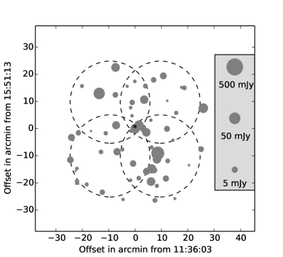
Figure 1.— Layout of the calibrator search pointings for the target PSR J1136$+$1551. Dashed lines show the 50% response level of the primary beam, and candidate calibrator sources from the FIRST survey are shown in grayscale.

The candidate sources were taken from the Faint Images of the Radio Sky (FIRST; Becker et al., 1995) catalog where available, and the NRAO VLA Sky Survey (NVSS; Condon et al., 1998) in areas not covered by FIRST. For future campaigns, the ongoing VLA Sky Survey (VLASS; Lacey et al. in prep.) will provide a deeper and higher resolution catalog covering the full NVSS footprint. Each pointing center was visited for approximately 3.5 minutes, which with an observing bandwidth of 64 MHz (dual polarization) gave a typical on-source root-mean-square (rms) noise of 0.3 mJy beam^-1–0.8 mJy beam^-1, depending on the location of the candidate in the pointing pattern. In general, this was sufficient to identify (at $>$6.5$\sigma$) any candidates within $\sim$25′ of the target pulsar brighter than 3 mJy (the completeness limit of NVSS) that could potentially serve as useful calibrators or astrometric check sources. The calibration and source detection approach was essentially the same as that used by the mJIVE-20 project (Deller & Middelberg, 2014), which was inspired by the procedure undertaken here.

These calibrator search observations for  served as a survey of over 200 square degrees at milliarcsecond resolution complete to $\sim$3 mJy, reliably detecting over 1500 sources. Over 90% of the 280 targeted pulsars were found to be located near at least one source suitable as a secondary phase calibrator for high-sensitivity observations (flux density $>$3 mJy contained within a component of maximum size several milliarcseconds, angular separation $<$25′).

From our initial sample of 280 pulsars, $\sim$110 met our requirements for astrometric observations with the then-available 512 Mbps recording system on the VLBA capable of recording dual polarization 64 MHz bandwidth. These requirements were: pulsar gated equivalent flux density $>$3.2 mJy, and at least one compact secondary calibrator within 25′ with flux density $>$6 mJy. We observed each of these 110 sources once using the astrometric scheme described in Section 2.2 below, before down-selecting to the final sample of 60 pulsars. The initial observations were used to reduce the risk of selecting a target where the final astrometric precision would be insufficient to provide a useful distance constraint. Some targets were rejected due to an unsuitable secondary calibrator, generally due to complicated source structure that was not identifed in the initial snapshot search observations due to limited $uv$ coverage. Other targets were rejected because that pulsar’s observed flux density was much fainter than the catalog value. Finally, from the remaining viable targets, preference was given to sources that sampled a range of Galactic longitudes and latitudes (which meant primarily discarding sources in the Galactic plane and located towards to inner Galaxy), and sources that did not already have a high-precision parallax distance. The final selection of 60 targets was therefore based on both logistical (range of right ascensions, strong calibrators close on the sky to the target, target flux density) and scientific (range of Galactic heights, predicted distances, individual objects where the distance was a high priority) considerations. The 60 selected sources are summarized in Table 1.

Table 1 targets

Pulsar	Pulsar	DM	S1.4g	Obs. Freq.	DNE2001	DYMW16
Jname	Bname	(pc cm-3)	(mJy)	(MHz)	(kpc)	(kpc)
J0040+5716	B0037+56	92.6	4.7	1660	3.05	2.42
J0055+5117	B0052+51	44.1	7.6	1660	1.90	1.94
J0102+6537	B0059+65	65.9	4.9	1660	2.29	1.98
J0108+6608	B0105+65	30.5	5.2	1660	1.42	1.46
J0147+5922	B0144+59	40.1	10.1	1660	2.22	1.58
J0151–0635	B0148–06	25.7	5.4	1660	1.22	25.00
J0152–1637	B0149–16	11.9	9.2	1660	0.51	0.92
J0157+6212	B0154+61	30.2	10.6	1660	1.71	1.39
J0323+3944	B0320+39	26.0	6.5	1660	1.01	1.20
J0332+5434	B0329+54	26.8	1244.9	1660	0.98	1.18
J0335+4555	B0331+45	47.2	4.6	1660	1.64	1.53
J0357+5236	B0353+52	103.7	6.1	1660	2.78	2.02
J0406+6138	B0402+61	65.3	13.5	1660	2.12	1.78
J0601–0527	B0559–05	80.5	11.8	1660	3.93	2.33
J0614+2229	B0611+22	96.9	12.5	1660	2.08	1.74
J0629+2415	B0626+24	84.2	17.9	1660	2.24	1.67
J0729–1836	B0727–18	61.3	8.0	1660	2.90	2.40
J0823+0159	B0820+02	23.7	8.3	1660	1.01	0.81
J0826+2637	B0823+26	19.5	76.4	1660	0.34	0.31
J1022+1001		10.3	9.5	1660	0.45	0.83
J1136+1551	B1133+16	4.9	181.9	1660	0.34	0.41
J1257–1027	B1254–10	29.6	7.3	1660	1.55	25.00
J1321+8323	B1322+83	13.3	4.3	1660	0.76	0.98
J1532+2745	B1530+27	14.7	4.8	1660	0.83	1.32
J1543–0620	B1540–06	18.4	15.2	1660	0.72	1.12
J1607–0032	B1604–00	10.7	26.2	1660	0.67	0.68
J1623–0908	B1620–09	68.2	4.7	1660	50.00	25.00
J1645–0317	B1642–03	35.7	167.4	1660	1.12	1.32
J1650–1654		43.2	8.7	1660	1.47	1.05
J1703–1846	B1700–18	49.6	4.8	1660	1.48	1.69
J1735–0724	B1732–07	73.5	9.5	1660	2.26	0.21
J1741–0840	B1738–08	74.9	6.5	1660	2.17	0.22
J1754+5201	B1753+52	35.4	9.3	1660	2.18	4.17
J1820–0427	B1818–04	84.4	37.9	2267	1.94	2.92
J1833–0338	B1831–03	234.5	18.8	2267	5.14	5.17
J1840+5640	B1839+56	26.7	25.0	1660	1.68	2.19
J1901–0906		72.7	20.4	1660	2.13	2.89
J1912+2104	B1910+20	88.3	7.4	1660	3.96	3.37
J1917+1353	B1915+13	94.5	10.4	2267	3.99	2.94
J1913+1400	B1911+13	145.1	7.3	2267	5.12	5.25
J1919+0021	B1917+00	90.3	5.7	1660	3.06	4.10
J1937+2544	B1935+25	53.2	7.7	1660	3.25	2.87
J2006–0807	B2003–08	32.4	8.8	1660	1.23	1.71
J2010–1323		22.2	5.8	1660	1.02	1.16
J2046–0421	B2043–04	35.8	12.7	1660	1.75	3.27
J2046+1540	B2044+15	39.8	10.5	1660	2.42	3.34
J2113+2754	B2110+27	25.1	8.9	1660	2.03	1.87
J2113+4644	B2111+46	141.3	62.9	1660	4.53	4.12
J2145–0750		9.0	21.2	1660	0.57	0.69
J2149+6329	B2148+63	128.0	11.0	1660	5.51	3.88
J2150+5247	B2148+52	148.9	8.6	1660	4.62	3.61
J2212+2933	B2210+29	74.5	3.8	1660	4.20	25.00
J2225+6535	B2224+65	36.1	10.0	1660	1.86	1.88
J2248–0101		29.1	4.6	1660	1.65	25.00
J2305+3100	B2303+30	49.5	17.2	1660	3.66	25.00
J2317+1439		21.9	10.3	1660	0.83	2.16
J2317+2149	B2315+21	20.9	6.5	1660	0.95	1.80
J2325+6316	B2323+63	197.4	6.7	1660	8.26	4.86
J2346–0609		22.5	8.2	1660	0.94	25.00
J2354+6155	B2351+61	94.7	31.6	1660	3.43	2.40

2.2. Astrometric observations

Each of the 232  astrometric epochs lasted $\sim$2.4 hours and targeted two pulsars located relatively close to each other on the sky, with typical angular separations of 10^∘–20^∘. In each observation, 5 fields were observed: the two target fields (each of which encompassed both a pulsar and one or more in-beam calibrators), two out-of-beam phase reference sources (one near each pulsar), and one strong “fringe finder” source used to calibrate the instrumental bandpass. The observing sequence was as follows:

• Five 5.5 minute scans on the first target field interleaved and bracketed by 1.25 minute scans on the associated primary calibrator;

• Five 5.5 minute scans on the second target field interleaved and bracketed by 1.25 minute scans on the associated primary calibrator;

• A two-minute scan on the fringe finder;

• Five 5.5 minute scans on the first target field interleaved and bracketed by 1.25 minute scans on the associated primary calibrator;

• Five 5.5 minute scans on the second target field interleaved and bracketed by 1.25 minute scans on the associated primary calibrator;

This observing sequence was used to ensure that the $uv$ coverage was maximised while keeping the slewing overheads relatively low.

In some cases, a known and suitable VLBI calibrator was separated by less than 25′ from the pulsar. In these cases, no nodding calibration was performed, reducing the observing block for that pulsar to a single 27.5 minute long scan (repeated twice during the observation).

The pointing center for the target fields was typically chosen to be close to the midpoint between the pulsar and the primary in-beam calibrator, although adjustments were made based on the location of additional in-beam calibrator sources in some cases. Figure 2 shows an example astrometric pointing layout for the target PSR J1136$+$1551, while https://safe.nrao.edu/vlba/psrpi/astrometric_pointings.html shows the pointing layout for all the target pulsars.

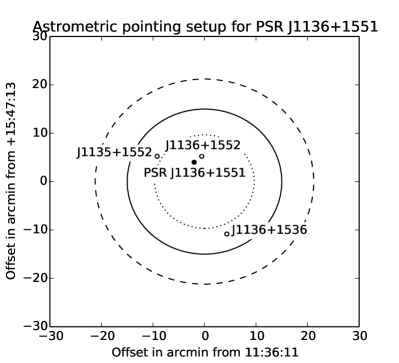
Figure 2.— The pointing layout of the target pulsar and in-beam calibrator sources for PSR J1136$+$1551. The dotted, solid and dashed lines show the 75%, 50% and 25% response contours of the primary beam at the center frequency of 1660 MHz.

The astrometric observations were scheduled during the period 2011 January to 2013 December, and were optimized in time to provide maximum sensitivity to annual geometric parallax. Since the VLBA is more extended in the east-west direction than north-south, the synthesized beam is narrower in right ascension than in declination. Accordingly, we scheduled our astrometric observations around the time of the peak parallax signature in right ascension. After the first “check” observation, every successive parallax extremum was sampled with two observations within a $\sim$20 day period. In total, each pulsar was observed 8 or 9 times spread over a $\sim$2 year period.

The observational setup consisted of four 16 MHz subbands, covering both circular polarizations and sampled at 2 bit precision for a total recording rate of 512 Mbps. In the first astrometric observation of each pulsar, the frequency range chosen was 1624.49 MHz–1688.49 MHz, while for the remaining observations the frequency range was shifted slightly to 1627.49 MHz–1691.49 MHz, due to strong interference from the Iridium satellite constellation at $\sim$1625 MHz. For four pulsars (PSRs J1820$-$0427, J1833$-$0338, J1913$+$1400, and J1917$+$1353), strong scatter-broadening led us to choose observations at higher frequency, 2234.49 MHz–2298.49 MHz. In the first observation of each pulsar, a significant portion of the data from the first subband was flagged due to this interference, while in the later observations, a lesser amount of data was flagged in the 4th subband due to interference at $\sim$1690 MHz.

Correlation was performed in Socorro using the DiFX software correlator (Deller et al., 2011). For each observation, a minimum of three and a maximum of six correlation passes were made, forming 3–6 separate visibility datasets. The first pass correlated all sources, using the position of the primary in-beam calibrator for scans on the target field. We refer to the resultant dataset henceforth as the “calibrator” dataset. All other passes correlated only the scans on the target fields, and differed in the location of the phase center and the presence or absence of special pulsar processing. The second pass used the position of the target pulsars and employed pulsar gating to boost the signal-to-noise (S/N) by down-weighting timeranges when the pulsar signal is weak or absent (Deller et al., 2007). The pulsar ephemeris and the pulsar gate parameters were obtained from timing observations with the Lovell telescope at Jodrell Bank Observatory. We refer to the output as the “gated” dataset. The third pass also used the position of the target pulsars, but used no pulsar gating, to generate the “ungated” dataset. Comparison of the S/N of the pulsar detection in the gated and ungated datasets allowed us to check that the correct pulsar ephemeris and gate had been applied. If present, the fourth, fifth, and sixth correlator passes used the position of the additional in-beam calibrator sources; we refer subsequently to these as the “additional” datasets.

2.3. Astrometric data calibration

In order to generate artifact-free images of the target pulsars that are located in a stable reference frame, careful calibration is needed to remove time- and frequency-dependent corruption of the measured visibilities by instrumental and propagation effects. All calibration was performed using AIPS (Greisen, 2003), facilitated by the ParselTongue python interface (Kettenis et al., 2006). AIPS version 31DEC15 was used for the final data processing, and each pulsar was processed independently. Calibration was script-based, with configurable options set using a markup-language control file for traceability. The cumulative calibration derived in the preceding stages is always applied before solving for the next stage of the incremental calibration. We now describe the calibration script stages in detail.

1. Load: The visibility datasets were loaded into AIPS using the task FITLD.

2. A priori flagging: Logged time ranges when the antennas are slewing, settling, or have otherwise known pointing or recording problems are already recorded in the flag table accompanying the dataset. In addition to these existing flags, we also flagged baselines during times when the natural fringe rate was low using the AIPS task UVFLG, as these are susceptible to corruption by radio frequency interference (RFI) and instrumental effects. We also flagged baselines when one or both antennas was pointing below 20^∘ elevation (AIPS task UVFLG). Finally, we applied any user-defined flags that were generated after inspection of final data products of an earlier pipeline run (AIPS task UVFLG).

3. Source shifting: If required, the phase center for one or more sources was shifted using the AIPS task CLCOR. This was typically only needed for the first observation, where the pulsar position was sometimes poorly known, and in some cases the in-beam calibrator position was also only poorly constrained after the initial snap-shot observation.

4. A priori ionosphere correction: The delay model applied at the correlator does not include any ionsospheric contribution. To correct for ionospheric propogation delays, we used the AIPS task TECOR, which makes use of a low-resolution global ionosphere model. While these global models are unable to remove rapid and/or small-scale variations, they do account for bulk ionospheric effects. We used the the final combined analysis models of the International GNSS Service (analysis center code igsg) available from ftp://cddis.gsfc.nasa.gov/gps/products/ionex/.

5. EOP corrections: The Earth Orientation Parameters (EOPs) used in the correlator model are often refined after the time of correlation. To update the visibilities and make use of the most accurate available EOPs in order to minimise residual position offsets after phase referencing, we used the AIPS task CLCOR.

6. A priori amplitude calibration: The visibilities in the correlator dataset are scaled to take the form of pseudo-correlation coefficients. To convert these to an approximate flux density scale in Janskys, the following steps are taken:

   1. Quantization correction: Imperfect level-setting in the quantizers bias the amplitude scale; this effect can be detected and corrected by analysis of the station autocorrelations. We used the AIPS task ACCOR to make these corrections.

   2. System temperature correction: A continuously operating switched noise diode at each VLBA antenna records the system temperature at that antenna. In combination with an a priori gain curve (which, at low frequencies such as used here, is quite accurate), this can be used to convert the pseudo-correlation coefficients produced by the correlator into Janskys. We use the AIPS task APCAL to generate these corrections.

   3. Primary beam correction: In the target pointing, the pulsar and in-beam calibrator(s) are not centered in the primary beam. Accordingly, the amplitude response for each of these sources is attenuated by the primary beam fall-off. We apply a correction based on a simplified model of a uniformly illuminated antenna scaled by the measured parameters for beam width and beam squint of VLBA antennas at our observing band, using a custom ParselTongue script described in Deller & Middelberg (2014).

7. Instrumental phase calibration: Any instrumental phase variations due to changing propagation through the signal chain are tracked by an injected pulse train, and the measured phases are stored in a table that accompanies the visibilities. We applied these corrections using the AIPS task PCCOR.

8. Time-independent delay calibration: Using the AIPS task FRING, we measured the single-band delays for each subband independently on the fringe finder source. A model of the fringe finder source derived from imaging the concatenated data for the source from all 8–9  epochs was supplied to FRING. The AIPS task SNSMO was used to apply a median window filter to the resultant delays and automatically exclude any solutions that differed by more than 10 nanoseconds from the median for that subband of that antenna. Rates were zeroed before the delays were applied using CLCAL.

9. Time-independent instrumental bandpass calibration: The AIPS task BPASS was used to derive the instrumental bandpass, using the fringe finder scan. As with the preceding step, the model of the fringe finder source was supplied to BPASS. The resultant amplitude corrections were normalized to leave the flux density scale unaffected.

10. Time-dependent delay calibration: We used the AIPS task FRING to now derive single-band delays using the phase reference calibrator source. Again, a source model (based on imaging of concatenated  datasets) was supplied in all cases. In almost all cases, each subband was solved separately, but for several weak phase reference sources, we combined all subbands together to improve the S/N. Solving for all subbands separately is preferred, because the residual ionospheric delays can lead to a (slightly) varying delay between subbands. When this is the case, approximating the delay as constant over all subbands reduces the S/N improvement resulting from the larger bandwidth, and also leaves per-subband phase residuals that must be corrected later. The solutions were median-window filtered using SNSMO to excise values where the delay or phase offsets exceeded 10 ns or 10 mHz, respectively.

11. Refinement of time-dependent amplitude calibration: The AIPS task CALIB was used to compute amplitude self-calibration corrections on a per-subband basis for the phase reference calibrator source, usually with a timescale of 20 minutes (shorter in some cases where the calibrator source was particularly strong). As in previous steps, the epoch-averaged calibrator model was employed, which in effect forces the absolute flux density scale to match this model. If the calibrator exhibited substantial flux density variations over the observing period, this could affect the flux density scale of individual observations; however, the absolute flux density scale is not important for the astrometric observables, which depend only on position. SNSMO was used to median-window filter and remove amplitude corrections differing by more than 20% from the median over the whole observation.

12. Refinement of time-dependent phase calibration in target direction: The following steps now made use of the strongest source(s) in the target pointing, with the results then being applied to all sources in the target pointing. In most cases, a single in-beam calibrator source was used to derive solutions. For some targets where no strong in-beam calibrator source was available, multiple in-beam sources were used together in a “multi-source selfcal” (Middelberg et al., 2013; Radcliffe et al., 2016). Finally, in several cases (PSR J0332+5434, PSR J1136+1551, and PSR J2113+4644), the pulsar itself was by far the strongest source in the field, and the gated pulsar dataset was used to derive these calibrations rather than one of the other in-beam sources.

    1. Frequency independent: The dataset(s) corresponding to the designated source(s) were split using the AIPS task SPLIT, to apply calibration and flagging and average the data in frequency for speed. For non-pulsar sources, the split dataset was then divided by the corresponding source model using the AIPS task UVSUB. If multiple in-beam sources were used in a “multi-source selfcal,” these normalized datasets were then combined with the AIPS task DBCON. CALIB was then used to solve for phase corrections on this normalized (and possibly concatenated) dataset, summing all subbands and polarizations. The solution interval ranged from 10 seconds for the brightest sources to 5 minutes for the weakest source, with a median value of 1.25 minutes.

    2. Frequency dependent: The preceding step was repeated, but this time treating frequency subbands separately while still summing polarizations. The reduced bandwidth per solution was compensated with a longer solution interval, typically 6 minutes–30 minutes. This step compensates for the small residual dispersive delays due to the ionosphere between the phase reference calibrator direction and the target direction.

13. Refinement of time-dependent amplitude calibration in target direction: For a handful of targets with sufficiently bright in-beam calibrators, we used CALIB to derive further self-calibration amplitude corrections using the in-beam calibrator data. SNSMO was applied to filter out solutions differing by more than 20% from the median.

14. Correction of pulsar scintillation: For some nearby pulsars, the scintles produced by diffractive scintillation in the interstellar medium are sufficiently large compared to our visibility resolution (diffractive timescale $\gg$ 1 second, diffractive bandwidth $\gg$ 1 MHz) that significant amplitude variations are apparent in the pulsar data. When significant diffractive scintillation was present, we derived time-dependent amplitude correction factors using a custom ParselTongue routine described in Deller et al. (2009). The solution interval was empirically determined by inspection of the uncorrected pulsar data.

15. Writing calibrated data: The fully calibrated datasets for the pulsar (both gated and ungated), the in-beam calibrator source(s), and the phase reference calibrator source were split and averaged to a single visibility point per frequency subband (excising the two edge channels). The non-pulsar sources were divided by the epoch-averaged source structure model, and all datasets (pulsar gated, pulsar ungated, calibrator sources, calibrator sources divided by model) were written to disk using the AIPS task FITTP.

16. Producing log files: While the script was running, statistics on the failure rates of each calibration step were retained. At the conclusion of the script, these are written into a summary webpage, along with any information from the VLBA operator’s log and plots of the delay, amplitude, and phase calibration tables generated by the script. Plots showing visibility amplitude as a function of baseline length are also generated for each source and included, to aid in the identification of unflagged RFI. If any evidence of RFI or unsatisfactory calibration was evident, then additional flagging was undertaken, and the calibration script was re-run.

2.4. Imaging and position extraction

After flagging, calibration, and averaging, the visibility data are now in a suitable form for the extraction of our astrometric observables. Given the calibration that has been applied, the pulsar is effectively being determined using the method of differential astrometry with respect to the position of the in-beam calibrators. Among the 73 in-beam calibrators, the positions of 14 were found in the Radio Fundamental Catalogue (RFC; Petrov & Kovalev, in preparation) derived using observations designed to improve the absolute positions of VLBI calibrator sources. The absolute positions of the other in-beam calibrators were determined with respect to the primary out-of-beam phase reference calibrators. For the out-of-beam calibrators, the RFC2019a solution was used, and the absolute positions listed in the RFC have coordinate uncertainties ranging from 0.1 to 0.9 mas (median: 0.18 mas). J2000 coordinates are used for all sources.

Rather than these uncertainties transferred from the out-of-beam calibrators, the absolute position uncertainties of the in-beam calibrators, and hence of the pulsars, is generally dominated by one of the following two factors:

1. A substantial angular separation from the out-of-beam calibrators to the target field, (up to $3.5^{\circ}$), leading to biases in position estimates when the calibration is extrapolated. At an observing frequency of 1600 MHz, the uncertainty depends strongly on the ionospheric conditions during the observation(s) as well as the size of the angular separation and the median observing elevation; a few mas is typical (Deller et al., 2016). We estimate this value for each pulsar field by examining the scatter in the in-beam positions obtained when imaging using only phase referencing from the out-of-beam calibrator (i.e., no self-calibration on the in-beam calibrator).

2. The frequency dependence of the core position of calibrator sources. The apparent core of calibrator sources, which defines their reference position, is determined from the region of peak brightness in an image. The true jet origin, the region at the jet apex, is invisible to an observer, as it is opaque (optical depth $\tau\gg 1$) due to synchrotron self-absorption. The apparent core is located where the jet becomes visible further away from the origin, when optical depth reaches $\tau\approx 1$ at the apparent jet base. The higher the frequency, the closer the observed core is to the jet apex. This effect is called the core-shift; more detailed descriptions can be found in, e.g., Marcaide & Shapiro (1984); Lobanov (1998); Kovalev et al. (2008); O’Sullivan & Gabuzda (2009); Voitsik et al. (2018); Pushkarev et al. (2019). According to Sokolovsky et al. (2011) the core-shift at 1600 MHz ranges from 0.6 to 2.4 mas with median 1.1 mas for a specially pre-selected sample of active galactic nuclei (AGN) jets with significant shifts. Pushkarev et al. (2012) has measured core-shifts for a large complete flux density limited sample beween 8 and 15 GHz and has found median values similar to Sokolovsky et al. (2011). Another complication arises with long-term core-shift variability, which can reach significant values of up to 1 mas between 2 and 8 GHz (Plavin et al., 2019). In this work we did not determine the core-shift, and thus the neglected core-shift introduces a $\sim$mas level bias in the chain of tying the pulsar position to the out-of-beam calibrator via an intermediate in-beam calibrator.

All three sources of uncertainty are added in quadrature when determining the absolute position uncertainty of the pulsar. However, none of these issues affect any shifts relative to the in-beam calibrator, which are relevant for determining proper motion and parallax. The contributions to the relative astrometric error budget are considered in more detail in Section 3.2.

For each visibility dataset (gated pulsar, ungated pulsar, calibrator source(s), and calibrator source(s) divided by their average model), we used the following procedure to extract a position, again implemented as a ParselTongue script. We loaded the dataset into the difmap package (Shepherd, 1997) and inverted the Stokes I visibility data to form a dirty image, using natural weighting. We then shifted the dataset to be approximately centered on the peak in the dirty image, and added a single point source component to the model at the location of the peak. We ran a model fit for 20 iterations, and then wrote the resultant clean image (pixel size 0.75 milliarcseconds) to disk in FITS format. This clean image was then loaded into AIPS and the position and position uncertainties were extracted with the task JMFIT to fit an elliptical gaussian, using a 20x20 pixel window centered on the peak. An example image, showing the fitted gaussian, best-fit position, and uncertainty, is shown in Figure 3.

In principle, position information can be extracted directly from the model fit, without the need to form an image and fit an elliptical gaussian. However, while the best-fit position is easily accessible, extracting a position uncertainty from a model fit is highly dependent on the overall scaling of the visibility weights. In contrast, the position uncertainty resulting from an image plane fit, where the root mean square fluctuations of a residual image can easily be measured, is well defined and robust under conditions that are typically satisfied for radio interferometric images (Condon, 1997). It is for this reason that we use JMFIT to extract positions and position uncertainties, although we did cross-check our astrometric results using the model-fit positions and estimated uncertainties, finding results that typically agreed to well within 1$\sigma$ (where the uncertainty was taken from the image plane fit.)

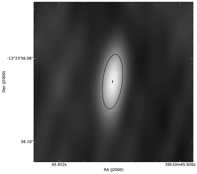
Figure 3.— A sample CLEAN image of a target pulsar, in this case PSR J2010$-$1323. Greyscale shows the sky brightness on a linear scale. The solid ellipse shows the best-fit gaussian returned by JMFIT, while the cross shows the best-fit position and associated uncertainty for the pulsar at this epoch. A detection with low signal-to-noise (S/N $\sim$ 16) was chosen to make the uncertainty bars visible.

2.5. Astrometric fitting

After the source modeling, calibration, and imaging described in the previous section was completed, we were left with a position time series for the target pulsar (taken from the higher S/N gated datasets) and one or more in-beam reference sources. The reference frame in which these positions were measured has been defined by the assumed positions for the source(s) used in step 12 of Section 2.3. This was not necessarily optimal for measuring the time-varying position of the target pulsar—the brightest in-beam calibrator might be located far from the pulsar, or might exhibit structure evolution that result in additional systematic errors. In these cases, we could provide a more stable reference frame by utilizing a weaker and/or more stable background source located at a smaller angular separation to the target pulsar.

By subtracting the position residuals from a given in-beam source (or a weighted average of several in-beam sources), we could transform the reference frame into one defined by an in-beam source (or sources) of our choosing. By selecting the source nearest to the target, it is possible to minimise the systematic position shifts at the target pulsar position introduced by the residual ionosphere. However, this also necessitates adding the formal fit errors for the chosen position reference source(s) in quadrature to the pulsar position fit error, which may not be an acceptable trade-off for weak background sources where these errors are large. Accordingly, for each pulsar we selected the position reference source considering both of these factors, and Table 2 shows the calibrator source(s) and the frame-defining source(s) for each target pulsar, along with the flux density as measured from the combined reference image for each source (at 1670 MHz for most sources, but at 2270 MHz for the calibrators of PSRs J1820$-$0427, J1833$-$0338, J1913$+$1400, and J1917$+$1353). Finally, any estimate of additional systematic sources of position uncertainty (see below) were added to the formal position errors; these were initially set to zero.

Table 2Calibrator sources for  targets.

Pulsar	Delay cal.	Sep.	Flux dens.	In-beam cal.	Sep.	Flux dens.	Position reference	Sep.	Flux dens.
		(∘)	(mJy)		(′)	(mJy)		(′)	(mJy)
J0040$+$5716	J0042$+$5708	0.3	910	J004219$+$570836	16.5	914	J004047$+$570321	13.2	7
J0055$+$5117	J0049$+$5128	1.0	180	J005620$+$512226	7.5	84	J005620$+$512226	7.5	84
J0102$+$6537	J0110$+$6805	2.6	400	J010225$+$653553	1.5	16	J010225$+$653553	1.5	16
J0108$+$6608	J0110$+$6805	2.0	400	J010845$+$660807	2.4	16	J010845$+$660807	2.4	16
J0147$+$5922	J0147$+$5840	0.7	210	J014921$+$592512	12.8	45	J014921$+$592512	12.8	45
J0151$-$0635	J0138$-$0540	3.2	270	J015230$-$062955	17.5	57	J015201$-$062904	11.4	12
J0152$-$1637	J0151$-$1732	0.9	180	J015325$-$163113	19.0	20	J015325$-$163113	19.0	20
J0157$+$6212	J0207$+$6246	1.2	1530	J015553$+$620701	14.6	63	J015553$+$620701	14.6	63
J0323$+$3944	J0322$+$3948	0.1	70	J032251$+$394802	7.4	72	J032251$+$394802	7.4	72
J0332$+$5434	J0346$+$5400	2.1	320	J0332$+$5434	0.0	1244	J033317$+$544011	6.1	7
J0335$+$4555	J0330$+$4656	1.3	220	J033346$+$460819	20.0	86	J033346$+$460819	20.0	86
J0357$+$5236	J0346$+$5400	2.2	320	J035751$+$524922	12.5	11	J035751$+$524922	12.5	11
				J035819$+$522936	9.0	12
J0406$+$6138	J0356$+$6043	1.5	180	J040635$+$611543	23.0	17	J040635$+$611543	23.0	17
J0601$-$0527	J0606$-$0724	2.3	410	J060250$-$053757	16.3	26	J060250$-$053757	16.3	26
J0614$+$2229	J0620$+$2102	2.0	870	J061411$+$222204	8.0	15	J061411$+$222204	8.0	15
J0629$+$2415	J0620$+$2102	3.8	870	J062909$+$235751	17.9	15	J062909$+$235751	17.9	15
J0729$-$1836	J0725$-$1904	1.0	230	J072831$-$182206	20.5	105	J072831$-$182206	20.5	105
J0823$+$0159	J0825$+$0309	1.3	420	J082344$+$020257	9.5	11	J082344$+$020257	9.5	11
J0826$+$2637	J0819$+$2747	2.0	240	J082733$+$263715	9.4	34	J082733$+$263715	9.4	34
J1022$+$1001	J1025$+$1253	3.0	470	J102334$+$101200	13.5	213	J102310$+$100126	3.2	18
J1136$+$1551	J1142$+$1547	1.5	160	J1136$+$1551	0.0	181	J113609$+$155228	1.9	15
J1257$-$1027	J1303$-$1051	1.6	270	J125751$-$101040	20.1	65	J125713$-$102403	3.8	4
J1321$+$8323	J1321$+$8316	0.1	390	J132145$+$831613	7.4	392	J132145$+$831613	7.4	392
J1532$+$2745	J1539$+$2744	1.7	140	J153330$+$273502	20.8	18	J153330$+$273502	20.8	18
J1543$-$0620	J1543$-$0757	1.6	1420	J154416$-$064253	25.0	33	J154416$-$064253	25.0	33
J1607$-$0032	J1557$-$0001	2.4	380	J160533$-$003106	24.7	36	J160533$-$003106	24.7	36
J1623$-$0908	J1624$-$0649	2.3	640	J162431$-$090255	19.3	12	J162431$-$090255	19.3	12
				J162414$-$092356	20.5	11	J162414$-$092356	20.5	11
J1645$-$0317	J1638$-$0340	1.7	330	J164410$-$031329	13.6	44	J164410$-$031329	13.6	44
J1650$-$1654	J1642$-$2007	3.8	100	J165133$-$170928	21.7	49	J165015$-$165730	4.0	24
J1703$-$1846	J1709$-$1728	1.9	410	J170441$-$185807	16.8	16	J170441$-$185807	16.8	16
				J170429$-$190336	19.6	16
J1735$-$0724	J1735$-$0559	1.4	530	J173401$-$071554	18.2	22	J173500$-$073321	8.5	8
				J173500$-$073321	8.5	8
J1741$-$0840	J1740$-$0811	0.6	170	J174002$-$083111	21.9	8	J174002$-$083111	21.9	8
J1754$+$5201	J1740$+$5211	2.1	1570	J175459$+$520114	5.7	19	J175459$+$520114	5.7	19
				J175550$+$520506	14.0	35
J1820$-$0427	J1819$-$0258	1.5	1480	J182043$-$042412	4.1	95	J182103$-$042633	3.0	29
				J182103$-$042633	3.0	29
J1833$-$0338	J1827$-$0405	1.5	510	J183323$-$032331	16.2	97	J183323$-$032331	16.2	97
J1840$+$5640	J1824$+$5651	2.3	630	J183849$+$564515	16.3	13	J183849$+$564515	16.3	13
J1901$-$0906	J1855$-$1209	3.4	140	J190252$-$085706	17.3	13	J190252$-$085706	17.3	13
				J190230$-$085144	17.2	15	J190230$-$085144	17.2	15
J1912$+$2104	J1908$+$2222	1.7	100	J191255$+$210734	4.1	30	J191255$+$210734	4.1	30
				J191326$+$205141	16.3	8	J191326$+$205141	16.3	8
J1917$+$1353	J1911$+$1611	2.7	490	J191718$+$140509	12.4	101	J191718$+$140509	12.4	101
J1913$+$1400	J1911$+$1611	2.2	490	J191324$+$140254	2.0	15	J191324$+$140254	2.0	15
J1919$+$0021	J1920$-$0236	3.0	320	J191851$+$002147	14.9	60	J191851$+$002147	14.9	60
J1937$+$2544	J1929$+$2543	1.6	210	J193805$+$253232	18.6	189	J193805$+$253232	18.6	189
J2006$-$0807	J2011$-$0644	1.9	2040	J200651$-$082625	21.3	78	J200651$-$082625	21.3	78
J2010$-$1323	J2011$-$1546	2.4	540	J201101$-$134359	20.4	34	J201101$-$134359	20.4	34
J2046$-$0421	J2055$-$0416	2.5	350	J204536$-$043534	15.4	56	J204536$-$043534	15.4	56
J2046$+$1540	J2045$+$1547	0.2	140	J204545$+$154727	14.7	135	J204545$+$154727	14.7	135
J2113$+$2754	J2114$+$2832	0.8	360	J211358$+$275059	12.4	68	J211312$+$275002	4.4	17
				J211312$+$275002	4.4	17
J2113$+$4644	J2123$+$4614	1.8	120	J2113$+$4644	0.0	62	J211432$+$463439	15.1	52
J2145$-$0750	J2142$-$0437	3.3	380	J214557$-$074748	3.1	20	J214557$-$074748	3.1	20
J2149$+$6329	J2148$+$6107	2.4	1460	J215159$+$633527	14.6	13	J215159$+$633527	14.6	13
J2150$+$5247	J2201$+$5048	2.6	530	J214842$+$525403	18.4	12	J214842$+$525403	18.4	12
J2212$+$2933	J2205$+$2926	1.4	140	J221207$+$293356	3.6	77	J221207$+$293356	3.6	77
J2225$+$6535	J2238$+$6804	2.8	100	J222346$+$654751	17.9	16	J222346$+$654751	17.9	16
				J222417$+$652805	12.4	6	J222417$+$652805	12.4	6
J2248$-$0101	J2247$+$0000	1.1	450	J224808$-$011532	14.5	36	J224808$-$011532	14.5	36
J2305$+$3100	J2307$+$3230	1.5	400	J230655$+$305028	15.5	39	J230655$+$305028	15.5	39
J2317$+$1439	J2327$+$1524	2.6	190	J231619$+$143511	12.8	23	J231619$+$143511	12.8	23
				J231715$+$145130	12.1	17
J2317$+$2149	J2318$+$2404	2.3	130	J231657$+$220241	19.0	15	J231657$+$220241	19.0	15
				J231643$+$220626	23.9	94
J2325$+$6316	J2302$+$6405	2.6	110	J232445$+$633001	13.5	9	J232519$+$631636	0.8	5
				J232519$+$631636	0.8	5
J2346$-$0609	J2348$-$0425	1.8	240	J234636$-$060813	3.8	6	J234636$-$060813	3.8	6
				J234728$-$060526	10.4	9
J2354$+$6155	J2339$+$6010	2.5	310	J235440$+$613736	18.7	54	J235440$+$613736	18.7	54

This time series of measured positions and estimated uncertainties could then be processed using the pmpar package to perform least-squares minimization and fit for reference position, proper motion, and parallax. Four of the  targets are a pulsar in a binary system, and where the orbital reflex motion is substantial additional steps were required in the fitting process. PSR J1022$+$1001 and PSR J2145$-$0750 are millisecond pulsars that have already been described in Deller et al. (2016), while PSR J0823$+$0159 is a slow pulsar in a long-period binary. For these pulsars, the orbital period, longitude of periastron, eccentricity, and projected semi-major axis were all well-constrained by pulsar timing, and we therefore were only required to fit for inclination $i$ and longitude of ascending node $\Omega$. For PSR J2317+1439, the orbital reflex motion is negligible compared to our positional uncertainties. For the pulsars where fitting the orbital reflex motion was required, we included these two additional parameters in our least-squares minimization.

In almost all of the  pulsars, the reduced $\chi^{2}$ of the initial least-squares fit exceeded unity, often considerably. This result is not surprising given that the initial input position uncertainties are purely based on the S/N of the pulsar (and position reference calibrator) images, and do not account for potential systematic position shifts. In most cases, the dominant systematic contribution comes from the residual unmodeled ionosphere, but other possibilities such as source structure evolution in the source(s) defining the reference frame also exist. In general, the distribution (both form and variance) of these systematic errors is extremely difficult to predict a priori, as discussed in Section 3.2, which complicates efforts to accurately estimate the uncertainties on the fitted astrometric parameters. The problem is exacerbated for datasets where the formal position uncertainties vary widely between epochs, as can be the case for pulsars that exhibit significant amplitude variability due to diffractive and/or refractive scintillation. If no adjustment is made to the formal position errors, then the epochs with high-significance detections when the pulsar was “scintillated up” will exhibit a disproportionate impact on the astrometric fit.

In Section 3.2, we investigate different methods for estimating a systematic error that can be added in quadrature to the formal position fit errors in order to mitigate this issue. Unsurprisingly, we find that no method is perfect in all situations, but that the use of an estimator is better than neglecting systematic errors entirely. Our final astrometric solutions therefore make use of the empiral systematic error estimator discussed in Section 3.2.

Once a position time series with final estimated uncertainties is available, best-fit values and uncertainties for the astrometric parameters must be produced. Two options are available:

1. A simple least squares fit; or

2. A bootstrap fit.

The least-squares fit has the advantage of simplicity, but is sensitively dependent on beginning with a good estimate of the input position errors. If these are underestimated (which will generally result in a reduced $\chi^{2}$ that still significantly exceeds unity) then the errors on the astrometric observables will likewise be underestimated. Conversely (but more rarely), overestimating the systematic errors will lead to inflated uncertainties on the astrometric observables. A bootstrap fit (e.g., Efron & Tibshirani, 1991) utilizes a large number of trials, where in each trial $N$ position measurements for the input dataset for each trial are selected randomly with replacement from the available $N$ astrometric position measurements for that pulsar. In our case, $N$ is usually 8 or 9. For each trial dataset, a least-squares fit is made as usual, and the best-fit parameters are saved. After many trials, a cumulative probability distribution for each of the fitted parameters is built, from which the most probable value and a desired confidence interval can be extracted.

A bootstrap fit has the advantage that the uncertainty on the fitted parameters is not determined solely by the uncertainty in the input position measurements, which as we have seen is hard to estimate accurately. However, the bootstrap approach can exacerbate a problem already present for  and most VLBI astrometry programs: the small sample size. With just 8 or 9 position measurements, a significant fraction of trials can end up with poor time coverage of one of the desired astrometric quantities, sampling a shorter time range or predominantly one side of the parallax signature. This is especially problematic in cases where the pulsar scintillates and is detected only weakly (or not at all) in some epochs, further reducing the number of useful degrees of freedom. An example is PSR J2317$+$1439, where non-detections due to unfavourable scintillation were concentrated in the December/January observations and resulted in a poor sampling of the parallax ellipse.

We favor a bootstrap approach for determining the final astrometric uncertainties, as it generally produces the most conservative error estimates (as can be seen in Section 3.2). The results presented here are obtained from a bootstrap with 100,000 trials per pulsar. We highlight the circumstances under which the bootstrap uncertainties may potentially be too conservative in the discussion.

3. Results

3.1. Astrometric fits for 60 pulsars

The astrometric results for our 60 target pulsars are shown in Table LABEL:tab:allresults. Asymmetric error bars representing the 68% confidence interval are listed along with the best-fit parameter values. The median parallax uncertainty obtained was 46 $\mu$as, with 60% of our targets meeting or exceeded the design goal of 50 $\mu$as parallax accuracy. Almost all (53 of the 60) target pulsars have a significant ($>$95% confidence) parallax measurement, while two-thirds of the sample provide a distance error of 20% or less.

Detailed results, including astrometric plots and calibrator images, can be found for each pulsar at https://safe.nrao.edu/vlba/psrpi/release.html. As an example, the astrometric plots and bootstrap histograms for PSR J0601$-$0527 are shown in Figure 4. This is a typical-to-challenging target—the signal-to-noise ratio on the target was $\sim$50, and the in-beam calibrator was slightly resolved, with a total flux density of $\sim$25 mJy, and separated from the target by 16′. The reduced $\chi^{2}$ of the astrometric fit to the position time series using the empirical systematic error estimate discussed in Section 3.2 is 1.3, and the attained parallax precision of $\sim$40 $\mu\mathrm{as}$ is very close to the median  value.

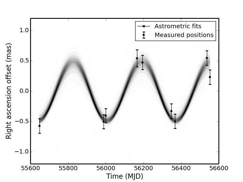
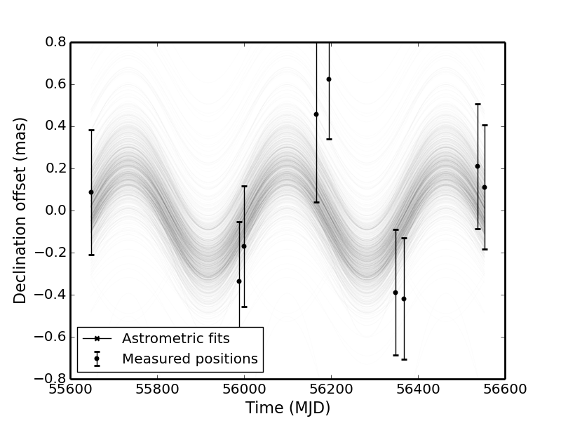
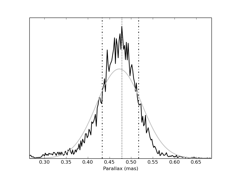
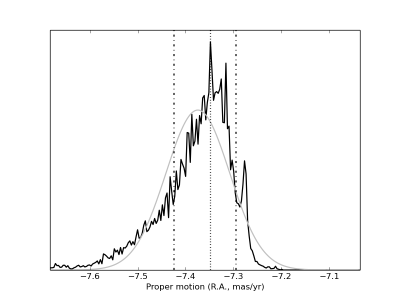
Figure 4.— Top: Illustration of the bootstrap fits for PSR J0601$-$0527, showing position offset in right ascension (left) and declination (right) after subtraction of the best-fit proper motion. Each of the 100,000 fits is overplotted in a light greyscale, and so darker regions indicate the most likely parallax signature. Bottom: Probability distribution functions for parallax (left) and proper motion in right ascension (right). The black line shows the results of the bootstrap which are used in the text, while for comparison purposes, a light grey line shows the result of a least-squares fit after adding additional systematic error contributions to obtain a reduced $\chi^{2}$ of 1.0.

Table 3Fitted astrometric parameters for all PSR$\pi$ targets. Position offsets are relative to the defined position for the chosen reference source, at epoch MJD 56000.0; the right ascension offset is calculated at the declination of the target pulsar.

Pulsar	Offset from reference		Proper motion		Parallax
	R.A.	Decl.	R.A.	Decl.
	(mas)	(mas)	(mas/yr)	(mas/yr)	(mas)
J0040+5716	$-119735.120^{+0.037}_{-0.045}$	$783183.975^{+0.064}_{-0.109}$	$12.399^{+0.033}_{-0.057}$	$-5.450^{+0.140}_{-0.082}$	$0.102^{+0.051}_{-0.025}$
J0055+5117	$-332840.251^{+0.071}_{-0.023}$	$-302297.263^{+0.085}_{-0.074}$	$10.490^{+0.049}_{-0.085}$	$-17.352^{+0.074}_{-0.204}$	$0.349^{+0.055}_{-0.055}$
J0102+6537	$47321.472^{+0.074}_{-0.006}$	$79472.077^{+0.041}_{-0.045}$	$9.252^{+0.049}_{-0.081}$	$1.828^{+0.093}_{-0.206}$	$0.399^{+0.044}_{-0.045}$
J0108+6608	$-140564.314^{+0.039}_{-0.033}$	$27077.203^{+0.050}_{-0.025}$	$-32.754^{+0.036}_{-0.025}$	$35.162^{+0.024}_{-0.051}$	$0.468^{+0.035}_{-0.031}$
J0147+5922	$-744046.103^{+0.100}_{-0.038}$	$-189510.613^{+0.093}_{-0.054}$	$-6.380^{+0.083}_{-0.101}$	$3.826^{+0.054}_{-0.097}$	$0.495^{+0.042}_{-0.093}$
J0151-0635	$-582099.427^{+0.164}_{-0.014}$	$-358146.639^{+0.066}_{-0.052}$	$10.697^{+0.094}_{-0.145}$	$-5.373^{+0.061}_{-0.078}$	$0.217^{+0.098}_{-0.076}$
J0152-1637	$-1067819.606^{+0.158}_{-0.014}$	$-399877.713^{+0.363}_{-0.330}$	$0.804^{+0.234}_{-0.201}$	$-31.372^{+0.424}_{-0.313}$	$0.443^{+0.214}_{-0.181}$
J0157+6212	$814250.347^{+0.035}_{-0.007}$	$325456.249^{+0.037}_{-0.010}$	$1.521^{+0.105}_{-0.017}$	$44.811^{+0.034}_{-0.048}$	$0.554^{+0.039}_{-0.024}$
J0323+3944	$401715.413^{+0.046}_{-0.011}$	$-189856.218^{+0.029}_{-0.017}$	$26.484^{+0.059}_{-0.034}$	$-30.780^{+0.029}_{-0.015}$	$1.051^{+0.039}_{-0.040}$
J0332+5434	$-158517.350^{+0.035}_{-0.008}$	$-328076.504^{+0.050}_{-0.029}$	$16.969^{+0.027}_{-0.029}$	$-10.379^{+0.058}_{-0.036}$	$0.595^{+0.020}_{-0.025}$
J0335+4555	$939470.468^{+0.073}_{-0.010}$	$-746024.523^{+0.066}_{-0.058}$	$-3.638^{+0.023}_{-0.073}$	$-0.097^{+0.134}_{-0.105}$	$0.409^{+0.022}_{-0.027}$
J0357+5236	$-61073.169^{+0.128}_{-0.028}$	$-744690.138^{+0.062}_{-0.089}$	$13.908^{+0.062}_{-0.115}$	$-10.633^{+0.098}_{-0.058}$	$0.305^{+0.029}_{-0.077}$
J0406+6138	$-41240.544^{+0.050}_{-0.171}$	$1377882.120^{+0.122}_{-0.093}$	$12.400^{+0.151}_{-0.085}$	$22.716^{+0.100}_{-0.060}$	$0.218^{+0.051}_{-0.057}$
J0601-0527	$-765952.497^{+0.074}_{-0.014}$	$606395.795^{+0.097}_{-0.144}$	$-7.348^{+0.053}_{-0.077}$	$-15.227^{+0.084}_{-0.105}$	$0.478^{+0.039}_{-0.045}$
J0614+2229	$81743.228^{+0.050}_{-0.021}$	$471984.943^{+0.062}_{-0.014}$	$-0.233^{+0.036}_{-0.053}$	$-1.224^{+0.011}_{-0.065}$	$0.282^{+0.022}_{-0.031}$
J0629+2415	$-54102.959^{+0.179}_{-0.041}$	$1069457.665^{+0.054}_{-0.047}$	$3.629^{+0.050}_{-0.193}$	$-4.607^{+0.013}_{-0.153}$	$0.333^{+0.036}_{-0.054}$
J0729-1836	$862898.001^{+0.143}_{-0.043}$	$-875533.906^{+0.400}_{-0.390}$	$-13.072^{+0.125}_{-0.091}$	$13.252^{+0.456}_{-0.418}$	$0.489^{+0.098}_{-0.078}$
J0823+0159	$-525441.078^{+0.150}_{-0.134}$	$-225189.223^{+0.080}_{-0.095}$	$-3.797^{+0.073}_{-0.415}$	$0.171^{+0.232}_{-0.281}$	$0.376^{+0.129}_{-0.070}$
J0826+2637	$-566289.704^{+0.007}_{-0.007}$	$5345.818^{+0.072}_{-0.012}$	$62.994^{+0.021}_{-0.007}$	$-96.733^{+0.045}_{-0.085}$	$2.010^{+0.013}_{-0.009}$
J1022+1001	$-190717.466^{+0.043}_{-0.016}$	$25883.813^{+0.039}_{-0.025}$	$-14.921^{+0.050}_{-0.033}$	$5.611^{+0.033}_{-0.035}$	$1.387^{+0.041}_{-0.028}$
J1136+1551	$-87829.834^{+0.010}_{-0.016}$	$-73945.169^{+0.047}_{-0.031}$	$-73.785^{+0.031}_{-0.010}$	$366.569^{+0.072}_{-0.055}$	$2.687^{+0.018}_{-0.016}$
J1257-1027	$-135426.468^{+0.059}_{-0.059}$	$-182136.895^{+0.087}_{-0.066}$	$-7.164^{+0.140}_{-0.105}$	$12.079^{+0.119}_{-0.110}$	$0.141^{+0.064}_{-0.092}$
J1321+8323	$36.330^{+0.115}_{-0.070}$	$446008.090^{+0.173}_{-0.130}$	$-52.674^{+0.099}_{-0.076}$	$32.373^{+0.204}_{-0.048}$	$0.968^{+0.036}_{-0.140}$
J1532+2745	$-1068597.478^{+0.106}_{-0.029}$	$646805.042^{+0.113}_{-0.118}$	$1.542^{+0.082}_{-0.127}$	$18.932^{+0.104}_{-0.118}$	$0.624^{+0.031}_{-0.096}$
J1543-0620	$-690701.998^{+0.041}_{-0.008}$	$1328301.506^{+0.120}_{-0.113}$	$-16.774^{+0.026}_{-0.063}$	$-0.312^{+0.147}_{-0.114}$	$0.322^{+0.028}_{-0.045}$
J1607-0032	$1476474.720^{+0.060}_{-0.014}$	$-94965.170^{+0.163}_{-0.266}$	$-26.437^{+0.027}_{-0.099}$	$-27.505^{+0.222}_{-0.200}$	$0.934^{+0.026}_{-0.047}$
J1623-0908	$-1100560.359^{+0.175}_{-0.043}$	$-352982.390^{+0.182}_{-0.097}$	$-10.769^{+0.131}_{-0.120}$	$23.509^{+0.166}_{-0.069}$	$0.586^{+0.101}_{-0.099}$
J1645-0317	$770570.904^{+0.016}_{-0.016}$	$-268070.730^{+0.107}_{-0.136}$	$-1.011^{+0.003}_{-0.051}$	$20.523^{+0.147}_{-0.205}$	$0.252^{+0.028}_{-0.019}$
J1650-1654	$172228.769^{+0.061}_{-0.006}$	$168064.225^{+0.097}_{-0.056}$	$-15.024^{+0.002}_{-0.092}$	$-6.556^{+0.148}_{-0.131}$	$-0.089^{+0.031}_{-0.015}$
J1703-1846	$-717146.582^{+0.047}_{-0.025}$	$712491.475^{+0.182}_{-0.194}$	$-0.751^{+0.102}_{-0.056}$	$16.962^{+0.146}_{-0.230}$	$0.348^{+0.049}_{-0.047}$
J1735-0724	$61924.490^{+0.076}_{-0.043}$	$508913.404^{+0.087}_{-0.093}$	$0.791^{+0.087}_{-0.029}$	$20.614^{+0.074}_{-0.046}$	$0.150^{+0.041}_{-0.035}$
J1741-0840	$1190194.661^{+0.112}_{-0.069}$	$-560681.159^{+0.066}_{-0.087}$	$0.436^{+0.082}_{-0.126}$	$6.876^{+0.109}_{-0.066}$	$0.279^{+0.050}_{-0.058}$
J1754+5201	$-341736.402^{+0.074}_{-0.010}$	$-1983.221^{+0.056}_{-0.083}$	$-3.950^{+0.047}_{-0.046}$	$1.101^{+0.072}_{-0.059}$	$0.160^{+0.029}_{-0.022}$
J1820-0427	$-169381.766^{+0.076}_{-0.027}$	$-63903.822^{+0.120}_{-0.109}$	$-7.318^{+0.074}_{-0.055}$	$15.883^{+0.088}_{-0.069}$	$0.351^{+0.049}_{-0.055}$
J1833-0338	$269293.573^{+0.119}_{-0.060}$	$-932810.642^{+0.182}_{-0.260}$	$-17.409^{+0.158}_{-0.025}$	$15.038^{+0.333}_{-0.337}$	$0.408^{+0.050}_{-0.067}$
J1840+5640	$945467.477^{+0.053}_{-0.011}$	$-260360.747^{+0.070}_{-0.029}$	$-31.212^{+0.033}_{-0.022}$	$-29.079^{+0.047}_{-0.082}$	$0.657^{+0.065}_{-0.008}$
J1901-0906	$-880884.264^{+0.071}_{-0.014}$	$-543910.907^{+0.113}_{-0.163}$	$-7.531^{+0.034}_{-0.045}$	$-18.211^{+0.143}_{-0.159}$	$0.510^{+0.067}_{-0.042}$
J1912+2104	$-170443.421^{+0.121}_{-0.006}$	$-180675.561^{+0.070}_{-0.085}$	$-11.335^{+0.023}_{-0.097}$	$-5.768^{+0.092}_{-0.122}$	$0.024^{+0.171}_{-0.022}$
J1913+1400	$-6337.234^{+0.050}_{-0.018}$	$-122121.054^{+0.047}_{-0.033}$	$-5.265^{+0.040}_{-0.072}$	$-8.927^{+0.038}_{-0.065}$	$0.185^{+0.027}_{-0.023}$
J1917+1353	$316294.074^{+0.016}_{-0.016}$	$-672694.400^{+0.039}_{-0.025}$	$-1.253^{+0.022}_{-0.074}$	$3.811^{+0.057}_{-0.064}$	$0.142^{+0.068}_{-0.007}$
J1919+0021	$893781.316^{+0.091}_{-0.045}$	$-7819.701^{+0.060}_{-0.083}$	$10.167^{+0.029}_{-0.143}$	$-4.713^{+0.102}_{-0.073}$	$0.166^{+0.042}_{-0.042}$
J1937+2544	$-865965.163^{+0.039}_{-0.015}$	$700670.139^{+0.029}_{-0.039}$	$-10.049^{+0.042}_{-0.030}$	$-13.055^{+0.034}_{-0.039}$	$0.318^{+0.031}_{-0.029}$
J2006-0807	$-522282.331^{+0.076}_{-0.010}$	$1163967.750^{+0.184}_{-0.126}$	$-6.176^{+0.035}_{-0.070}$	$-10.616^{+0.174}_{-0.123}$	$0.424^{+0.010}_{-0.101}$
J2010-1323	$-225966.545^{+0.305}_{-0.205}$	$1202928.433^{+0.188}_{-0.146}$	$2.358^{+0.329}_{-0.210}$	$-5.611^{+0.257}_{-0.303}$	$0.484^{+0.166}_{-0.120}$
J2046+1540	$777607.703^{+0.099}_{-0.016}$	$-413782.623^{+0.041}_{-0.072}$	$-10.455^{+0.032}_{-0.090}$	$0.681^{+0.039}_{-0.090}$	$0.310^{+0.082}_{-0.076}$
J2046-0421	$357981.097^{+0.006}_{-0.037}$	$848678.492^{+0.105}_{-0.268}$	$10.760^{+0.038}_{-0.035}$	$-4.404^{+0.373}_{-0.076}$	$0.167^{+0.026}_{-0.042}$
J2113+2754	$-109967.706^{+0.033}_{-0.005}$	$238352.997^{+0.047}_{-0.058}$	$-27.981^{+0.052}_{-0.014}$	$-54.432^{+0.040}_{-0.096}$	$0.704^{+0.023}_{-0.022}$
J2113+4644	$-704691.944^{+0.078}_{-0.025}$	$569536.867^{+0.066}_{-0.029}$	$9.525^{+0.068}_{-0.148}$	$8.846^{+0.076}_{-0.090}$	$0.454^{+0.077}_{-0.065}$
J2145-0750	$-111529.383^{+0.076}_{-0.016}$	$-149818.403^{+0.054}_{-0.080}$	$-9.491^{+0.052}_{-0.042}$	$-9.114^{+0.090}_{-0.076}$	$1.603^{+0.063}_{-0.009}$
J2149+6329	$-809671.242^{+0.101}_{-0.027}$	$-343634.854^{+0.184}_{-0.072}$	$15.786^{+0.131}_{-0.082}$	$11.255^{+0.092}_{-0.284}$	$0.356^{+0.072}_{-0.061}$
J2150+5247	$1041961.339^{+0.176}_{-0.105}$	$-373619.769^{+0.163}_{-0.179}$	$8.377^{+0.226}_{-0.181}$	$-4.427^{+0.247}_{-0.353}$	$0.034^{+0.164}_{-0.081}$
J2212+2933	$207796.901^{+0.052}_{-0.052}$	$-50710.117^{+0.050}_{-0.083}$	$-5.513^{+0.067}_{-0.102}$	$-11.322^{+0.102}_{-0.128}$	$0.265^{+0.050}_{-0.120}$
J2225+6535	$782263.168^{+0.201}_{-0.065}$	$-735020.424^{+0.050}_{-0.058}$	$147.220^{+0.243}_{-0.223}$	$126.532^{+0.076}_{-0.115}$	$1.203^{+0.166}_{-0.204}$
J2248-0101	$279160.561^{+0.151}_{-0.010}$	$824047.754^{+0.184}_{-0.083}$	$-10.548^{+0.117}_{-0.027}$	$-17.407^{+0.110}_{-0.267}$	$0.256^{+0.049}_{-0.067}$
J2305+3100	$-733995.388^{+0.042}_{-0.009}$	$572881.368^{+0.078}_{-0.068}$	$-3.737^{+0.082}_{-0.006}$	$-15.571^{+0.049}_{-0.163}$	$0.223^{+0.033}_{-0.028}$
J2317+1439	$721838.143^{+0.100}_{-1.295}$	$259459.178^{+0.827}_{-0.829}$	$-1.476^{+0.465}_{-0.065}$	$3.806^{+0.272}_{-0.704}$	$0.603^{+1.533}_{-0.241}$
J2317+2149	$834190.412^{+0.040}_{-0.056}$	$-773795.695^{+0.093}_{-0.101}$	$8.522^{+0.035}_{-0.104}$	$0.136^{+0.192}_{-0.084}$	$0.510^{+0.057}_{-0.049}$
J2325+6316	$-45049.774^{+0.080}_{-0.012}$	$16351.365^{+0.149}_{-0.083}$	$-5.926^{+0.082}_{-0.073}$	$-2.051^{+0.188}_{-0.192}$	$-0.010^{+0.049}_{-0.043}$
J2346-0609	$203020.882^{+0.037}_{-0.006}$	$-106887.144^{+0.060}_{-0.052}$	$37.390^{+0.025}_{-0.042}$	$-20.230^{+0.107}_{-0.070}$	$0.275^{+0.021}_{-0.036}$
J2354+6155	$-253697.746^{+0.058}_{-0.005}$	$1090745.164^{+0.035}_{-0.019}$	$22.755^{+0.056}_{-0.040}$	$4.888^{+0.033}_{-0.016}$	$0.412^{+0.031}_{-0.043}$

The fitted parallax and proper motion results can be used to derive distances, Galactic z-heights, and transverse velocities for the target pulsars, or lower limits in the case where the parallax was not measured to sufficient accuracy. Likewise, the fitted offsets from the inbeam calibrators can be combined with an estimate of the in-beam calibrator position uncertainty (comprising contributions from core-shift, phase-referencing to the out-of-beam calibrator, and the out-of-beam calibrator absolute uncertainty added in quadrature as described in Section 2.4), to produce an absolute pulsar position at the reference epoch and associated uncertainty. All of these derived quantities are shown in Table LABEL:tab:derivedresults. We stress that the absolute positions are of a preliminary nature, since the calibrator positions and core-shifts have not been determined to high precision, and note in particular that the positional uncertainties for PSR J0614+2229, PSR J0629+2415, and PSR J1820-0427 could be substantially underestimated due to the fact that their out-of-beam calibrator source exhibits a compact double structure.

The most probable distance and the 68% confidence interval were calculated directly from the fitted parallax and confidence interval, without applying any priors based on an assumed pulsar spatial distribution or luminosity distribution (e.g., Verbiest et al., 2012; Igoshev et al., 2016). For high-significance parallax detections, the distance is relatively insensitive to the assumed priors, but we note that for low significance parallax detections (for instance, the 20  pulsars with a parallax significance below 5 $\sigma$) the inferred distance can be substantially dependent on the assumed priors. The most probable transverse velocity was estimated using the most probable distance and most probable proper motion, while the 68% confidence interval was calculated by finding the smallest rectangular cuboid in (parallax, proper motion (R.A.), proper motion (Decl.)) space that encompassed 68% of the bootstrap trial results, and taking the highest and lowest transverse velocity from these included trials. Figure 5 shows an example of the transverse velocity estimator for PSR J0601$-$0527.

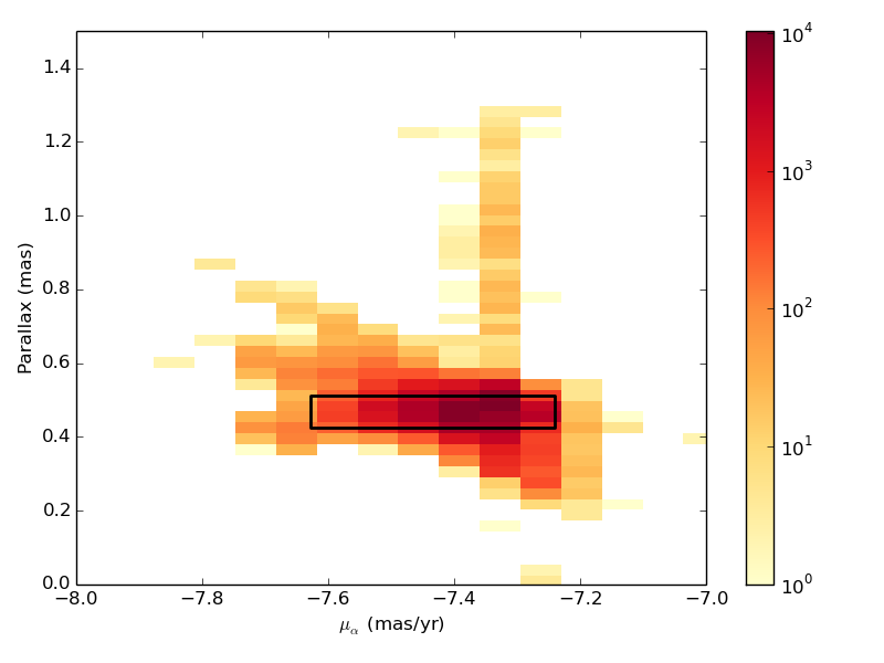
Figure 5.— Probability density maps for parallax vs proper motion in right ascension (left) and parallax vs proper motion in declination (right) for PSR J0601$-$0527. The dark rectangles on the plot show the projections of the cuboid selected for estimating the 68% confidence interval for transverse velocity. The smallest cuboid contains the most compact 70% interval along the parallax axis, the most compact 98.5% interval along the proper motion (R.A.) axis, and the most compact 97% interval along the proper motion (Dec.) axis, which collectively retains 68% of the bootstrap trials.

Table 4Derived astrometric parameters for all PSR$\pi$ targets. Positions are shown at the reference epoch of MJD 56000.0. 1$\sigma$ uncertainties are shown on measured values (parentheses show uncertainties on the last digit), and lower limits are shown with 95% confidence.

Pulsar	Right Ascension	Declination	Dist.	z-height	Trans. vel.
	(J2000)	(J2000)	(kpc)	(kpc)	(km/s)
J0040+5716	00:40:32.3899(1)	+57:16:24.833(1)	$9.77^{+3.13}_{-3.23}$	$0.95^{+0.30}_{-0.31}$	$626.3^{+203.2}_{-221.5}$
J0055+5117	00:55:45.3981(1)	+51:17:24.601(1)	$2.87^{+0.54}_{-0.39}$	$0.58^{+0.11}_{-0.08}$	$275.7^{+56.0}_{-42.5}$
J0102+6537	01:02:32.9914(1)	+65:37:13.416(1)	$2.51^{+0.32}_{-0.25}$	$0.12^{+0.02}_{-0.01}$	$111.9^{+16.5}_{-12.9}$
J0108+6608	01:08:22.5049(3)	+66:08:34.499(1)	$2.14^{+0.15}_{-0.15}$	$0.12^{+0.01}_{-0.01}$	$487.0^{+36.4}_{-35.2}$
J0147+5922	01:47:44.6434(1)	+59:22:03.284(1)	$2.02^{+0.46}_{-0.16}$	$0.10^{+0.02}_{-0.01}$	$71.1^{+17.4}_{-6.6}$
J0151$-$0635	01:51:22.7179(2)	$-$06:35:02.987(2)	$4.60^{+2.45}_{-1.43}$	$4.17^{+2.22}_{-1.30}$	$261.0^{+116.8}_{-93.4}$
J0152$-$1637	01:52:10.8539(1)	$-$16:37:53.641(2)	$2.26^{+1.56}_{-0.73}$	$2.15^{+1.48}_{-0.70}$	$335.8^{+219.4}_{-124.4}$
J0157+6212	01:57:49.9434(1)	+62:12:26.648(1)	$1.80^{+0.08}_{-0.12}$	$0.01^{+0.00}_{-0.00}$	$383.7^{+17.8}_{-25.8}$
J0323+3944	03:23:26.6619(1)	+39:44:52.403(1)	$0.95^{+0.04}_{-0.03}$	$0.24^{+0.01}_{-0.01}$	$183.2^{+7.6}_{-7.0}$
J0332+5434	03:32:59.4096(1)	+54:34:43.329(1)	$1.68^{+0.07}_{-0.06}$	$0.04^{+0.00}_{-0.00}$	$158.6^{+7.5}_{-5.6}$
J0335+4555	03:35:16.6416(1)	+45:55:53.452(1)	$2.44^{+0.18}_{-0.12}$	$0.34^{+0.02}_{-0.02}$	$42.2^{+5.7}_{-2.4}$
J0357+5236	03:57:44.8403(2)	+52:36:57.493(1)	$3.27^{+1.10}_{-0.29}$	$0.03^{+0.01}_{-0.00}$	$271.7^{+93.1}_{-30.4}$
J0406+6138	04:06:30.0806(2)	+61:38:41.408(1)	$4.58^{+1.63}_{-0.87}$	$0.56^{+0.20}_{-0.11}$	$562.8^{+212.6}_{-107.7}$
J0601$-$0527	06:01:58.9752(2)	$-$05:27:50.871(4)	$2.09^{+0.22}_{-0.16}$	$0.49^{+0.05}_{-0.04}$	$167.8^{+23.8}_{-13.4}$
J0614+2229	06:14:17.0058(1)	+22:29:56.848(1)	$3.55^{+0.44}_{-0.26}$	$0.15^{+0.02}_{-0.01}$	$21.0^{+4.3}_{-2.3}$
J0629+2415	06:29:05.7273(1)	+24:15:41.546(1)	$3.00^{+0.57}_{-0.29}$	$0.33^{+0.06}_{-0.03}$	$84.0^{+19.0}_{-11.6}$
J0729$-$1836	07:29:32.3369(1)	$-$18:36:42.244(2)	$2.04^{+0.39}_{-0.34}$	$0.01^{+0.00}_{-0.00}$	$179.9^{+40.7}_{-36.5}$
J0823+0159	08:23:09.7651(1)	+01:59:12.469(1)	$2.66^{+0.60}_{-0.68}$	$0.96^{+0.22}_{-0.25}$	$47.8^{+18.9}_{-11.8}$
J0826+2637	08:26:51.5068(1)	+26:37:21.297(1)	$0.50^{+0.00}_{-0.00}$	$0.26^{+0.00}_{-0.00}$	$272.3^{+1.3}_{-1.9}$
J1022+1001	10:22:57.9957(1)	+10:01:52.765(2)	$0.72^{+0.01}_{-0.02}$	$0.56^{+0.01}_{-0.02}$	$54.5^{+1.3}_{-2.0}$
J1136+1551	11:36:03.1198(1)	+15:51:14.183(1)	$0.37^{+0.00}_{-0.00}$	$0.35^{+0.00}_{-0.00}$	$659.7^{+4.2}_{-4.5}$
J1257$-$1027	12:57:04.7625(2)	$-$10:27:05.551(2)	$7.09^{+13.18}_{-2.22}$	$5.62^{+10.44}_{-1.76}$	$474.1^{+886.4}_{-160.0}$
J1321+8323	13:21:45.6315(7)	+83:23:39.432(1)	$1.03^{+0.17}_{-0.04}$	$0.57^{+0.10}_{-0.02}$	$302.6^{+51.6}_{-12.0}$
J1532+2745	15:32:10.3646(1)	+27:45:49.623(1)	$1.60^{+0.29}_{-0.07}$	$1.31^{+0.24}_{-0.06}$	$144.0^{+28.8}_{-7.6}$
J1543$-$0620	15:43:30.1373(1)	$-$06:20:45.332(2)	$3.11^{+0.51}_{-0.25}$	$1.85^{+0.30}_{-0.15}$	$247.4^{+41.3}_{-22.2}$
J1607$-$0032	16:07:12.0598(2)	$-$00:32:41.527(2)	$1.07^{+0.06}_{-0.03}$	$0.62^{+0.03}_{-0.02}$	$193.4^{+13.0}_{-7.0}$
J1623$-$0908	16:23:17.6599(1)	$-$09:08:48.733(2)	$1.71^{+0.34}_{-0.25}$	$0.78^{+0.16}_{-0.12}$	$209.4^{+44.0}_{-34.3}$
J1645$-$0317	16:45:02.0406(1)	$-$03:17:57.819(2)	$3.97^{+0.33}_{-0.39}$	$1.74^{+0.14}_{-0.17}$	$386.4^{+38.7}_{-43.2}$
J1650$-$1654	16:50:27.1694(7)	$-$16:54:42.282(20)	$>$ 3.1	$>$ 0.9	$>$ 229.8
J1703$-$1846	17:03:51.0915(2)	$-$18:46:14.845(6)	$2.88^{+0.45}_{-0.36}$	$0.67^{+0.11}_{-0.08}$	$231.5^{+40.4}_{-38.6}$
J1735$-$0724	17:35:04.9730(1)	$-$07:24:52.130(1)	$6.68^{+2.03}_{-1.43}$	$1.53^{+0.47}_{-0.33}$	$653.1^{+205.8}_{-144.8}$
J1741$-$0840	17:41:22.5629(1)	$-$08:40:31.711(1)	$3.58^{+0.94}_{-0.55}$	$0.70^{+0.18}_{-0.11}$	$116.7^{+35.7}_{-21.8}$
J1754+5201	17:54:22.9068(1)	+52:01:12.244(1)	$6.27^{+1.03}_{-0.98}$	$3.10^{+0.51}_{-0.48}$	$122.0^{+22.4}_{-22.2}$
J1820$-$0427	18:20:52.5934(1)	$-$04:27:37.712(2)	$2.85^{+0.52}_{-0.35}$	$0.23^{+0.04}_{-0.03}$	$236.0^{+47.0}_{-30.2}$
J1833$-$0338	18:33:41.8945(1)	$-$03:39:04.258(1)	$2.45^{+0.48}_{-0.27}$	$0.10^{+0.02}_{-0.01}$	$266.7^{+56.8}_{-34.0}$
J1840+5640	18:40:44.5372(1)	+56:40:54.852(1)	$1.52^{+0.02}_{-0.14}$	$0.62^{+0.01}_{-0.06}$	$307.9^{+5.2}_{-27.8}$
J1901$-$0906	19:01:53.0087(3)	$-$09:06:11.146(10)	$1.96^{+0.17}_{-0.23}$	$0.22^{+0.02}_{-0.03}$	$183.1^{+20.4}_{-24.3}$
J1912+2104	19:12:43.3391(1)	+21:04:33.926(1)	$41.02^{+377.75}_{-35.90}$	$3.57^{+32.86}_{-3.12}$	$2482.4^{+6732.3}_{-2184.1}$
J1913+1400	19:13:24.3527(1)	+14:00:52.559(1)	$5.42^{+0.75}_{-0.70}$	$0.15^{+0.02}_{-0.02}$	$266.3^{+39.5}_{-37.6}$
J1917+1353	19:17:39.7864(1)	+13:53:57.077(1)	$7.04^{+0.38}_{-2.29}$	$0.08^{+0.00}_{-0.02}$	$134.5^{+9.7}_{-47.8}$
J1919+0021	19:19:50.6715(1)	+00:21:39.722(2)	$6.03^{+2.02}_{-1.21}$	$0.65^{+0.22}_{-0.13}$	$319.6^{+107.2}_{-72.3}$
J1937+2544	19:37:01.2544(1)	+25:44:13.436(1)	$3.15^{+0.32}_{-0.28}$	$0.12^{+0.01}_{-0.01}$	$245.9^{+25.1}_{-24.4}$
J2006$-$0807	20:06:16.3650(1)	$-$08:07:02.167(3)	$2.36^{+0.73}_{-0.06}$	$0.82^{+0.25}_{-0.02}$	$137.1^{+45.4}_{-8.5}$
J2010$-$1323	20:10:45.9211(1)	$-$13:23:56.083(4)	$2.07^{+0.68}_{-0.53}$	$0.83^{+0.27}_{-0.21}$	$58.7^{+26.9}_{-16.0}$
J2046+1540	20:46:39.3373(1)	+15:40:33.558(1)	$3.22^{+1.04}_{-0.68}$	$0.93^{+0.30}_{-0.20}$	$160.0^{+48.2}_{-35.4}$
J2046$-$0421	20:46:00.1730(1)	$-$04:21:26.256(2)	$5.98^{+2.00}_{-0.81}$	$2.75^{+0.92}_{-0.37}$	$329.3^{+112.3}_{-50.6}$
J2113+2754	21:13:04.3506(1)	+27:54:01.160(1)	$1.42^{+0.04}_{-0.04}$	$0.34^{+0.01}_{-0.01}$	$412.1^{+14.2}_{-13.8}$
J2113+4644	21:13:24.3295(1)	+46:44:08.844(1)	$2.20^{+0.36}_{-0.32}$	$0.05^{+0.01}_{-0.01}$	$135.8^{+18.4}_{-24.8}$
J2145$-$0750	21:45:50.4588(1)	$-$07:50:18.514(4)	$0.62^{+0.00}_{-0.02}$	$0.42^{+0.00}_{-0.02}$	$38.9^{+0.5}_{-1.9}$
J2149+6329	21:49:58.7033(2)	+63:29:44.277(2)	$2.81^{+0.58}_{-0.47}$	$0.36^{+0.07}_{-0.06}$	$258.3^{+52.6}_{-49.4}$
J2150+5247	21:50:37.7499(1)	+52:47:49.556(1)	$>$ 2.4	$>$ 0.0	$>$ 89.1
J2212+2933	22:12:23.3444(1)	+29:33:05.411(1)	$3.77^{+3.14}_{-0.60}$	$1.40^{+1.16}_{-0.22}$	$225.7^{+193.8}_{-38.2}$
J2225+6535	22:25:52.8627(3)	+65:35:36.371(1)	$0.83^{+0.17}_{-0.10}$	$0.10^{+0.02}_{-0.01}$	$765.2^{+157.6}_{-94.5}$
J2248$-$0101	22:48:26.8859(1)	$-$01:01:48.085(1)	$3.90^{+1.40}_{-0.63}$	$3.02^{+1.08}_{-0.49}$	$377.1^{+149.2}_{-66.7}$
J2305+3100	23:05:58.3212(1)	+31:00:01.281(1)	$4.47^{+0.65}_{-0.58}$	$2.01^{+0.29}_{-0.26}$	$341.1^{+56.4}_{-47.2}$
J2317+1439	23:17:09.2364(1)	+14:39:31.265(1)	$1.66^{+1.10}_{-1.19}$	$1.12^{+0.74}_{-0.80}$	$31.4^{+30.0}_{-22.9}$
J2317+2149	23:17:57.8419(1)	+21:49:48.019(1)	$1.96^{+0.21}_{-0.20}$	$1.16^{+0.12}_{-0.12}$	$79.3^{+8.9}_{-9.6}$
J2325+6316	23:25:13.3196(2)	+63:16:52.362(1)	$>$ 12.1	$>$ 0.4	$>$ 327.8
J2346$-$0609	23:46:50.4978(1)	$-$06:09:59.899(2)	$3.64^{+0.55}_{-0.26}$	$3.27^{+0.50}_{-0.23}$	$732.5^{+114.5}_{-53.1}$
J2354+6155	23:54:04.7830(1)	+61:55:46.845(1)	$2.42^{+0.28}_{-0.17}$	$0.01^{+0.00}_{-0.00}$	$268.0^{+32.7}_{-20.3}$

3.2. Analysing the astrometric error budget

As shown above, correctly estimating the total uncertainty of the position measurements used for the astrometric fit is challenging. Below, we summarise the primary contributions to the error budget:

1. Thermal noise in the target image: This is the most readily quantified, as it can be easily extracted from the image-plane fitting. It is inversely proportional to the instrumental resolution and inversely proportional to the signal-to-noise in the pulsar image. This term generally dominates for faint sources.

2. Systematic offsets introduced by differential propagation effects between the target and calibrator: This is usually the dominant term for bright sources, where the signal-to-noise on the target is not the limiting factor. At 1600 MHz, the ionosphere dominates these path length differences, which vary on a sub-epoch timescale (minutes to hours). The solutions on the calibrator must be extrapolated spatially to the target, and are averaged over a time interval during which the ionosphere can change. Generally, the spatial extrapolation introduces the largest error, meaning this term is most dependent on the calibrator-target separation, along with factors influencing the mean path length through the ionosphere such as the solar activity level, time of day, and antenna elevation. The amount of temporal averaging required depends on the calibrator flux density and structure – for a typical 20 mJy calibrator, a solution interval of order 1.25 minutes was typical.

   Refraction in the interstellar medium also produces a differential offset between a pulsar and calibrator. For the  sample, the predicted angular wandering (using the predictions of the NE2001 model and assuming a Kolmogorov density spectrum; Cordes & Lazio, 2002) at the observing frequency (1660 or 2270 MHz) for our target pulsars due to refraction has a median value for a given observation of $\sim 0.05$ mas. For most pulsars, this is a negligible component of the astrometric error. However, the predicted scattering disk diameter exceeds 1 mas and the predicted refractive wander exceeds 0.1 mas for four pulsars in our sample: PSR J0601$-$0527, PSR J1833$-$0338, PSR J2212+2933, and PSR J2325+6313. In cases such as these, and others where the astrometric precision is extremely high, refractive wander of the pulsar may be a significant component of the error budget.

   As well as the pulsar, refractive wander also affects the in-beam calibrator sources, which is another potential source of error in the target–calibrator separation. Generally, the refractive wander is larger for calibrators than for the pulsars, as the radiation from the calibrators passes by all of the Galactic electrons along the line of sight, leading to a larger scattering disk. For PSR J1833$-$0338, for instance, the NE2001 model predicts refractive wander with an rms deviation of 0.4 mas for the position reference calibrator source, nearly three times larger than that of the pulsar. However, the refractive wander timescale for the calibrator sources is typically much longer (years), meaning that reference position will be affected more than proper motion, which will itself be affected more than parallax.

3. Systematic variations in the image reference frame: An imperfect model of the calibrator source will lead to an offset in the obtained pulsar position. If this is constant in time, it does not impact the measurement of parallax or proper motion, but time variability is an important source of error. Time variability could be the result of evolution intrinsic to the source itself (which is present, at least at a low level, in all compact sources), or from changes in the observing setup (different frequency or $uv$ coverage between observing epochs). This can be the dominant term if the calibrator source is bright and close to the target (minimizing the ionospheric terms) but is a blazar-like source which displays large and rapid variations in the jet structure. Over the 1 yr–2 yr timescale typical for pulsar astrometry programs such as , it is often possible to fit a significant component of this reference source offset with a linear function with time, meaning it can corrupt the proper motion measured for the pulsar. However, for most reference sources the likely effect is small compared to our measurement error (the median apparent proper motion seen by Moór et al., 2011, was 19 $\mu\mathrm{as}$ yr^-1, versus 106 $\mu\mathrm{as}$ yr^-1 for our relative astrometric uncertainty), and parallax (which has a sinusoidal signature with time) is much less affected. As well as effects intrinsic to the source, time-variable position shifts due to the changing Galactic gravitational potential field can be expected (Larchenkova et al., 2017), albeit only at the level of up to $\sim$10 $\mu\mathrm{as}$ over our timescales, and hence smaller than the reference source structure effects.

4. Stochastic noise in the image reference frame: The phase solutions on the calibrator source will have some noise dependent on the signal-to-noise in each solution interval, which is determined by the source flux density, instrumental sensitivity, and calibration interval. Fainter calibrators will generally lead to an increase in this term; although this could be compensated by increasing the solution interval, that would be reduce the ability to compensate for time-variable ionospheric effects. Changing the solution interval can thus shift error between this term and term 2 above; we seek to choose a value on a per-source basis that minimises their sum.

Accordingly, there are five main factors we would expect to influence the total uncertainty of a position measurement in a given epoch:

1. Pulsar flux density

2. Calibrator flux density

3. Pulsar-calibrator angular separation

4. Ionospheric conditions and average observing elevation

5. Calibrator stability

We can straightforwardly measure all but the last of these factors, and as noted the calibrator stability is not usually expected to be a significant contributor to the total error budget. We undertook a number of approaches to try and determine the contributions of each of the remaining factors to our error budget. To illustrate the results, we again use the typical-to-challenging source PSR J0601$-$0527, where the thermal noise errors alone substantially underestimate the total error budget, as can be seen from the reduced $\chi^{2}\sim 15$ for a simple least-squares fit to the unmodified position data.

First, we examined the apparent shifts in pulsar position within an observation, by subdividing the data into two halves and imaging each one separately. This approach is particularly useful for identifying observations where short-term ionospheric conditions were unstable—if the two positions differ by considerably more than their formal error bars, it is likely that the mean position over the whole observation also has an underestimated position uncertainty. However, while reliable, this approach is likely not complete, as it would fail to pick up observations with large but relatively stable residual ionospheric “wedges” that lead to a fairly constant position offset over the whole observation duration. Also, when the target source is faint, making a significant measurement of the offset between the two halves of the observation may not be possible.

We evaluated an approach in which we recorded the minimum systematic offset between the two observation halves (accounting for the uncertainty in the position measurements) and set the systematic error contribution to the whole epoch to be half of this value. The right ascension and declination axes are treated separately. The effect, as expected, was to lower the chi-squared of the resultant astrometric fit, although the position errors remained underestimated (as determined by a $\chi^{2}$ value well in excess of 1.0) in many cases. Figure 6 shows the result for PSR J0601$-$0527. As expected, this approach yields a systematic error estimate that is too low; the reduced $\chi^{2}$ remains at 10. Using this refined position set as the input for bootstrap fits results in a change in the best-fit value at the 1$\sigma$ level, and gives a small reduction in the estimated parameter uncertainty. For most targets, the impact on both best-fit value and uncertainty was smaller than in this example.

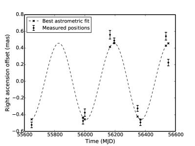
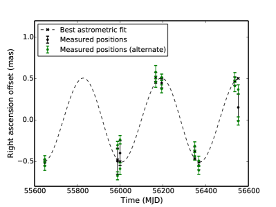
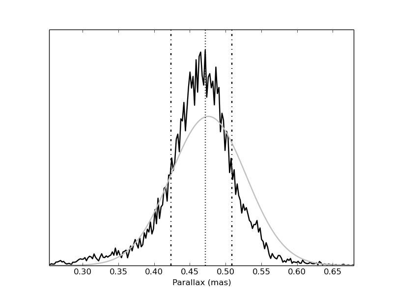
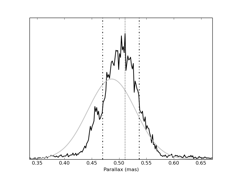
Figure 6.— The effect of including an estimate of the systematic error based on apparent positional wander during an observation for PSR J0601$-$0527. The plots in the first row show the offset in right ascension as a function of time, after subtracting the best-fit proper motion. Top left: least-squares fit to dataset without systematic errors. The reduced $\chi^{2}$ is 15. Top right: least squares fit to dataset including systematic error estimate. The measurements with error bars in green show the positions obtained from each half-observation—these are not fit, but show the size of the potential systematic offserts. The reduced $\chi^{2}$ is 10. Bottom left: the bootstrap fit results for parallax, from the dataset without systematic error estimates. The parallax obtained is $0.47\pm 0.04$ mas. Bottom right: the bootstrap fit results for parallax, from the dataset with systematic error estimates. The parallax obtained is $0.51^{+0.03}_{-0.04}$ $\mu$as.

Second, we processed the datasets multiple times making use of different ionospheric models, and examined the resultant position scatter for each epoch. If different ionospheric models of comparable quality give widely divergent positions, then the residual error from our chosen ionospheric model is likely high, since we have no way of determining which of the ionospheric models is correct. As with the previous approach comparing the two halves of an observation in time, this method is likely reliable but not necessarily complete, since it will not pick up cases where all models suffer from the same deficiencies.

We investigated all of the products covering our complete observing timespan from ftp://cddis.gsfc.nasa.gov/gps/products/ionex/, and found that the jplg, codg, igsg, and esag models consistently gave the best results, with the lowest residuals on the astrometric fit. The igsg model was chosen for the final data reduction. We therefore trialed an appoach in which, for every epoch, we computed the rms scatter in the positions provided by processing using these 4 models, and used this as the estimate for systematic error for that epoch. As with the epoch-splitting approach above, the right ascension and declination axes were treated separately. We found that for many sources, a given ionospheric model yielded a statistically significant mean offset across all epochs in addition to random scatter, and so for all sources we subtracted (per model) the mean positional offset from all epochs before computing the rms.

As expected and as with the previous approach splitting the observation in halves, and as expected, we typically capture some but not all of the systematic error with this technique. Figure 7 shows the result for PSR J0601$-$0527; the reduced $\chi^{2}$ is still 8. The best-fit value for parallax changes by approximately 0.2$\sigma$, and the estimated parallax uncertainty from the bootstrap fit is reduced by $\sim$10%.

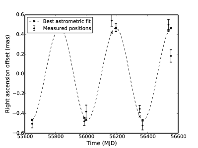
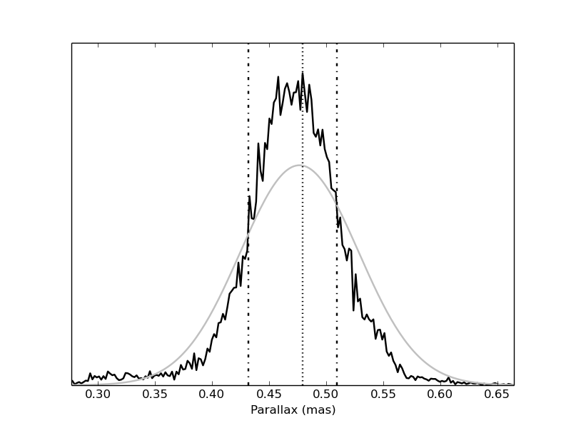
Figure 7.— The effect of including an estimate of the systematic error based on the scatter between ionospheric models for PSR J0601$-$0527. Left: least-squares fit to dataset with systematic error estimates included: offset in right ascension is shown as a function of time, after subtracting the best-fit proper motion. The reduced $\chi^{2}$ is 8. Right: the bootstrap fit results for parallax, from the dataset with systematic error estimates. The parallax obtained is $0.47\pm 0.04$ $\mu$as.

Our third approach to estimate systematic error made use of the residual position errors across our entire data set of 60 pulsars. As shown above, we expect the dominant error sources to depend on the calibrator-target separation, the observing elevation, and the calibrator brightness. As a simplification, we consider that the systematic error should be proportional to two quantities: the mean “deprojected” calibrator-target separation (calculated as the angular separation multiplied by the cosecant of the observing elevation, averaged over all antennas and all scans in the observation) and the signal-to-noise ratio achieved on the inbeam calibrator source(s). For each epoch, we added a systematic error estimate given by:

$$\Delta_{\mathrm{sys}}=A\times\frac{s\times\sum_{a=1}^{N}\sum_{o=1}^{M}\mathrm{cosec}\left(\mathrm{el_{a,o}}\right)}{M\times N}+B/S$$ (1)

where $\Delta_{\mathrm{sys}}$ is the systematic error estimate in fractions of a synthesized beam, $s$ is the calibrator-target separation in arcminutes, $\mathrm{el}_{a,o}$ is the observing elevation for antenna $a$ in scan $o$ on the target pulsar, $N$ and $M$ are the number of antennas and target scans respectively, and $S$ is the signal-to-noise ratio on the calibrator source (added in quadrature if multiple sources were used). We conducted a brute-force grid search for the optimal values of the coefficients $A$ and $B$, seeking the values that gave the tightest grouping of reduced $\chi^{2}$ values around 1.0 for our ensemble of 60 target pulsars.

The optimal values were found to be $A=0.001$, $B=0.6$. When this estimate of systematic error is added for all pulsars, the 25%, median, and 75% values of reduced $\chi^{2}$ across all pulsars becomes 0.64,1.08, and 1.69, compared to 1.78, 4.81, and 11.96 when no estimate of systematic error is added. The spread in reduced $\chi^{2}$ values is comparable to that expected given the typical number of degrees of freedom ($\sim$11) in the astrometric fits. The results for our example pulsar PSR J0601$-$0527 are shown in Figure 8; the typical systematic error contribution is 110 $\mu\mathrm{as}$ in right ascension and 280 $\mu\mathrm{as}$ in declination at each epoch, and the revised reduced $\chi^{2}$ is 1.35.

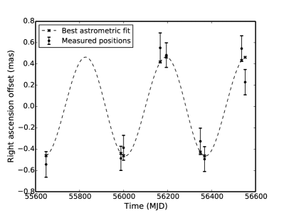
Figure 8.— The effect of including an empirical estimate of the systematic error based on the calibrator-target separation and calibrator flux density. Left: least-squares fit to dataset with systematic error estimates included: offset in right ascension is shown as a function of time, after subtracting the best-fit proper motion. The reduced $\chi^{2}$ is 1.4. Right: the bootstrap fit results for parallax, from the dataset with systematic error estimates. The parallax obtained is $0.48\pm 0.04$ $\mu$as.

We summarise the results of our different estimates of systematic error for PSR J0601$-$0527 in Table 5. Three things are immediately apparent:

1. The inclusion of systematic error (however estimated) pushes the estimated parallax in one direction. When the position errors are severely underestimated (as they are initially), individual discrepant epochs can have overly large effects on the fit. This diminishes once a more realistic error is applied.

2. The fitted parameters and their uncertainties remain relatively unchanged regardless of the systematic error estimate used when estimated using a bootstrap.

3. The fitted parameters and their uncertainties exhibit good agreement between a bootstrap and a simple least-squares fit when the systematic errors are reasonably well estimated (as appears to be the case for the empirically estimated values).

For our quoted results, we choose to use the bootstrap fit to the dataset including empirically estimated systematic errors, which is generally the most conservative (and we believe) correct error estimate we can make with our available information. We do however note that in some cases, generally when the parallax has been poorly sampled due to non-detections, this bootstrap error estimate may be overly conservative (since many trials have effectively no sensitivity to parallax). In these cases, better constraints could be obtained by interpreting, with caution, the least-squares fit to the dataset incorporating empirically estimated systematic errors. We highlight this for individual pulsars in the discussion that follows in Section 4.1.

Table 5Comparison between systematic error estimators

Estimator	Reduced $\chi^{2}$	Change in fitted	Relative parallax
		parallax (mas)	uncertainty
None	15.2	0.000	1.00
Time division	10.2	0.029	0.79
Ionosphere	7.8	0.010	0.91
Empirical	1.4	0.013	0.99

Finally, since the unmodeled ionosphere dominates the error budget in many cases, we should expect that the level of solar activity should significantly impact the results obtained. While the solar cycle peaking in 2013 was not particularly active by historical standards, our observations were nevertheless made near the solar maximum, and accordingly we would expect that the same observations repeated a half-decade later would yield better results. Likewise, the precise results seen in, e.g., Deller et al. (2012) and Deller et al. (2013) might have been more difficult to obtain at the time of the observations presented here. Importantly, our empirical estimates of systematic error should be used with caution when applied to observations in different observing conditions. An even larger observing program might consider including a measure of ionospheric activity as a parameter in the empirical fit to account for this.

4. Discussion

4.1. Notes on individual pulsars

From our sample of 60 pulsars, three sources display discrepancies which indicate a potentially biased parallax estimation. We consider the results for these sources in detail and estimate the probability that any of the remaining 57 sources have comparable but undetected errors.

4.1.1 PSR J1650–1654

PSR J1650–1654 has a significant negative parallax of $-0.089^{+0.030}_{-0.019}$ mas (where the uncertainty denotes the 68% confidence interval from the bootstrap fit). Since a negative parallax is unphysical, this indicates that the obtained value is incorrect by at least 3$\sigma$, but possibly more as the NE2001 distance obtained using the pulsar’s dispersion measure is just 1.5 kpc.

Two in-beam calibration sources are present, allowing us to cross-check results. The relative position separation of the in–beam phase calibrator source J165133–170928 from the second in-beam source J165015–165730 displays quite a large scatter (0.2 mas rms in right ascension, 0.25 mas rms in declination, as seen in Figure 9), and an astrometric fit to this relative separation time series gives a best-fit parallax of 0.05 mas with an uncertainty of $\sim$0.1 mas. This is not unexpected given the differential ionosphere across the $\sim 20$′ separation. However, as shown in Figure 9, the position reference J165015–165730 is separated by just 4′ from the pulsar, meaning that differential ionospheric effects should be smaller than between the two calibrators. An alternative is that the position reference source J165015–165730 exhibits substantial structure variations that lead to position offsets up to a few tenths of a milliarcsecond between epochs, and a substantial amount of the power this introduces into the pulsar’s position time series can be fit by the parallax term. The structure of the two calibrator sources can be seen in Figure 9 – both exhibit prominent milliarcsecond-scale jets, meaning structure evolution is likely at some level.

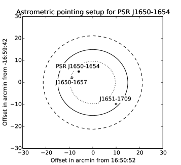
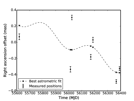
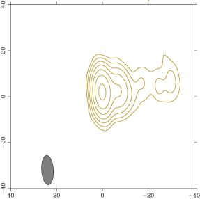
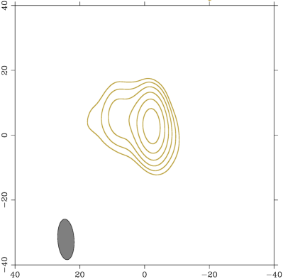
Figure 9.— Top left: The pointing layout of the target pulsar and in-beam calibrator sources for PSR J1650–1654. The dotted, solid and dashed lines show the 75%, 50% and 25% response point of the primary beam at the center frequency of 1650 MHz. Top right: relative offset between the two calibrator sources – error bars show measurements and the dashed line shows the best fit. Bottom left: In-beam phase calibrator source J165133–170928, where the axis scale is milliarcseconds from the reference position. Bottom right: Position reference source J165015–165730.

At present, we have no definitive explanation for the discrepant parallax for PSR J1650–1654, but the results indicate that the parallax uncertainty is underestimated by a factor of several for this pulsar.

4.1.2 PSR J1820–0427

PSR J1820–0427 has two in-beam calibrator sources (J182043–042412 and J182103–042633), which are close to each other and to the pulsar on the sky (angular separations 3′ – 5′). PSR J1820–0427 was observed at 2.3 GHz due to the strong scattering along this low Galactic latitude line of sight.

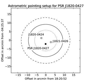
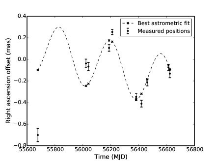
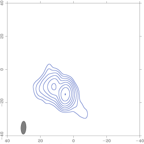
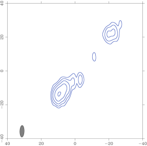
Figure 10.— Top left: The pointing layout of the target pulsar and in-beam calibrator sources for PSR J1820–0427. The dotted, solid and dashed lines show the 75%, 50% and 25% response point of the primary beam at the center frequency of 2360 MHz. Top right: relative offset between the two calibrator sources – error bars show measurements and the dashed line shows the best fit. Bottom left: In-beam phase calibrator source J182043–042412, where the axis scale is milliarcseconds from the reference position. Bottom right: In-beam phase calibrator and position reference source J182103–042633.

Figure 10 shows the clear structure in the residuals between the two in–beam calibrators. The large offset in the first observation is likely due to the different observing frequency (1650 MHz vs 2360 MHz), which would result in a different observed source structure. Neglecting this, however, it is clear that a significant parallax is measured between the two calibrators. The higher observing frequency, along with the small angular separation, should have given relatively small ionospheric errors (which in any case should not yield a parallax-like signature). Both in-beam calibrators do, however, exhibit significant milliarcsecond-scale jet structure, and as with the PSR J1650–1654 calibrators, evolution in this structure over time is a potential source of error. PSR J1820–0427 is also at low Galactic latitude and the NE2001 predictions for scattering disk size and refractive wander of the in-beam calibrators are among the largest in the  sample, meaning refractive effects may also be a contributing factor.

The possibility that one of the two in–beam calibrators is actually Galactic cannot be definitively ruled out, but both are relatively bright (tens of mJy) and stable, arguing strongly against possibilities such as a microquasar or magnetically active protostar.

Since the discrepancy between the two calibrator sources is larger than parallax uncertainty calculated for the pulsar, there is a substantial possibliity that the distance uncertainty of PSR J1820–0427 is underestimated. If J182043–042412 had been used as a position reference instead of J182103–042633, the best–fit distance would change from $\sim$3 to $\sim$9 kpc. Arguing in favour of using J182103–042633 is the fact that it is the closer source to the pulsar on the sky; this is the criterium applied throughout the  sample. And since the pulsar–calibrator separation is smaller than the calibrator–calibrator separation, if the offsets are due to a differential term such as the ionosphere (as opposed to an offset created by one or the other calibrator source that is independent of angular separation), then the effect on the pulsar should be smaller than those seen here between the two calibrators.

4.1.3 PSR J2325+6316

PSR J2325+6316 has two in-beam calibrator sources, J232445+633001 and J232519+631636, with the latter being located extremely close to PSR J2325+6316 on the sky (angular separation 48″). Neither calibrator source was particularly bright and so they were summed in the calibration solution to improve S/N, but J232519+631636 was used as the position reference to minimise the differential calibration effects on the target pulsar’s position time series. The results for PSR J2325+6316 under these conditions are in mild tension with the NE2001 model distance prediction of 8 kpc, with a parallax measurement of $-0.009^{+0.048}_{-0.044}$ mas.

J232519+631636 displays a parallax with respect to J232445+633001 of $0.26^{+0.10}_{-0.09}$ mas, indicating that had J232519+631636 not been available to serve as a position reference, a significantly different ($\sim$2.5$\sigma$) parallax would have been obtained for the target pulsar. One (exceedingly unlikely) explanation for the discrepancy would be if J232519+631636 was a Galactic object located at a similar distance to PSR J2325+6316, but sufficiently bright Galactic radio sources of milliarcsecond size are much rarer than radio AGN. Systematic errors due to the differential ionosphere should be minimal due to the extremely small angular separation to the target; however, structure evolution in this nearby calibrator cannot be ruled out. PSR J2325+6316 has the second-highest DM of the  targets and has the third largest predicted refractive wander based on the NE2001 model (rms 0.12 mas), and so refractive effects in the ISM are a potential explanation, particularly if the NE2001 refractive wander prediction is an underestimate along this line of sight.

4.1.4 Implications for the remainder of the  sample

In our sample, 39 pulsars have two or more in-beam reference sources. Of these, three show questionable astrometric results: PSR J1820–0427 and PSR J2325+6316 exhibit discrepancies in the relative positions between the two in-beam sources that exceed expectations, while PSR J1650–1654 shows an unphysical parallax result (while retaining low-precision consistency between the calibrators). Using these values, we can estimate the likelihood that other sources in the  sample have under-estimated uncertainties on the fitted parameters. The rate of discrepancies between in–beam sources is 3/39 or around 8%, so from our remaining 21 pulsars, we expect that 1 or 2 more sources will have underestimated uncertainties.

These findings highlight the the fact that the parallax fits based on small numbers of epochs, especially when the time baseline is short, should be treated with some caution when only a single calibrator source is available and hence independently estimating the systematic errors is not possible.

4.1.5 PSR J2317+1439

Diffractive scintillation led to PSR J2317+1439 only being detected in 5 out of the 8 astrometric epochs. The 3 non-detections all occurred on the same side of the parallax ellipse, meaning that the single detection at this parallax extremum carries a disproportionate weight in determining the parallax. Because of the small number of measurements available, the bootstrap technique used to estimate the astrometric parameters and their uncertainties returns only weak constraints ($\pi=0.6^{+1.5}_{-0.2}$): any bootstrap trial in which the crucial epoch is not selected has little ability to discriminate the parallax.

In this case, where the bootstrap sampling technique is overly pessimistic, we can with care make use of the simple least squares fit. After accounting for systematic uncertainties to the position measurements for PSR J2317+1439 in the way described by Equation 1 in Section 3.2, the reduced $\chi^{2}$ of a least squares fit is 1.35, indicating a reasonable fit, with a much smaller uncertainty than the bootstrap and a consistent best-fit value ($\pi=0.65\pm 0.07$). This may be a fair reflection of the true parallax uncertainty, or it may underestimate the true uncertainty somewhat, but even if the input position uncertainties were doubled (a pessimistic case that would give a reduced $\chi^{2}$ well under 1) the parallax uncertainty would still be well under that estimated by the bootstrap.

4.1.6 Pulsars with previous VLBI astrometry

Three pulsars from the  sample have previously been the subject of VLBI astrometry: PSR J0332+5434 and PSR J1136+1551 (Brisken et al., 2002) and PSR J0826+2637 (Gwinn et al., 1986). Table 6 shows the  results for these pulsars compared against the previous results, for proper motion in right ascension and declination ($\mu_{\alpha}$, $\mu_{\delta}$) measured in mas yr^-1 and parallax in mas. While agreement is good in most cases, with five of the nine measured parameters agreeing to better than 1$\sigma$, three values have a discrepancy exceeding 2$\sigma$, which is not expected statistically.

For PSR J0332+5434, the parallax and proper motion in declination measured by Brisken et al. (2002) differ from the more precise  values by 2.5–3$\sigma$. In Brisken et al. (2002), only 4 position measurements were made for this pulsar, meaning the resultant astrometric fit had only three degrees of freedom and would be susceptible to larger errors induced by poor fits in one or two epochs. The final and most dioscrepant case is proper motion in declination for PSR J1136+1551, whiere the Brisken et al. (2002) value (based on five observations) differs from the more precise  value by around 5$\sigma$. While the shorter timespan (12 months) and small number of observations in the Brisken et al. (2002) program would make it more susceptible to potential biases to proper motion such as calibrator source structure evolution, such a large discrepancy remains difficult to explain.

Table 6Comparison against previous VLBI astrometry

Astrometric quantity	PSR J0332+5434	PSR J0826+2637	PSR J1136+1551
$\mu_{\alpha}$ ()	$16.969^{+0.027}_{-0.029}$	$62.994^{+0.021}_{-0.007}$	$-73.785^{+0.031}_{-0.010}$
$\mu_{\alpha}$ (previous)	17.00 $\pm$ 0.27	62.6 $\pm$ 2.4	$-$73.95 $\pm$ 0.38
$\mu_{\delta}$ ()	$-10.379^{+0.058}_{-0.036}$	$-96.733^{+0.045}_{-0.085}$	$366.569^{+0.072}_{-0.055}$
$\mu_{\delta}$ (previous)	$-$9.48 $\pm$ 0.37	$-$95.3 $\pm$ 2.4	368.05 $\pm$ 0.28
Parallax ()	$0.595^{+0.020}_{-0.025}$	$2.010^{+0.013}_{-0.009}$	$2.687^{+0.018}_{-0.016}$
Parallax (previous)	0.94 $\pm$ 0.11	2.8 $\pm$ 0.6	2.8 $\pm$ 0.16

4.2. Galactic electron densities and models

The  parallax sample allows estimation of the line-of-sight (LoS) average electron density and will provide important input to the next generation Galactic electron density model.

The mean electron density (cm^-3) for a given LoS is $n_{\rm e}={\rm DM}({\rm pc~{}cm^{-3}})\times{\rm parallax(mas)}/1000.$ The mean across the sample is $\langle n_{\rm e}\rangle=0.020$ cm^-3 and the rms value is $\sigma_{n_{\rm e}}=0.016$ cm^-3. The median distance $\sim 2.5$ kpc implies that the electron densities are representative of the solar region in the Galaxy. However, the sample includes a few objects that are well above any realistic scale height ($\lesssim 2$ kpc) for the electrons, so the sample-mean density is biased lower than the mid-plane value. Restricting the sample to six objects within 1 kpc of the Sun, we obtain a larger value, $\langle n_{\rm e}\rangle=0.026$ cm^-3.

The distribution of LoS electron densities is positively skewed. Figure 11 shows the probability density function (PDF) for the electron density. It is calculated as the sum of rectangle functions, each centered on the nominal value of $n_{\rm e}$ and having a width equal to the 68% confidence interval given in Table LABEL:tab:allresults. For the three pulsars with lower limits on the distance, the rectangle extends from $n_{\rm e}=0$ to its upper bound. The PDF is normalized to unit area. Its width reflects the wide variation of electron densities between LoSs caused by Galactic structure on both small and large scales.

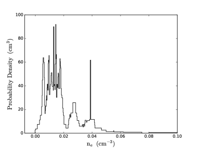
Figure 11.— Probability density function for the mean electron density calculated as $n_{\rm e}={\rm DM}\times{\rm parallax(mas})/1000$. Errors on parallaxes are included by representing the contribution from each pulsar as a rectangle function centered on the nominal value and width equal to the sum of the positive and negative-going errors. The three objects with lower limits on their distances are also included. The PDF is normalized to unit area.

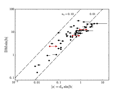
Figure 12.— Plot of the $z$ component of DM vs. distance $z$ from the Galactic plane for the data. The dashed lines show the variation expected for constant values of electron density, $0.01$ cm^-3 and $0.1$ cm^-3. The arrows denote objects with lower bounds on their distances, J1650$-$1654, J2150+5247, and J2325+6316.

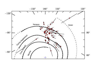
Figure 13.—  pulsars projected onto the Galactic plane using parallax distances and their errors. Objects with lower bounds on their distances and objects with greater than a 5:1 distance ratio (maximum to minimum parallax distance) are excluded. The spiral arms and their labels are identical to those used in the NE2001 model.

Figure 12 shows the perpendicular component ${\rm DM}_{z}={\rm DM}\sin|b|$ plotted against the $z$ distance of each pulsar from the Galactic plane. Dashed lines show the expected values for constant densities of $0.01$ and $0.1$ cm^-3. Most of the points are between these two lines except at large values of $z$, where there appears to be a maximum in ${\rm DM}_{z}$ even though about eight of the  pulsars extend from two to five kpc above the plane. The  sample by itself therefore verifies that the Galaxy must have an electron density component similar to the thick disk component in the NE2001 (Cordes & Lazio, 2002) and YMW16 (Yao et al., 2017) models.

Distances of  pulsars projected onto the Galactic plane (Fig. 13) show that the sample extends to large distances parallel to the plane and sample several spiral arms (as defined in the NE2001 model).

Galactic electron density models are based on a wide variety of measurements but ultimately require independently obtained distances for as many pulsars as possible. The NE2001 model used distance constraints on 112 pulsars of which only 14 were parallax measurements; the remainder were mostly from HI-absorption constrained distances and from pulsars in globular clusters. For the YMW16 model, 73 parallax measurements were used, many from pulsar timing, but 29% had a constrained distance range (maximum to minimum ratio) of 1.5:1 and 13% had more than a 2:1 range.

The performance of the NE2001 and YMW16 models can be compared against the  distances as a ‘blind’ test because the  sample was not used in the construction of either model. The comparison is particularly useful for more distant pulsars; the median distance of the  sample is 2.5 kpc, while the median distance to pulsars with previously published VLBI parallaxes is 1.1 kpc.

Figure 14 shows the ratio $d_{\pi}/d_{\rm model}$ for the NE2001 and YMW16 models in the top and bottom panels respectively. Circle sizes indicate values of this ratio while colors indicate approximate distances. Comparison of the two figures indicates that both models show large errors for some objects, with the NE2001 model doing better on some objects, and the YMW16 model on others. The YMW16 model performs somewhat better on a few high-latitude pulsars than the NE2001 model. The distances of two pulsars with the most negative latitudes (the red circles between 60^∘ and 90^∘ longitude) are overestimated in the YMW16 model and underestimated by the NE2001 model. The median distance ratio exceeds unity for both models (1.5 and 1.1 for NE2001 and YMW16, respectively) and the RMS values of this ratio are 1.1 and 0.8, respectively. These results demonstrate that the new  sample will be extremely valuable for the next generation Galactic electron density distribution model.

Yao et al. (2017) claim that in 95% of cases, the YMW16 predicted distance $d_{\mathrm{YMW}}$ will fall within the range $\left(0.1\times d_{\mathrm{actual}},1.9\times d_{\mathrm{actual}}\right)$. This claim can be examined using the  dataset. We restrict ourselves to pulsars whose VLBI parallax significance is at least 5$\sigma$, of which there are 42. Of these 42 pulsars, six have a predicted YMW16 distance that falls outside the range $\left(0.1\times d_{\pi_{\mathrm{min}}},1.9\times d_{\pi_{\mathrm{max}}}\right)$, where $d_{\pi_{\mathrm{min}}}$ and $d_{\pi_{\mathrm{max}}}$ are the values given by inverting the 95% confidence interval for parallax. This would be inconsistent with 95% of the YMW16 distances falling within the range $\left(0.1\times d_{\mathrm{actual}},1.9\times d_{\mathrm{actual}}\right)$, if the  sample was representative of the entire pulsar population. However, the  sample is explicitly not an unbiased sample of pulsars, and in particular pulsars at high Galactic latitudes are intentionally over-represented in order to help constrain the Galactic scale height. Of the six discrepant YMW16 predictions, five are at moderate to high Galactic latitudes ($|b|>20$^∘ and the YMW16 model places them beyond the edge of the Galaxy, while the median Galactic latitude of the 42 pulsars with a significant parallax distance is 14^∘. The sixth source, at $b=11.3$^∘, is underpredicted by an order of magnitude. Accordingly, based on the  sample we advise that all DM–based distance estimates be used with caution, especially for high Galactic latitude pulsars.

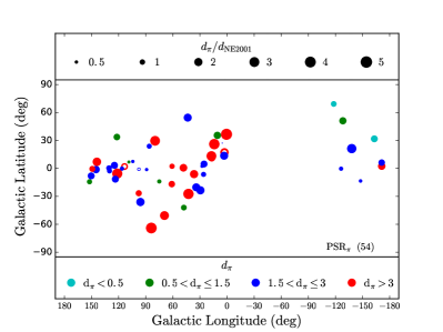
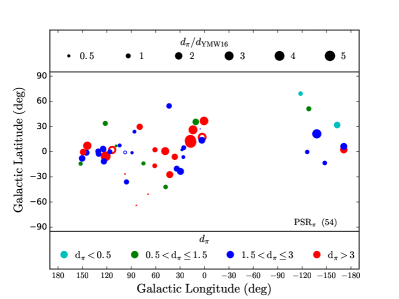
Figure 14.— Ratio of VLBI parallax distance to the NE2001 model distance (top panel) and the YMW16 model distance (bottom panel). The results are shown as a function of Galactic longitude and latitude. Circle sizes indicate the value of the ratio, as shown in the upper legend in each panel. Circle colors denote parallax distance in kpc as in the lower legend in each panel. Filled circles denote distance measurements while the three open circles indicate lower bounds on pulsar distances.

Finally, as noted in Section 3.2, refractive wander is potentially a significant contributor to the differential astrometry error budget for some lines of sight, particularly at low Galactic latitude. While beyond the scope of this work, future analysis using the  sample could refine the scattering disk and refractive wander predictions of the NE2001 model, leading to improved estimates of systematic error contributions for future studies.

4.3. Transverse velocities

Galactic pulsars have a larger scale height than their progenitor massive stars, leading to the early inference that they have high velocities (Gunn & Ostriker, 1970). Individual high velocity objects such as PSR B1508+55 ($v_{\perp}\sim 1000$ km s^-1; Chatterjee et al., 2005) and PSR J2225+6535, the Guitar Nebula pulsar ($v_{\perp}\sim 800$ km s^-1; this work; Cordes et al., 1993) establish stringent constraints on natal kicks and the minimum asymmetry requirements in simulations of supernova core collapse (e.g., Fryer, 2004), and the overall population velocities inform models for neutron star birth, supernova explosions, and the evolution of close binary systems. The pulsar velocity distribution has therefore been a topic of continued interest (e.g. Lyne & Lorimer, 1994; Hansen & Phinney, 1997; Cordes & Chernoff, 1998; Arzoumanian et al., 2002; Hobbs et al., 2005; Verbunt et al., 2017).

The parallax and proper motion measurements presented here provide model-independent estimates of pulsar distances and transverse velocities (Table LABEL:tab:derivedresults) and thus mitigate a key uncertainty in deriving the pulsar velocity distribution. We note, however, that the astrophysically relevant quantity is the 3-dimensional birth velocity for the entire pulsar population. For individual pulsars, their uncertain age limits the precision of any extrapolation in the Galactic gravitational potential, and their radial velocity is unknown, rendering a full 3-dimensional birth velocity unmeasurable. While such uncertainties can be addressed statistically, the inference of population parameters is further affected by biases in the sample of objects with precise astrometry (see, e.g., Arzoumanian et al., 2002). The targets in this work were selected based on flux density and calibrator availability (Section 2.1), and inferring the properties of the population would require the addressing of selection effects in the original detection surveys. Such selection effects are not trivial: for example, many pulsar surveys focus on the Galactic plane where the stellar progenitors of pulsars are concentrated, but on average, the higher velocity neutron stars will spend less time near the Galactic plane compared to the lower velocity objects. Thus the high velocity tail of the pulsar population will be suppressed in a typical survey yield.

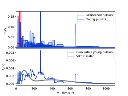
Figure 15.— The transverse velocity distribution of the PSR$\pi$ sample of pulsars. Top: Histograms of the measured velocities ($\pm 1\sigma$) of the young (blue) and millisecond (recycled; red) pulsars, as listed in Table LABEL:tab:derivedresults. Bottom: The transverse velocity probability distribution, summed across all young pulsars in our sample, with a model for the pulsar velocity distribution from Verbunt et al. (2017) scaled to two dimensions and overlaid for comparison.

We defer the treatment of the full range of selection effects to future work, but here we present histograms of the measured transverse velocities for each pulsar in our sample, along with a normalised probability distribution summing across all pulsars (Figure 15). Note that the four millisecond (recycled) pulsars in our sample, PSRs J1022$+$1001, J2010$-$1323, J2145$-$0750, and J2317$+$1439, are excluded from the cumulative distribution, since recycled pulsars are an older population with a lower characteristic velocity distribution (e.g., Cordes & Chernoff, 1997). As a comparison for our sample of transverse velocities, we plot a recent velocity distribution model for young pulsars (Verbunt et al., 2017), scaled to two dimensions. The distribution of transverse velocities of the sample of young pulsars presented here is broadly compatible with previous published models, and a detailed treatment of selection effects is required before the models can be usefully discriminated between.

As an aside, we note that the present work provides the first model-independent distance and velocity estimate for PSR J2225+6535, the Guitar Nebula pulsar ($v_{\perp}\sim 800$ km s^-1; Table LABEL:tab:derivedresults). That is the highest well-measured velocity in the current sample, although somewhat lower than previous estimates (e.g., Chatterjee & Cordes, 2004); further analysis and comparison to long-term optical monitoring of the time-evolution of the H$\alpha$ bow shock nebula is underway.

4.4. Comparison to timing astrometry

As highlighted in Section 1, having independent measurements of pulsar distances and astrometric parameters is extremely valuable for several pulsar science cases. While pulsar timing can provide the pulsar DM, extracting a distance from this measurement is dependent on having an accurate model of the Galactic electron density (see Section 4.2). Moreover, multi-frequency (or wide-band) observations are required to obtain a good DM measurement.

Astrometric terms in pulsar timing models are covariant with red noise in timing data that arises from fluctuations in the pulsar spin-down and/or propagation delays through the ISM that are not completely captured in the pulsar ephemeris. As shown in Deller et al. (2016) and Madison et al. (2013), red noise can lead to substantial errors in the values and underestimates of the uncertainty for timing-derived parameters. These errors are especially large for unrecycled pulsars with surface field strengths $\sim 10^{11}$ - $10^{13}$ G, but are present at some level for all pulsars.

The highest precision measurements from pulsar timing are obtained with millisecond pulsars (MSPs) due to their frequent, short pulses and stable rotation. In our sample we have four MSPs: PSR J1022$+$1001, PSR J2010$-$1323, PSR J2145$-$0750, and PSR J2317$+$1439. The VLBI results for PSR J1022$+$1001 and PSR J2145$-$0750 were already presented and discussed in Deller et al. (2016) and compared with the most recent pulsar timing measurements. For completeness, we summarize the results here for all MSPs in the  sample. Each of these pulsars is observed by at least one pulsar timing array (PTA) in the search for low-frequency gravitational waves (e.g., Verbiest et al., 2016).

PSR J1022$+$1001 is located extemely close to the ecliptic plane (ecliptic latitude $\beta$=-0.06^∘) , which in pulsar timing leads to suboptimal measurements of the position and proper motion, due to the components being covariant in equatorial coordinates. Moreover, low-ecliptic latitude pulsars have their line-of-sight passing close to the Sun every year which leads to annual increases of DM which may not be modelled optimally in pulsar timing (e.g. Tiburzi & Verbiest, 2018).

Although PSR J2010$-$1323 is also located relatively close to the ecliptic plane ($\beta$=6.49^∘), pulsar timing has been able to measure the proper motion of this pulsar with relatively high accuracy, as shown in Table 7. This pulsar is observed by the European Pulsar Timing Array (EPTA) and the North American Nanohertz Observatory for Gravitational Waves (NANOGrav), but not the Parkes Pulsar Timing Array (PPTA). Figure 16 shows that the uncertainties from their timing programmes are comparable to VLBI, and no significant discrepancies are seen. It is noteworthy that the 11-yr NANOGrav dataset values (Arzoumanian et al., 2018) changed significantly from the 9-yr values (Matthews et al., 2016), which were inconsistent at the $\gtrsim$2$\sigma$ level with the VLBI and EPTA values (Desvignes et al., 2016).

PSR J2145$-$0750 is observed by all three PTAs, and is a good example where VLBI measurements give up to an order-of-magnitude improved accuracy compared to some timing measurements. The ecliptic latitude of this pulsar is 5.31 degrees, and this pulsar is known to show DM variations that affect the timing observations (e.g. Arzoumanian et al., 2018). As was the case for PSR J2010-1323, the proper motion obtained for PSR J2145$-$0750 from the NANOGrav 11-yr dataset is considerably less discrepant with other measurements (our VLBI results, and also the PPTA and EPTA timing results) than the proper motion from the NANOGrav 9-yr dataset was.

As described in Section 4.1, the VLBI astrometry of PSR J2317$+$1439 resulted in relatively poor constraints due to failed observations, which all fell on the same side of the parallax extrema. This also resulted in very conservative and skewed uncertainties for the proper motion parameters when using the bootstrapping method (green error ellipse in Figure 16), and all timing-derived measurement are consistent with the VLBI values. When using the least-squares fitting method, the uncertainties are reduced (black curve in Figure 16), and the EPTA timing value is offset by about $1\sigma$ from the VLBI value. Additional observations for PSR J2317$+$1439 could greatly reduce the VLBI proper motion uncertainty and provide a much more stringest comparison against timing.

Overall, Figure 16 shows that although for MSPs in some cases the timing measurements of proper motion parameters are comparable to the accuracy of VLBI measurements, the actual values can differ significantly between PTAs. As discussed in Deller et al. (2016), there could be multiple explanations, such as contamination by annual DM variations, systematic instrumental noise, the use of different versions of Solar System ephemeris (SSE), or including different levels of noise modelling in the timing solutions. Arzoumanian et al. (2018) find the effect of using a different SSE on the proper motion to be on the order of 10 $\mu\mathrm{as}$ yr^-1 or less, which is insignificant compared to the current uncertainty levels.

Besides further comparison between timing models and e.g. the effect of including different types of noise modelling and DM correction, an extended set of independent and improved VLBI measurements of MSP proper motions will be extremely useful to find the underlying causes of any discrepancies between measured values.

Table 8 shows that in order to derive an independent distance measurement, VLBI observations can play an essential role to improve pulsar timing. In general, measuring a parallax signature in pulsar timing data is dependent on having a long baseline of observations, and as seen in Table 8 the uncertainties are between a factor of 2 and an order of magnitude larger compared to what is achieved with VLBI within 2 years.

Finally, a comparison was made between the proper motions of the non-MSPs in our sample and the proper motions derived from timing observations. However, none of these pulsars had sufficiently significant detections from timing (Hobbs et al., 2004; Zou et al., 2005; Li et al., 2016) to make a useful comparison with our VLBI-derived values. When compared to previously derived interferometric measurements (see Table 9) we find that al most all are consistent within the given (generally low precision) error bounds; the exceptions are PSR B0329+54 and PSR B1133+16, for which the previous VLBI proper motion measurements of Brisken et al. (2002) are discrepant at the $\gtrsim$2$\sigma$ level in the declination coordinate.

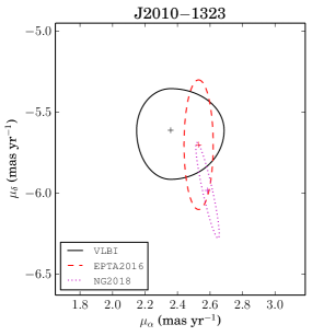
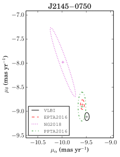
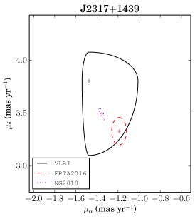
Figure 16.— Comparison of proper motion measurements from VLBI and different PTA programmes. References: EPTA: Desvignes et al. (2016); NANOGrav: Arzoumanian et al. (2018); PPTA: Reardon et al. (2016).

Table 7Comparison between proper motion measurements

Pulsar	VLBI	EPTA	NANOGrav	PPTA
J1022$-$1001 $\mu_{\alpha}$	-14.92${}^{+0.05}_{-0.03}$	-18.2(64)	–	-17.09(3)
J1022$-$1001 $\mu_{\delta}$	5.61${}^{+0.03}_{-0.04}$	-3(16)	–	–
J2010$-$1323 $\mu_{\alpha}$	2.36${}^{+0.33}_{-0.21}$	2.53(9)	2.59(5)	–
J2010$-$1323 $\mu_{\delta}$	-5.61${}^{+0.26}_{-0.30}$	-5.7(4)	-6.0(2)	–
J2145$-$0750 $\mu_{\alpha}$	-9.49${}^{+0.05}_{-0.04}$	-9.58(4)	-10.0(2)	-9.59(8)
J2145$-$0750 $\mu_{\delta}$	-9.11${}^{+0.09}_{-0.08}$	-8.86(10)	-8.0(5)	-8.9(3)
J2317$+$1439 $\mu_{\alpha}$	-1.43${}^{+0.08}_{-0.08}$	-1.19(7)	-1.36(2)	–
J2317$+$1439 $\mu_{\delta}$	3.74${}^{+0.18}_{-0.18}$	3.33(13)	3.49(4)	–

Table 8Comparison between parallax measurements

Pulsar	VLBI	EPTA	NANOGrav	PPTA
J1022$-$1001	1.39${}^{+0.04}_{-0.03}$	0.72(20)	–	1.1(3)
J2010$-$1323	0.48${}^{+0.17}_{-0.12}$	–	0.3(1)	–
J2145$-$0750	1.60${}^{+0.06}_{-0.01}$	1.53(11)	1.6(4)	1.84(17)
J2317$+$1439	0.65${}^{+0.07}_{-0.07}$	0.7(3)	0.50(8)	–

Table 9Previous interferometric proper motion measurements of normal pulsars from the literature

Pulsar name (B1950)	Pulsar name (J2000)	PMRA (mas yr-1)	PMDEC (mas yr-1)	Reference
B0148-06	J0151-0635	15(47)	-30(34)	Harrison et al. (1993)
B0149-16	J0152-1637	3.1(12)	-27(2)	Brisken et al. (2003)
B0320+39	J0323+3944	16(6)	-30(5)	Harrison et al. (1993)
B0329+54	J0332+5434	17.0(3)	-9.5(4)	Brisken et al. (2002)
B0559-05	J0601-0527	18(8)	-16(7)	Harrison et al. (1993)
B0611+22	J0614+2229	-4(5)	-3(7)	Harrison et al. (1993)
B0626+24	J0629+2415	-7(12)	2(12)	Harrison et al. (1993)
B0823+26	J0826+2637	62.6(24)	95.3(24)	Gwinn et al. (1986)
B1133+16	J1136+1551	-74.0(4)	368.1(3)	Brisken et al. (2002)
B1322+83	J1321+8323	-53(20)	13(7)	Harrison et al. (1993)
B1540-06	J1543-0620	-17(2)	-4(3)	Brisken et al. (2003)
B1604-00	J1607-0032	-1(14)	-7(9)	Lyne et al. (1982)
B1642-03	J1645-0317	-3.7(15)	30.0(16)	Brisken et al. (2003)
B1732-07	J1735-0724	-2.4(17)	28(3)	Brisken et al. (2003)
B1839+56	J1840+5640	-30(4)	-21(2)	Harrison et al. (1993)
B1917+00	J1919+0021	-2(30)	-1(10)	Harrison et al. (1993)
B2044+15	J2046+1540	-13(6)	3(4)	Harrison et al. (1993)
B2110+27	J2113+2754	-23(2)	-54(3)	Harrison et al. (1993)
B2148+63	J2149+6329	14(3)	10(4)	Harrison et al. (1993)
B2224+65	J2225+6535	144(3)	112(3)	Harrison et al. (1993)
B2303+30	J2305+3100	2(2)	-20(2)	Brisken et al. (2003)
B2351+61	J2354+6155	22(3)	6(2)	Harrison et al. (1993)
B0820+02	J0823+0159	5(11)	-1(8)	Harrison et al. (1993)
B0823+26	J0826+2637	61(3)	-90(2)	Lyne et al. (1982)
B2043-04	J2046-0421	9(16)	-7(8)	Harrison et al. (1993)

4.5. Absolute positional accuracy

Three factors contribute to the accuracy of pulsar absolute positions that we can obtain from phase-referenced VLBI observations:

1. the accuracy of the off-beam calibrator absolute position;

2. a contribution from the frequency-dependent core-shift of the off-beam calibrator; and

3. the accuracy of the determination of position offsets with respect to the off-beam calibrators.

We now consider each of these effects in turn for the  sample.

Among 60 sources used as off-beam calibrators, the absolute position accuracy (as recorded in the Radio Fundamental Catalog; http://astrogeo.org/rfc/) ranged from 0.10 to 0.37 mas, with a median of 0.17 mas.

We have not measured the core-shift of any of the off-beam calibrators in our observations. Therefore, we can present only a rough estimate of its unaccounted contribution. Sokolovsky et al. (2011) presented results of multifrequency observations of core-shift. The core-shift of 17 AGNs at 1.6 GHz varied from 0.4 to 2.2 mas with the median 1.1 mas. We can take this estimate and assume it is typical for the sources used by the  sample.

According to Table LABEL:tab:allresults, uncertainties in the position offsets from the pulsars to their position reference source range from 0.04 to 1.1 mas, with a median of 0.09 mas. The offset from the position reference source to the out-of-beam calibrator is typically be an order of magnitude greater, given the typical angular separations (14′ median separation from position reference to target, vs 1.9^∘ for off-beam calibrator to target).

Assuming these sources of errors to be independent, the overall uncertainties in the  pulsar absolute positions range from 0.4 to $\sim$10 mas, with a median of 1.4 mas (Table LABEL:tab:derivedresults). The unaccounted core-shift in the off-beam calibrator and the position offset from the off-beam calibrator to the position reference source contribute roughly equally in most cases, and generally dominate over the absolute position uncertainty of the off-beam calibrator.

The absolute pulsar position does not play a significant role in the context of our study, but this does not mean it is not valuable at all. Comparison of the VLBI pulsar positions with positions determined with pulsar timing provides important information. First, a determination of the net rotation of pulsar positions determined with timing against the positions determined with VLBI can be used to improve three parameters that describe the orientation of the Earth orbit in the inertial space, i.e., the position of the ecliptic pole and the point of vernal equinox. Second, analysis of the residual position differences between timing and VLBI after the removal of net rotation gives us a measure of possible systematic errors in VLBI and/or timing. Timing and VLBI position estimates are to a great extent independent, and therefore, their intercomparson provides us a unique opportunity to make an assessment of their accuracy.

Dedicated VLBA observations are able to bring the absolute accuracy of calibrator positions down to at least 0.1 mas. As Fey et al. (2015) demonstrated via decimation tests, a level of 0.05 mas for random position errors can even be reached if sources are observed long enough. Reaching that level of accuracy requires additional observations in the mode of absolute astrometry, similar to the regular geodesy “RDV” program conducted on the VLBA (Petrov et al., 2009).

The most important step for improvement of accuracy of pulsar VLBI absolute astrometry is determination of the core-shift. This requires multi-frequency dedicated observations and analysis, which we have not utilised for . Sokolovsky et al. (2011) describes the technique of such observations. As it was shown in this and following works, frequency dependence of observed core-shifts obeys the power law $\nu^{-1/r}$, with $r$ close to 1. It was shown theoretically by Lobanov (1998) that in a case if i) the plasma is in the state of equipartition with the magnetic field, ii) the dominating absorption mechanism is synchrotron self-absorption, and iii) the jet has a conical shape, then $r=1$.

Determination of the core-shift requires significant observational resources and it is not practical to do it for every pulsar. The  program is presently being continued with a second sample consisting exclusively of millisecond pulsars: $\mathrm{MSPSR}\pi$, with observations of 18 millisecond pulsars taking place during the period 2015 – 2018 and first results reported in Vigeland et al. (2018). To facilitate a comparison between high-precision pulsar timing and VLBI absolute positions, we have decided to focus on a list of 17 millisecond pulsars drawn from  and $\mathrm{MSPSR}\pi$ that have timing positions accurate to 1 mas or better. In March 2018 we commenced a VLBA program targeting their off-beam calibrators, aiming to improve the absolute positions of these sources to the 0.1 mas level, as well as measuring the core-shift at 1.6 GHz. As of August 2018, 28% of planned observations have been conducted.

For pulsars in binary systems, an optically-visible companion offers the possibility of comparing VLBI positions against Gaia positions for truly point-like sources, avoiding the problems of systematic VLBI–Gaia offsets that are located preferentially along the jet direction of AGN (Kovalev et al., 2017). Unfortunately, pulsars with bright optical companions are rare; of the four binary pulsars in , none have a companion above the Gaia magnitude limit. Given that over 9,000 common sources can be identified in VLBI and Gaia catalogs (Petrov et al., 2019), the sheer weight of numbers means that an ensemble comparison of radio/optical AGN will provide a more accurate alignment of VLBI and Gaia positions than will be possible with pulsar companions.

4.6. Achievable accuracy of differential VLBI pulsar astrometry

As discussed in Section 3.2, the astrometric accuracy achieved for a given target is expected to be influenced by the target brightness, the calibrator brightness, the target–calibrator separation, and the average observing conditions (principally the magnitude of the ionospheric gradients and the observing elevation). In Figures 17 – 19, we explore this hypothesis by examining the parallax uncertainty achieved for  pulsars as a function of each potential influence separately, before attempting to find an parameterized function that predicts the achieved accuracy given the known observing parameters. In all plots, we have excised PSR J2317+1439, where the parallax uncertainty is artificially inflated by the non-detections of the pulsar discussed in Section 4.1.5, and the red line shows a best-fit linear regression. The parallax uncertainty shown is the width of the 68% confidence interval in milliarcseconds (i.e., the addition of the uncertainties in the positive and negative directions).

Figure 17 shows the parallax uncertainty plotted against the average signal–to–noise ratio (S/N) achieved on the target. Because the brightest pulsars achieve very high S/N, a log scale is used for the x-axis. As expected, the faintest targets tend to have higher uncertainties, but systematic errors dominate in most cases.

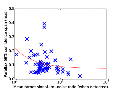
Figure 17.— Parallax uncertainty for  pulsars plotted against the average signal–to–noise ratio achieved on the target (disregarding non–detections, if there were any). The red line shows a best-fit linear regression.

Figure 18 shows the parallax uncertainty plotted against separation to the position reference source. A weak trend towards larger uncertainties at larger separations is seen, but with a large scatter ($r^{2}=0.08$, where $r$ is the correlation coefficient).

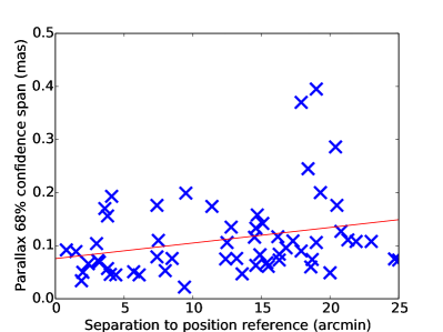
Figure 18.— Parallax uncertainty for  pulsars plotted against angular separation to the in–beam position reference source. The red line shows a best-fit linear regression.

Figure 19 shows the parallax uncertainty plotted against the average S/N achieved on the inbeam calibrator, or the quadrature addition of the S/N if multiple calibrators were used. Because the brightest calibrators achieve very high S/N, a log scale is used for the x-axis. The pulsars with the faintest calibrators tend to have higher uncertainties, but calibrator brightness is no more dominant than calibrator–target separation.

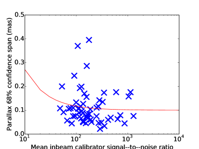
Figure 19.— Parallax uncertainty for  pulsars plotted against the average signal–to–noise ratio achieved on the inbeam calibrator source(s). The red line shows a best-fit linear regression.

Finally, we use a multiparameter estimation including calibrator S/N, elevation–weighted calibrator–target separation, and target S/N to attempt to predict the parallax accuracy achieved in a  observing setup. The predicted parallax error $\pi_{\mathrm{p}}$ in mas is given by:

$$\pi_{\mathrm{p}}=\sqrt{\left(\frac{A}{\mathrm{S/N}_{t}\times\sqrt{N_{\mathrm{obs}}}}\right)^{2}+\ \left(\frac{B}{\mathrm{S/N}_{c}}\right)^{2}+\left(C\times\Delta\theta\right)^{2}}$$ (2)

where $A$, $B$, and $C$ are constants which we fit from our dataset and find values $A=9.0$, $B=4.5$, $C=0.0028$, $\mathrm{S/N}_{t}$ is the average signal–to–noise ratio on the target, $N_{\mathrm{obs}}$ is the number of observations, $\mathrm{S/N}_{c}$ is the average signal–to–noise ratio on the in–beam calibrator, and $\Delta\theta$ is the angular separation of the pulsar and in-beam calibrator in arcminutes divided by the sine of the average observing elevation.

Figure 20 shows the actual parallax uncertainty $\pi_{\mathrm{obs}}$ vs the predicted value given by Equation 2, with the red line highlighting the expected 1:1 relationship. Over 80% of the pulsars fall within the range $0.5\times\pi_{\mathrm{p}}<\pi_{\mathrm{obs}}<2\times\pi_{\mathrm{p}}$, indicated by the grey lines on the plot.

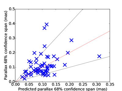
Figure 20.— Parallax uncertainty for  pulsars plotted against the predicted parallax uncertainty based on calibrator S/N, target S/N, and calibrator–target separation given in Equation 2. The red line shows a 1:1 relationship, while the grey lines show $\pi_{\mathrm{obs}}=0.5\times\pi_{\mathrm{p}}$ and $\pi_{\mathrm{obs}}=2\times\pi_{\mathrm{p}}$.

The values of the constants fitted in Equation 2 can be used with caution to estimate the probable astrometric accuracy of a future 1600 MHz VLBA astrometric campaign of comparable duration (8 epochs). For instance, in the limit of a very bright target and calibrator, then for an observation with typical observing elevation of 45^∘, the expected parallax uncertainty is 4 $\mu$as per arcminute of separation to the in-beam calibrator. Alternatively, given a target accuracy, these results can be used to estimate the characteristics of the in-beam calibrator that will be required. For a bright target, if the desired parallax accuracy is 20 $\mu$as, the in-beam calibrator should be separated by no more than 5 arcminutes from the target, and should be at least $\sim$20 mJy (in order to achive the necessary signal–to–noise ratio of 225). Obviously, extending the number of observations in the campaign could be undertaken to lower these expected limits.

5. Conclusions

We have presented the largest sample of VLBI astrometric results for radio pulsars assembled to date, obtaining a significant ($>$2$\sigma$) parallax for 53 pulsars using the VLBA. Under moderately unfavourable observing conditions (relatively close to solar maxima, where ionospheric disturbances are more prevalent), we obtain a median parallax accuracy of $\sim$40 $\mu$as, meaning that precise distances can be obtained for pulsars out to $\sim$2.5 kpc, and reasonable constraints a factor of 2–3 further. Observations with the VLBA at higher sensitivity (the standard continuum recording rate is now 4 times higher, doubling the sensitivity of comparable observations) and in more favourable ionospheric conditions should be capable of measuring a parallax-based distance for almost any sufficiently bright pulsar in the northern sky.

Comparisons of  distances to those predicted by the NE2001 and YMW16 Galactic electron density distribution models show that distance predictions based on dispersion measure are less accurate than claimed, although the biased nature of the  sample makes it difficult to quantify the level at which the DM–based distance uncertainties are typically underestimated. It is clear, however, that results for nearby pulsars and pulsars at high Galactic latitudes should be treated with particular caution.

Extending the comparison of pulsar timing astrometry to VLBI with two additional new pulsars, we reinforce that timing proper astrometry can yield underestimated errors, particularly for pulsars at low ecliptic latitude.

Finally, we use the ensemble of  results to estimate the typical astrometric accuracy that could be obtained at 1600 MHz with the VLBA, where a suitable in-beam calibrator can almost always be found in regions where Galactic scattering is not too intense. For a typical astrometric program like  with 8 observing epochs spread over 18 months and clustered near the parallax extrema, the parallax accuracy attainable in the limit of a sufficiently bright target and a brighth and stable calibrator is around 4 $\mu\mathrm{as}$ per arcminute of separation. Since the typical calibrator–target separation is of order 10 arcminutes, this implies that high quality parallax distances can be obtained at 1600 MHz out to several kpc. With a smaller calibrator–target separation (either through good fortune, or higher sensitivity enabling the use of weaker calibrators), precise distances can be obtained up to $\sim$10 kpc.

References

- Abdo et al. (2013) Abdo, A. A., Ajello, M., Allafort, A., et al. 2013, ApJS, 208, 17
- Arzoumanian et al. (2002) Arzoumanian, Z., Chernoff, D. F., & Cordes, J. M. 2002, ApJ, 568, 289
- Arzoumanian et al. (2018) Arzoumanian, Z., Brazier, A., Burke-Spolaor, S., et al. 2018, ApJS, 235, 37
- Becker et al. (1995) Becker, R. H., White, R. L., & Helfand, D. J. 1995, ApJ, 450, 559
- Brisken et al. (2002) Brisken, W. F., Benson, J. M., Goss, W. M., & Thorsett, S. E. 2002, ApJ, 571, 906
- Brisken et al. (2003) Brisken, W. F., Fruchter, A. S., Goss, W. M., Herrnstein, R. M., & Thorsett, S. E. 2003, ApJ, 126, 3090
- Caraveo et al. (2001) Caraveo, P. A., De Luca, A., Mignani, R. P., & Bignami, G. F. 2001, ApJ, 561, 930
- Chatterjee & Cordes (2004) Chatterjee, S., & Cordes, J. M. 2004, ApJ, 600, L51
- Chatterjee et al. (2005) Chatterjee, S., Vlemmings, W. H. T., Brisken, W. F., et al. 2005, ApJ, 630, L61
- Chatterjee et al. (2009) Chatterjee, S., Brisken, W. F., Vlemmings, W. H. T., et al. 2009, ApJ, 698, 250
- Condon (1997) Condon, J. J. 1997, PASP, 109, 166
- Condon et al. (1998) Condon, J. J., Cotton, W. D., Greisen, E. W., et al. 1998, AJ, 115, 1693
- Cordes & Chernoff (1997) Cordes, J. M., & Chernoff, D. F. 1997, ApJ, 482, 971
- Cordes & Chernoff (1998) —. 1998, ApJ, 505, 315
- Cordes & Lazio (2002) Cordes, J. M., & Lazio, T. J. W. 2002, ArXiv e-prints, 0207156, astro-ph/0207156
- Cordes et al. (1993) Cordes, J. M., Romani, R. W., & Lundgren, S. C. 1993, Nature, 362, 133
- Deller et al. (2013) Deller, A. T., Boyles, J., Lorimer, D. R., et al. 2013, ApJ, 770, 145
- Deller & Middelberg (2014) Deller, A. T., & Middelberg, E. 2014, AJ, 147, 14
- Deller et al. (2009) Deller, A. T., Tingay, S. J., Bailes, M., & Reynolds, J. E. 2009, ApJ, 701, 1243
- Deller et al. (2007) Deller, A. T., Tingay, S. J., Bailes, M., & West, C. 2007, PASP, 119, 318
- Deller et al. (2011) Deller, A. T., Brisken, W. F., Phillips, C. J., et al. 2011, PASP, 123, 275
- Deller et al. (2012) Deller, A. T., Archibald, A. M., Brisken, W. F., et al. 2012, ApJ, 756, L25
- Deller et al. (2016) Deller, A. T., Vigeland, S. J., Kaplan, D. L., et al. 2016, ApJ, 828, 8
- Demorest et al. (2010) Demorest, P. B., Pennucci, T., Ransom, S. M., Roberts, M. S. E., & Hessels, J. W. T. 2010, Nature, 467, 1081
- Desvignes et al. (2016) Desvignes, G., Caballero, R. N., Lentati, L., et al. 2016, MNRAS, 458, 3341
- Efron & Tibshirani (1991) Efron, B., & Tibshirani, R. 1991, Science, 253, 390
- Fey et al. (2015) Fey, A. L., Gordon, D., Jacobs, C. S., et al. 2015, AJ, 150, 58
- Fryer (2004) Fryer, C. L. 2004, ApJ, 601, L175
- Greisen (2003) Greisen, E. W. 2003, Information Handling in Astronomy - Historical Vistas, 285, 109
- Guélin et al. (1969) Guélin, M., Guibert, J., Huchtmeier, W., & Weliachew, L. 1969, Nature, 221, 249
- Gunn & Ostriker (1970) Gunn, J. E., & Ostriker, J. P. 1970, ApJ, 160, 979
- Gwinn et al. (1986) Gwinn, C. R., Taylor, J. H., Weisberg, J. M., & Rawley, L. A. 1986, AJ, 91, 338
- Hansen & Phinney (1997) Hansen, B. M. S., & Phinney, E. S. 1997, MNRAS, 291, 569
- Harrison et al. (1993) Harrison, P. A., Lyne, A. G., & Anderson, B. 1993, MNRAS, 261, 113
- Hobbs et al. (2005) Hobbs, G., Lorimer, D. R., Lyne, A. G., & Kramer, M. 2005, MNRAS, 360, 974
- Hobbs et al. (2004) Hobbs, G., Lyne, A. G., Kramer, M., Martin, C. E., & Jordan, C. 2004, MNRAS, 353, 1311
- Igoshev et al. (2016) Igoshev, A., Verbunt, F., & Cator, E. 2016, A&A, 591, A123
- Kettenis et al. (2006) Kettenis, M., van Langevelde, H. J., Reynolds, C., & Cotton, B. 2006, in Astronomical Society of the Pacific Conference Series, Vol. 351, Astronomical Data Analysis Software and Systems XV, ed. C. Gabriel, C. Arviset, D. Ponz, & S. Enrique, 497
- Kovalev et al. (2008) Kovalev, Y. Y., Lobanov, A. P., Pushkarev, A. B., & Zensus, J. A. 2008, A&A, 483, 759
- Kovalev et al. (2017) Kovalev, Y. Y., Petrov, L., & Plavin, A. V. 2017, A&A, 598, L1
- Larchenkova et al. (2017) Larchenkova, T. I., Lutovinov, A. A., & Lyskova, N. S. 2017, ApJ, 835, 51
- Li et al. (2016) Li, L., Wang, N., Yuan, J. P., et al. 2016, MNRAS, 460, 4011
- Lobanov (1998) Lobanov, A. P. 1998, A&A, 330, 79
- Lyne et al. (1982) Lyne, A. G., Anderson, B., & Salter, M. J. 1982, MNRAS, 201, 503
- Lyne & Lorimer (1994) Lyne, A. G., & Lorimer, D. R. 1994, Nature, 369, 127
- Madison et al. (2013) Madison, D. R., Chatterjee, S., & Cordes, J. M. 2013, ApJ, 777, 104
- Marcaide & Shapiro (1984) Marcaide, J. M., & Shapiro, I. I. 1984, ApJ, 276, 56
- Matthews et al. (2016) Matthews, A. M., Nice, D. J., Fonseca, E., et al. 2016, ApJ, 818, 92
- Middelberg et al. (2013) Middelberg, E., Deller, A. T., Norris, R. P., et al. 2013, A&A, 551, A97
- Minter et al. (2008) Minter, A. H., Camilo, F., Ransom, S. M., Halpern, J. P., & Zimmerman, N. 2008, ApJ, 676, 1189
- Moór et al. (2011) Moór, A., Frey, S., Lambert, S. B., Titov, O. A., & Bakos, J. 2011, AJ, 141, 178
- O’Sullivan & Gabuzda (2009) O’Sullivan, S. P., & Gabuzda, D. C. 2009, MNRAS, 400, 26
- Petrov et al. (2009) Petrov, L., Gordon, D., Gipson, J., et al. 2009, Journal of Geodesy, 83, 859
- Petrov et al. (2019) Petrov, L., Kovalev, Y. Y., & Plavin, A. V. 2019, MNRAS, 482, 3023
- Plavin et al. (2019) Plavin, A. V., Kovalev, Y. Y., Pushkarev, A. B., & Lobanov, A. P. 2019, MNRAS, 485, 1822
- Pushkarev et al. (2019) Pushkarev, A. B., Butuzova, M. S., Kovalev, Y. Y., & Hovatta, T. 2019, MNRAS, 482, 2336
- Pushkarev et al. (2012) Pushkarev, A. B., Hovatta, T., Kovalev, Y. Y., et al. 2012, A&A, 545, A113
- Radcliffe et al. (2016) Radcliffe, J. F., Garrett, M. A., Beswick, R. J., et al. 2016, A&A, 587, A85
- Reardon et al. (2016) Reardon, D. J., Hobbs, G., Coles, W., et al. 2016, MNRAS, 455, 1751
- Shepherd (1997) Shepherd, M. C. 1997, in Astronomical Society of the Pacific Conference Series, Vol. 125, Astronomical Data Analysis Software and Systems VI, ed. G. Hunt & H. Payne, 77
- Sokolovsky et al. (2011) Sokolovsky, K. V., Kovalev, Y. Y., Pushkarev, A. B., & Lobanov, A. P. 2011, A&A, 532, A38
- Szary et al. (2014) Szary, A., Zhang, B., Melikidze, G. I., Gil, J., & Xu, R.-X. 2014, ApJ, 784, 59
- Taylor & Weisberg (1989) Taylor, J. H., & Weisberg, J. M. 1989, ApJ, 345, 434
- Tiburzi & Verbiest (2018) Tiburzi, C., & Verbiest, J. P. W. 2018, in IAU Symposium, Vol. 337, Pulsar Astrophysics the Next Fifty Years, ed. P. Weltevrede, B. B. P. Perera, L. L. Preston, & S. Sanidas, 279–282
- Verbiest et al. (2012) Verbiest, J. P. W., Weisberg, J. M., Chael, A. A., Lee, K. J., & Lorimer, D. R. 2012, ApJ, 755, 39
- Verbiest et al. (2016) Verbiest, J. P. W., Lentati, L., Hobbs, G., et al. 2016, MNRAS, 458, 1267
- Verbunt et al. (2017) Verbunt, F., Igoshev, A., & Cator, E. 2017, A&A, 608, A57
- Vigeland et al. (2018) Vigeland, S. J., Deller, A. T., Kaplan, D. L., et al. 2018, ApJ, 855, 122
- Voitsik et al. (2018) Voitsik, P. A., Pushkarev, A. B., Kovalev, Y. Y., et al. 2018, Astronomy Reports, 62, 787
- Wolszczan & Frail (1992) Wolszczan, A., & Frail, D. A. 1992, Nature, 355, 145
- Yao et al. (2017) Yao, J. M., Manchester, R. N., & Wang, N. 2017, ApJ, 835, 29
- Zou et al. (2005) Zou, W. Z., Hobbs, G., Wang, N., et al. 2005, MNRAS, 362, 1189