NeuralCubes: Deep Representations for Visual Data Exploration

Abstract

Visual exploration of large multidimensional datasets has seen tremendous progress in recent years, allowing users to express rich data queries that produce informative visual summaries, all in real time. Techniques based on data cubes are some of the most promising approaches. However, these techniques usually require a large memory footprint for large datasets. To tackle this problem, we present NeuralCubes: neural networks that predict results for aggregate queries, similar to data cubes. NeuralCubes learns a function that takes as input a given query, for instance, a geographic region and temporal interval, and outputs the result of the query. The learned function serves as a real-time, low-memory approximator for aggregation queries. NeuralCubes models are small enough to be sent to the client side (e.g. the web browser for a web-based application) for evaluation, enabling data exploration of large datasets without database/network connection. We demonstrate the effectiveness of NeuralCubes through extensive experiments on a variety of datasets and discuss how NeuralCubes opens up opportunities for new types of visualization and interaction.

K.6.1Management of Computing and Information SystemsProject and People ManagementLife Cycle; K.7.mThe Computing ProfessionMiscellaneousEthics NeuralCubes is a system that removes the need for a visualization to connect to a database during runtime. Instead, NeuralCubes approximate the query results of a database with a trained neural network model. (Top): At the offline training stage, NeuralCubes use a specific user model (types and frequency of different queries they will make) and application model to generate query-result pairs. Then a neural network model is trained on these pairs so that it learns how to predict a result for a future new query. At runtime, the trained model answers all queries issued by the application. (Bottom): The example shown in the lower part of the figure is a data visualization system for YellowCab taxi data[43]. The orange lines and the heatmap on the right are plotted using predictions by the trained model. For the purpose of evaluation, we also plot the ground truth by blue lines and by the heatmap on the left. Note that the query results generated from NeuralCubes closely match the ground truth. However, trained NeuralCubes is small in memory footprint. In the example above, the NeuralCubes requires only 798KB whereas the raw YellowCab taxi dataset used in the example is 1.8GB.

Introduction

Interactive visual exploration is becoming increasingly essential for making sense of large multidimensional datasets. It is not uncommon for datasets to have billions of data items that contain a variety of attributes of geographic, temporal, and categorical nature. Due to its size and complexity, querying such large data in real-time is often not feasible as it will result in unreasonable amount of latency. Instead, efficient data structures are used by visualizations in lieu of querying raw data in databases in real-time. These data structures are pre-computed and optimized around queries that are frequently used by the visualization, such as performing summary (aggregation) of the data[24, 35], ranking[30], and applying multivariate statistics[45].

However, while these data structures are effective, they can still be prohibitively large as data size increases. Worse, when data complexity increases (i.e. in terms of the number of dimensions in the data), the sizes of many of these data structures grow exponentially. As a result, these data structures are often stored on a server. Only the sub-parts of the data structures are fetched in real-time based on the user’s exploration.

In this paper, we introduce NeuralCubes, a technique that generates extremely small “data structures” that can support interactively exploration of multi-dimensional data. Unlike existing data structures that rely on performing and storing summary statistics, NeuralCubes is a trained deep neural network that can respond to queries about the data in real time. We design a compact neural network architecture yet accurate enough for data visualization. Due to its extremely small footprint, NeuralCubes can be stored in client memory, thereby eliminating the need for a visualization system to fetch data or sub-parts of a data structure from a server in real-time. Instead, with NeuralCubes, all queries can be computed on the client in real time.

The inspiration behind our design of NeuralCubes is that we consider querying a database as a function that maps from a given input query to produce an aggregation result. Assuming that there are latent patterns in the data (i.e. that the data is not purely random), these functions can be efficiently learned using the latest advances in deep learning. In particular, we observe that typical visualizations (such as the one shown in Fig.  NeuralCubes: Deep Representations for Visual Data Exploration) generate a limited number of query templates and expect a fixed number of numeric values in response. For example, in the example shown in Fig.  NeuralCubes: Deep Representations for Visual Data Exploration, the query to the database will be based on four sets of filters (geographic region, month of year, day of week, and time of day). In response, the visualization anticipates a set of numeric values to populate the geographic heatmap and the three line charts. Given this clearly defined inputs and outputs of the function, deep neural networks have been shown to be robust and efficient in learning the mapping.

NeuralCubes has a off-line training stage and a real-time running stage. To train NeuralCubes, we first need an application model and a user model to generate training set. An application model can be seen as the “data schema” of an application. It contains information of how many attributes are used and what’s the format of each attribute. A user model derives from types of queries and the frequency of them that users perform when using an application. With these two models, we can easy generate query-result pairs as training set for NeuralCubes. We use many-hot encoding to represent the input query and feed it to neural networks that try to predict the result of that query. After training, the learned neural network model can answer any queries issued from the same application. Since the model is very small, NeuralCubes model can be evaluated in real-time on any modern CPU/GPU.

We evaluate NeuralCubes on a variety of datasets including BrightKite social network check-ins[7], Flights dataset[34], YellowCab taxi dataset[43], and SPLOM dataset[17]. We quantitatively analyze the accuracy of NeuralCubes and how neural network size, training set size, raw data size, and attribute resolution affect prediction. We report experimental results in Section 5.

We summarize our contributions as follows:

• we show that neural networks can learn to answer aggregate queries efficiently and effectively, that they generalize across heterogeneous attribute types (such as geographic, temporal, and categorical data), and present a method to convert the schemata needed to describe visual exploration systems into an appropriate deep neural network architecture;

• we use these neural networks that learn the structure of aggregation queries to provide the user 2D projections that enable the intuitive exploration of data queries; and

• we conduct extensive experiments on a variety of datasets that proves the effectiveness of our approach.

1 Related Work

Our work proceeds from recent work in two mostly disparate fields; data management and neural networks. In data management, we discuss architectures, data structures, and algorithms that exploit access patterns to offer better performance. In neural networks, we review some of the recent applications of neural networks to novel domains, as well as relevant work on the interpretability of deep networks.

1.1 Data management

The importance of data management technology in the context of interactive data exploration has been recognized for over 30 years, with the work of MacKinlay, Stolte, and collaborators in Polaris, APT, and Show Me being central contributions to the field[27, 39, 28]. Since then, researchers in both data management and visualization have extended the capabilities of data exploration systems (both visual and otherwise) in a number of ways. Scalable, low-latency systems now exist for both the exact and approximate querying situation[47, 1]. Recently, Wu et al. have proposed that data management systems should be designed specifically with visualization in mind[46]. NeuralCubes, as we will later discuss, provides evidence that machine learning techniques should also be designed with visualization in mind, and that such design enables novel visual data exploration tools.

While we developed NeuralCubes to leveraging machine learning technology for providing richer information during data exploration itself, we are clearly not the first to propose to use machine learning techniques in the context of data management. Notably, ML has been recently used to enable predictive interaction: if a system can accurately predict the future behavior of the user, there are ample opportunities for performance gains (and specifically for hiding latency)[6, 2].

Gray et al.’s breakthrough idea of organizing aggregation queries in the appropriate lattice — the now-ubiquitous data cube — spawned an entire subfield of advances in algorithms and data structures[12, 13, 38]. This work has gained renewed interest in the context of interactive exploration, where additional information (such as screen resolution, visualization encoding, and query prediction) can be leveraged[26, 24, 16, 35]. Since every query in NeuralCubes is executed by a fixed-size network, it also provides low latency in aggregation queries. But because we design NeuralCubes specifically so that networks learn the interaction between query inputs and results, it provides additional information about the dataset that can itself be used in interactive exploration.

1.2 Deep Neural Networks

Our approach is inspired by the recent success of applying deep neural networks to a variety of domains, including image recognition[23], machine translation[41], and speech recognition[14]. These techniques are solely focused on prediction, and our method is similar, in that we are focused on training deep networks for the purposes of query prediction. Yet, we differ in that prediction is not the only goal, rather we want to perform learning in a manner that provides the user a fast and low-memory-cost way to visually explore data. The query prediction task at hand can be viewed as a means to realize these goals.

Our approach to training neural networks for data exploration can be viewed as a form of making deep networks more interpretable. In the visual analytics (VA) literature there has been much recent work devoted to the interpretability of deep networks, namely with respect to the training process, the learned features of the network, the input domain, and the network’s output space. Liu et al.[25] visualize convolutional neural networks (CNNs) by clustering activations within each layer given a set of inputs, and visualize prominent flows between clustered activations. Other VA approaches to interpreting CNNs have considered visualizing correlations between classes during the training process[4], and visualizing per-layer convolution filters and their relationships, in order to understand filters that are important to training[36]. Visualizing and understanding recurrent neural networks (RNNs) has also received much attention, through understanding the training process[5], as well as understanding hidden states dynamics[40] . All of these approaches seek to provide interpretability for deep neural networks that were never designed to be interpretable. In contrast, our approach directly builds interpretability into the network, such that the user can take advantage of different aspects of the learned network to help their exploration.

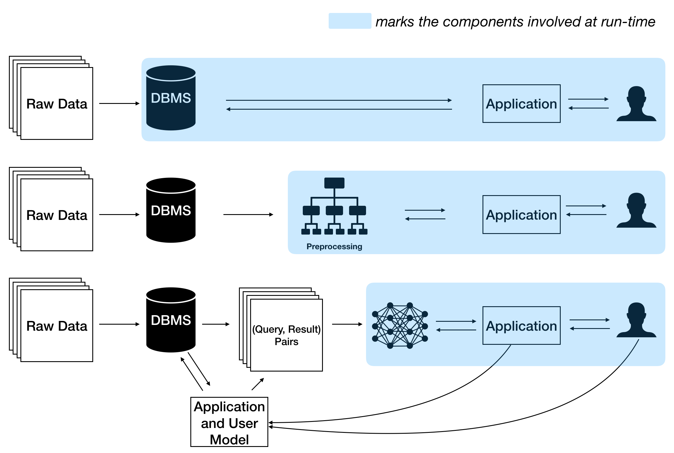
Figure 1: Comparison of systems using traditional database, Datacubes and NeuralCubes.

In this context, our method for learning features of aggregation queries can be viewed as a form of unsupervised learning, where treating query prediction as pretext, the features that we learn along the way can be used for other purposes – in our case exploratory purposes. This is similar to recent techniques in computer vision that learn features using different forms of self supervision, for instance learning to predict spatial context[9, 32], temporal context[44], and perhaps more pertinent to our work, learning to count visual primitives in a scene[33]. These techniques solve certain types of relevant visual tasks that do not require human supervision, but then extract the learned features for supervised learning. Our approach is similar: our training data does not require human intervention, since it is built from existing data cubes techniques, yet the features that we learn from this task can be used to help with visual data exploration.

We also note that there is some very recent work that seeks to combine databases with neural networks. Kraska et al.[22] make the connection between indexing, such as b-trees or hashes, and models, and show that such indexing schemes can be learned using neural networks. Mitzenmacher[31] consider similar learning techniques for Bloom filters. These methods are concerned with using neural networks to speed up computation and minimize memory storage. Although we demonstrate that our method can attain these benefits, the primary focus of our method is in using a neural network as an integral component to visual exploration, i.e. NeuralCubes is not trying to predict any queries that a database can answer.

2 NeuralCubes: Replacing a Database with a Learned Neural Network

We introduce our approach by comparing it with visualization systems that utilizing traditional database and those using advanced preprocessing techniques. Fig. 1 is an overview of these different approaches.

First, we briefly discuss what data queries does a interactive visualization system need. Suppose we are given a set of records, each record contains a set of attributes, and each attribute has a certain type, for instance continuous, categorical, geographic, and temporal, that characterizes the set of values it may take on. Database queries may return a single record, or multiple records, and in the case of the latter it is often of interest to summarize the set of records by performing an aggregation, for instance count, average, or max, depending on the attribute type. Within a visualization system, the set of attributes, their types, and the class of aggregations determine the sorts of queries one may issue that serve as the backbone for visual interaction. For instance, we may perform a group-by query for a given attribute that will return, for each of its values, the result of a specified aggregation, e.g. count. If the attribute type is categorical or temporal, then we can visualize this result as a histogram, whereas if the attribute type is geographic, we may plot the result as a heatmap over a spatial region.

Naively, a visualization system can always issue SQL queries to the database to get the needed information. As summarized in Fig. 2, this approach does support “cold start”, which means no extra processing is needed when the data changes (e.g. adding new records). Besides, there is no need for extra memory other than the data set itself. The results will always be accurate. However, this approach obviously won’t scale when the dataset gets larger, which stops it from being practically used in interactive visualization systems for large dataset.

Many database techniques have been proposed with visualizations in mind. For example, datacubes based proposals[24, 35, 45] are built with the goal of answering aggregational queries in real-time. In particular, they are focused on linked views, such that selection of an attribute in one view updates the visualization of other views, where view updates are based on a set of queries made to the database. Linked views enable the user to engage with the visualization in an iterative process: the user spots a trend in one view, makes a selection based on the trend (i.e. filter on a geographic region), they are presented with updated views in the remaining attributes, and their interaction process repeats. However, these techniques usually requires a large memory footprint and long preprocessing time. While some datacubes based technique can provide absolute correct answer at a given resolution, many sampling based techniques can not guarantee controllable error.

The basic idea behind NeuralCubes is the use of neural networks to learn the process of performing database aggregation queries. It is thus useful to think about the neural network as a function that approximates a database aggregation query, where the input is a data query in the form of a set of attribute ranges, and the output is the aggregation of the data returned from the given input query. The fundamental difference of NeuralCubes with existing techniques is that NeuralCubes is trying to solve the problem in a pure machine learning perspective. Thus NeuralCubes has two modes: offline training and real-time querying. During offline training, we generate query-result pairs and train neural networks to learn to predict results for queries. Then at real-time querying stage, new queries will be evaluated by the trained model to get a predicted result.

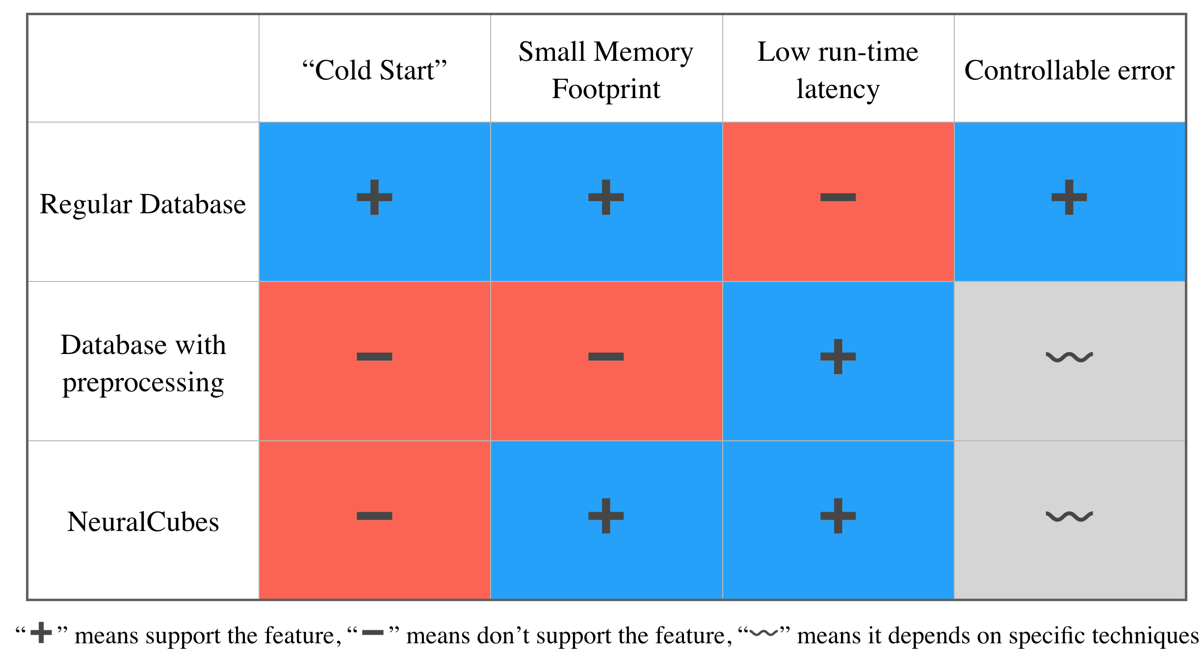
Figure 2: Comparison of supported features of different approaches.

Like most machine learning techniques, the predicted query results from NeuralCubes don’t have a strict error bound. However, we can practically control the error by using neural networks with enough capacity and feeding in a large enough training set. Furthermore, NeuralCubes is designed for visualization. The absolute error is visually neglectable as long as the overall trend and distribution reflects the truth. User can always issue SQL queries to the database to get the accurate numbers.

We summarize the trade-offs of different approaches discussed above in Fig. 2.

2.1 What’s the input of NeuralCubes?

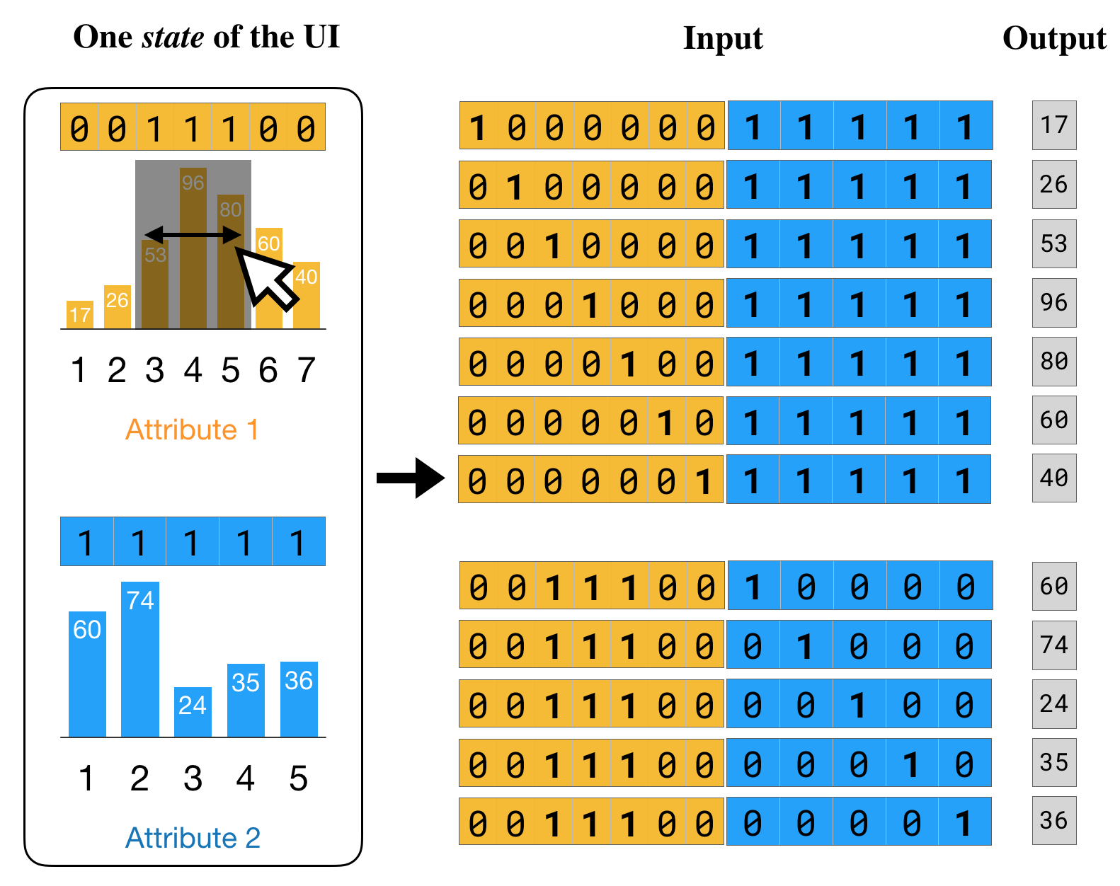
Figure 3: The corresponding input-out pairs for one state of the UI.

We first define the concept of state of a data visualization system. We assume that the underlying database schema has a total of $d$ attributes, where we denote each attribute by $a_{i},1\leq i\leq d$, and we represent the range selection operation for a given attribute $a_{d}$ by $r(a_{d})$. For instance, if an attribute was hour-of-day, then the range operation on this attribute would return a set of hours. At any time, there must be a range selected on each attribute. (No selection on a attribute means select the full range of this attribute.) The set of these ranges of different attributes determine what the plots of each attribute look like. We call this set of ranges a state of the visualization system, denoted as $S={r(a_{1}),r(a_{2}),...r(a_{d})}$. The corresponding query results are $DB(S)\in\mathbb{R}$. Our objective is to train a neural network $f(S)\in\mathbb{R}$ to best approximate $DB$, given training data $D=\left((S_{1},DB(S_{1})),(S_{2},DB(S_{2})),...(S_{n},DB(S_{n}))\right)$, where $S_{i}$ is a state, i.e. $S_{i}=\left(r_{i}(a_{1}),r_{i}(a_{2}),...r_{i}(a_{d})\right)$, and $DB(S_{n})$ is the aggregational result from the database. For example, the state shown in Fig. 3 is $S=\{[3,5],[1,5]\}$.

Then we determine the representation of the range selection that is fed into the network. This is nontrivial due to the different types of attributes, e.g. geographic, temporal, categorical, as well as the types of selections that can be performed on attributes, e.g. spatially contiguous selections in geographic coordinates. To address these challenges in a unified manner, we use many-hot encodings for attribute selections, as shown in Fig. 3. Many-hot encodings are generalizations of one-hot encodings, commonly used as a way to uniquely represent words in neural language models[3], categorical inputs for generative models[10], as well as geographic coordinates for image recognition[42].

More specifically, for a given attribute $a_{i}$ we assume that it may be discretized into $m(a_{i})$ many values. For certain attributes, this assumption is natural: categorical data, temporal data such as hour-of-day or day-of-week, while for continuously-valued data we uniformly discretize the data space into bins. For the attribute’s selection $r(a_{i})$, we then associate a binary vector $\mathbf{r}(a_{i})\in\{0,1\}^{m(a_{i})}$ such that $\mathbf{r}(a_{i})_{j}=1$ if the value at index $j$ belongs to the selection, and $0$ otherwise. This permits arbitrary types of selections for categorical and temporal data. Spatial data, specifically 2D geographic regions, is slightly more complicated: one option is to represent each discretized cell as a single dimension in $\mathbf{r}$, but this would result in a large number of inputs for even small spatial resolutions. We simplify this problem by restrict selections on 2D regions to be rectangular. Thus to represent such a region we associate a pair of vectors $\mathbf{r}^{x}(a_{i})$ and $\mathbf{r}^{y}(a_{i})$ to for the selected x and y intervals, respectively, of the rectangle and then concatenate these two vectors to form the input. In practice, non-rectangular selections can be approximated by issuing multiple rectangular selections.

When generating training set, the ground truth results for the queries are obtained from making actual database queries. At runtime, new queries will be encoded in the same way as in training stage. Then it will be fed into the trained model to get a predicted result.

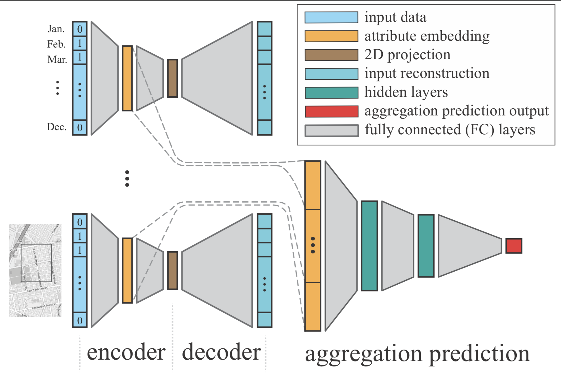
Figure 4: We highlight the general structure of our neural network. For each attribute, we first learn a feature embedding (orange), and then use the embedding for two purposes: we concatenate the embeddings to predict aggregations (red), as well as learn a 2D projection (brown).

2.2 Generating Training Data: Modeling Application and User Interaction

2.2.1 Collecting vs. Generating Training Set

Machine learning models can be seen as a function of the data that they are trained on[21]. It is of integral importance that the training set reflects the goal of the network. In many applications of neural networks such as image classifiers, training data sets must be gathered from the real world, and manually labeled by a large number of human workers[8]. In contrast, since NeuralCubes are used to approximate database queries, a training set can instead be generated by executing queries against a dataset to form ground truth.

2.2.2 Sampling in Input Space vs. User Query Space

When generating a training set, it is important to be careful how the queries are generated. The space of potential queries is exponential in the size of the range of values that can be queried over. But within an information visualization, some queries are much more likely, and thus much more important for the neural network to predict accurately. By choosing a sampling strategy that mirrors the types of queries that will be called by the visualization, we can focus the learning problem on the relevant data distribution.

As discussed in section 2.1, we should randomly generate a state of the UI and then turn it into corresponding queries. Thus, to generate queries, we first generate a range selection for each attribute, e.g. contiguous ranges for temporal or spatial attributes. Then we perform a group by query on one of the attribute with the constrains (range selections) on other attributes, resulting in a batch of query-result pairs for the current attribute. We do the same thing for every attribute, thus giving us all query-result pairs of a state.

In order to sample a range selection over an attribute, there are two strategies we can apply:

1. We can uniformly sample a lower bound of the range from all possible values of the attribute and then uniformly choose a valid upper bound. For example, to generate a range selection for month (represented by integers from $1$ to $12$), we randomly choose a lower bound, say $9$. Then the all possible (exclusive) upper bounds are $10$, $11$, $12$ and $13$. So we just randomly choose one from them, say $11$. Finally this range selection will be $[9,11)$.

2. We can uniformly sample the length of the range from all valid lengths and then uniformly choose a start and end position for that range. Using month as an example again. The possible length of ranges we can make for month are from $1$ to $12$. We randomly choose a length, say $3$. Then, for a length-three range, the possible inclusive starting points/lower bounds are $1,2,3,4,5,6,7,8,9,10$. So we randomly choose one from them, say $2$. Finally this range selection will be $[2,5)$.

The difference between these two strategies is that strategy 1 generates more short-length ranges while strategy 2 generate more long-length ranges. In our experiments, we found people are likely to make queries that has more long-length ranges. An extreme example is the most frequently issued query - the default view for a data visualization dashboard, for which we select full lengths at every attribute. So we apply strategy 2 for all the use cases shown in Section  5.

While it may seem artificial to carefully sample a training set to make the network fit a certain kind of input, it’s important to remember that NeuralCubes is designed, first and foremost, with visualization in mind. Thus, even if we aren’t necessarily learning over the full data distribution of queries, so long as our sampling resembles the manner in which users perform selection, then a user’s interaction with the network should remain meaningful.

2.3 A Neural Network Architecture for Data Queries

Our neural network is composed of a sequence of layers, where a layer is defined as the application of an affine function, followed by applying an elementwise nonlinear function. In this paper we exclusively use fully connected layers. A fully connected layer at index $i$ is parameterized by a weight matrix $\mathbf{W}_{i}\in\mathbb{R}^{b\times a}$ and bias vector $\mathbf{b}_{i}\in\mathbb{R}^{b}$, where it is assumed the previous layer is a vector of length $a$, and the output of the layer produces a vector of length $b$. We denote the affine function at layer $i$ by $g_{i}:\mathbb{R}^{a}\rightarrow\mathbb{R}^{b}$, the nonlinearity by $h_{i}:\mathbb{R}^{b}\rightarrow\mathbb{R}^{b}$, and thus the function $f$ is: $f=h_{n}\circ g_{n}\circ h_{n-1}\circ g_{n-1}\dots h_{1}\circ g_{1}$. Our objective then is to find the sets of parameters, namely the weight matrices and biases, for each layer that result in $f$ being a good approximator of $DB$.

2.3.1 Predicting Aggregations

Our general strategy for predicting aggregations is to learn an embedding for each type of attribute selection, followed by concatenating the attribute embeddings, and then predicting the aggregation query from the concatenation. The intuition behind this architecture is to first learn attribute-specific features that are predictive of aggregation queries, providing us a more informative representation than the input many-hot encodings, and then to combine these features to learn their relationships in predicting the aggregation. We use this general architecture for all of the datasets in the paper, shown in Fig. 4, but tailor the architectures based on the given dataset, which we defer to Section 6. All networks, nonetheless, share the following steps to form the network $f$:

1. Learning Attribute Embeddings. For a given set of attribute selections represented as binary vectors, we first transform each of them separately into their own feature embedding. Namely, for attribute $a_{i}$, let $f_{i}:\mathbb{R}^{m(a_{i})}\rightarrow\mathbb{R}^{d_{i}}$ represent a series of layers that transforms the attribute selection to a $d_{i}$-dimensional embedding space.

2. Attribute Embedding Concatenation. We then concatenate the embeddings into a single vector $\mathbf{\hat{f}}=[f_{1}(\mathbf{r}(a_{1})),f_{2}(\mathbf{r}(a_{2})),...f_{d}(\mathbf{r}(a_{d}))]$, where $\mathbf{\hat{f}}\in\mathbb{R}^{\hat{d}}$, $\hat{d}=\sum_{i=1}^{d}d_{i}$.

3. Aggregation Query Prediction. Given the concatenated embedding $\mathbf{\hat{f}}$, we then feed it through a series of layers, where the last layer outputs a single value, corresponding to the aggregation query. Multiple fully connected layers are used in order to learn the relationship between the attributes, so as to make better predictions.

Prediction Loss. Given the neural network $f$, we can now optimize over its set of parameters to best predict database queries $DB$. For this purpose, we define a loss function for prediction that combines an L1 loss and a mean-squared loss for a given query $Q$:

$$L_{pred}=\lambda_{1}|f(Q)-DB(Q)|+\lambda_{2}(f(Q)-DB(Q))^{2},$$ (1)

where $\lambda_{1}$ and $\lambda_{2}$ weight the contributions of the L1 and mean-squared losses, respectively. The intuition behind this loss is to learn the general trend in the data, captured by the L2 loss, but in order for the training to not be overwhelmed by aggregations that result in very large values, the L1 loss provides a form of robustness.

2.3.2 Autoencoder: Reconstruction as Regularization

Deep neural networks are easy to overfit because they have large amount of parameters. To avoid that, we need add some regularization in training. Reconstruction as regularization has been used in many recent work[20, 37]. We think this approach aligns well with our main goal: we’d like the model to learn the underlying data distribution than memorize the correlation between the noise in the input and the corresponding output. Also, the reconstruction step can provide opportunities for new types of visualization, which we’ll discuss more in section 3.3.

We achieve this by defining an autoencoder[15] for each attribute query $a_{i}$. More specifically, we learn a projection to 2D through a series of layers, starting from the input layer, going to 2D, denoted as an encoder by $\mathbf{e}_{i}:\mathbb{R}^{d_{i}}\rightarrow\mathbb{R}^{2}$. We also want to project back: reconstruct the original query (via its binary representation) from its 2D position, or a decoder $\mathbf{d}_{i}:\mathbb{R}^{2}\rightarrow\mathbb{R}^{m(a_{i})}$. Then the first few layers in the encoder will be shared with the regressor as shown in Fig. 4.

Autoencoder Loss. Since we represent attribute selections as binary-valued, a suitable loss function for measuring the quality of our autoencoder is the binary cross-entropy loss:

$$L_{ae}=-\sum_{j=1}^{m(a_{i})}\left(\mathbf{r}(a_{i})_{j}\log(\mathbf{d}_{i}(\mathbf{e_{i}}(z_{i}))_{j})+(1-\mathbf{r}(a_{i})_{j})\log(1-\mathbf{d}_{i}(\mathbf{e_{i}}(z_{i}))_{j})\right),$$ (2)

where $z_{i}=f_{i}(\mathbf{r}(a_{i}))$ is the feature embedding of the query selection. Note that this loss is defined for each attribute, in order to learn attribute-specific autoencoders.

2.3.3 Combining Together

We combine the prediction loss and the autoencoder loss to learn a function that can both predict queries as well as learn 2D projections of attributes:

$$L=L_{pred}+\lambda_{3}L_{ae},$$ (3)

where $\lambda_{3}$ is a weight giving importance to the autoencoder, relative to the weights on the prediction loss. One can view this objective as a type of multi-task autoencoder[11]: we want to learn an embedding, and a 2D projection, that enables self-reconstruction, while simultaneously learning to predict query aggregations. Importantly, this permits us to contextualize attribute selections with respect to the aggregation task. The prediction task can be viewed as a form of supervision for the 2D projection task, thus attribute selections that result in similar predictions will have similar feature embeddings, as well as similar 2D projections.

3 Using NeuralCubes for Visual Exploration

In this section, we describe how NeuralCubes can be used to build interactive data visualization systems.

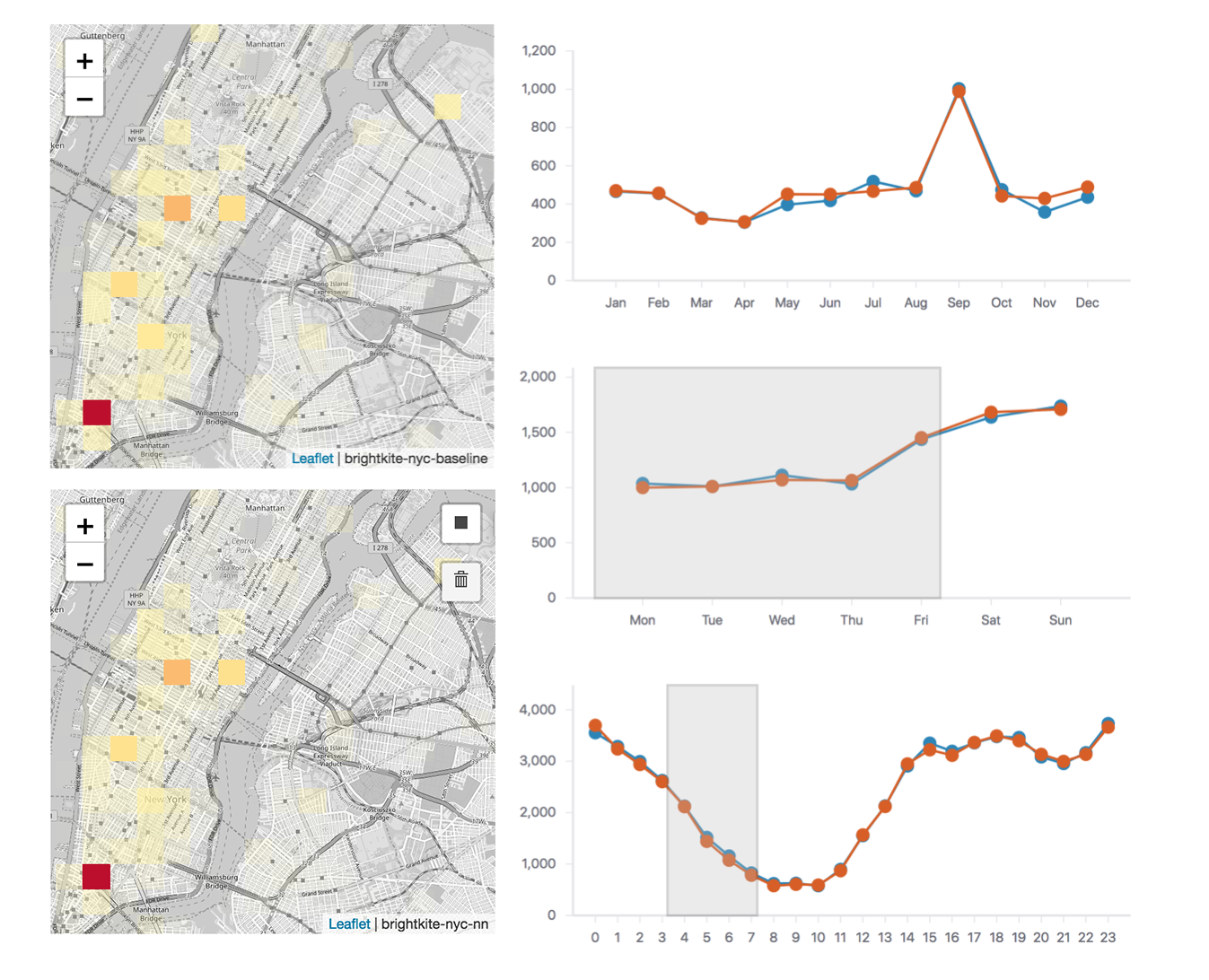
Figure 5: NeuralCubes can be used in a similar fashion to traditional data cubes techniques, allowing us to plot histograms and heatmaps with respect to various attribute selections.

3.1 Plotting Histograms and Heatmaps with NeuralCubes

In traditional data cubes techniques, queries are typically made in order to plot histograms (for 1D attributes) and heatmaps (for 2D attributes). This is typically realized through group by queries, where selections are made for all but one attribute, and then for the held-out attribute, a single query is made to gather aggregations for each of its values, i.e.

SELECT COUNT(*) FROM BrightkiteTable
GROUP_BY dayofweek

NeuralCubes can enable the same type of visual exploration. More specifically, we perform a group by query through our many-hot input encoding, placing a 1 on the attribute value that we would like to query, and a 0 for all other attribute values. Furthermore, we can take advantage of GPU data-parallelism in neural network implementations, and perform this operation in a single mini-batch, providing a significant speed-up through GPU acceleration. Our interface allows the user to perform arbitrary range selections for a given attribute, and enables interactive updates of histograms/heatmaps over the remaining attributes, see Fig. 5 for an illustration.

3.2 Evaluating at Client Side

Another advantage of NeuralCubes is that the trained model is small enough to be sent to client side for evaluation. In comparison, other OLAP datacubes based techniques requires network connections with a backend server for interaction. This advantage of NeuralCubes can be beneficial to both system users and service providers. First, users can expect better experience when making queries. Being able to evaluate at client side, NeuralCubes can eliminate network latency, which is usually a bottleneck. Secondly, service providers can expect much lower cost because the same server can provide service to much more users since Query Per Second (QPS) will be significantly lower than other client-server systems.

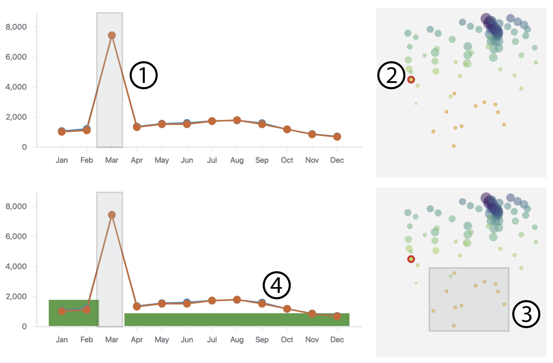
Figure 6: We show how the user can jointly interact with traditional histogram visualizations and latent space visualizations learned by NeuralCubes. On the left we initially show an histogram of counts of social media check-ins dataset of Austin for attribute Month. Upon selecting month March (1), the latent space on the right updates, to reflect this selection (2) (colored by red circular stroke with larger width) and also highlight (colored by red circular stroke with smaller width) all possible selections with the same length of range (which is $1$ in this case). By performing a selection in the latent space (3), the user can explore the frequency of attribute selections (4) that belong to the selected latent space subset.

3.3 Visualizing Attribute Latent Spaces

Although the network can replicate the types of queries perform with data cubes techniques, we can also use different structures that the network learned to enable new forms of visual exploration. In particular, we allow the user to explore the space of attribute selections through each attribute’s learned 2D projection, as discussed in Section 2.3.2. To enable this, we first generate all possible ranges selections for a given attribute, and use the autoencoder to create an overview of their distribution in the 2D space, where we visually encode attributes in a scatterplot. Each point in the latent space view represent a selection of this attribute, where the radius of the point is proportional to its aggregation value, and the color of the point represents the range of the selection, namely the number of values selected in the attribute. Importantly, we ensure that the latent space and the histograms/heatmaps discussed previously in Sec. 3.1 are linked, so that interactions in one view update the other view, see Fig. 6 for an example.

4 Implementation

Software

NeuralCubes is written in Python 3.6 with PyTorch version 0.4. It is implemented in the way that the neural network architecture is dynamically created given a JSON configuration file. When changing a dataset or updating the neural networks, users only need to provide a new JSON configuration. For a given trained model, we utilize it in a Flask http backend server, providing RESTful web services. To test the functionality of evaluating at client side, we converted the model from PyTorch format to TensorFlow format. Then we use TensorFlow.js in client side for model evaluation. We have implemented a web user interface, NeuralCubes Viewer, for interaction, implemented in Javascript using React and React-Vis. In order to make the training set generation faster, we performed ground truth aggregation queries in C++.

Hardware

All the models are trained on a machine with an 8 core Intel i7-7700K 4.20GHz CPU, 32GB main memory, and a Nvidia GTX 1080 Ti GPU with 12GB video memory.

Datasets

A summary of datasets and training/testing statistics of all the case studies is provided in Fig. 7. We evaluated our method on held-out test datasets, generated in the same manner as training data. Testing error is computed as the average L1 norm difference between the predictions and ground truth, scaled by the inverse of the mean of the ground truth set, in order to be commensurable across datasets.

Architectures

While the architectures we used to train the models were all quite similar, there are some distinctions between them that we describe here for the sake of reproducibility. The table in Fig. 8 describes the architectures used in each of the trained models we discuss in this paper.

Mini-Batch

When training neural networks, a mini-batch usually is constructed by randomly choosing a certain number of training samples. However, in practice, we found training is not very stable using this approach for our setup. One of the possible reasons could be the fact that the type of queries are unbalanced in the training set. For example, for an attribute with 10 dimensions, there will be 10 queries needed to plot a line chart for it. For an attribute with 5 dimensions, there will only be 5 queries. Since our training set is generated by selecting the same number of random ranges for each attribute, the number of queries for different attributes will be different. Specifically, attributes with higher dimensionality will have more sample queries than attributes with lower dimensionality. People have proposed solutions like stratified sampling[48] to solve this problem. In this paper, we take advantage of being able to control how we generate the training set and propose a state based mini-batch construction strategy. At training time, a mini-batch will be composed by the corresponding queries of several randomly selected states.

Training

Although we need to tune parameters for each different model, there are some empirical best practice that we found stay stable in our experiments. When choosing the right weights $\lambda_{1},\lambda_{2},\lambda_{3}$, it usually works when setting $\lambda_{1}$ to be $1$. Next, set $\lambda_{2}$ so that $\lambda_{2}L_{1}$ is one or two order of magnitude larger than $\lambda_{1}L_{ae}$. Then set $\lambda_{3}$ so that $\lambda_{3}L_{2}$ is at least two order of magnitude smaller than $\lambda_{2}L_{1}$. Sometimes setting $\lambda_{3}$ to be $0.0$ achieves better performance. When choosing the optimizer for training, we found if we only use mini-batch gradient descent(GD), it’s hard for NeuralCubes to converge. To solve this problem, we used a similar approach as described in[18], which simply use Adam[19] for the first 10 to 20 epochs of training then switch to mini-batch gradient descent. This technique works well for all the training in our experiments.

DataSet	Raw Data Size	# States	M. Size	RAE
B.K. NYC	79k (3.1MB)	10k	703KB	4.25%
B.K Austin	22k (0.8MB)	10k	703KB	3.88%
Flights_Count	5m (204MB)	60k	1.2MB	3.11%
Flights_Delay	5m (204MB)	60k	1.2MB	6.58%
Yellow Cab	12m (1.8GB)	30k	798KB	0.97%
SPLOM	100k (3.9MB)	10k	135KB	2.64%

Figure 7: Summary of training results for the experiments reported in this paper. # States means the number of states used in the training set. M. Size represents the saved file size of trained models. RAE represents Relative Absolute Error, which is calculated as $RAE$ = $\frac{\sum_{i}|\hat{y_{i}}-y_{i}|}{\sum_{i}|y_{i}-\bar{y}|}\times 100\%$, where $\hat{y_{i}}$ is the model’s prediction for query $i$, $y_{i}$ is the ground truth for query $i$, and $\bar{y}$ is the average value of $y_{i}$ in the testing set.

Input	Autoencoder	Regressor
BrightKite
Month (12)	[8, 4, 2, 4, 8]	[220]
Day of Week (7)	[8, 4, 2, 4, 8]
Hour (24)	[12, 6, 2, 6, 12]
Geospatial (40)	[400, 128, 2, 128, 400]
Flights (count)
Month (12)	[120, 20, 2, 20, 120]	[256, 128]
Day of Week (7)	[70, 20, 2, 20, 70]
Hour (24)	[240, 20, 2, 20, 240]
Geospatial (40)	[400, 128, 20, 2, 20, 128, 400]
Carrier (10)	[100, 20, 2, 20, 100]
DelayBin (14)	[140, 32, 2, 32, 140]
Flights (delay)
Month (12)	[120, 20, 2, 20, 120]	[256, 128, 64]
Day of Week (7)	[70, 20, 2, 20, 70]
Hour (24)	[240, 20, 2, 20, 240]
Geospatial (40)	[400, 128, 20, 2, 20, 128, 400]
Carrier (10)	[100, 20, 2, 20, 100]
DelayBin (14)	[140, 32, 2, 32, 140]
Yellow Cab
Month (12)	[120, 20, 2, 20, 120]	[220]
Day of Week (7)	[70, 20, 2, 20, 70]
Hour (24)	[240, 20, 2, 20, 240]
Geospatial (40)	[400, 128, 20, 2, 20, 128, 400]
SPLOM
a0 (#bin)	[16, 8, 2, 8, 16]	[120, 60]
a1 (#bin)	[16, 8, 2, 8, 16]
a2 (#bin)	[16, 8, 2, 8, 16]
a3 (#bin)	[16, 8, 2, 8, 16]
a3 (#bin)	[16, 8, 2, 8, 16]

Figure 8: Architectures for the neural networks used in the experiments with NeuralCubes. The numbers in bold represent attribute embedding layers as described in Fig. 4.

5 Experimental Evaluation

We have explored our method in the context of a variety of datasets, where in this section we highlight quantitative results of our method in predicting aggregations, and qualitative results of our proposed visualization techniques. We note through all results, we show our predictions as orange curves, and the ground truth aggregations in blue curves, in order to consistently compare our method with the actual database queries.

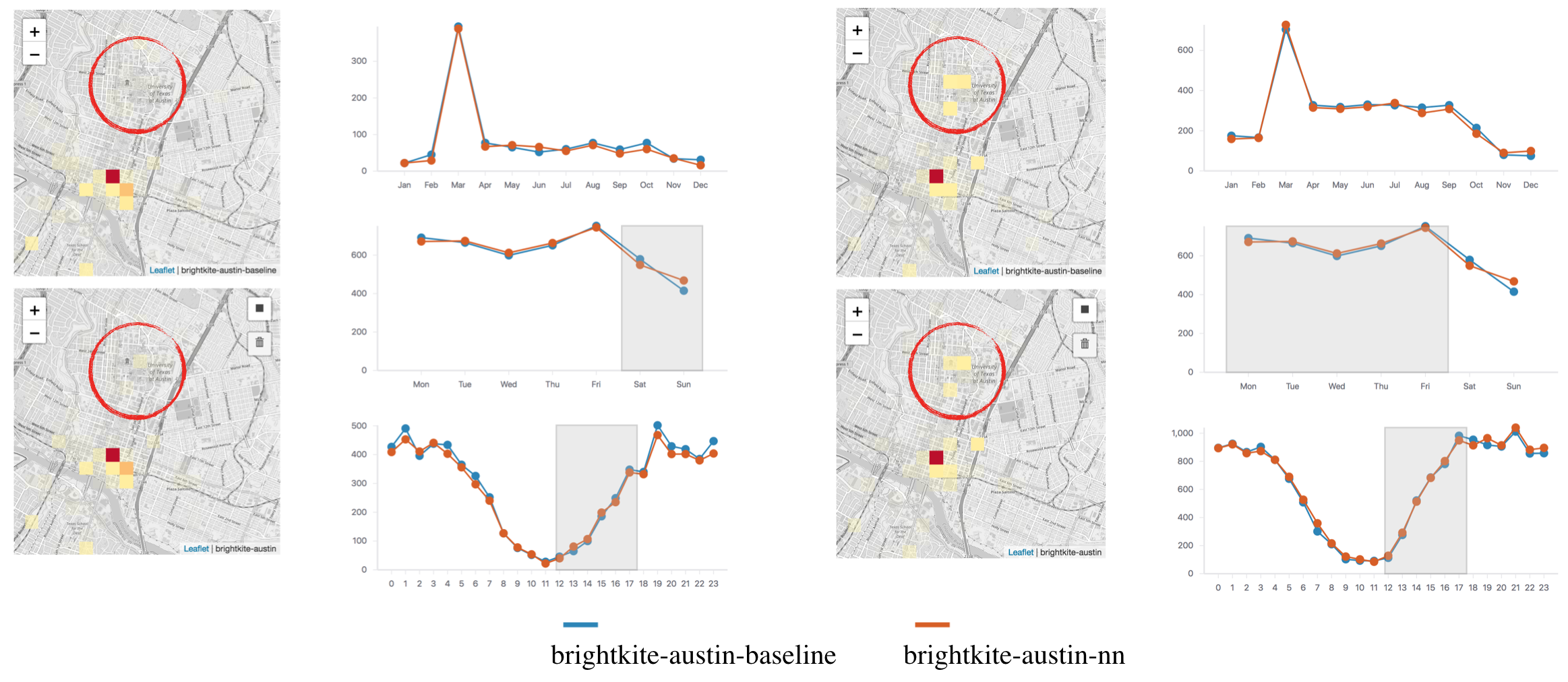
Figure 9: We show how NeuralCubes learned that there are more check-ins on University of Texas at Austin campus during daytime on weekdays.

5.1 Brightkite Social Media Check-ins

Here we study Brightkite[7] social media check-ins to assess the capability of NeuralCubes to learn the count aggregation. Fig. 9 shows examples of how our technique can be treated analogous to a data cubes system, capable of plotting histograms and heatmaps from aggregation queries. We also use this dataset to evaluate training stability and to test the learned latent space contains meaningful information or not.

5.1.1 Training Details

We choose two separate metropolitan areas and train separate networks on each: New York City and Austin. We choose month, day of week, hour, and geospatial information (longitude and latitude) as input dimensions, following common practice in the study of urban activity[24, 29]. The longitude and latitude are encoded as $20+20=40$ bins, following the strategy described in Fig. 3. The weights for L1 loss and L2 loss for regressor and BCE loss for autoencoder are 20, 0.001, and 1 respectively. Each model is trained for 1000 epochs and each epoch takes 6 seconds to train.

5.1.2 Results

The predictions are good for both cities under the same neural network configuration. This shows the generalizability of NeuralCubes.

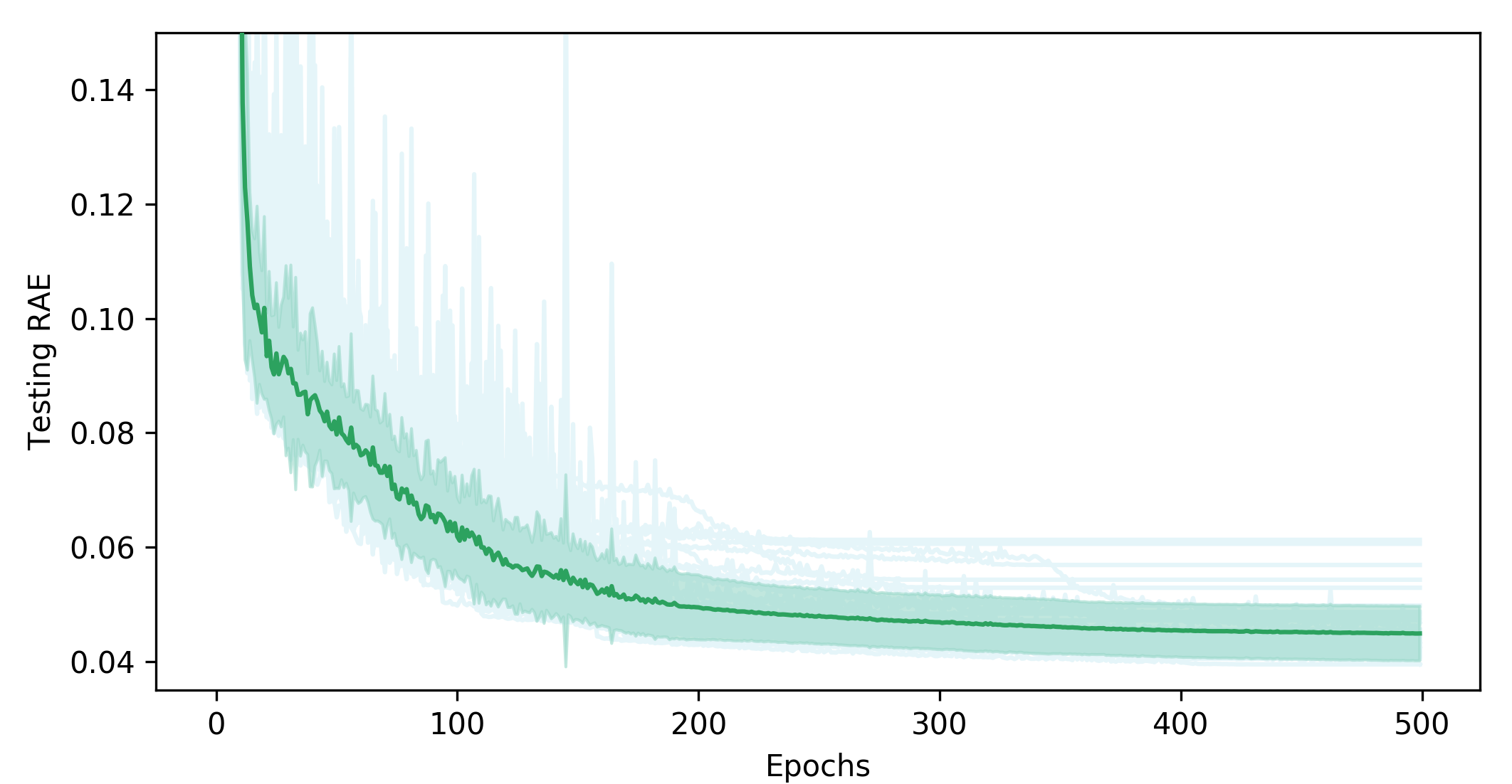
Figure 10: Testing error for 50 independent training on BrightKite NYC dataset with the same configuration. Light green lines represent each individual training. Solid green line represent the mean testing error. Darker green area represent standard deviation from mean. We can notice some variance between different runs. However, all of them eventually converge to relatively the same optimal.

Training Stability

We also evaluated the training stability on BrightKite NYC dataset. Specifically, we independently run 50 training on BrightKite NYC dataset with exactly the same configurations. Then we record the testing error for each model for each epoch. The results are shown in Fig. 10. We can see that NeuralCubes always converge to the same optimal.

Comparing Two Cities by Latent Space

The latent space plots may convey information that could not be directly perceived on histograms of counts. Fig. 11 shows an example. Firstly, the latent space for hour of both cities forms a loop for ranges with same length. This suggests that NeuralCubes learned the fact that hour indeed has a repeated circular pattern. However, the “circle” in Austin’s latent space has a large opening. This could be caused by the difference of lifestyles of the two cities: New York City never sleeps, while Austin goes to bed at night.

5.2 Flight Dataset

We use a dataset collected by the Bureau of Transportation Statistics consisting of flight delay information in the year 2008[34]. For this dataset, our first experiment uses the total flight counts as the aggregation operation. Since this dataset contains an attribute delay time, which is also a meaningful attribute in which to aggregate, our second experiment builds a model to predict the average delay time. Our goal with this model is to check the extent to which NeuralCubes can learn non-monotonic aggregations.

5.2.1 Training Details

Count Predictions

For the count aggregation we filter flights to be within the contiguous United States, and restrict entries to only the 10 most used airlines in the dataset, giving us a total of 5,092,321 entries after removing entries containing missing data. We note that this dataset has more entries and attributes than the Brightkite dataset, including a numeric variable (Delay Time). To encode the numeric variable in our many-hot encoding, we bin the delays in 15 minute increments. The weights for L1 loss, L2 loss and BCE loss are 1, 1e-7, and 1, respectively. Each model is trained for 500 epochs and each epoch takes 160 seconds to train.

Average Predictions

We follow a similar training setup to count, with a couple exceptions. Since generating training samples to predict average delay time itself is very time consuming, we dropped longitude and latitude columns in the raw data and discarded entries whose delay time is smaller than $-60$ minutes or larger than $140$ minutes. The weights for L1 loss, L2 loss and BCE loss are 10, 10, and 1, respectively. Each model is trained for 500 epochs and each epoch takes 160 seconds to train.

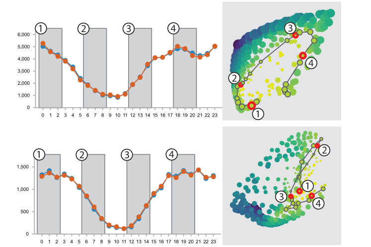
Figure 11: In this figure, we compare the diurnal patterns present in the latent space for “hour” in Austin and NYC. The top half shows the queries and latent space for NYC, while the bottom half shows them for Austin. We highlight the sequence of queries in the latent space for sliding ranges throughout the day, and notice that the activity in New York City is more circular in nature. We find this pattern always exists within multiple independently trained models; though they may have different views (e.g. rotated, stretched) of the latent space due to randomness in the training.

5.2.2 Results

Fig. 7 shows the quantitative results for the two types of aggregation queries. Overall, we find the errors to be competitive, if not lower, than Brightkite, showing that our method is capable of handling different types of attributes, as well as different forms of aggregation. Furthermore, for this dataset note that the size is quite large – 204MB, while the size of our trained networks only occupy 1.2MB for both tasks, demonstrating the significant compression capabilities of our network.

5.3 YellowCab Taxi Dataset

We use NYC YellowCab Taxi trip records of year 2015 from NYC Taxi and Limousine Commission (TLC)[43] to study the learning capacity of NeuralCubes in a series of controlled settings.

5.3.1 Training Details

We choose month, day of week, hour, and pickup location (longitude and latitude) as input dimensions. The longitude and latitude are encoded as $20+20=40$ bins. We created four different datasets under this same schema by sampling 1k records per month, 10k records per month, 100k records per month and 1 million records per month respectively from the original dataset. We refer to these four datasets as YC-1K, YC-10K, YC-100K, and YC-1M respectively. (We performed data cleaning and filtering after sampling. So the actual number of records of each month of a dataset will be slightly less than the sampled number.) As described in Fig. 8, we use the same network configuration for the four datasets. The weights for L1 loss, L2 loss and autoencoder loss are 100.0, 0.0 and 1.0 for YC-1K, YC-10K and YC-100K. For YC-1M, the weights for L1 loss, L2 loss and autoencoder loss are 10.0, 0.0 and 1.0. Each model is trained for 1000 epochs and each epoch takes 15 seconds to train.

Raw Data Size	# States	Model Size	Testing RAE
12k (1.8MB)	30k	798KB	3.70%
120k (18MB)	30k	798KB	2.04%
1.2m (180MB)	30k	798KB	1.35%
12m (1.8GB)	30k	798KB	0.97%

Figure 12: Yellowcab dataset with different raw data size.

Model Size	Training RAE	Testing RAE
113KB	5.06%	5.18%
220KB	3.93%	4.03%
798KB	3.59%	3.70%
1.7MB	2.98%	3.10%

Figure 13: Performance evaluation of different model size (e.g. different number of hidden layers) on the same dataset. In this experiment, we tested four different models on the Yellow Cab 12k dataset.

Training States	Training RAE	Testing RAE
15k	6.74%	6.85%
30k	3.59%	3.70%
60k	3.39%	3.47%

Figure 14: Performance evaluation of different training set size on the same dataset. In this experiment, we tested three different models on the Yellow Cab 12k dataset with different number of states in training sets.

5.3.2 Results

Raw Data Size

We training results for YC-1K, YC-10k, YC-100k and YC-1M are in Fig. 12. We notice a fact that the testing error becomes smaller when the raw data size increase. We think this is due to the fact that when more data are available, there will be less noise. The data distributions that NeuralCubes need to learn will be more smooth, requiring less learning capacity. Since we are using the same neural network configuration, we can expect lower error on dataset that doesn’t require large learning capacity.

Model Size

Another experiment we did is using neural networks with different sizes for the same dataset. We start from a small neural network and then gradually increase the number of hidden layers and neurons to see if the prediction improves. The results are in Fig. 13. Not surprisingly, with larger neural networks, the error reduces.

Training Set Size

Another factor that can influence the training is the size of training set. In this experiment, we tested the same model but with different number of training sets. Results can be found in Fig. 14. We can see a significant accuracy improvement when using 30k training states than 15k training states. However, the improvement from using 30k to 60k is very small. The reason is that the capacity of the neural network may be not enough for 60k training states.

5.4 SPLOM Dataset

Bin Size	# States	Model Size	Testing RAE
10	10k	109KB	1.02%
20	10k	116KB	1.85%
30	10k	122KB	2.25%
40	10k	129KB	2.09%
50	10k	135KB	2.64%

Figure 15: SPLOM dataset with different bin size.

Last, we use the synthetic SPLOM dataset of Kandel et al.[17] to validate whether NeuralCubes can learn how to predict aggregational values under a controlled setting. Since all the attributes of SPLOM dataset are real values, it also provides us an opportunity to study the behavior of NeuralCubes when bin size increases.

Training Details

Following the procedure described in [17], we generated $100,000$ entries of five-attribute records, and divide each attribute into a prescribed number of bins. We trained five different NeuralCubes using 10, 20, 30, 40, and 50 bins respectively. The weights for L1 loss, L2 loss and autoencoder loss are 1.0, 0.0 and 1.0, respectively.

Results

A detailed quantitative evaluation of training NeuralCubes for SPLOM dataset can be found in the table of Fig. 15. As suggested in the table, when we increase the number of bins, the network requires more neurons, and thus a higher capacity, to learn well. We note that the increase in testing error is to be expected, for several reasons. The first reason is that when the bins are refined, few records fall into the same bin. So the variance within each bin is larger, making it more difficult for NeuralCubes to learn the underlying distribution. The second reason is that when the number of bins increase, the space of possible different queries grows exponentially. Yet, we didn’t increase the training set.

6 Discussion

The main limitation in NeuralCubes is the current dependence of the network architecture on the dataset and schema complexity. While we were able to successfully train these networks with a certain amount of experimentation, the process is more cumbersome than we would like. More automated methods to choose among different network architectures are still a current topic of research in machine learning, and beyond the scope of the current paper.

Another limitation is that the output of NeuralCubes are approximations. However, in a visual data exploration system, it is the overall trend and distribution that people mostly want to get. Whenever the user needs the absolute correct answer, they can always query the database for that. The value of NeuralCubes is that it provide a tool for them to quickly find what question they want to ask to the data. Further more, NeuralCubes is designed for visualization. The final results users get are heatmap, line charts, histograms, etc. As long as the error is small, users can hardly tell the difference visually.

One notable feature of NeuralCubes is that the query training set is dependent on the affordances provided by the visual exploration system. This is an advantage in terms of machine learning, because the additional information available allows us to simplify the problem of training a network capable of answering any query. At the same time, the fact that we have full control over the training set of queries is sometimes a disadvantage, because a poorly-generated training set can cause the training procedure to fail. Our proof-of-concept system shows the advantages that a neural network provides in the context of a visual exploration system, but a thorough study on how to generate appropriate training sets remains a topic for future work.

7 Conclusion and Future Work

We believe that the main value of NeuralCubes lies in its ability to learn high-level features of the dataset from which powerful visual data exploration techniques become possible. While the accuracy of the approximated results seems well within what is to be expected of a neural network, we warn against expecting that NeuralCubes would be able to learn minute details of the dataset. Liu et al.[26] distinguished between approximate, sampling-based systems and exact aggregation systems. We would consider NeuralCubes to be approximate as well, but approximate in its aggregations; it trades exact accuracy of the answer for higher-level knowledge about the queries to be answered.

We remain enthusiastic about the future of connecting interactive information visualization and machine learning. We are particularly interested in solving the above two problems by leveraging recent work in user modeling and predictive interaction[2]. The better we can predict how people (through a particular UI) make queries against a DB in a visual exploration scenario, the more effectively we will be able to train NeuralCubes’s networks.

Because the process of aggregating queries is a differentiable function, this opens up several opportunities, such as query sensitivity and the discovery of queries that lead to user-prescribed aggregations. We are excited to explore these research avenues as part of future work.

References

- [1] S. Agarwal, B. Mozafari, A. Panda, H. Milner, S. Madden, and I. Stoica. Blinkdb: queries with bounded errors and bounded response times on very large data. In Proceedings of the 8th ACM European Conference on Computer Systems, pp. 29–42. ACM, 2013.
- [2] L. Battle, R. Chang, and M. Stonebraker. Dynamic prefetching of data tiles for interactive visualization. In Proceedings of the 2016 International Conference on Management of Data, pp. 1363–1375. ACM, 2016.
- [3] Y. Bengio, R. Ducharme, P. Vincent, and C. Jauvin. A neural probabilistic language model. Journal of machine learning research, 3(Feb):1137–1155, 2003.
- [4] A. Bilal, A. Jourabloo, M. Ye, X. Liu, and L. Ren. Do convolutional neural networks learn class hierarchy? IEEE transactions on visualization and computer graphics, 24(1):152–162, 2018.
- [5] D. Cashman, G. Patterson, A. Mosca, and R. Chang. Rnnbow: Visualizing learning via backpropagation gradients in recurrent neural networks. In Workshop on Visual Analytics for Deep Learning (VADL), 2017.
- [6] S.-M. Chan, L. Xiao, J. Gerth, and P. Hanrahan. Maintaining interactivity while exploring massive time series. In Visual Analytics Science and Technology, 2008. VAST’08. IEEE Symposium on, pp. 59–66. IEEE, 2008.
- [7] E. Cho, S. A. Myers, and J. Leskovec. Friendship and mobility: user movement in location-based social networks. In Proceedings of the 17th ACM SIGKDD international conference on Knowledge discovery and data mining, pp. 1082–1090. ACM, 2011.
- [8] J. Deng, W. Dong, R. Socher, L.-J. Li, K. Li, and L. Fei-Fei. Imagenet: A large-scale hierarchical image database. In Computer Vision and Pattern Recognition, 2009. CVPR 2009. IEEE Conference on, pp. 248–255. IEEE, 2009.
- [9] C. Doersch, A. Gupta, and A. A. Efros. Unsupervised visual representation learning by context prediction. In The IEEE International Conference on Computer Vision (ICCV), December 2015.
- [10] A. Dosovitskiy, J. T. Springenberg, and T. Brox. Learning to generate chairs with convolutional neural networks. In Computer Vision and Pattern Recognition (CVPR), 2015 IEEE Conference on, pp. 1538–1546. IEEE, 2015.
- [11] M. Ghifary, W. Bastiaan Kleijn, M. Zhang, and D. Balduzzi. Domain generalization for object recognition with multi-task autoencoders. In Proceedings of the IEEE international conference on computer vision, pp. 2551–2559, 2015.
- [12] J. Gray, S. Chaudhuri, A. Bosworth, A. Layman, D. Reichart, M. Venkatrao, F. Pellow, and H. Pirahesh. Data cube: A relational aggregation operator generalizing group-by, cross-tab, and sub-totals. Data mining and knowledge discovery, 1(1):29–53, 1997.
- [13] V. Harinarayan, A. Rajaraman, and J. D. Ullman. Implementing data cubes efficiently. In Acm Sigmod Record, vol. 25, pp. 205–216. ACM, 1996.
- [14] G. Hinton, L. Deng, D. Yu, G. E. Dahl, A.-r. Mohamed, N. Jaitly, A. Senior, V. Vanhoucke, P. Nguyen, T. N. Sainath, et al. Deep neural networks for acoustic modeling in speech recognition: The shared views of four research groups. IEEE Signal Processing Magazine, 29(6):82–97, 2012.
- [15] G. E. Hinton and R. R. Salakhutdinov. Reducing the dimensionality of data with neural networks. Science, 313(5786):504–507, 2006.
- [16] N. Kamat, P. Jayachandran, K. Tunga, and A. Nandi. Distributed and interactive cube exploration. In Data Engineering (ICDE), 2014 IEEE 30th International Conference on, pp. 472–483. IEEE, 2014.
- [17] S. Kandel, R. Parikh, A. Paepcke, J. M. Hellerstein, and J. Heer. Profiler: Integrated statistical analysis and visualization for data quality assessment. In Proceedings of the International Working Conference on Advanced Visual Interfaces, pp. 547–554. ACM, 2012.
- [18] N. S. Keskar and R. Socher. Improving generalization performance by switching from adam to sgd. arXiv preprint arXiv:1712.07628, 2017.
- [19] D. P. Kingma and J. Ba. Adam: A method for stochastic optimization. arXiv preprint arXiv:1412.6980, 2014.
- [20] D. P. Kingma, S. Mohamed, D. J. Rezende, and M. Welling. Semi-supervised learning with deep generative models. In Advances in neural information processing systems, pp. 3581–3589, 2014.
- [21] P. W. Koh and P. Liang. Understanding black-box predictions via influence functions. arXiv preprint arXiv:1703.04730, 2017.
- [22] T. Kraska, A. Beutel, E. H. Chi, J. Dean, and N. Polyzotis. The case for learned index structures. arXiv preprint arXiv:1712.01208, 2017.
- [23] A. Krizhevsky, I. Sutskever, and G. E. Hinton. Imagenet classification with deep convolutional neural networks. In F. Pereira, C. J. C. Burges, L. Bottou, and K. Q. Weinberger, eds., Advances in Neural Information Processing Systems 25, pp. 1097–1105. Curran Associates, Inc., 2012.
- [24] L. Lins, J. T. Klosowski, and C. Scheidegger. Nanocubes for real-time exploration of spatiotemporal datasets. IEEE Transactions on Visualization and Computer Graphics, 19(12):2456–2465, 2013.
- [25] M. Liu, J. Shi, Z. Li, C. Li, J. Zhu, and S. Liu. Towards better analysis of deep convolutional neural networks. IEEE transactions on visualization and computer graphics, 23(1):91–100, 2017.
- [26] Z. Liu, B. Jiang, and J. Heer. immens: Real-time visual querying of big data. In Computer Graphics Forum, vol. 32, pp. 421–430. Wiley Online Library, 2013.
- [27] J. Mackinlay. Automating the design of graphical presentations of relational information. ACM Transactions On Graphics, 5(2):110–141, 1986.
- [28] J. Mackinlay, P. Hanrahan, and C. Stolte. Show me: Automatic presentation for visual analysis. IEEE transactions on visualization and computer graphics, 13(6), 2007.
- [29] F. Miranda, H. Doraiswamy, M. Lage, K. Zhao, B. Gonçalves, L. Wilson, M. Hsieh, and C. T. Silva. Urban pulse: Capturing the rhythm of cities. IEEE transactions on visualization and computer graphics, 23(1):791–800, 2017.
- [30] F. Miranda, L. Lins, J. T. Klosowski, and C. T. Silva. Topkube: a rank-aware data cube for real-time exploration of spatiotemporal data. IEEE transactions on visualization and computer graphics, 24(3):1394–1407, 2018.
- [31] M. Mitzenmacher. A model for learned bloom filters and related structures. arXiv preprint arXiv:1802.00884, 2018.
- [32] M. Noroozi and P. Favaro. Unsupervised learning of visual representations by solving jigsaw puzzles. In European Conference on Computer Vision, pp. 69–84. Springer, 2016.
- [33] M. Noroozi, H. Pirsiavash, and P. Favaro. Representation learning by learning to count. In The IEEE International Conference on Computer Vision (ICCV), Oct 2017.
- [34] B. of Transportation Statistics. On-time performance. http://www.transtats.bts.gov/Fields.asp?Table ID=236. Accessed: 2018-03-29.
- [35] C. A. Pahins, S. A. Stephens, C. Scheidegger, and J. L. Comba. Hashedcubes: Simple, low memory, real-time visual exploration of big data. IEEE transactions on visualization and computer graphics, 23(1):671–680, 2017.
- [36] N. Pezzotti, T. Höllt, J. Van Gemert, B. P. Lelieveldt, E. Eisemann, and A. Vilanova. Deepeyes: Progressive visual analytics for designing deep neural networks. IEEE transactions on visualization and computer graphics, 24(1):98–108, 2018.
- [37] S. Sabour, N. Frosst, and G. E. Hinton. Dynamic routing between capsules. In Advances in neural information processing systems, pp. 3856–3866, 2017.
- [38] Y. Sismanis, A. Deligiannakis, N. Roussopoulos, and Y. Kotidis. Dwarf: Shrinking the petacube. In Proceedings of the 2002 ACM SIGMOD international conference on Management of data, pp. 464–475. ACM, 2002.
- [39] C. Stolte, D. Tang, and P. Hanrahan. Polaris: A system for query, analysis, and visualization of multidimensional relational databases. IEEE Transactions on Visualization and Computer Graphics, 8(1):52–65, 2002.
- [40] H. Strobelt, S. Gehrmann, H. Pfister, and A. M. Rush. Lstmvis: A tool for visual analysis of hidden state dynamics in recurrent neural networks. IEEE transactions on visualization and computer graphics, 24(1):667–676, 2018.
- [41] I. Sutskever, O. Vinyals, and Q. V. Le. Sequence to sequence learning with neural networks. In Advances in neural information processing systems, pp. 3104–3112, 2014.
- [42] K. Tang, M. Paluri, L. Fei-Fei, R. Fergus, and L. Bourdev. Improving image classification with location context. In Proceedings of the IEEE international conference on computer vision, pp. 1008–1016, 2015.
- [43] N. Taxi and L. Commission. Yellowcab taxi trip records. http://www.nyc.gov/html/tlc/html/about/trip_record_data.shtml. Accessed: 2018-09-14.
- [44] X. Wang and A. Gupta. Unsupervised learning of visual representations using videos. In The IEEE International Conference on Computer Vision (ICCV), December 2015.
- [45] Z. Wang, N. Ferreira, Y. Wei, A. S. Bhaskar, and C. Scheidegger. Gaussian cubes: Real-time modeling for visual exploration of large multidimensional datasets. IEEE transactions on visualization and computer graphics, 23(1):681–690, 2017.
- [46] E. Wu, L. Battle, and S. R. Madden. The case for data visualization management systems: vision paper. Proceedings of the VLDB Endowment, 7(10):903–906, 2014.
- [47] M. Zaharia, M. Chowdhury, M. J. Franklin, S. Shenker, and I. Stoica. Spark: Cluster computing with working sets. 2010.
- [48] P. Zhao and T. Zhang. Accelerating minibatch stochastic gradient descent using stratified sampling. arXiv preprint arXiv:1405.3080, 2014.