Abstract

This paper aims to better predict highly skewed auto insurance claims by combining candidate predictions. We analyze a version of the Kangaroo Auto Insurance company data and study the effects of combining different methods using five measures of prediction accuracy. The results show the following. First, when there is an outstanding (in terms of Gini Index) prediction among the candidates, the “forecast combination puzzle” phenomenon disappears. The simple average method performs much worse than the more sophisticated model combination methods, indicating that combining different methods could help us avoid performance degradation. Second, the choice of the prediction accuracy measure is crucial in defining the best candidate prediction for “low frequency and high severity” (LFHS) data. For example, mean square error (MSE) does not distinguish well between model combination methods, as the values are close. Third, the performances of different model combination methods can differ drastically. We propose using a new model combination method, named ARM-Tweedie, for such LFHS data; it benefits from an optimal rate of convergence and exhibits a desirable performance in several measures for the Kangaroo data. Fourth, overall, model combination methods improve the prediction accuracy for auto insurance claim costs. In particular, Adaptive Regression by Mixing (ARM), ARM-Tweedie, and constrained Linear Regression can improve forecast performance when there are only weak learners or when no dominant learner exists.

1 1 0 Academic Editor: Marc S. Paolella 10 June 2021 6 April 2022 8 April 2022 https://doi.org/ Combining Predictions of Auto Insurance Claims Combining Predictions of Auto Insurance Claims Chenglong Ye ^1,*, Lin Zhang ², Mingxuan Han ³, Yanjia Yu ⁴, Bingxin Zhao ⁴ and Yuhong Yang ⁴ Chenglong Ye, Lin Zhang, Mingxuan Han, Yanjia Yu, Bingxin Zhao, Yuhong Yang Ye, Chenglong, Lin Zhang, Mingxuan Han, Yanjia Yu, Bingxin Zhao, and Yuhong Yang Correspondence: chenglong.ye@uky.edu

1 Introduction

The average countrywide insurance expenditure tends to rise from year to year. Analyzing insurance data to predict future insurance claim costs is of enormous interest to the insurance industry. In particular, the accurate prediction of claim cost is fundamental in determining policy premiums, as it prevents potentially losing customers due to overcharging and potential loss of profits due to undercharging.

Non-life insurance data are distinct from common regression data due to their “low frequency and high severity” (LFHS) characteristic—i.e., the distribution of the claim cost is highly right-skewed and features a large point mass at zero. This paper focuses on improving the prediction accuracy for such insurance data by model combination/averaging.

Researchers have developed various methods for analyzing insurance data in recent decades. Bailey and Simon (1960) proposed the minimum bias procedure as an insurance pricing technique for multi-dimensional classification. However, the minimum bias procedure lacks a statistical evaluation of the model. See Feldblum and Brosius (2003) for a detailed overview of the minimum bias procedure and its extensions. In the late 1990s, the generalized linear models (GLM) framework (Nelder and Wedderburn, 1972) was applied to model the insurance data; this is now the standard method used in the insurance industry for modeling claim costs. Jørgensen and Paes De Souza (1994) proposed the classical compound Poisson–Gamma model, which assumes the number of claims to follow a Poisson distribution and be independent of the average claim cost that has a Gamma distribution. Gschlößl and Czado (2007) extended this approach and allowed dependency between the number of claims and the claim size through a fully Bayesian approach. Smyth and Jørgensen (2002) used double generalized linear models for the case where we only observe the claim cost but not the frequency. Many authors have proposed methods for insurance pricing using different frameworks other than GLM, including quantile regression (Heras et al., 2018), hierarchical modeling (Frees and Valdez, 2008), machine learning (Kašćelan et al., 2015; Yang et al., 2016), the copula model (Czado et al., 2012), and the spatial model (Gschlößl and Czado, 2007).

Given the availability of many useful statistical models, empirical evidence has shown that combining models, in general, is a robust and effective way to improve predictive performance. Many works have improved the prediction accuracy by combining different models, which can be different types of models or same-type models with different tuning parameters. For instance, Wolpert (1992) proposed the use of Stacked Generalization to take prediction results from the first-layer base learners as meta-features to produce model-based combined forecasts in the second layer. A gradient-boosting machine (Friedman, 2001), known as greedy function approximation, suggests that using a weighted average of many weak learners can produce an accurate prediction. Yang (2001) proposed performing adaptive regression by mixing (ARM), a weighted average method that works well for both parametric and nonparametric regression with an unknown error variance. Hansen and Racine (2012) proposed Jackknife model averaging, which involves a linearly weighted average of linear estimators searching for the optimal weight of each base regression model. Zhang et al. (2016) proposed the use of a weight choice criterion for optimal estimation in generalized linear models. We refer readers to Wang et al. (2014) for a detailed literature review on the theory and methodology of model combination.

However, in the specific context of insurance data, little research has been carried out on combining predictions, except for Ohlsson (2008); Sen et al. (2018). In particular, Sen et al. (2018) proposed a method to merge some levels of a categorical predictor in the model, which is a pre-step of applying model averaging. Ohlsson (2008) proposed to combine the generalized linear model and the credibility model, with special focus on the car model classification problem for auto insurance. These two works are not directly related to combining predictions generated from different models for highly zero-inflated insurance data. To the best of our knowledge, no previous work has been done. Given the apparent importance of accurately predicting insurance claim costs, we propose a model combination method to capture such data characteristics.

Our paper focuses on improving the prediction accuracy of individual models/predictions by combining multiple predictions. We investigate how different model combination methods perform under different measures of prediction accuracy for LFHS data. We propose a model combination method named ARM-Tweedie, assuming the claim cost follows a Tweedie distribution. The Tweedie distribution family includes both continuous distributions (e.g., normal, Inverse Gaussian, gamma) and discrete distributions (e.g., Poisson, compound Poisson-gamma). In particular, we use the compound Poisson-gamma distribution in the Tweedie family (with the parameter $1<p<2$) since it allows a mixture of zeros and positive continuous numbers. It is a popular choice in the application of claim cost modeling.

The contributions of this paper are threefold. First, we design a novel model combination method for zero-inflated non-negative response data, where most current model combination methods fail to capture such a characteristic in theory. Second, we show that our method achieves the optimal rate of convergence offered by the candidates. From the risk-bound perspective, our method adapts to the optimal estimation of the mean function. Third, the conclusions of our analysis on a real-life data set provide both tools and guidance, especially to practitioners, on applying model combination methods to claim cost data for both adaptation and improvement.

More specifically, we try to answer several interesting questions: Do model combination methods improve over the best candidate prediction for insurance data? Is the so-called “forecast combination puzzle” (Stock and Watson, 2004; Qian et al., 2019) still relevant when dealing with insurance data? Under different measures of prediction accuracy, which model combination methods work the best? We carry out a real-data analysis in this work. Thirteen analysts participated by building models to predict the claim cost of each insurance policy in a holdout data set. Based on their predictions, we apply different model combination methods to obtain new predictions in the hope of achieving a higher prediction accuracy. Different measures of prediction accuracy are considered due to the existence of various constraints or preferences in practice. For example, a reasonable prediction should identify the most costly customer and provide the correct scale of the claim amount. Specifically, our paper includes five measures: mean absolute error, root-mean-square error, rebalanced root-mean-square error, the relative difference between the total predicted cost and the actual total cost, and the Normalized Gini index.

The remainder of this paper is organized as follows. We describe the general methodology in Section 2, a data summary in Section 2.1, a description of the project in Section 2.2, and the measures of performance in Section 2.3. Section 3 describes the performance of the predictions provided by the analysts. The results of the model combination methods are given in Section 4, while we introduce the proposed ARM-Tweedie method in Section 4.1.2. We end our paper with a discussion in Section 5. The proof of the main theoretical result is included in Appendix A.

2 General Methodology

In this section, we provide a detailed description of our research methodology.

2.1 Data Summary

The Kangaroo Auto Insurance data (De Jong and Heller, 2008) is based on one-year vehicle insurance policies written in 2004 or 2005. The original data set is downloadable from the R package “insuranceData”. We added a random noise to each continuous variable before releasing them to the data analysts. The perturbed data are available upon request. There are 67,856 policies and 10 variables in this dataset. The variable information is presented in Table 1.

Table 1: Variable description of the Kangaroo dataset. The variables in bold are directly related to the claim cost. The number in parentheses is the variance ratio (variance of perturbed ones to that of unperturbed ones) of each continuous variable. For the response claimcost0, noise is only added to the positive values.

Variable	Description	Variable	Description
veh_value	(1.10) Vehicle value	gender	The gender of the driver
veh_body	The type of the vehicle body	area	Driver’s area of residence
veh_age	The age group of the vehicle	agecat	Driver’s age group
claimcst0	(1.23) Total claim amount	exposure	(0.91) The covered period
numclaims	Number of claims	clm	Indicator if at least one claim

2.2 Project Description

We demonstrated the performance of the different model combination methods for the Kangaroo data through the following procedure.

1. (Data Process) The dataset was split into 3 parts: 22,610 observations for Training, 22,629 observations for Validation, and 22,617 observations for Holdout;

2. (Prediction) Using only the training data, 13 analysts built their models to predict the “total amount of claims” (claimcst0). We refer to these predictions made by the analysts as candidate predictions;

3. (Model Combination) We applied different model combination methods on the 13 candidate prediction models from step 2 and trained the model averaging weights using a subset (5000 observations) of the validation set.

4. (Evaluation) Finally, based on the holdout set, different predictive performance measures were calculated for both the candidate predictions and the combined predictions using model combination methods.

It is worth pointing out that 94% of the claim costs have the value of zero (no claims) in the training set. We present a histogram and a Lorenz curve (Lorenz, 1905) (the cumulative proportion of the claim amount against the cumulative proportion of insurers) of the training set in Figure 1. For the non-zero claims, the distribution is right-skewed and heavy-tailed.

In our description, it seems that not all the observations in the validation set are used. Indeed, in step 2, we used the validation set to evaluate the prediction accuracy of the candidate predictions. Then, the analysts modified their models (they may also choose not to modify their models). More accurately, the candidate predictions refer to the predictions made after such modifications have taken place. For more details, see Section 4.2. In addition, the performances of the 13 candidate predictions evaluated using the 5000 random observations in step 3 are similar to the performances on the holdout set, verifying the reasonability of using a sample of size 5000 to train the weights.

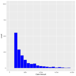
(a)

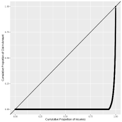
(b)

Figure 1: Data summary of the training set. Left panel: histogram of the training set. There is a massive spike at 0 with a frequency of 21,076, which is not plotted due to space limitations. Right panel: Lorenz Curve of the training set.

2.3 Measure of Prediction Accuracy

Let $n_{e}$ be the number of policies in the evaluation set. Denote $y_{i}$ and $\hat{y}_{i}$ as the claim cost and the predicted claim cost, respectively, for the $i$-th policy. We consider the following five measures of the prediction accuracy of $\{\hat{y}_{i}\}_{i=1}^{n_{e}}$.

Gini Index

Gini index (Gini, 1912), based on the ordered Lorenz curve, is a well-accepted tool for evaluating the performance of auto insurance claim predictions. There are many variants of the Gini index. The one we utilize here is slightly different from those considered in Frees et al. (2014).

For a sequence of numbers $\{s_{1},\dots,s_{n_{e}}\}$, let $\mbox{R}\left(s_{i}\right)\in\{1,\dots,n_{e}\}$ be the rank of $s_{i}$ in the sequence ($\mbox{R}\left(s_{i}\right)<\mbox{R}(s_{j})$ if $s_{i}<s_{j}$, given no ties exist. The tie-breaking method is discussed in Remark 2.3). The normalized Gini index is referred to as:

$$G=\dfrac{\sum_{i=1}^{n_{e}}y_{i}\mbox{R}\left(\hat{y}_{i}\right)\left/\sum_{i=1}^{n_{e}}y_{i}\right.-\sum_{i=1}^{n_{e}}\frac{n_{e}-i+1}{n_{e}}}{\sum_{i=1}^{n_{e}}y_{i}\mbox{R}\left(y_{i}\right)\left/\sum_{i=1}^{n_{e}}y_{i}\right.-\sum_{i=1}^{n_{e}}\frac{n_{e}-i+1}{n_{e}}}.$$ (1)

In (1), the Gini index depends on the predictions of $\{y_{i}\}_{i=1}^{n_{e}}$ only through their relative orders. Using some easy algebra, we obtain: $\sum_{i=1}^{n_{e}}y_{i}\mbox{R}\left(y_{i}\right)\geq\sum_{i=1}^{n_{e}}y_{i}\mbox{R}\left(\hat{y}_{i}\right)$ and $\sum_{i=1}^{n_{e}}y_{i}\mbox{R}\left(y_{i}\right)+\sum_{i=1}^{n_{e}}y_{i}\mbox{R}\left(\hat{y}_{i}\right)\geq(n_{e}+1)\sum_{i=1}^{n_{e}}y_{i}$, with $\sum_{i=1}^{n_{e}}[y_{i}\mbox{R}\left(y_{i}\right)/\sum_{i=1}^{n_{e}}y_{i}]-\sum_{i=1}^{n_{e}}(n_{e}-i+1)/n_{e}>0$. Therefore, we have $-1\leq G\leq 1$, where the equality holds at $\mbox{R}\left(y_{i}\right)=\mbox{R}\left(\hat{y}_{i}\right)$ or $\mbox{R}\left(y_{i}\right)+\mbox{R}\left(\hat{y}_{i}\right)=n_{e}+1$, respectively.

Unlike the other measures we consider, a prediction with a larger Gini index (closer to 1) is favored. To break the ties when calculating the order, we set $R(y_{i})>R(y_{j})$ if $y_{i}=y_{j},\ i<j$.

2.4 Root-Mean-Square Error (RMSE) and Mean Absolute Error (MAE)

Root-mean-square error and mean absolute error are defined as $\sqrt{\frac{1}{n_{e}}\Sigma_{i=1}^{n_{e}}(y_{i}-\hat{y}_{i})^{2}}$ and $\frac{1}{n_{e}}\Sigma_{i=1}^{n_{e}}|y_{i}-\hat{y}_{i}|$, respectively.

Whatever the determination of the policy premiums is, the insurance company needs to make profits and thus cares about the difference between the total cost and the predicted total cost. Below, we consider two measures of prediction accuracy that consider the overall scale of the prediction.

2.4.1 Rebalanced Root-Mean-Square Error (Re-RMSE)

Let $\lambda=\frac{\Sigma y_{i}}{\Sigma\hat{y}_{i}}$ be the scale parameter. Then, the rebalanced root-mean-square error is defined as $\sqrt{\frac{1}{n_{e}}\Sigma_{i=1}^{n_{e}}(y_{i}-\lambda\hat{y}_{i})^{2}}$; this is the root-mean-square error of the scaled/rebalanced prediction $\lambda\hat{y}_{i}$, whose total predicted cost is equal to the actual total claim cost.

2.4.2 SUM Error

Here, we define (relative) SUM error as $\Sigma_{i=1}^{n_{e}}(\hat{y}_{i}-y_{i})/\Sigma_{i=1}^{n_{e}}y_{i}$, which is the relative difference between the total predicted cost and the actual total cost. SUM error is a way to measure the deviance of the total predicted claim cost from the actual total claim cost. Note that a SUM error with a small absolute value is preferred.

3 Performances of the Candidate Predictions

The 13 candidate predictions can be categorized into two types. One type is based on distinct predictions of the number of claims (frequency) and the claim cost (severity). This approach typically generates predictions with values of zero. The other type directly predicts the claim cost, typically producing many small non-zero-valued predictions. Four out of the 13 candidate predictions belong to the first type (distinct predictions).

Table 2 shows the performances of the 13 candidate predictions. We also provide in Table 3 the partial correlation matrix of the candidate predictions given the true value of the response. No prediction outperformed all its competitors in every measure of prediction accuracy. For instance, A5 has the largest/worst RMSE among all the predictions, while its Gini index (0.95) is overwhelmingly better than that of any other analyst (none of the values are more than 0.26). The MAE values of the predictions are closely related to SUM. Since the response $\{y_{i}\}_{i=1}^{n_{e}}$ contains too many zeros, a prediction $\{\hat{y}_{i}\}_{i=1}^{n_{e}}$ will have a relatively small MAE if $\max\{y_{i}\}$ is small, such as A1 with a SUM around $-$1. For the SUM error, most predictions have negative values, except A5. Specifically, the SUM errors of A1 and A2 almost reach $-$1. We checked the predictions of A1 and A2 and found that all the predicted values were less than 10. In practice, it is unreasonable to use such small-scale values as a final prediction of the claim cost, even with their acceptable performance on MAE and Gini. Thus, we suggest the use of more than one measure of prediction accuracy in this context.

Table 2: Performance of the combined predictions. The highlighted values in each column indicate the best model combination method for each scenario. We also provide the estimated standard error of MAE, RMSE, and Re-RMSE to understand their reliability. The bold means the best performance among the 13 preditctions for each prediction measure. The N/A is because the combined prediction based on QR uses 0 as the prediction for every observation, so the scale parameter in Re-RMSE does not exist.

Predictions	MAE	RMSE	Re_RMSE	Gini	SUM
A1	149.93 (7.49)	1136.00 (65.71)	1125.41 (65.57)	0.1956	$-$1.00
A2	154.08 (7.48)	1135.36 (65.72)	1125.54 (65.45)	0.2092	$-$0.97
A3	271.00 (7.26)	1125.42 (65.55)	1125.37 (65.51)	0.1678	$-$0.05
A4	269.81 (7.26)	1125.23 (65.46)	1125.25 (65.41)	0.1942	$-$0.05
A5	203.43 (8.35)	1271.88 (57.76)	1156.88 (58.40)	0.9553	0.27
A6	270.39 (7.27)	1125.55 (65.20)	1125.59 (65.12)	0.1328	$-$0.07
A7	270.11 (7.26)	1125.29 (65.33)	1125.37 (65.27)	0.2163	$-$0.05
A8	267.72 (7.26)	1124.76 (65.46)	1124.69 (65.40)	0.2350	$-$0.07
A9	268.75 (7.26)	1124.43 (65.44)	1124.44 (65.38)	0.2309	$-$0.05
A10	254.64 (7.30)	1126.36 (65.59)	1125.99 (65.45)	0.1354	$-$0.19
A11	270.07 (7.26)	1124.87 (65.37)	1124.88 (65.31)	0.2132	$-$0.05
A12	205.93 (7.38)	1129.29 (65.78)	1129.91 (65.36)	0.1510	$-$0.55
A13	278.86 (7.24)	1124.18 (65.27)	1124.18 (65.28)	0.2501	0.015
Scenario 1: Combining all predictions
SA	228.21 (7.15)	1099.16 (65.86)	1092.37 (65.73)	0.8707	$-$0.216
QR	135.04 (7.09)	1074.03 (65.88)	1156.89 (58.39)	0.9554	$-$0.729
ARM	235.53 (6.91)	1065.98 (65.50)	1067.14 (65.57)	0.9441	0.035
ARM_T	203.43 (8.35)	1271.88 (57.76)	1156.88 (58.40)	0.9551	0.275
GB	135.42 (7.27)	1101.76 (66.16)	1002.43 (63.03)	0.9307	$-$0.859
LR-C	215.62 (6.89)	1057.63 (63.68)	1056.43 (64.05)	0.9534	0.062
Scenario 2: Combining without A5
$\textrm{SA}_{(-5)}$	244.16 (7.30)	1125.29 (65.40)	1124.37 (65.60)	0.2610	$-$0.257
QR(-5)	149.90 (7.49)	1136.01 (65.71)	N/A	$-$0.2519	$-$1.000
ARM(-5)	272.38 (7.25)	1123.75 (65.40)	1123.69 (65.43)	0.3127	$-$0.032
$\textrm{ARM\_T}_{(-5)}$	270.19 (7.25)	1123.86 (65.43)	1123.75 (65.38)	0.3166	$-$0.052
GB(-5)	149.90 (7.49)	1136.01 (65.42)	1123.63 (65.71)	0.3826	$-$1.000
LR-C(-5)	273.70 (7.24)	1123.36 (65.39)	1123.32 (65.40)	0.3300	$-$0.019
Scenario 3: Combining Weak Learners (A1, A2, A3, A4, A6, A10, A12)
SA	225.07 (7.34)	1126.99 (65.69)	1125.02 (65.43)	0.2147	$-$0.411
QR	149.90 (7.49)	1136.01 (65.71)	N/A	$-$0.2519	$-$1.000
ARM	269.73 (7.26)	1124.97 (65.50)	1124.90 (65.45)	0.2236	$-$0.059
ARM_T	266.48 (7.27)	1125.14 (65.54)	1125.03 (65.48)	0.2098	$-$0.085
GB	149.90 (7.49)	1136.01 (65.71)	1125.67 (65.47)	0.0347	$-$1.000
LR-C	270.46 (7.26)	1125.06 (65.53)	1125.01 (65.49)	0.2088	$-$0.052

Table 3: The partial correlation matrix of the candidate predictions given the true value of the response.

	A1	A2	A3	A4	A5	A6	A7	A8	A9	A10	A11	A12	A13
A1	1.00	0.81	0.91	0.78	0.06	0.19	0.66	0.75	0.76	0.81	0.70	0.55	0.03
A2	0.81	1.00	0.61	0.96	0.06	0.55	0.80	0.86	0.85	0.59	0.89	0.50	0.05
A3	0.91	0.61	1.00	0.57	0.06	0.02	0.49	0.60	0.57	0.78	0.54	0.47	0.03
A4	0.78	0.96	0.57	1.00	0.05	0.55	0.78	0.83	0.78	0.56	0.85	0.49	0.05
A5	0.06	0.06	0.06	0.05	1.00	0.03	0.06	0.06	0.07	0.04	0.06	0.05	0.00
A6	0.19	0.55	0.02	0.55	0.03	1.00	0.82	0.72	0.54	0.06	0.74	0.25	0.12
A7	0.66	0.80	0.49	0.78	0.06	0.82	1.00	0.96	0.81	0.47	0.89	0.49	0.12
A8	0.75	0.86	0.60	0.83	0.06	0.72	0.96	1.00	0.85	0.54	0.93	0.55	0.12
A9	0.76	0.85	0.57	0.78	0.07	0.54	0.81	0.85	1.00	0.50	0.81	0.46	0.05
A10	0.81	0.59	0.78	0.56	0.04	0.06	0.47	0.54	0.50	1.00	0.49	0.42	0.02
A11	0.70	0.89	0.54	0.85	0.06	0.74	0.89	0.93	0.81	0.49	1.00	0.51	0.16
A12	0.55	0.50	0.47	0.49	0.05	0.25	0.49	0.55	0.46	0.42	0.51	1.00	0.01
A13	0.03	0.05	0.03	0.05	0.00	0.12	0.12	0.12	0.05	0.02	0.16	0.01	1.00

4 Model Combination

Usually, model combination has two goals. Following the terms in (Yang, 2004; Wang et al., 2014), these are combining for improvement and combining for adaptation. For improvement, we hope to combine the candidate models to exceed the prediction performance of all the candidate models. As for adaptation, it targets capturing the best model (usually unknown) out of all the candidate models. In this paper, both goals are of interest.

Let $\mathbf{y}=\{y_{i}\}_{i\in Holdout}$ denote the response vector for the holdout set. Denote $\mathbf{f}=(\mathbf{f}_{1},\dots,\mathbf{f}_{K})$ as the candidate prediction matrix, with each column representing a candidate prediction to be combined for the holdout set. Let $\mathbf{f}_{c}=\sum_{k=1}^{K}\theta_{k}\mathbf{f}_{k}$ denote the combined prediction.

4.1 Model Combination Methods

4.1.1 Some Existing Methods

Simple Average (SA)

The simple average method is the most basic procedure in model combination. We simply set $\theta_{k}\equiv\frac{1}{K},\ \forall k=1,\dots,K.$ In the literature, it is often reported that the simple average method has a better or similar performance to that of other complicated methods; this is known as the “forecast combination puzzle” (Stock and Watson, 2004). However, we are curious about its performance in our case, where a dominant prediction exists among the candidate predictions.

Linear Regression

Treating the candidate predictions $\mathbf{f}=(\mathbf{f}_{1},\dots,\mathbf{f}_{K})$ as the regressors and $\mathbf{y}$ as the response, we fit a constrained linear regression (LR-C): a linear regression of $\mathbf{y}$ on $(\mathbf{f}_{1},\dots,\mathbf{f}_{K})$, with the constraint that all the coefficients are non-negative and add up to 1. The estimated coefficients become the corresponding weights for model combination.

We also tried the usual linear regression that allows negative coefficients. The performance (of the most interest, the Gini index is 0.93) is worse than linear regression with positive coefficients (Gini index being 0.95). Normalizing the coefficients by a positive number does not change the Gini index. So we decided not to present the usual linear regression and other methods, including quadratic optimization of the coefficients and linear regression with bounded coefficients.

Quantile Regression (QR) and Gradient Boosting (GB)

We fit a quantile (median) regression model and a gradient boosting regression model with candidate predictions as the features and $\mathbf{y}$ as the response. Then, the estimated coefficients will be the weights. The quantile regression predicts the median (when the quantile equals 0.5) rather than the mean of the response. In this case, we also use the estimated coefficients as the weights in the combination. We consider quantile regression because quantile regression does not require the assumption of normality for error distribution and is robust to outliers.

Adaptive Regression by Mixing (ARM)

Adaptive regression by mixing, proposed by Yang (2001), is a model combination method that involves data splitting and cross-assessment. Yang (2001) proves that the ARM weighting captures the optimal rate of convergence among the candidate procedures for regression estimation. The advantage is that under mild conditions, the resulting estimator is theoretically shown to perform optimally in terms of rates of convergence without knowing which candidate method works the best. Additionally, ARM typically works better than AIC and BIC when the error variance is not small. In our application, we use the standard normal distribution for the noise distribution in ARM.

4.1.2 ARM-Tweedie

In this subsection, we propose a model combination method for auto insurance claim data. Consider a random variable $Y$ that belongs to the Tweedie distribution family with a probability density function $f(y;\theta,\sigma^{2})=h(\sigma^{2},y)\exp\{\left(\theta y-b(\theta)\right)/\sigma^{2}\}$. It is known that $E(Y)=b^{{}^{\prime}}(\theta):=\mu$ and $Var(Y)=\sigma^{2}b^{{}^{\prime\prime}}(\theta)=\sigma^{2}\mu^{p}$ with the Tweedie power parameter $1<p<2$. Denote the above Tweedie distribution as $f_{TW_{p}}(x;\mu,\sigma^{2})$ with the mean $\mu=(\frac{\theta}{\alpha-1})^{\alpha-1}$, $\alpha=\frac{p-2}{p-1}$ and the dispersion parameter $\sigma^{2}$. We assume that the data $\{y_{i},x_{i}\}_{i=1}^{n}$ are generated from a Tweedie distribution

$$Y\sim f_{TW_{p}}(y;\mu=f(x),\sigma_{0}^{2}),$$

where $\sigma_{0}^{2}$ is known. We assume that the distribution of the multivariate explanatory variable $x$ is $P(\cdot)$ and suppose that we have $f^{1},\dots,f^{K}$ as the candidate estimated functions for $f$.

We propose the following ARM-Tweedie algorithm (Algorithm 1):

Algorithm 1 The ARM-Tweedie algorithm.

• Randomly and equally split the data into two subsamples $\mathbf{S}_{1}$ and $\mathbf{S}_{2}$.

• For each $k$, implement the estimation procedure $f^{k}$ on $\mathbf{S}_{1}$ and obtain the estimated function $\hat{f}^{k}(x)$.

• Compute the weight $w^{k}$:

  $$w^{k}=\frac{\prod_{i\in\mathbf{S}_{2}}f_{TW_{p}}(y_{i};\hat{f}^{k}(x_{i}),\sigma_{0}^{2})}{\sum_{k\geq 1}\prod_{i\in\mathbf{S}_{2}}f_{TW_{p}}(y_{i};\hat{f}^{k}(x_{i}),\sigma_{0}^{2})}.$$

• Repeat the above steps $L$ times and take the average as the final weighting option: $w^{k}=\frac{1}{L}\sum_{l=1}^{L}w_{l}^{k}$.

• Define $\hat{\delta}:=\sum_{k=1}^{K}w^{k}\hat{f}^{k}(x)$ as the combined procedure.

In practice, we use the data $\mathbf{S}_{1}$ to obtain an estimator of $\sigma_{0}^{2}$:

$$\hat{\sigma}_{0}^{2}=\frac{\frac{1}{|\mathbf{S}_{1}|-1}\sum_{i\in\mathbf{S}_{1}}(y_{i}-\bar{y})^{2}}{(\frac{1}{|\mathbf{S}_{1}|}\sum_{i\in\mathbf{S}_{1}}y_{i})^{p}},$$

where $\bar{y}=\sum_{i\in\mathbf{S}_{1}}y_{i}/|\mathbf{S}_{1}|$ and $|\mathbf{S}_{1}|$ denotes the sample size of $\mathbf{S}_{1}$. Such an estimator is still plausible, although we allow nonparametric $f$ as in $\mu=f(x)$. Given $\mu$, it is still a parametric model in terms of the parameters of $\sigma^{2}$ and $p$. The estimator $\sigma_{0}^{2}$ only uses the true value of the response $y_{i}$’s to estimate $\mu$, which is indeed a method of moment estimator regardless of the format of $f(x)$.

The value of $p$ is chosen as 1.5 in our specific data application. The Tweedie distribution has two parameters: $\sigma^{2}$ and $p$. Given $p$, the dispersion parameter $\sigma^{2}$ can be estimated by the method of moment estimator as in Remark 6. The best value of $p$ can be chosen by applying cross-validation on a set of training data. In our data example, we found that the performance of our method is quite stable against $p\in(1,2)$. So we set $p$ as the middle point of its range $(1,2)$ for simplicity. The procedures $f^{k}$’s are pre-determined by the researchers/practitioners. For example, one can choose to directly apply a linear regression to obtain the predictions for the claim cost. Since the prediction for claim cost should be non-negative, we can set our final prediction as zero if it is smaller than a cutoff and otherwise keep it unchanged. Such a modeling procedure is considered $f^{1}$ and the estimated predictions is denoted as $\hat{f}^{1}(x)$. Assume that a statistician in an insurance company tries $K=10$ methods to predict the auto insurance claim cost. It is also worth pointing out that our focus is on the model combination stage. That is, we focus to further improve the prediction accuracy by combining the 10 methods.

1. There exist two positive constants $B_{1},B_{2}$ such that $0<B_{1}<||f||_{\infty},||\hat{f}^{k}||_{\infty}<B_{2}$ at any $x$ for $k=1,\dots,K$, where $||f||_{\infty}=\textrm{ess sup}|f|=\inf\{c\geq 0:|f(X)|\leq c\ \textrm{a.s.}\}$.

2. There exist two constants $\underline{\sigma}^{2},\overline{\sigma}^{2}$ such that $0<\underline{\sigma}^{2}\leq\sigma_{0}^{2}\leq\overline{\sigma}^{2}$.

Let $||f||:=\sqrt{\int(f(x))^{2}P(dx)}$ for any function $f$. Let $n$ be the data sample size. Thus, we obtain the following theorem.

Theorem 1.

Suppose that Assumptions 1 and 2 hold. Based on a set of estimation procedures $\{f^{k}\}_{k\geq 1}$, the combined estimator $\hat{\delta}$ constructed by the ARM-Tweedie algorithm has the following risk bound:

$$E||f-\hat{\delta}||^{2} \leq 4\left(B^{2}_{2}+\overline{\sigma}^{2}B^{p}_{2}\right)\inf_{k=1,\dots,K}\left\{\frac{2}{n}\log K+C_{1}E||f-\hat{f}^{k}||^{2}\right\},$$

where $C_{1}$ depends on $\sigma_{0}$ and $p$.

The theorem indicates the adaptation of ARM-Tweedie for different procedures.

4.2 Performance of the Model Combination Methods

We consider three scenarios based on the Gini index (of the most interest) of the candidate predictions: (i) $\textrm{K}=13$—i.e., combining the 13 available candidate predictions; (ii) $\textrm{K}=12$—i.e., there is no dominantly better prediction (combining all the candidate predictions except for A5); and (iii) $\textrm{K}=7$—i.e., all the candidate predictions are weak (combining A1, A2, A3, A4, A6, A10, and A12, whose Gini index is no greater than 0.2). The performance of some model combination methods varies drastically under these scenarios that are commonly encountered in practice.

Table 2 summarizes the performance of the combined predictions under the five measures of prediction accuracy for each scenario. Among all the model combination methods, ARM, ARM-Tweedie, and LR-C overall perform well in both Gini and SUM. Note that Gini is only related to the order of predictions, while SUM is more concerned with the scale of the total cost of the claims. For RMSE and RE-RMSE, only small differences are seen among the predictions, perhaps partly because of the large sample size of the data. MAE is not suitable for measuring the prediction performance alone. For example, in the table, QR_(-5) (quantile regression for combining all candidate predictions but A5) takes 0 as its prediction for every customer, giving no useful information. However, the MAE of QR_(-5) is the smallest. If one has to use a single measure, Gini is recommended. Otherwise, we suggest the use of a combination of at least two measures, including Gini.

From the perspective of a specific measure of prediction accuracy, when there is a dominant candidate for prediction, such as A5 with respect to the Gini index, it may be hard to achieve the goal of combining for improvement. When there is no dominant candidate prediction, such as under MAE, RMSE, Re-RMSE, and SUM in this paper, there is a better chance of improving the performance through model combination. Specifically, for MAE and RMSE, we have an approximately 10% relative improvement (from the best candidate prediction to the best combined prediction). For Re-RMSE and SUM, the improvement is 25% and 30%, respectively. For all the three scenarios, from the perspective of improving both Gini and SUM, three methods (ARM, ARM-Tweedie, and LR-C) stand out from all the model combination methods. It is also worth pointing out that GB or QR can improve Gini or SUM, but not simultaneously. When there is no dominant prediction, as in Scenarios 2 and 3, model combination methods can improve the Gini index, even when there are only weak learners.

The individual performance in Table 2 is the second version of the models from the analysts. More specifically, when the analysts submitted their first prediction, the prediction performances evaluated on the validation set were provided. Then, they modified their models (they were allowed not to modify them) and submitted the second version of their predictions. Indeed, some analysts changed their predictions significantly. For example, A8 has a negative Gini index in the first version of predictions. However, the model combination results are not very affected. This is because some candidate predictions (more importantly, those with better predictive performance) show little change after modification. Compared to the candidate predictions, model combination methods are more stable than using a single method for predictive modeling.

5 Conclusions and Discussion

We start this section by answering the questions raised in the introduction.

Can model combination methods improve the results compared to the best individual prediction when there is a dominant candidate prediction? From our results, it is hard to achieve the goal of “combining for improvement” when there is a dominant candidate prediction. One reason for this may be that these general model combination methods weaken the predictive power of the dominant prediction. However, this does not exclude the possibility that model combination methods unknown to us at this time can achieve a better predictive performance than that of the best candidate. A follow-up question is: when do model combination methods perform better than the best individual prediction? Based on our results, when all candidates are weak or when no dominant candidate exists, model combination is a valuable way to improve the prediction performance.

Does the “forecast combination puzzle” still exist in our project for insurance data? There are two possible scenarios where simple average outperforms other model combination methods. First, when all the candidates have the same level of bias, taking the average reduces the variability. Second, the biases among the candidates cancel each other out through the simple average method. However, our project concludes that the simple average method does not provide competitive performance with that of other model combination methods. Specifically, the Gini index of SA was the smallest and significantly worse than that of other model combination methods in our results. The set of candidate predictions is of great importance when considering the simple average method. When a dominant prediction exists for a particular measure (the Gini index in our data analysis), simply averaging all the candidate predictions may lead to performance deterioration. In that case, we need to use a model combination method that adaptively learns better from the data.

Under different measures of prediction accuracy, which model combination methods work the best? When researchers and insurance companies are concerned with different aspects of a prediction, their preferences differ accordingly. For the criteria we considered, most combination methods improve the performance of the best candidate prediction. The measure is crucial in highly skewed zero-inflated data. We highly recommend “using at least two measures” rather than just relying on one single measure. For example, Gini is of the most interest when evaluating the prediction of the claim cost. It only evaluates the rank of the predictions. In the real world, the scale of the predicted claim cost is crucial in determining the premium for a customer. Thus, if the Gini index is large and the SUM is small in absolute value, the predictions do not need any scale adjustment. Otherwise, a third measure such as RMSE should be considered after adjusting the scales of the predictions. Based on our analysis, we suggest not using MAE as a performance measure for predicting the claim cost.

In our data analysis, the details of the generation of the 13 candidate models are unknown. It is possible that two models were built using the same model class but with different parameters, which may have led to a high correlation between the two predictions. It would also be of interest to study whether the details of the models will improve the performance of the model combination methods. Additionally, it would be worth investigating a model combination method that assigns weights according to a specific performance measure (concerning the data type). Another option for model combination is to combine all the subsets ($2^{13}$ candidate predictions), which may produce a higher variability or more potential (Wang et al., 2014) than combining the 13 candidate predictions. However, this is more time-consuming. This may even be computationally infeasible when the number of candidate predictions is large. One should consider the practical cost when conducting model combination methods based on all the subsets. In addition, we may pay a much higher price in modeling variability when including all the subsets rather than the candidate predictions. In our project, combining all the subsets led to a slightly better performance than combining the 13 candidate predictions only in some cases; thus, we did not include the results in the table.

Conceptualization, Y.Y. (Yuhong Yang); methodology, C.Y. and Y.Y. (Yuhong Yang); formal analysis, C.Y., L.Z., M.H., B.Z., and Y. Y. (Yanjia Yu); investigation, L.Z., M.H., B.Z. and Y. Y. (Yanjia Yu); data curation, C.Y.; writing—original draft preparation, C.Y.; writing—review and editing, C.Y. and Y.Y. (Yuhong Yang); supervision, Y.Y. (Yuhong Yang); project administration, C.Y. All authors have read and agreed to the published version of the manuscript.

This research received no external funding.

Not applicable.

Not applicable.

The data presented in this study are available on request from the corresponding author.

The authors declare no conflict of interest.

Appendix A Proof of Theorem 1

A.1 A More General Algorithm

We first introduce a more general algorithm, of which ARM-Tweedie is a special case. Then, in Appendix A.2 we prove that the theorem holds for the general algorithm.

Algorithm 2 A more general ARM-Tweedie algorithm.

• Choose $N$, which is of the same order as $n$ and $1\leq N\leq n$. Split the data into two subsamples $S^{(1)}=(x_{i},y_{i})_{i=1}^{N}$ and $S^{(2)}=(x_{i},y_{i})_{i=N+1}^{n}$.

• For each $k$ and $1\leq l\leq N-1$, conduct the $k$-th estimation procedure $f^{k}$ on the sample $\{S^{(2)},(x_{i},y_{i})_{i=1}^{l}\}$ and denote $\hat{f}_{l}^{k}$ as the estimated function.

• Let $\pi^{k}$ be the initial weighting for the set of candidate estimation procedures $\{f^{k}\}_{k\geq 1}$.
  Compute the weight $w_{i}^{k}$:

  $$w_{i}^{k}=\begin{cases}\pi^{k}&i=1,\\ \frac{\pi^{k}\prod_{l=1}^{i-1}f_{TW_{p}}(y_{l+1};\hat{f}_{i}^{k}(x_{l+1}),\hat{\sigma}_{0}^{2})}{\sum_{k}\pi^{k}\prod_{l=1}^{i-1}f_{TW_{p}}(y_{l+1};\hat{f}_{i}^{k}(x_{l+1}),\hat{\sigma}_{0}^{2})}&2\leq i\leq N.\end{cases}$$

• Define $\hat{\delta}:=\frac{1}{N}\sum_{i=1}^{N}\sum_{k=1}^{K}w_{i}^{k}\hat{f}_{i}^{k}(x)$ as the combined procedure.

A.2 Proof for the more general Algorithm A1

Let $p_{f}(y|x)$ denote the conditional density of $y$ given $x$. We have

$$\log p_{f}(y|x)={\displaystyle\frac{1}{\sigma_{0}^{2}}(-\frac{(f(x))^{(1-p)}}{p-1}y+\frac{(f(x))^{2-p}}{p-2})+\log h(\sigma_{0},y),}$$

where the corresponding distribution of $p_{f}(y|x)$ has mean $f(x)$ and variance $\sigma_{0}^{2}f^{p}(x)$. Define

$$q_{i}(y|x)=\begin{cases}\sum_{k}\pi^{k}p_{\hat{f}_{1}^{k}}(y|x)&i=1,\\ \frac{\sum_{k}\pi^{k}\left(\prod_{l=1}^{i-1}p_{\hat{f}_{l}^{k}}(y_{l+1}|x_{l+1})\right)p_{\hat{f}_{i}^{k}}(y|x)}{\sum_{k}\pi^{k}\left(\prod_{l=1}^{i-1}p_{\hat{f}_{l}^{k}}(y_{l+1}|x_{l+1})\right)}&2\leq i\leq N.\end{cases}$$

Then, the joint density of $(x,y)$ is $p_{f}(x,y)=p_{f}(y|x)\cdot f_{X}(x)$ and $q_{i}(x,y)=q_{i}(y|x)\cdot f_{X}(x)$ respectively. Let $\hat{p}(y|x):=\frac{1}{N}\sum_{i=1}^{N}q_{i}(y|x)$. Notice that the corresponding mean to this density function is $\hat{\delta}$. Then, we have

$$\sum_{i=1}^{N}E\left[D(p_{f}(x,y)||q_{i}(x,y))\right]$$

$$= \sum_{i=1}^{N}E\int p_{f}(y|x)\log\frac{p_{f}(y|x)}{q_{i}(y|x)}P(dx)\mu(dy)$$

$$= \sum_{i=1}^{N}E\int p_{f}(y_{i+1}|x_{i+1})\log\frac{p_{f}(y_{i+1}|x_{i+1})}{q_{i}(y_{i+1}|x_{i+1})}P(dx_{i+1})\mu(dy_{i+1})$$

$$= E\int[\prod_{i=1}^{N}p_{f}(y_{i+1}|x_{i+1})]\sum_{i=1}^{N}\log\frac{p_{f}(y_{i+1}|x_{i+1})}{q_{i}(y_{i+1}|x_{i+1})}P(dx_{2})\cdots P(dx_{N+1})\mu(dy_{2})\cdots\mu(dy_{N+1})$$

$$= E\int[\prod_{i=1}^{N}p_{f}(y_{i+1}|x_{i+1})]\log\frac{\Pi_{i=1}^{N}p_{f}(y_{i+1}|x_{i+1})}{\Pi_{i=1}^{N}q_{i}(y_{i+1}|x_{i+1})}P(dx_{2})\cdots P(dx_{N+1})\mu(dy_{2})\cdots\mu(dy_{N+1})$$

$$\leq E\int[\prod_{i=1}^{N}p_{f}(y_{i+1}|x_{i+1})]\log\frac{\Pi_{i=1}^{N}p_{f}(y_{i+1}|x_{i+1})}{\pi^{k}\Pi_{i=1}^{N}p_{\hat{f}_{i}^{k}}(y_{i+1}|x_{i+1})}P(dx_{2})\dotsi P(dx_{N+1})\mu(dy_{2})\dotsi\mu(dy_{N+1})$$

$$= E\int[\prod_{i=1}^{N}p_{f}(y_{i+1}|x_{i+1})]\log\frac{\Pi_{i=1}^{N}p_{f}(y_{i+1}|x_{i+1})}{\Pi_{i=1}^{N}p_{\hat{f}_{i}^{k}}(y_{i+1}|x_{i+1})}P(dx_{2})\dotsi P(dx_{N+1})\mu(dy_{2})\dotsi\mu(dy_{N+1})$$

$$+\log\frac{1}{\pi^{k}},$$

where the fifth equality is due to the definition of $q_{i}(y|x)$ and the inequality holds for any $k\geq 1$ because $q_{i}(y_{i+1}|x_{i+1})=\Sigma_{k}\pi^{k}p_{\hat{f}_{i}^{k}}(y_{i+1}|x_{i+1})$. Also, we have

$$E\int[\prod_{i=1}^{N}p_{f}(y_{i+1}|x_{i+1})]\log\frac{\prod_{i=1}^{N}p_{f}(y_{i+1}|x_{i+1})}{\prod_{i=1}^{N}p_{\hat{f}_{i}^{k}}(y_{i+1}|x_{i+1})}P(dx_{2})\cdots P(dx_{N+1})\mu(dy_{2})\cdots\mu(dy_{N+1})$$

$$= E\int[\prod_{i=1}^{N}p_{f}(y_{i+1}|x_{i+1})]\sum_{i=1}^{N}\log\frac{p_{f}(y_{i+1}|x_{i+1})}{p_{\hat{f}_{i}^{k}}(y_{i+1}|x_{i+1})}P(dx_{2})\cdots P(dx_{N+1})\mu(dy_{2})\cdots\mu(dy_{N+1})$$

$$= \sum_{i=1}^{N}ED(p_{f}(x,y)||p_{\hat{f}_{i}^{k}}(x,y)),$$

with

$$D(p_{f}(x,y)||p_{\hat{f}_{i}^{k}}(x,y))$$

$$= \int\int p_{f}(y|x)\log\frac{p_{f}(y|x)}{p_{\hat{f}_{i}^{k}}(y|x)}\mu(dy)P(dx)$$

$$= \sigma_{0}^{-2}\int\int p_{f}(y|x)(-\frac{f^{1-p}(x)-(\hat{f}_{i}^{k}(x))^{(1-p)}}{p-1}\cdot y+\frac{f^{2-p}(x)-(\hat{f}_{i}^{k}(x))^{2-p}}{p-2})\mu(dy)P(dx)$$

$$= \sigma_{0}^{-2}\int(-\frac{f^{1-p}(x)-(\hat{f}_{i}^{k}(x))^{(1-p)}}{p-1}\cdot f(x)+\frac{f^{2-p}(x)-(\hat{f}_{i}^{k}(x))^{2-p}}{p-2})P(dx)$$

$$= \frac{1}{\sigma_{0}^{2}(p-1)(2-p)}\int(2-p)(\hat{f}_{i}^{k}(x))^{(1-p)}f(x)-f^{2-p}(x)+(p-1)(\hat{f}_{i}^{k}(x))^{2-p}P(dx)$$

$$\leq \frac{1}{\sigma_{0}^{2}(p-1)(2-p)}K\int((f(x))^{(2-p)/2}-[\hat{f}_{i}^{k}(x)]^{(2-p)/2})^{2}P(dx)$$

$$\leq \frac{1}{\sigma_{0}^{2}(p-1)(2-p)}2K(p-1)B_{1}^{-p}\int(f(x)-\hat{f}_{i}^{k}(x))^{2}P(dx)$$

$$:= K_{1}||f-\hat{f}_{i}^{k}||^{2},$$

where the first inequality holds for a large enough $K$ because $1<p<2$ and $0<B_{1}\leq f,\hat{f}_{i}^{k}\leq B_{2}$, and the second inequality holds by taking Taylor’s expansion of the function $f^{1-p/2}$ at $\hat{f}_{i}^{k}$. Therefore, we have

$$\sum_{i=1}^{N}ED(p_{f}(x,y)||q_{i}(x,y))\leq\log\frac{1}{\pi^{k}}+\sum_{i=1}^{N}ED(p_{f}||p_{\hat{f}_{i}^{k}})\leq\log\frac{1}{\pi^{k}}+K_{1}\sum_{i=1}^{N}E||f-\hat{f}_{i}^{k}||^{2}.$$

Because K-L divergence $D(f||g)$ is convex on $g$, we have

$$ED(p_{f}(x,y)||\hat{p}(y|x))\leq\frac{1}{N}\sum_{i=1}^{N}ED(p_{f}(x,y)||q_{i}(x,y)).$$

Thus,

$$ED(p_{f}(x,y)||\hat{p}(y|x))\leq\inf_{k}\left\{\frac{1}{N}\log\frac{1}{\pi^{k}}+\frac{K_{1}}{N}\sum_{i=1}^{N}E||f-\hat{f}_{i}^{k}||^{2}\right\}.$$ (2)

We also have $\int(\sqrt{f(x)}-\sqrt{g(x)})^{2}\upsilon(dx)\leq\int f(x)\log\frac{f(x)}{g(x)}\upsilon(dx)$, i.e., the Hellinger distance is bounded by the K-L divergence.

Next, we want to show that our estimator, which can be treated as the expectation corresponding to the density $\hat{p}(y|x)$, has the desired upper bound as stated in the theorem.

$$\left(\int yp_{f}(y|x)\mu(dy)-\int y\hat{p}(y|x)\mu(dy)\right)^{2}$$

$$= \left(\int y(p_{f}-\hat{p})\mu(dy)\right)^{2}$$

$$= \left(\int y(\sqrt{p_{f}}+\sqrt{\hat{p}})(\sqrt{p_{f}}-\sqrt{\hat{p}})\mu(dy)\right)^{2}$$

$$\leq \int y^{2}(\sqrt{p_{f}}+\sqrt{\hat{p}})^{2}\mu(dy)\cdot\int(\sqrt{p_{f}}-\sqrt{\hat{p}})^{2}\mu(dy)$$

$$\leq 2\int y^{2}(p_{f}+\hat{p})\mu(dy)\cdot\int(\sqrt{p_{f}}-\sqrt{\hat{p}})^{2}\mu(dy)$$

$$= 2[f^{2}(x)+\sigma_{0}^{2}f^{p}(x)+\int y^{2}\hat{p}(y|x)\mu(dy)]\cdot\int(\sqrt{p_{f}}-\sqrt{\hat{p}})^{2}\mu(dy)$$

$$\leq 2[B^{2}_{2}+\overline{\sigma}^{2}B^{p}_{2}+\int y^{2}\hat{p}(y|x)\mu(dy)]\cdot D(p_{f}(y|x)||\hat{p}(y|x)))$$

$$\leq 4(B^{2}_{2}+\overline{\sigma}^{2}B^{p}_{2})\cdot D(p_{f}(y|x)||\hat{p}(y|x))),$$

where the last inequality holds, since $\hat{p}$ is a convex combination of $p_{\hat{f}_{i}^{k}}(y|x)$; by the boundedness assumption of $\hat{f}_{i}^{k}$, we also have $\int y^{2}\hat{p}(y|x)\mu(dy)\leq B^{2}_{2}+\overline{\sigma}^{2}B^{p}_{2}$. Thus,

$$E\int(f(x)-\hat{\delta})^{2}P(dx)$$

$$= E\int(\int yp_{f}(y|x)\mu(dy)-\int y\hat{p}(y|x)\mu(dy))^{2}P(dx)$$

$$\leq 4(B^{2}_{2}+\overline{\sigma}^{2}B^{p}_{2})\cdot E\int D(p_{f}(y|x)||\hat{p}(y|x))P(dx)$$

$$= 4(B^{2}_{2}+\overline{\sigma}^{2}B^{p}_{2})\cdot ED(p_{f}(x,y)||\hat{p}(x,y))$$

$$\leq 4(B^{2}_{2}+\overline{\sigma}^{2}B^{p}_{2})\inf_{k}\left\{\frac{1}{N}\log\frac{1}{\pi^{k}}+\frac{K_{1}}{N}\sum_{i=1}^{N}E||f-\hat{f}_{i}^{k}||^{2}\right\},$$

where the last inequality holds because of (2).

Recall $N$ is of the same order as $n$. The desired upper bound in the theorem follows.

References

References

- Bailey and Simon (1960) Bailey, Robert A., and LeRoy J. Simon. 1960. Two studies in automobile insurance ratemaking. ASTIN Bulletin: The Journal of the IAA 1: 192–217.
- Czado et al. (2012) Czado, Claudia, Rainer Kastenmeier, Eike Christian Brechmann, and Aleksey Min. 2012. A mixed copula model for insurance claims and claim sizes. Scandinavian Actuarial Journal 2012: 278–305.
- De Jong and Heller (2008) De Jong, Piet, and Gillian Z. Heller. 2008. Generalized Linear Models for Insurance Data. Cambridge: Cambridge University Press, vol. 10.
- Feldblum and Brosius (2003) Feldblum, Sholom, and J. ERIC Brosius. 2003. The minimum bias procedure: A practitioner’s guide. In Proceedings of the Casualty Actuarial Society. Arlington: Casualty Actuarial Society, vol. 90, pp. 196–273.
- Frees and Valdez (2008) Frees, Edward W., and Emiliano A. Valdez. 2008. Hierarchical insurance claims modeling. Journal of the American Statistical Association 103: 1457–69.
- Frees et al. (2014) Frees, Edward W. Jed, Glenn Meyers, and A. David Cummings. 2014. Insurance ratemaking and a gini index. Journal of Risk and Insurance 81: 335–66.
- Friedman (2001) Friedman, Jerome H. 2001. Greedy function approximation: A gradient boosting machine. Annals of Statistics 29: 1189–232.
- Gini (1912) Gini, Corrado. 1912. Variabilità e mutabilità: Contributo allo studio delle distribuzioni e delle relazioni statistiche. [Fasc. I.]. In Economic and Legal Studies Published by the Faculty of Law of the Royal University of Cagliari. Bologna: Tipogr. di P. Cuppini, p. 158.
- Gschlößl and Czado (2007) Gschlößl, Susanne, and Claudia Czado. 2007. Spatial modelling of claim frequency and claim size in non-life insurance. Scandinavian Actuarial Journal 2007: 202–25.
- Hansen and Racine (2012) Hansen, Bruce E., and Jeffrey S. Racine. 2012. Jackknife model averaging. Journal of Econometrics 167: 38–46.
- Heras et al. (2018) Heras, Antonio, Ignacio Moreno, and José L. Vilar-Zanón. 2018. An application of two-stage quantile regression to insurance ratemaking. Scandinavian Actuarial Journal 9: 753–69
- Jørgensen and Paes De Souza (1994) Jørgensen, Bent, and Marta C. Paes De Souza. 1994. Fitting tweedie’s compound poisson model to insurance claims data. Scandinavian Actuarial Journal 1994: 69–93.
- Kašćelan et al. (2015) Kašćelan, Vladimir, Ljiljana Kašćelan, and Milijana Novović Burić. 2015. A nonparametric data mining approach for risk prediction in car insurance: A case study from the Montenegrin market. Economic Research-Ekonomska Istraživanja 29: 545–58.
- Lorenz (1905) Lorenz, Max O. 1905. Methods of measuring the concentration of wealth. Publications of the American Statistical Association 9: 209–19.
- Nelder and Wedderburn (1972) Nelder, John Ashworth, and Robert W. M. Wedderburn. 1972. Generalized linear models. Journal of the Royal Statistical Society. Series A (General) 135: 370–84.
- Ohlsson (2008) Ohlsson, Esbjörn. 2008. Combining generalized linear models and credibility models in practice. Scandinavian Actuarial Journal 2008: 301–14.
- Qian et al. (2019) Qian, Wei, Craig A. Rolling, Gang Cheng, and Yuhong Yang. 2019. On the forecast combination puzzle. Econometrics 7: 39. https://doi.org/\changeurlcolorblack10.3390/econometrics7030039.
- Sen et al. (2018) Sen, Hu, O’Hagan Adrian, and Murphy Thomas Brendan. 2018. Motor insurance claim modelling with factor collapsing and bayesian model averaging. Stat 7: e180. https://doi.org/\changeurlcolorblack10.1002/sta4.180.
- Smyth and Jørgensen (2002) Smyth, Gordon K., and Bent Jørgensen. 2002. Fitting tweedie’s compound poisson model to insurance claims data: Dispersion modelling. ASTIN Bulletin: The Journal of the IAA 32: 143–57.
- Stock and Watson (2004) Stock, James H., and Mark W. Watson. 2004. Combination forecasts of output growth in a seven-country data set. Journal of Forecasting 23: 405–30. \changeurlcolorblackhttps://doi.org/10.1002/for.928.
- Wang et al. (2014) Wang, Zhan, Sandra Paterlini, Fuchang Gao, and Yuhong Yang. 2014. Adaptive minimax regression estimation over sparse -hulls. Journal of Machine Learning Research 15: 1675–711.
- Wolpert (1992) Wolpert, David H. 1992. Stacked generalization. Neural Networks 5: 241–59.
- Yang (2001) Yang, Yuhong. 2001. Adaptive regression by mixing. Journal of the American Statistical Association 96: 574–88.
- Yang (2004) Yang, Yuhong. 2004. Combining forecasting procedures: Some theoretical results. Econometric Theory 20: 176–222.
- Yang et al. (2016) Yang, Yi, Wei Qian, and Hui Zou. 2016. Insurance Premium Prediction via Gradient Tree-Boosted Tweedie Compound Poisson Models. Journal of Business & Economic Statistics 43: 1–45.
- Zhang et al. (2016) Zhang, Xinyu, Dalei Yu, Guohua Zou, and Hua Liang. 2016. Optimal model averaging estimation for generalized linear models and generalized linear mixed-effects models. Journal of the American Statistical Association 111: 1775–90. https://doi.org/\changeurlcolorblack10.1080/01621459.2015.1115762.