Wormholes in generalized hybrid metric-Palatini gravity obeying the matter null energy condition everywhere

Abstract

Wormhole solutions in a generalized hybrid metric-Palatini matter theory, given by a gravitational Lagrangian $f\left(R,\cal{R}\right)$, where $R$ is the metric Ricci scalar, and $\mathcal{R}$ is a Palatini scalar curvature defined in terms of an independent connection, and a matter Lagrangian, are found. The solutions are worked in the scalar-tensor representation of the theory, where the Palatini field is traded for two scalars, $\varphi$ and $\psi$, and the gravitational term $R$ is maintained. The main interest in the solutions found is that the matter field obeys the null energy condition (NEC) everywhere, including the throat and up to infinity, so that there is no need for exotic matter. The wormhole geometry with its flaring out at the throat is supported by the higher-order curvature terms, or equivalently, by the two fundamental scalar fields, which either way can be interpreted as a gravitational fluid. Thus, in this theory, in building a wormhole, it is possible to exchange the exoticity of matter by the exoticity of the gravitational sector. The specific wormhole displayed, built to obey the matter NEC from the throat to infinity, has three regions, namely, an interior region containing the throat, a thin shell of matter, and a vacuum Schwarzschild anti-de Sitter (AdS) exterior. For hybrid metric-Palatini matter theories this wormhole solution is the first where the NEC for the matter is verified for the entire spacetime keeping the solution under asymptotic control. The existence of this type of solutions is in line with the idea that traversable wormholes bore by additional fundamental gravitational fields, here disguised as scalar fields, can be found without exotic matter. Concomitantly, the somewhat concocted architecture needed to assemble a complete wormhole solution for the whole spacetime may imply that in this class of theories such solutions are scarce.

I Introduction

Within general relativity, wormholes were found as exact solutions connecting two different asymptotically flat regions of spacetime Morris:1988cz ; Visser:1995cc as well as two different asympotically de Sitter (dS) or anti-de Sitter (AdS) regions lemoslobooliveira . The fundamental ingredient in wormhole physics is the existence of a throat satisfying a flaring-out condition. In general relativity this geometric condition entails the violation of the null energy condition (NEC). This NEC states that $T_{ab}\,k^{a}k^{b}\geq 0$, where $T_{ab}$ is the matter stress-energy tensor and $k^{a}$ is any null vector. Matter that violates the NEC is denoted as exotic matter. Wormhole solutions have been also found in other theories, see, e.g., Camera:1995 ; Nandi:1998 ; Bronnikov:2002rn ; Camera:2003 ; Lobo:2007zb ; Garattini:2007ff ; Lobo:2008 ; Garattini:2009 ; Lobo:2010sb ; Garattini:2011fs and Lobo:2017oab for reviews. In these works the NEC for the matter is also violated. However due to its nature, it is important and useful to minimize its usage.

In fact, in the context of modified theories of gravity, it has been shown in principle that normal matter may thread the wormhole throat, and it is the higher-order curvature terms, which may be interpreted as a gravitational fluid, that support these nonstandard wormhole geometries. Indeed, in Lobo:2009ip it was shown explicitly that in $f(R)$ theories wormhole throats can be theoretically constructed without the presence of exotic matter, in Garcia:2010xb ; MontelongoGarcia:2010xd nonminimal couplings were used to build such wormholes, and in Harko:2013yb generic modified gravities were used also with that aim in mind, i.e., the wormhole throats are sustained by the fundamental fields presented in the modified gravity alone. This type of solutions were also found in Einstein-Gauss-Bonnet theory Bhawal:1992 ; Dotti:2007 ; Mehdizadeh:2015jra , and are mentioned in brane world scenarios Lobo:2007 , in Brans-Dicke theories Anchordoqui:1997 , and in a hybrid metric-Palatini gravitational theory Capozziello:2012hr . It is our aim to find wormhole solutions whose matter obeys the NEC not only at the throat but everywhere in a generalized hybrid metric-Palatini gravity, with action $f(R,{\cal R})$.

The action $f(R,{\cal R})$ is well motivated. Indeed, a promising approach to modified gravity consists in having a hybrid metric-Palatini gravitational theory Harko:2011nh , which consists in adding to the Einstein-Hilbert action $R$, a new term $f(\cal{R})$, where $\cal{R}$ is a curvature scalar defined in terms of an independent connection, and $f$ is some function of $\cal{R}$. In this approach, the metric and affine connection are regarded as independent degrees of freedom, and contrary to general relativity where the metric-affine, or Palatini, formalism coincides with the purely metric formalism, in an $R+f({\cal R})$ theory the two formalisms lead to different results Olmo:2011uz . In the $R+f({\cal R})$ theory one retains through $R$ the positive results of general relativity, with further gravitational degrees of freedom being represented in the metric-affine $f({\cal R})$ component. One can further express the $R+f({\cal R})$ theory in a dynamically equivalent scalar-tensor representation which simplifies the analysis. In this representation, besides wormhole solutions Capozziello:2012hr , solar system tests and cosmological solutions have been analyzed and found Capozziello:2012ny ; Capozziello:2012qt ; Capozziello:2013yha ; Capozziello:2013uya ; Capozziello:2015lza , see also HarkoLobo for a review. A natural generalization to $R+f({\cal R})$ is to consider an $f(R,{\cal R})$ action, i.e., the gravitational action is taken to depend on a general function of both the metric and Palatini curvature scalars Tamanini:2013ltp . One can also find the scalar-tensor representation of this generalized hybrid metric-Palatini gravity, which now has two scalar fields. Exact solutions were constructed representing an FLRW (Friedmann-Lemaître-Robsertson-Walker) universe in a generalized hybrid metric-Palatini theory Rosa:2017jld . Among other relevant results, it was shown that it is possible to obtain exponentially expanding solutions for flat universes even when the cosmology is not purely vacuum. In addition, the junction conditions in this theory have been worked out rosalemos1 .

In this work, our aim is to find static and spherically symmetric wormholes solutions in the generalized $f(R,{\cal R})$ hybrid metric-Palatini matter theory in which the matter satisfies the NEC everywhere, from the throat to infinity, so there is no need for exotic matter. This fills a gap in the literature as most of the work that has been done in this area has been aimed at finding solutions where the NEC is satisfied solely at the wormhole throat paying no attention to the other regions. As far as we are aware our work is the first where the NEC is verified for the entire spacetime.

This paper is organized as follows. In Sec. II, we consider the action and write out the gravitational field equations, both in the curvature and in the equivalent scalar-tensor representation. In Sec. III, we present the equations of motion for static and spherically symmetric wormholes solutions. In Sec. IV, we impose specific choices for the metric redshift and shape functions and for the potential governing the scalar fields, and find solutions where the matter threading the wormhole satisfies the NEC in the whole spacetime. In Sec. V, we conclude.

II Generalized hybrid metric-Palatini gravity with matter and its scalar representation

II.1 Action and field equations

Consider the general hybrid action $S$ given by

$$S=\frac{1}{2\kappa^{2}}\int_{\Omega}\sqrt{-g}f\left(R,\cal{R}\right)d^{4}x+\int_{\Omega}\sqrt{-g}\;{\cal L}_{m}d^{4}x,$$ (1)

where $\kappa^{2}\equiv 8\pi G$, $G$ is the gravitational constant, the speed of light is put to one, $\Omega$ is the spacetime volume, $g$ is the determinant of the spacetime metric $g_{ab}$, latin indices $a,b$ run from 0 to 3, $R$ is the metric Ricci scalar, $\mathcal{R}\equiv\mathcal{R}^{ab}g_{ab}$ is the Palatini Ricci scalar, where the Palatini Ricci tensor is defined in terms of an independent connection $\hat{\Gamma}^{c}_{ab}$ as, $\mathcal{R}_{ab}=\partial_{c}\hat{\Gamma}^{c}_{ab}-\partial_{b}\hat{\Gamma}^{c}_{ac}+\hat{\Gamma}^{c}_{cd}\hat{\Gamma}^{d}_{ab}-\hat{\Gamma}^{c}_{ad}\hat{\Gamma}^{d}_{cb}$, $\partial_{a}$ denotes partial derivative, $f\left(R,\cal{R}\right)$ is a well behaved function of $R$ and $\cal{R}$, and ${\cal L}_{m}$ is the matter Lagrangian density considered minimally coupled to the metric $g_{ab}$.

Variation of the action (1) with respect to the metric $g_{ab}$ yields the following equation of motion

$$\frac{\partial f}{\partial R}R_{ab}+\frac{\partial f}{\partial\mathcal{R}}\mathcal{R}_{ab}-\frac{1}{2}g_{ab}f\left(R,\cal{R}\right)$$

$$-\left(\nabla_{a}\nabla_{b}-g_{ab}\Box\right)\frac{\partial f}{\partial R}=\kappa^{2}T_{ab},$$ (2)

where $\nabla_{a}$ is the covariant derivative and $\Box=\nabla^{a}\nabla_{a}$ the d’Alembertian, both with respect to $g_{ab}$, and $T_{ab}$ is the stress-energy tensor defined in the usual manner as

$$T_{ab}=-\frac{2}{\sqrt{-g}}\frac{\delta(\sqrt{-g}\,{\cal L}_{m})}{\delta(g^{ab})}~{}.$$ (3)

Varying the action (1) with respect to the independent connection $\hat{\Gamma}^{c}_{ab}$ provides the following relationship

$$\hat{\nabla}_{c}\left(\sqrt{-g}\frac{\partial f}{\partial\cal{R}}g^{ab}\right)=0\,,$$ (4)

where $\hat{\nabla}_{a}$ is the covariant derivative with respect to the connection $\hat{\Gamma}^{c}_{ab}$. Now, recalling that $\sqrt{-g}$ is a scalar density of weight 1, we have that $\hat{\nabla}_{c}\sqrt{-g}=0$ and so Eq. (4) simplifies to $\hat{\nabla}_{c}\left(\frac{\partial f}{\partial\cal{R}}g^{ab}\right)=0$. This means that $h_{ab}$ defined as

$$h_{ab}=g_{ab}\frac{\partial f}{\partial\cal{R}}\,,$$ (5)

is a metric to the connection $\hat{\Gamma}^{a}_{bc}$ which then can be written as the following Levi-Civita connection

$$\hat{\Gamma}^{a}_{bc}=\frac{1}{2}h^{ad}\left(\partial_{b}h_{dc}+\partial_{c}h_{bd}-\partial_{d}h_{bc}\right)\,.$$ (6)

Note also from Eq. (5) that $h_{ab}$ is conformally related to $g_{ab}$ through the conformal factor ${\partial f}/{\partial\cal{R}}$.

II.2 Scalar-tensor representation of the generalized hybrid metric-Palatini gravity with matter

In order to have a better grasp on the sytem of equations, it is useful to express the action (1) in a scalar-tensor representation. This can be achieved by considering an action with two auxiliary fields, $\alpha$ and $\beta$, respectively, in the following form

$$S=\frac{1}{2\kappa^{2}}\int_{\Omega}\sqrt{-g}\Big{[}f\left(\alpha,\beta\right)+\frac{\partial f}{\partial\alpha}\left(R-\alpha\right)$$

$$+\frac{\partial f}{\partial\beta}\left(\cal{R}-\beta\right)\Big{]}d^{4}x+\int_{\Omega}\sqrt{-g}\;{\cal L}_{m}d^{4}x.$$ (7)

Using $\alpha=R$ and $\beta=\mathcal{R}$ we recover action (1). Therefore, we can define two scalar fields as $\varphi=\partial f(\alpha,\beta)/\partial\alpha$ and $\psi=-\partial f(\alpha,\beta)/\partial\beta$, where the negative sign is imposed here for convention. The equivalent action is of the form

$$S=\frac{1}{2\kappa^{2}}\int_{\Omega}\sqrt{-g}\left[\varphi R-\psi\mathcal{R}-V\left(\varphi,\psi\right)\right]d^{4}x$$

$$+\int_{\Omega}\sqrt{-g}\;{\cal L}_{m}d^{4}x,$$ (8)

where we defined the potential $V\left(\varphi,\psi\right)$ as

$$V\left(\varphi,\psi\right)=-f\left(\alpha,\beta\right)+\varphi\alpha-\psi\beta,$$ (9)

and here $\alpha$ and $\beta$ should be seen as functions of $\varphi$ and $\psi$. Taking into account that $h_{ab}$ defined in Eq. (5) is conformally related to $g_{ab}$ and that it can now be written as $h_{ab}=-\psi\,g_{ab}$, we have that the Ricci scalars $\mathcal{R}$ and $R$ are related through

$$\mathcal{R}=R+\frac{3}{\psi^{2}}\partial^{a}\psi\partial_{a}\psi-\frac{3}{\psi}\Box\psi\,.$$ (10)

So, we can replace $\cal{R}$ in the action (8), to obtain

$$S=\frac{1}{2\kappa^{2}}\int_{\Omega}\sqrt{-g}\Big{[}\left(\varphi-\psi\right)R-\frac{3}{2\psi}\partial^{a}\psi\partial_{a}\psi$$

$$-V\left(\varphi,\psi\right)\big{]}d^{4}x+\int_{\Omega}\sqrt{-g}\;{\cal L}_{m}d^{4}x.$$ (11)

Varying the action (II.2) with respect to the metric $g_{ab}$ provides the following gravitational equation

$$\left(\varphi-\psi\right)G_{ab}=\kappa^{2}T_{ab}+\nabla_{a}\nabla_{b}\varphi-\nabla_{a}\nabla_{b}\psi+\frac{3}{2\psi}\partial_{a}\psi\partial_{b}\psi$$

$$-\left(\Box\varphi-\Box\psi+\frac{1}{2}V+\frac{3}{4\psi}\partial^{c}\psi\partial_{c}\psi\right)g_{ab}\,.$$ (12)

Varying the action with respect to the field $\varphi$ and to the field $\psi$ yields after rearrangements, see Rosa:2017jld ,

$$\Box\varphi+\frac{1}{3}\left(2V-\psi V_{\psi}-\varphi V_{\varphi}\right)=\frac{\kappa^{2}T}{3}\,,$$ (13)

and

$$\Box\psi-\frac{1}{2\psi}\partial^{a}\psi\partial_{a}\psi-\frac{\psi}{3}\left(V_{\varphi}+V_{\psi}\right)=0\,,$$ (14)

respectively.

In the next section, we will use the equations of motion (12), (13) and (14) to find static and spherically symmetric wormhole solutions. We will do two things. We will impose the flaring out condition that has to be obeyed at a wormhole throat, and we impose that the NEC on the matter stress-energy tensor are obeyed.

III Wormhole ansatz and equations

III.1 Wormhole ansatz and equations

We impose that the wormhole solutions are described by a static and spherically symmetric metric which in the usual spherical $(t,r,\theta,\phi)$ coordinates has components $g_{ab}={\rm diag}\,(g_{tt},g_{rr},g_{\theta\theta},g_{\phi\phi})$, and whose corresponding line element has then the form Morris:1988cz

$$ds^{2}=-e^{\zeta\left(r\right)}dt^{2}+\left[1-\frac{b\left(r\right)}{r}\right]^{-1}dr^{2}+r^{2}\left(d\theta^{2}+\sin^{2}\theta d\phi^{2}\right)\,,$$ (15)

where $\zeta\left(r\right)$ is the redshift function and $b\left(r\right)$ is the shape function. The shape function $b(r)$ should obey the boundary condition $b\left(r_{0}\right)=r_{0}$, where $r_{0}$ is the radius of the wormhole throat.

Since the geometry is static and spherically symmetric, we assume that the scalar fields are functions of the radial coordinate alone,

$$\varphi=\varphi(r)\,,$$ (16)

$$\psi=\psi(r)\,.$$ (17)

We further assume that matter is described by an anisotropic stress-energy tensor of the form

$${T_{a}}^{b}={\rm diag}\left(-\rho,p_{r},p_{t},p_{t}\right)\,,$$ (18)

where $\rho=\rho(r)$ is the energy density, $p_{r}=p_{r}(r)$ is the radial pressure, and $p_{t}=p_{t}(r)$ is the transverse pressure. We can now use the ansätze given in Eqs. (15)-(18) to derive from Eqs. (12)-(14) the system of equations appropriate to this problem.

The three independent components of Eq. (12) are given by

$$\left(\varphi-\psi\right)\frac{b^{\prime}}{r^{2}}-\frac{\left(\varphi-\psi\right)^{\prime}}{2r}\left(1-b^{\prime}\right)-\frac{V}{2}$$

$$- \left(1-\frac{b}{r}\right)\left[\left(\varphi-\psi\right)^{\prime\prime}+\frac{3\left(\varphi-\psi\right)^{\prime}}{2r}+\frac{3\psi^{\prime 2}}{4\psi}\right]=\kappa^{2}\rho\,,$$

$$\left(\varphi-\psi\right)\left[\frac{\zeta^{\prime}}{r}\left(1-\frac{b}{r}\right)-\frac{b}{r^{3}}\right]+\left(1-\frac{b}{r}\right)\times$$

$$\times \left[-\frac{3\psi^{\prime 2}}{4\psi}+\frac{2\left(\varphi-\psi\right)^{\prime}}{r}+\frac{\zeta^{\prime}\left(\varphi-\psi\right)^{\prime}}{2}\right]+\frac{V}{2}=\kappa^{2}p_{r},$$

$$\left(\varphi-\psi\right)\Bigg{[}\left(1-\frac{b}{r}\right)\left(\frac{\zeta^{\prime\prime}}{2}+\frac{\zeta^{\prime 2}}{4}+\frac{\zeta^{\prime}}{2r}\right)$$ (21)

$$+\frac{b-rb^{\prime}}{2r^{3}}\left(1+\frac{\zeta^{\prime}r}{2}\right)\Bigg{]}+\frac{\phi^{\prime}}{2r}\left(1-b^{\prime}\right)+\frac{V}{2}+\left(1-\frac{b}{r}\right)\times$$

$$\times\left[\left(\varphi-\psi\right)^{\prime\prime}+\frac{\zeta^{\prime}\left(\varphi-\psi\right)^{\prime}}{2}+\frac{3\psi^{\prime 2}}{4\psi}+\frac{\left(\varphi-\psi\right)^{\prime}}{2r}\right]=\kappa^{2}p_{t}\,.$$

The scalar field equation for $\varphi(r)$, Eq. (13), after rearrangements, can be written as

$$\left(1-\frac{b}{r}\right)\left(\zeta^{\prime\prime}+\frac{\zeta^{\prime 2}}{2}+\frac{2\zeta^{\prime}}{r}\right)-\frac{b+rb^{\prime}}{r^{3}}$$

$$+\frac{b-rb^{\prime}}{r^{3}}\left(1+\frac{r\zeta^{\prime}}{2}\right)+V_{\varphi}=0\,.$$ (22)

The scalar field equation for $\psi(r)$, Eq. (14), can be written as

$$\left(1-\frac{b}{r}\right)\left(\psi^{\prime\prime}+\frac{\zeta^{\prime}\psi^{\prime}}{2}+\frac{3\psi^{\prime}}{2r}-\frac{\psi^{\prime 2}}{2\psi}\right)$$

$$+\frac{\psi^{\prime}}{2r}\left(1-b^{\prime}\right)-\frac{\psi}{3}\left(V_{\varphi}+V_{\psi}\right)=0\,.$$ (23)

To derive Eq. (22) we do the following. Equation (13) gives directly an equation for $\varphi^{\prime\prime}$, i.e., $\left(1-\frac{b}{r}\right)\left(\varphi^{\prime\prime}+\frac{\zeta^{\prime}\varphi^{\prime}}{2}+\frac{3\varphi^{\prime}}{2r}\right)+\frac{\varphi^{\prime}}{2r}\left(1-b^{\prime}\right)+\frac{1}{3}\left(2V-\psi V_{\psi}-\varphi V_{\varphi}\right)=\frac{\kappa^{2}T}{3}$. On the other hand, the trace of the stress-energy tensor $T$ is $T=-\rho+p_{r}+2p_{t}$. From Eqs. (III.1), (III.1), and (21) we get $\kappa^{2}T=\left(\varphi-\psi\right)\left[\left(1-\frac{b}{r}\right)\left(\zeta^{\prime\prime}+\frac{\zeta^{\prime 2}}{2}+\frac{2\zeta^{\prime}}{r}\right)+\frac{b-rb^{\prime}}{r^{3}}\left(1+\frac{r\zeta^{\prime}}{2}\right)\right.-\newline \break\left.\frac{b+rb^{\prime}}{r^{3}}\right]+3\left(1-\frac{b}{r}\right)\left[\left(\varphi-\psi\right)^{\prime\prime}+\frac{3\left(\varphi-\psi\right)^{\prime}}{2r}+\frac{\psi^{\prime 2}}{2\psi}+\frac{\zeta^{\prime}\left(\varphi-\psi\right)^{\prime}}{2}\right]+\frac{3\left(\varphi-\psi\right)^{\prime}}{2r}\left(1-b^{\prime}\right)+2V$. Subtracting Eq. (III.1) to the $\varphi^{\prime\prime}$ equation and replacing in the resulting equation the value of $T$ just obtained, the terms dependent on $\psi$ and $\varphi$ cancel out, yielding Eq. (22).

We have now a system of equations to solve. There are five independent equations, given by the three field equations (III.1)-(21), and the two scalar field equations (22) and (III.1). On the other hand, there are eight variables, $\zeta(r)$, $b(r)$, $\varphi(r)$, $\psi(r)$, $V(r)$, $\rho(r)$, $p_{r}(r)$, and $p_{t}(r)$. Therefore, we can give three functions to the system to solve it.

III.2 Strategy for wormhole solutions obeying the matter null energy condition

III.2.1 Main aim: Wormhole matter fields do not violate the null energy condition anywhere

The main aim in our wormhole construction is that throughout the wormhole solution the matter must obey the NEC. This needs some explanation. In pure general relativity, it is known that at a wormhole troat, the NEC for the matter fields is violated in order to allow for the wormhole flare out. In the scalar representation of generalized hybrid metric-Palatini gravity we are studying, the gravitational field is complemented by the two other fundamental gravitational fields, namely, the scalar fields $\varphi$ and $\psi$, whereas the matter fields in this theory are still encoded in the stress-energy tensor $T_{ab}$. Thus, to allow for a mandatory flare out (see, e.g. Visser:1995cc ), the matter $T_{ab}$ can obey the NEC, as long as some appropriate combination of $T_{ab}$ with the other fundamental fields does not obey the NEC. This is our main objective: to find wormhole solutions in a theory with extra fundamental gravitational fields, represented here by the two scalar fields, in which the matter obeys the NEC.

To build such a wormhole might be a difficult task as the NEC can be obeyed at a certain radius and then be violated at some other radius. Our strategy is then the following. The most critical radius is the wormhole throat radius. So we impose that the NEC for the matter fields is obeyed at the throat and its vicinity. We then look for a solution in the vicinity of the throat. When the solution starts to violate the NEC above a certain $r$ away from the throat, we cut the solution there. We then join it to a vacuum solution for larger radii and build a thin shell solution at a junction radius up to which the matter fields obey the NEC.

To be specific, we start by finding wormhole solutions for which the matter threading the throat is normal matter, i.e., the matter stress-energy tensor $T_{ab}k^{a}k^{b}$, for two null vectors $k^{a}$ and $k^{b}$, must obey the NEC, i.e., $T_{ab}k^{a}k^{b}>0$. This NEC is to be obeyed at the throat and its vicinity. Noting that ${T_{a}}^{b}$ is of the form given in Eq. (18), taking into account Eqs. (III.1)-(21), and choosing in the frame of Eq. (15) a null vector $k^{a}$ of the form $k^{a}=\left(1,1,0,0\right)$, one obtains from $T_{ab}k^{a}k^{b}>0$ that

$$\rho+p_{r}>0\,.$$ (24)

For a null vector $k^{a}$ of the form $k^{a}=\left(1,0,1,0\right)$, we find that $T_{ab}k^{a}k^{b}>0$ means

$$\rho+p_{t}>0\,.$$ (25)

It might happen that the weak energy condition (WEC) for the matter alone is also be obeyed at the wormhole throat, although in our wormhole construction we do not impose it. To verify whether the WEC is verified or not, we choose a timelike vector $u^{a}$ of the form $u^{a}=\left(1,0,0,0\right)$, and see if $T_{ab}u^{a}u^{b}>0$. For a perfect fluid $T_{ab}u^{a}u^{b}>0$ becomes

$$\rho>0\,.$$ (26)

Thus the matter fields that build the wormhole we are constructing must obey the NEC Eqs. (24)-(25), and might, but not necessarily, obey the WEC Eq. (26).

III.2.2 Flaring out condition at a wormhole throat

The shape function $b(r)$ obeys two boundary conditions. First,

$$b\left(r_{0}\right)=r_{0},$$ (27)

where $r_{0}$ is the radius of the wormhole throat. Second, the fundamental condition in wormhole physics is that the throat flares out which is translated by the following condition at the throat, $(b-b^{\prime}r)/b^{2}>0$. This imposes that at the throat we have Morris:1988cz ; Visser:1995cc

$$b^{\prime}\left(r_{0}\right)<1.$$ (28)

The flaring out condition, Eq. (28), is a geometric condition, indeed it is a condition on the Einstein tensor $G_{ab}$. In general relativity, since the field equation is $G_{ab}=\kappa^{2}T_{ab}$, it is also a condition on the matter stress-energy tensor $T_{ab}$ and it directly implies that $T_{ab}$ violates the NEC. However, in this alternative theory, i.e., the scalar field representation of the generalized hybrid metric-Palatini theory, besides the metric gravitational field, there are two extra gravitational fundamental fields $\varphi$ and $\psi$. So, the flaring out condition on $G_{ab}$, in the hybrid generalization, translates into a condition on a combination of the matter stress-energy $T_{ab}$ with an appropriate tensor built out of $\varphi$, $\psi$, and geometric tensorial quantities. Let us see this in detail. Note that Eq. (12) can be written in the form $\left(\varphi-\psi\right)\left(G_{ab}+H_{ab}\right)=\kappa^{2}T_{ab},$ where the tensor $H_{ab}$ is given by $H_{ab}=\frac{1}{\varphi-\psi}[(\Box\varphi-\Box\psi+\frac{1}{2}V+\frac{3}{4\psi}\partial^{c}\psi\partial_{c}\psi)g_{ab}-\frac{3}{2\psi}\partial_{a}\psi\partial_{b}\psi-\nabla_{a}\nabla_{b}\varphi+\nabla_{a}\nabla_{b}\psi]\,.$ We can define for clarity an effective stress-energy tensor $T_{ab}^{\rm eff}$ as $T_{ab}^{\rm eff}=\frac{T_{ab}}{\varphi-\psi}-\frac{H_{ab}}{\kappa^{2}}$. Our aim, defined from the start, is that the NEC on the matter $T_{ab}$ is obeyed everywhere, including the wormhole throat. But, since for wormhole construction one needs to flare out at the throat then the NEC on $T_{ab}^{\rm eff}$ has to be violated there. This means that the contraction of the effective stress-energy tensor with two null vectors, $k^{a}$ and $k^{b}$ say, must be negative, i.e., $T_{ab}^{\rm eff}\,k^{a}k^{b}<0$, at the throat. From the definition of $T_{ab}^{\rm eff}$ above, this condition can be converted into $T_{ab}k^{a}k^{b}-gH_{ab}\,k^{a}k^{b}<0$, where $g(\varphi,\psi)\equiv\frac{\varphi-\psi}{\kappa^{2}}$. So it gives $T_{ab}k^{a}k^{b}<gH_{ab}\,k^{a}k^{b}$. We assume that $g>0$ and write thus this condition as $T_{ab}k^{a}k^{b}<gH_{ab}k^{a}k^{b}$, at the throat, i.e., this condition has to be obeyed at the throat. Noting that $T_{ab}$ is of the form given in Eq. (18), taking into account Eqs. (III.1)-(21), and choosing in the frame of Eq. (15) a null vector $k^{a}$ of the form $k^{a}=\left(1,1,0,0\right)$, we find that $T_{ab}k^{a}k^{b}<gH_{ab}k^{a}k^{b}$ at $r_{0}$, the throat, is then $\rho+p_{r}<\frac{1}{4\kappa^{2}r^{2}\psi}\{-\frac{2r^{2}V\psi\left[e^{\zeta}(r-b)-r\right]}{(r-b)}+2\psi\left[(\varphi^{\prime}-\psi^{\prime})[e^{\zeta}(r(b^{\prime}-4)+3b)+r(r\zeta^{\prime}+4)]\right.\break\left.-2e^{\zeta}r(r-b)(\varphi^{\prime\prime}-\psi^{\prime\prime})\right]-3r(\psi^{\prime})^{2}[e^{\zeta}(r-b)+r]\}$. For a null vector $k^{a}$ of the form $k^{a}=\left(1,0,1,0\right)$, we find that $T_{ab}k^{a}k^{b}<gH_{ab}k^{a}k^{b}$ is then $\rho+p_{t}<\frac{1}{4\kappa^{2}r^{2}\psi}\{[2rV\psi+3(r-b)\psi^{\prime 2}]r(r^{2}-e^{\zeta})-2\psi\left[(\varphi^{\prime}-\psi^{\prime})[r^{2}(b+r(b^{\prime}-2+(b-r)\zeta^{\prime}))\right.\break\left.-e^{\zeta}\left(3b+\left(b^{\prime}-4\right)r\right)]+2r(e^{\zeta}-r^{2})(r-b)(\varphi^{\prime\prime}-\psi^{\prime\prime})\right]\}$. The violation of the NEC implies the violation of the WEC at the wormhole throat Visser:1995cc . We choose a timelike vector $u^{a}$ of the form $u^{a}=\left(1,0,0,0\right)$, and we find that $T_{ab}u^{a}u^{b}<gH_{ab}u^{a}u^{b}$ becomes $\rho<\frac{1}{4\kappa^{2}r^{2}\psi}\{2r^{2}V\psi+3r\left(r-b\right)\psi^{\prime 2}+2\psi\left[\left(\varphi^{\prime}-\psi^{\prime}\right)\left(4\left(4-b^{\prime}\right)-3b\right)+2r\left(r-b\right)\left(\varphi^{\prime\prime}-\psi^{\prime\prime}\right)\right]\}$. These inequalities at the wormhole throat, coming out of $T_{ab}^{\rm eff}$ to enable flaring out, and the NEC and WEC on $T_{ab}$, Eqs. (24)-(26), are not incompatible at all.

So, it is possible in principle to find wormhole solutions in the generalized hybrid theory obeying the matter NEC given in Eqs. (24)-(25).

III.2.3 General remarks on the behavior of the fundamental fields

The fundamental gravitational fields are the metric fields, namely, the redshift function $\zeta\left(r\right)$, the shape function $b\left(r\right)$, and the scalar fields $\varphi\left(r\right)$ and $\psi\left(r\right)$ of which the potential $V$ is formed.

The redshift function $\zeta$ must be finite everywhere so that the term $g_{tt}=e^{\zeta}$ in the metric (15) is always finite and does not change sign avoiding thus the presence of horizons. The shape function $b$ essentially should be well-behaved throughout $r$ and obey the flare out condition at the throat $r_{0}$ as we discussed above, see (28). The scalar fields $\varphi$ and $\psi$ should be well-behaved throughout $r$ and the potential $V$, dependent directly on them which in turn depend on $r$, should be chosen appropriately.

IV Wormhole solutions in the generalized hybrid theory with matter obeying the null energy condition everywhere

IV.1 Patch by patch building the wormhole solution

IV.1.1 Wormhole solutions in the neighborhood of the throat

We have the freedom to choose three functions out of the eight variables, $\zeta(r)$, $b(r)$, $\varphi(r)$, $\psi(r)$, $V(r)$, $\rho(r)$, $p_{r}(r)$, and $p_{t}(r)$, since there are only five independent equations (III.1)-(22). The three functions that we choose are $\zeta(r)$, $b(r)$, and $V(\varphi,\psi)$.

A quite general class of redshift $\zeta\left(r\right)$ and shape $b\left(r\right)$ metric functions, see Eq. (15), that verify the traversability conditions for a wormhole is

$$\zeta\left(r\right) = \zeta_{0}\left(\frac{r_{0}}{r}\right)^{\alpha}\exp\left(-\gamma\frac{r-r_{0}}{r_{0}}\right),$$ (29)

$$b\left(r\right) = r_{0}\left(\frac{r_{0}}{r}\right)^{\beta}\exp\left(-\delta\frac{r-r_{0}}{r_{0}}\right)\,,$$ (30)

where $\zeta_{0}$ is a constant with no units, $r_{0}$ is the wormhole throat radius, and $\alpha$, $\gamma$, $\beta$, and $\delta$, are free exponents. We also assume that $\gamma>0$ so that the redshift function $\zeta(r)$ given in Eq. (29) is finite and nonzero for every value of $r$ between $r_{0}$ and infinity, and $\zeta_{0}$ is the value of $\zeta$ at $r_{0}$. We further assume that $\delta\geq 0$, so that the shape function $b(r)$ given in Eq. (30) yields $b\left(r=r_{0}\right)=r_{0}$ and $b^{\prime}\left(r_{0}\right)<1$, as it should for a wormhole solution, see Eqs. (27) and (28). We consider further a power-law potential of the form

$$V\left(\varphi,\psi\right)=V_{0}\left(\varphi-\psi\right)^{\eta}\,,$$ (31)

where $V_{0}$ is a constant and $\eta$ some exponent. With these choices of Eqs. (29)-(31) and for various combinations of the parameters $\alpha,\beta,\gamma,\delta$. and $\eta$ one can then find specific equations for $\varphi$ and $\psi$ from Eqs. (22) and (III.1) and try analytical or numerical solutions which would then give wormholes.

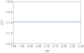
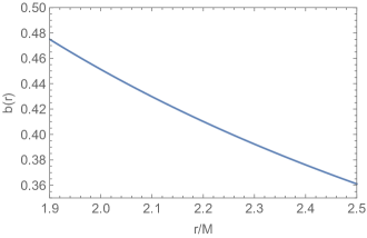
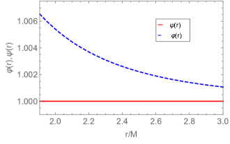
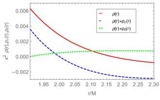
Figure 1: Solutions for the metric fields $\zeta(r)$ and $b(r)$, the scalar fields $\varphi(r)$ and $\psi(r)$, and the matter fields $\rho$, $p_{r}$ and $p_{t}$, where for the latter two it is displayed the combination of fields that bear directly to the NEC, i.e., $\rho+p_{r}$ and $\rho+p_{t}$. The values for the parameters are $\zeta_{0}=-10.96$, $M=1$, the throat radius is at $r_{0}=2\sqrt{10/11}=1.90693$, $\psi_{0}=1$, $\psi_{1}=0$, and $V_{0}=-42$. Both the scalar fields are finite for all $r$ and converge to the same constant at infinity, which implies $\varphi-\psi\to 0$ at infinity. Relative to the NEC, note that $\rho+p_{r}$ is positive at $r=r_{0}$ and changes sign at a finite value of $r$, $r=2$, and $\rho+p_{t}$ is positive for every value of $r$. Note that $\rho$ is also positive at $r=r_{0}$ and changes sign at a higher value of $r$, $r=2.16$, after which the WEC is violated. Thus, the NEC and WEC are satisfied at the wormhole throat but are violated somewhere further up. In order to maintain the validity of the NEC we have to cut it before it starts to be violated and match it to an exterior vacuum. See the text for more details.

Here we are interested in finding solutions that do not violate the matter NEC anywhere, Eqs. (24)-(25), in particular at the throat, $\rho\left(r_{0}\right)+p_{r}\left(r_{0}\right)>0$ and $\rho\left(r_{0}\right)+p_{t}\left(r_{0}\right)>0$, and possibly at its neighborhood. As we will see, a solution that respects these conditions is obtained for $\alpha=\gamma=\delta=0$, and $\beta=1$. For these choices, Eqs. (29) and (30) yield

$$\zeta\left(r\right)=\zeta_{0}\,,$$ (32)

$$b\left(r\right)=\frac{r_{0}^{2}}{r}\,,$$ (33)

respectively. Thus, the line element Eq. (15) can be written for the interior wormhole region containing the throat as

$$ds^{2}=-e^{\zeta_{0}}dt^{2}+\left[1-\frac{r_{0}^{2}}{r^{2}}\right]^{-1}dr^{2}+r^{2}\left(d\theta^{2}+\sin^{2}\theta d\phi^{2}\right)\,.$$ (34)

Choosing $\eta=2$ Eq. (31) yields

$$V\left(\varphi,\psi\right)=V_{0}\left(\varphi-\psi\right)^{2}\,.$$ (35)

Inserting the metric solutions, Eqs. (32) and (33), into Eqs. (22) and (III.1) gives

$$r_{0}^{2}+r^{4}V_{0}\left(\varphi-\psi\right)=0\,,$$ (36)

and

$$\psi^{\prime\prime}-\frac{\psi^{\prime 2}}{2\psi}+\frac{\psi^{\prime}}{r}\left[\frac{2-\left(\frac{r_{0}}{r}\right)^{2}}{1-\left(\frac{r_{0}}{r}\right)^{2}}\right]=0\,,$$ (37)

respectively. Equation (37) can be solved analytically to obtain an expression for the scalar field $\psi\left(r\right)$, namely, $\psi\left(r\right)=\left[\sqrt{\psi_{0}}+\sqrt{\psi_{1}}\arctan\left(\sqrt{\frac{r^{2}}{r_{0}^{2}}-1}\right)\right]^{2}$, where $\psi_{0}$ and $\psi_{1}$ are integrating constants. Putting it into Eq. (36) we find the solution for $\varphi\left(r\right)$. Thus, the solutions for $\varphi\left(r\right)$ and $\psi\left(r\right)$ are

$$\varphi\left(r\right)=\left[\sqrt{\psi_{0}}+\sqrt{\psi_{1}}\arctan\left(\sqrt{\frac{r^{2}}{r_{0}^{2}}-1}\right)\right]^{2}-\frac{r_{0}^{2}}{r^{4}V_{0}}.$$ (38)

and

$$\psi\left(r\right)=\left[\sqrt{\psi_{0}}+\sqrt{\psi_{1}}\arctan\left(\sqrt{\frac{r^{2}}{r_{0}^{2}}-1}\right)\right]^{2}\,,$$ (39)

respectively. We can simplify further and still find nontrivial solutions. Let us choose $\psi_{1}=0$, so that the solution for $\varphi(r)$ in Eq. (38) is

$$\varphi(r)=\psi_{0}-\frac{r_{0}^{2}}{r^{4}V_{0}}\,,$$ (40)

and the solution for $\psi(r)$ in Eq. (39) is

$$\psi(r)=\psi_{0}\,.$$ (41)

From Eqs. (40) and (41) we see that both scalar fields are finite for $r$ at the throat $r_{0}$, and for values of $r$ in its vicinity, and indeed for all $r$.

So far we have the solution for the fundamental gravitational fields, displayed in Eqs. (32) and (33) or in the line element Eq. (34), for the scalar potential, Eqs. (35), and for the fundamental extra gravitational fields represented by the scalar fields, Eqs. (40) and (41). We can now find the matter fields and study in which cases they obey the matter NEC. Inserting these solutions into Eq. (III.1), (III.1), and (21), we obtain the energy density, the radial pressure, and the tangential pressure as

$$\rho=\frac{r_{0}^{2}}{2r^{6}V_{0}\kappa^{2}}\left(24-31\frac{r_{0}^{2}}{r^{2}}\right)\,,$$ (42)

$$p_{r}=\frac{r_{0}^{2}}{2r^{6}V_{0}\kappa^{2}}\left(16-13\frac{r_{0}^{2}}{r^{2}}\right)\,,$$ (43)

$$p_{t}=\frac{r_{0}^{2}}{2r^{6}V_{0}\kappa^{2}}\left(-32+39\frac{r_{0}^{2}}{r^{2}}\right)\,,$$ (44)

respectively.

It is more useful to combine $\rho$ with $p_{r}$ and $p_{t}$ to obtain expressions directly connected to the NEC. These combinations give

$$\rho+p_{r}=\frac{2r_{0}^{2}}{r^{6}V_{0}\kappa^{2}}\left(10-11\frac{r_{0}^{2}}{r^{2}}\right),$$ (45)

$$\rho+p_{t}=\frac{4r_{0}^{2}}{r^{6}V_{0}\kappa^{2}}\left(-1+\frac{r_{0}^{2}}{r^{2}}\right).$$ (46)

At the throat, $r=r_{0}$, one has $\rho+p_{r}=\frac{2}{r_{0}^{4}(-V_{0})\kappa^{2}}$. As we want to preserve the NEC at the throat we have to set $V_{0}$ negative,

$$V_{0}<0\,.$$ (47)

In this case the NEC is valid in the throat’s neighborhood up to to the radius $r$ given by $r=\sqrt{\frac{11}{10}}\,r_{0}$. The quantity $\rho+p_{t}$ is positive for every value of $r$ and zero at the throat $r_{0}$. Thus the quantity $\rho+p_{r}$ sets the violation of the NEC. We then impose that the interior solution is valid within the following range of $r$,

$$r\leq\sqrt{\frac{11}{10}}\,r_{0}\,.$$ (48)

So, the interior solution must stop at most at $r=\sqrt{\frac{11}{10}}\,r_{0}$. Since $\rho=\frac{r_{0}^{2}}{2r^{6}V_{0}\kappa^{2}}\left(24-31\frac{r_{0}^{2}}{r^{2}}\right)$, see Eq. (42), we have that in this range of $r$ the WEC, i.e., $\rho\geq 0$, is also obeyed.

The interior solution with its metric fields $\zeta(r)$ and $b(r)$, scalar fields $\varphi(r)$ and $\psi(r)$, and matter fields $\rho$, $\rho+p_{r}$, and $\rho+p_{t}$ are displayed for all $r$ in Fig. 1 for adjusted values of the free parameters. The quantity $\rho+p_{r}$ turns negative at $r/M=2$ which is precisely $\sqrt{\frac{11}{10}}\,r_{0}$ for $r_{0}/M=2\sqrt{\frac{10}{11}}=1.90693$. The interior solution should at most stop there.

IV.1.2 Solutions outside the throat’s neighborhood up to infinity: Schwarzschild spacetimes with a cosmological constant

To guarantee that the complete solution does obey the NEC for any value of $r$, we need to match at some $r_{\Sigma}$, say, less than $\sqrt{\frac{11}{10}}\,r_{0}$ the interior solution just found to an external vacuum spherically symmetric solution. To do so, one has to derive a vacuum and asymptotically flat exterior solution, and then use the junction conditions of this theory to perform the matching with some thin shell at the boundary between the interior and exterior. Having performed this, we still have to ensure that the matter of this thin shell obeys the matter NEC, in order that the complete spacetime obeys theis condition.

We now find an exterior vacuum solution so that we can use the junction conditions to match the interior wormhole solution to the exterior vacuum solution. To do so, we put the stress-energy tensor to zero, $T_{ab}=0$, as we want a vacuum solution. In addition, we chose the scalar fields to be constant in this exterior solution, i.e., $\varphi\left(r\right)=\varphi_{e}$ and $\psi\left(r\right)=\psi_{e}$ with $\varphi_{e}$ and $\psi_{e}$ constants, $\varphi_{e}\neq\psi_{e}$, and where the subscript $e$ stands for exterior. For continuity we choose the potential to be $V=V_{0}\left(\varphi_{e}-\psi_{e}\right)^{2}$. Note that from Eq. (9) it can be seen that choosing a particular form of the potential $V$ we are also setting a particular solution for the function $f$. This means that both the interior and the exterior spacetimes must be solutions of the field equations with the same form of the potential $V$, because otherwise they would not be solutions of the same form of the function $f\left(R,\mathcal{R}\right)$. These choices imply that the field equation Eq. (12) can be written as

$$G_{ab}+\frac{V_{0}}{2}\left(\varphi_{e}-\psi_{e}\right)g_{ab}=0\,.$$ (49)

Considering that in the second term the multiplicative factors of the metric $g_{ab}$ are constant, we see that the field equation is of the same form as the Einstein field equations in vacuum with a cosmological constant given by $\frac{V_{0}}{2}\left(\varphi_{e}-\psi_{e}\right)$. Thus, the Schwarzschild solution with a cosmological constant of general relativity is a vacuum solution of the generalized hybrid theory we are studying. This class of solutions is also known as the Kottler solution, as well as Schwarzschild-dS solution if the constant cosmological term is positive and Schwarzschild–AdS solution if the constant cosmological term is negative. The metric fields $\zeta(r)$ and $b(r)$ for the exterior region outside some radius $r_{\Sigma}$ are then

$$e^{\zeta(r)}=\left(1-\frac{2M}{r}-\frac{V_{0}\left(\varphi_{e}-\psi_{e}\right)r^{2}}{6}\right)e^{\zeta_{e}}\,,$$ (50)

$$b\left(r\right)=2M+\frac{V_{0}\left(\varphi_{e}-\psi_{e}\right)r^{3}}{6}\,,$$ (51)

respectively. where $M$ is a constant of integration and represents the mass, and the factor $e^{\zeta_{e}}$ is a useful constant. The line element of the generalized field equations given by Eq. (12) in the case where the scalar fields are constant is then

$$ds^{2}= -\left({1-\frac{2M}{r}-\frac{V_{0}\left(\varphi_{e}-\psi_{e}\right)r^{2}}{6}}\right)e^{\zeta_{e}}dt^{2}+$$

$$+\left(1-\frac{2M}{r}-\frac{V_{0}\left(\varphi_{e}-\psi_{e}\right)r^{2}}{6}\right)^{-1}dr^{2}+r^{2}d\Omega^{2}\,,$$

$$r>r_{\Sigma}\,,$$

The sign of the term $\frac{V_{0}}{2}\left(\varphi_{e}-\psi_{e}\right)$ will determine whether the solution is Schwarzschild-dS or Schwarzschild-AdS. This sign will be determined by the matching surface and the imposition that the NEC holds everywhere. Wormholes in dS and AdS spacetimes in general relativity were treated in lemoslobooliveira .

To complete, the potential, scalar fields, and matter fields have then for the outer solution the following expressions,

$$V=V_{0}\left(\varphi_{e}-\psi_{e}\right)^{2}\,,$$ (53)

$$\varphi\left(r\right)=\varphi_{e}\,,$$ (54)

$$\psi\left(r\right)=\psi_{e}\,,$$ (55)

with $\varphi_{e}$ and $\psi_{e}$ constants, and

$$\rho(r)=0\,,\quad p_{r}(r)=0\,,\quad p_{t}(r)=0\,,$$ (56)

respectively.

IV.1.3 The shell at the junction: the surface density and pressure of the thin shell

To match the interior to the exterior solution we need the junction conditions for the generalized hybrid metric-Palatini gravity. The deduction of the junction equations has been performed in rosalemos1 . There are seven junction conditions in this theory that must be respected in order to perform the matching between the interior and exterior solutions, two of them that imply the existence of a thin shell of matter at the junction radius $r_{\Sigma}$. These conditions are

$$\left[h_{\alpha\beta}\right]=0\,,$$ (57)

$$\left[\varphi\right]=0\,,$$ (58)

$$\left[\psi\right]=0\,,$$ (59)

$$n^{a}\left[\partial_{a}\psi\right]=0\,,$$ (60)

$$n^{a}\left[\partial_{a}\varphi\right]=\frac{\kappa^{2}}{3}S\,,$$ (61)

$$S_{\alpha}^{\beta}-\frac{1}{3}\delta_{\alpha}^{\beta}S=-\frac{\left(\varphi_{\Sigma}-\psi_{\Sigma}\right)}{\kappa^{2}}\left[K_{\alpha}^{\beta}\right]\,,$$ (62)

$$\left[K\right]=0\,,$$ (63)

where $h_{\alpha\beta}$ is the induced metric at the junction hypersurface $\Sigma$, with Greek indexes standing for $0$ and $2,3$, the brackets $\left[X\right]$ denote the jump of any quantity $X$ across $\Sigma$, $n^{a}$ is the unit normal vector to $\Sigma$, $K=K_{\alpha}^{\alpha}$ is the trace of the extrinsic curvature $K_{\alpha\beta}$ of the surface $\Sigma$ (see, e.g., Visser:1995cc ), $S=S_{\alpha}^{\alpha}$ is the trace of the stress-energy tensor $S_{\alpha\beta}$ of the thin shell, $\delta_{\alpha}^{\beta}$ is the Kronecker delta, and the subscripts $\Sigma$ indicate the value computed at the hypersurface.

Now, the matter NEC given in Eqs. (24)-(25) should also apply to the shell, since we want this condition to be valid throughout the whole spacetime. When applied for the particular case of the thin shell the matter NEC is

$$\sigma+p\geq 0\,.$$ (64)

We have now to construct the shell out of the conditions Eqs. (57)-(64).

The condition Eq. (57) gives, on using Eqs. (32) and (50), that we can choose

$$e^{\zeta_{e}}=\frac{e^{\zeta_{0}}}{1-\frac{2M}{r_{\Sigma}}-\frac{V_{0}\left(\varphi_{e}-\psi_{e}\right)r_{\Sigma}^{2}}{6}}.$$ (65)

This factor $e^{\zeta_{e}}$ has been chosen so that the time coordinate $t$ for the interior, Eq. (34), is the same as the coordinate $t$ for the exterior, Eq. (IV.1.2). The angular part of the metrics Eq. (34) and Eq. (IV.1.2) are continuous. So the line element at the surface $\Sigma$ and outside it is

$$ds^{2}= -\left(\frac{1-\frac{2M}{r}-\frac{V_{0}\left(\varphi_{e}-\psi_{e}\right)r^{2}}{6}}{1-\frac{2M}{r_{\Sigma}}-\frac{V_{0}\left(\varphi_{e}-\psi_{e}\right)r_{\Sigma}^{2}}{6}}\right)e^{\zeta_{0}}dt^{2}+$$ (67)

$$+\left(1-\frac{2M}{r}-\frac{V_{0}\left(\varphi_{e}-\psi_{e}\right)r^{2}}{6}\right)^{-1}dr^{2}+r^{2}d\Omega^{2}\,,$$

$$r\geq r_{\Sigma}\,,$$

where we are using that the $\varphi$ and $\psi$ are continous at the matching, see below.

The condition Eq. (58) means that

$$\varphi_{e}=\varphi_{\Sigma}=\psi_{0}-\frac{r_{0}^{2}}{r_{\Sigma}^{4}V_{0}}\,,$$ (68)

where we have used Eq. (40). Whenever it occurs we keep the notation $\varphi_{e}$.

The condition Eq. (59) means that

$$\psi_{e}=\psi_{\Sigma}=\psi_{0}\,.$$ (69)

where we have used Eq. (41). Whenever it occurs we keep the notation $\psi_{e}$.

The condition Eq. (60) is empty, since $\psi$ is constant everywhere.

The condition Eq. (61) gives $\partial_{r}\varphi|_{\Sigma}=-\frac{\kappa^{2}}{3}S$, $n^{a}\partial_{a}\varphi_{e}=0$, and so, $n^{a}\left[\partial_{a}\varphi\right]=-\partial_{r}\varphi|_{\Sigma}$. All the contribution comes from the interior. Thus, Eq. (61) yields finally

$$\frac{4r_{0}^{2}}{r_{\Sigma}^{5}V_{0}}=-\frac{\kappa^{2}}{3}S\,.$$ (70)

The condition Eq. (62) can be used to detemine the surface energy density $\sigma$ and the surface transverse pressure $p$. Note that $\sigma$ is given by $S_{0}^{0}=-\sigma$ and $p$ is given by $S_{1}^{1}=S_{2}^{2}=p$. Then, from Eq. (62) we have $\sigma=\frac{1}{\kappa^{2}}\left(\varphi_{\Sigma}-\psi_{\Sigma}\right)\left[K_{0}^{0}\right]-\frac{1}{3}S$, and $p=-\frac{1}{\kappa^{2}}\left(\varphi_{\Sigma}-\psi_{\Sigma}\right)\left[K_{0}^{0}\right]+\frac{1}{3}S$. For the interior solution given in Eq. (34) and the exterior solution given in Eq. (IV.1.2) we can compute $\left[K_{0}^{0}\right]$, $\left[K_{0}^{0}\right]=\frac{r_{0}\zeta_{0}}{2r_{\Sigma}^{2}}\sqrt{1-\frac{r_{0}^{2}}{r_{\Sigma}^{2}}}-\frac{r_{\Sigma}^{3}V_{0}\left(\varphi_{e}-\psi_{e}\right)-6M}{6r_{\Sigma}^{2}\sqrt{1-\frac{2M}{r_{\Sigma}}-\frac{r_{\Sigma}^{2}}{6}V_{0}\left(\varphi_{e}-\psi_{e}\right)}}$, which upon using Eq. (68), (69), and (70) gives

$$\left[K_{0}^{0}\right]=\frac{r_{0}\zeta_{0}}{2r_{\Sigma}^{2}}\sqrt{1-\frac{r_{0}^{2}}{r_{\Sigma}^{2}}}+\frac{\frac{r_{0}^{2}}{r_{\Sigma}}-6M}{6r_{\Sigma}^{2}\sqrt{1-\frac{2M}{r_{\Sigma}}+\frac{r_{0}^{2}}{6r_{\Sigma}^{2}}}}\,.$$ (71)

Then, $\sigma$ and $p$ are given by

$$\sigma=\frac{4r_{0}^{2}}{\kappa^{2}V_{0}r_{\Sigma}^{5}}\left(1-\frac{1}{4}\,r_{\Sigma}\left[K_{0}^{0}\right]\right)\,,$$ (72)

$$p=-\frac{4r_{0}^{2}}{\kappa^{2}V_{0}r_{\Sigma}^{5}}\left(1+\frac{1}{8}\,r_{\Sigma}\left[K_{0}^{0}\right]\right)\,,$$ (73)

respectively.

The condition Eq. (63) means that the matching has to be performed at the radius $r_{\Sigma}$ such that the jump in the trace of the extrinsic curvature is zero, i.e., $\left[K\right]=\frac{1}{r_{\Sigma}}\left[\frac{r_{0}\zeta_{0}}{2r_{\Sigma}}\sqrt{1-\left(\frac{r_{0}}{r_{\Sigma}}\right)^{2}}-\sqrt{1-\left(\frac{r_{0}}{r_{\Sigma}}\right)^{4}}-\sqrt{1-\left(\frac{r_{0}}{r_{\Sigma}}\right)^{5}}+\right.$

$\left.\frac{2-\frac{3M}{r_{\Sigma}}-\frac{1}{2}r_{\Sigma}^{2}V_{0}\left(\varphi_{e}-\psi_{e}\right)}{\sqrt{1-\frac{2M}{r_{\Sigma}}-\frac{1}{6}r_{\Sigma}^{2}V_{0}\left(\varphi_{e}-\psi_{e}\right)}}\right]=0$. Upon using Eqs. (68), (69), and (70) it gives

$$\left[K\right]=\frac{1}{r_{\Sigma}}\left[\frac{r_{0}\zeta_{0}}{2r_{\Sigma}}\sqrt{1-\left(\frac{r_{0}}{r_{\Sigma}}\right)^{2}}-\sqrt{1-\left(\frac{r_{0}}{r_{\Sigma}}\right)^{4}}\right.$$

$$\left.-\sqrt{1-\left(\frac{r_{0}}{r_{\Sigma}}\right)^{5}}+\frac{2-\frac{3M}{r_{\Sigma}}+\frac{r_{0}^{2}}{2r_{\Sigma}^{2}}}{\sqrt{1-\frac{2M}{r_{\Sigma}}+\frac{r_{0}^{2}}{6r_{\Sigma}^{2}}}}\right]=0\,.$$ (74)

The condition Eq. (64) is the matter NEC that should be valid on the shell. In this way we can keep the validity of the matter NEC throughout the whole spacetime. The relevant quantity is $\sigma+p$. Using Eqs. (72) and  (73) we find

$$\sigma+p=-\frac{3r_{0}^{2}}{2\kappa^{2}V_{0}r_{\Sigma}^{4}}\left[K_{0}^{0}\right]\,.$$ (75)

Finding a combination of parameters that fulfills all the junction conditions, plus the matter NEC everywhere, is a problem that requires some fine-tuning. We now turn to this.

IV.2 The full wormhole solution obeying the matter null energy condition everywhere

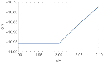
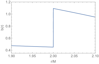
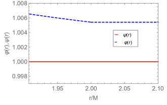
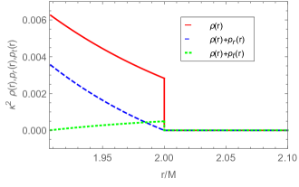
Figure 2: Full wormhole solution from the throat to infinity with the NEC and WEC being obeyed everywhere. The solutions are for the metric fields $\zeta(r)$ and $b(r)$, the scalar fields $\varphi(r)$ and $\psi(r)$, and the matter fields $\rho$, $\rho+p_{r}$ and $\rho+p_{t}$. The values of the free parameters are $\zeta_{0}=-10.96$, $M=1$, the throat is at $r_{0}=2\sqrt{10/11}=1.907$, $\psi_{0}=1$, $\psi_{1}=0$, $V_{0}=-42$, and the matching surface is at $r_{\Sigma}=2$. The metric fields $\zeta(r)$ and $b(r)$ are asymptotically AdS, and a thin shell of matter is perceptibly present at the matching surface $r_{\Sigma}=2$ (more properly at $r_{\Sigma}=2M$ in our solution, and here we put $M=1$), thus outside the gravitational radius of the solution. Both the scalar fields are finite for all $r$ and converge to the same constant at infinity, which implies $\varphi-\psi\to 0$ at infinity. Relative to the NEC, note that $\rho+p_{r}$ is positive at $r=r_{0}$ and up to $r=2$ and for $r>2$ is zero. The quantity $\rho+p_{t}$ is zero at $r=r_{0}$, positive for every other value of $r<2$, and for $r>2$ is zero. At the shell $r=2$ one has $\kappa^{2}(\sigma+p)=\frac{0.02}{(-V_{0})}=0.0005$ (not displayed). Thus the NEC is satisfied everywhere. See the text for more details.

First, the solution scales with the exterior mass $M$ appearing in Eq. (IV.1.2) and so all quantities can be normalized to it.

Second, the parameter $V_{0}$, as we already argued, must be negative, $V_{0}<0$, so that the NEC is verified at the throat and its vicinity, see Eq. (45). In this case the WEC is also verified at the throat and its vicinity.

Third, the junction condition $\left[K\right]=0$, see Eq. (IV.1.3), can be achieved only for certain values of the radius $r\equiv r_{\Sigma}$. We certainly need to guarantee that the radius $r_{\Sigma}$ at which $\left[K\right]=0$ happens is inside the region $r<\sqrt{11/10}\,r_{0}$, see Eq. (48), so that the interior solution does not violate the NEC. Manipulation of the parameters of the interior solution shows that these conditions can be achieved by changing the parameter $r_{0}$.

Fourth, once we have set values for $r_{0}$ and $r_{\Sigma}$, Eq. (IV.1.3) automatically sets the value of the parameter $\zeta_{0}$ and hence, Eq. (71) sets the value of $\left[K_{0}^{0}\right]$. Then, by Eqs. (72) and (73), we see that choosing a value of the parameter $V_{0}$ determines the values of $\sigma$ and $p$. However, since we already argued that $V_{0}$ must be negative in order for the NEC to be verified at the throat, see Eq. (45), then the signs of $\sigma$ and $p$ are determined even without specifying an exact value for $V_{0}$. Moreover, since $V_{0}<0$, the NEC at the shell, Eq. (75), is satisfied if $\left[K_{0}^{0}\right]\geq 0$.

Fifth, having all the parameters determined, one has in general to verify that $r_{\Sigma}$ is greater that the gravitational radius $r_{g}$ of the solution. If this were not the case then there would be a horizon and the solution would be invalid. In our solution, one has $r_{g}=2M\left[1+2V_{0}(\varphi_{e}-\psi_{e})M^{2}/3\right]$, see Eq. (IV.1.2). However, using Eqs. (68) and (69), one can write the gravitational radius as $r_{g}=2M\left(1-\frac{2M^{2}r_{0}^{2}}{3r_{\Sigma}^{4}}\right)$, which is smaller than $r_{\Sigma}$ for any value of $r_{\Sigma}$ between $r_{0}$ and $\sqrt{\frac{11}{10}}r_{0}$. This implies that in the range of solutions that we are interested in this step is automatically satisfied.

We are now in a position to specify a set of parameters for which the matter NEC is obeyed everywhere, i.e., in the interior, on the shell, and in the exterior, the latter being a trivial case since there is no matter in this region. We give an example and consider a wormhole with mass $M$. Note that the conclusions are the same for any combination of $r_{0}$ and $r_{\Sigma}$ within the allowed region for these two parameters. A concrete convenient example is to have a wormhole interior region for which the radius $r_{0}$ of the throat has the value $r_{0}=\sqrt{\frac{10}{11}}2M$. Then, from Eq. (48) we can put $r_{\Sigma}=2M$ and have the matter NEC in the interior being obeyed. With these values of $r_{0}$ and $r_{\Sigma}$, Eq. (IV.1.3) sets the value of $\zeta_{0}$ to be $\zeta_{0}=-10.96$. From Eq. (71) we get $\left[K_{0}^{0}\right]=0.049$, and using Eqs. (72) and (73) we compute the values of the stress-energy tensor at the shell, which become $\kappa^{2}\sigma=\frac{0.44}{V_{0}}$ and $\kappa^{2}p=-\frac{0.46}{V_{0}}$, respectively, and hence $\kappa^{2}\left(\sigma+p\right)=-\frac{0.02}{V_{0}}$. Since $V_{0}<0$ we see that $\sigma+p>0$ and thus the NEC is satisfied at the shell. Since $\kappa^{2}\sigma=\frac{0.44}{V_{0}}$ and $V_{0}<0$ we have $\sigma<0$. So the WEC does not hold on the shell but holds everywhere else. The NEC holds everywhere.

This completes our full wormhole solution. Fig. 2 displays a solution with $M=1$, $r_{0}=\sqrt{\frac{10}{11}}2$, $r_{\Sigma}=2$, $\zeta_{0}=-10.96$, $V_{0}=-42$. This wormhole solution obeys the matter NEC everywhere in conformity with our aim.

Other wormhole solutions in this generalized hybrid theory with other choices of parameters, within the ranges stated above, that obey the matter NEC everywhere can be found along the lines we have presented.

V Conclusion

In this work, we found traversable asymptotically AdS wormhole solutions that obey the NEC everywhere in the generalized hybrid metric-Palatini gravity theory, so there is no need for exotic matter. The generalized hybrid theory consists in a gravitational action given by $f\left(R,\cal{R}\right)$, where $R$ is the metric Ricci scalar, and $\mathcal{R}\equiv\mathcal{R}^{ab}g_{ab}$ is the Palatini curvature defined in terms of an independent connection, to which a matter action is added. The gravitational action can be given in the scalar-tensor representation where the metric Ricci scalar $R$ is still present but now coupled to two scalar fields $\varphi$ and $\psi$. The equations of motion in this representation were obtained.

The interior wormhole solution obtained verifies the NEC near and at the throat of the wormhole. The matching of the interior solution to an exterior vacuum solution yields a thin shell respecting also the NEC. Finding a combination of parameters that allow for the interior and the exterior solution to be matched without violating the NEC in the interior solution and at the thin shell is a problem that requires fine-tuning, but can be acomplished. We presented a specific combination of parameters with which it is possible to build the full wormhole solution and found that it is asymptotically AdS. Most of the work that has been done in hybrid metric-Palatini gravity theories has been aimed to find solutions where the NEC is satisfied solely at the throat of the wormhole. Within these theories our solution is the first where the NEC is verified for the entire spacetime.

There are two main interesting conclusions. On one hand, the existence of these solutions is in agreement with the understanding that traversable wormholes supported by extra fundamental gravitational fields, here in the guise of scalar fields, can occur without the need of exotic matter. On the other hand, the rather contrived construction necessary to build a spacetime complete wormhole solution may indicate that there are not many such solutions around in this class of theories.

- (1) M. S. Morris and K. S. Thorne, “Wormholes in space-time and their use for interstellar travel: A tool for teaching general relativity”, Am. J. Phys. 56, 395 (1988).
- (2) M. Visser, Lorentzian wormholes: From Einstein to Hawking (Springer-Verlag, New York, 1996).
- (3) J. P. S. Lemos, F. S. N. Lobo, and S. Q. Oliveira, “Morris-Thorne wormholes with a cosmological constant”, Phys. Rev. D 68, 064004 (2003); arXiv:gr-qc/0302049.
- (4) A. G. Agnese and M. La Camera, “Wormholes in the Brans-Dicke theory of gravitation”, Phys. Rev. D 51, 2011 (1995).
- (5) K. K. Nandi, B. Bhattacharjee, S. M. K. Alam, and J. Evans, “Brans-Dicke wormholes in the Jordan and Einstein frames”, Phys. Rev. D 57, 823 (1998); arXiv:0906.0181 [gr-qc].
- (6) K. A. Bronnikov and S. W. Kim, “Possible wormholes in a brane world”, Phys. Rev. D 67, 064027 (2003); arXiv:gr-qc/0212112.
- (7) M. La Camera, “Wormhole solutions in the Randall-Sundrum scenario”, Phys. Lett. B 573, 27 (2003); arXiv:gr-qc/0306017.
- (8) F. S. N. Lobo, “Exotic solutions in general relativity: Traversable wormholes and ‘warp drive’ spacetimes”, in Classical and Quantum Gravity Research, editors M. N. Christiansen and T. K. Rasmussen (Nova Science Publishers, 2008), p. 1; arXiv:0710.4474 [gr-qc].
- (9) R. Garattini and F. S. N. Lobo, “Self sustained phantom wormholes in semi-classical gravity”, Classical Quantum Gravity 24, 2401 (2007); arXiv:gr-qc/0701020.
- (10) F. S. N. Lobo, “General class of wormhole geometries in conformal Weyl gravity”, Classical Quantum Gravity 25, 175006 (2008); arXiv:0801.4401 [gr-qc].
- (11) R. Garattini and F. S. N. Lobo, “Self-sustained traversable wormholes in noncommutative geometry”, Phys. Lett. B 671, 146 (2009); arXiv:0811.0919 [gr-qc].
- (12) F. S. N. Lobo and M. A. Oliveira, “General class of vacuum Brans-Dicke wormholes”, Phys. Rev. D 81, 067501 (2010); arXiv:1001.0995 [gr-qc].
- (13) R. Garattini and F. S. N. Lobo, “Self-sustained wormholes in modified dispersion relations”, Phys. Rev. D 85, 024043 (2012); arXiv:1111.5729 [gr-qc].
- (14) F. S. N. Lobo (editor), Wormholes, Warp Drives and Energy Conditions, Fundam. Theor. Phys. 189, (Springer International Publishing, 2017).
- (15) F. S. N. Lobo and M. A. Oliveira, “Wormhole geometries in modified theories of gravity”, Phys. Rev. D 80, 104012 (2009); arXiv:0909.5539 [gr-qc].
- (16) N. M. Garcia and F. S. N. Lobo, “Wormhole geometries supported by a nonminimal curvature-matter coupling”, Phys. Rev. D 82, 104018 (2010); arXiv:1007.3040 [gr-qc].
- (17) N. Montelongo Garcia and F. S. N. Lobo, “Nonminimal curvature-matter coupled wormholes with matter satisfying the null energy condition”, Class. Quant. Grav. 28, 085018 (2011); arXiv:1012.2443 [gr-qc].
- (18) T. Harko, F. S. N. Lobo, M. K. Mak, and S. V. Sushkov, “Modified-gravity wormholes without exotic matter”, Phys. Rev. D 87, 067504 (2013); arXiv:1301.6878 [gr-qc].
- (19) B. Bhawal and S. Kar, “Lorentzian wormholes in Einstein–Gauss-Bonnet theory”, Phys. Rev. D 46, 2464 (1992).
- (20) G. Dotti, J. Oliva, and R. Troncoso, “Exact solutions for the Einstein-Gauss-Bonnet theory in five dimensions: Black holes, wormholes and spacetime horns”, Phys. Rev. D 75, 024002 (2007); arXiv:0706.1830 [hep-th].
- (21) M. R. Mehdizadeh, M. Kord Zangeneh, and F. S. N. Lobo, “Einstein-Gauss-Bonnet traversable wormholes satisfying the weak energy condition”, Phys. Rev. D 91, no. 8, 084004 (2015); arXiv:1501.04773 [gr-qc].
- (22) F. S. N. Lobo, “A general class of braneworld wormholes”, Phys. Rev. D 75, 064027 (2007); arXiv:gr-qc/0701133.
- (23) L. A. Anchordoqui, S. E. Perez Bergliaffa, and D. F. Torres, “Brans-Dicke wormholes in nonvacuum spacetime”, Phys. Rev. D 55, 5226 (1997); arXiv:gr-qc/9610070.
- (24) S. Capozziello, T. Harko, T. S. Koivisto, F. S. N. Lobo, and G. J. Olmo, “Wormholes supported by hybrid metric-Palatini gravity”, Phys. Rev. D 86, 127504 (2012) [arXiv:1209.5862 [gr-qc]].
- (25) T. Harko, T. S. Koivisto, F. S. N. Lobo, and G. J. Olmo, “Metric-Palatini gravity unifying local constraints and late-time cosmic acceleration”, Phys. Rev. D 85, 084016 (2012); arXiv:1110.1049 [gr-qc].
- (26) G. J. Olmo, “Palatini approach to modified gravity: theories and beyond”, Int. J. Mod. Phys. D 20, 413 (2011); arXiv:1101.3864 [gr-qc].
- (27) S. Capozziello, T. Harko, T. S. Koivisto, F. S. N. Lobo, and G. J. Olmo, “Cosmology of hybrid metric-Palatini f(X)-gravity”, J. Cosmol. Astropart. Phys. (JCAP) 04 (2013) 011; arXiv:1209.2895 [gr-qc].
- (28) S. Capozziello, T. Harko, T. S. Koivisto, F. S. N. Lobo, and G. J. Olmo, “The virial theorem and the dark matter problem in hybrid metric-Palatini gravity”, J. Cosmol. Astropart. Phys. (JCAP) 07 (2013) 024; arXiv:1212.5817 [physics.gen-ph].
- (29) S. Capozziello, T. Harko, T. S. Koivisto, F. S. N. Lobo, and G. J. Olmo, “Galactic rotation curves in hybrid metric-Palatini gravity”, Astropart. Phys. 50-52, 65 (2013); arXiv:1307.0752 [gr-qc].
- (30) S. Capozziello, T. Harko, F. S. N. Lobo, and G. J. Olmo, “Hybrid modified gravity unifying local tests, galactic dynamics and late-time cosmic acceleration”, Int. J. Mod. Phys. D 22, 1342006 (2013); arXiv:1305.3756 [gr-qc].
- (31) S. Capozziello, T. Harko, T. S. Koivisto, F. S. N. Lobo, and G. J. Olmo, “Hybrid metric-Palatini gravity”, Universe 1, 199 (2015); arXiv:1508.04641 [gr-qc].
- (32) T. Harko, F. S. N. Lobo. Extensions of Gravity: Curvature-Matter Couplings and Hybrid Metric-Palatini Gravity (Cambridge Monographs on Mathematical Physics). Cambridge: Cambridge University Press (2018).
- (33) N. Tamanini and C. G. Boehmer, “Generalized hybrid metric-Palatini gravity”, Phys. Rev. D 87, 084031 (2013); arXiv:1302.2355 [gr-qc].
- (34) J. L. Rosa, S. Carloni, J. P. S. Lemos, and F. S. N. Lobo, “Cosmological solutions in generalized hybrid metric-Palatini gravity”, Phys. Rev. D 95, 124035 (2017); arXiv:1703.03335 [gr-qc].
- (35) J. L. Rosa and J. P. S. Lemos, “Junction conditions and thin shells in the generalized hybrid metric-Palatini gravity”, to be submitted (2018).