Resonant Di-Higgs Production at Gravitational Wave Benchmarks: A Collider Study using Machine Learning

Abstract

We perform a complementarity study of gravitational waves and colliders in the context of electroweak phase transitions choosing as our template the xSM model, which consists of the Standard Model augmented by a real scalar. We carefully analyze the gravitational wave signal at benchmark points compatible with a first order phase transition, taking into account subtle issues pertaining to the bubble wall velocity and the hydrodynamics of the plasma. In particular, we comment on the tension between requiring bubble wall velocities small enough to produce a net baryon number through the sphaleron process, and large enough to obtain appreciable gravitational wave production. For the most promising benchmark models, we study resonant di-Higgs production at the high-luminosity LHC using machine learning tools: a Gaussian process algorithm to jointly search for optimum cut thresholds and tuning hyperparameters, and a boosted decision trees algorithm to discriminate signal and background. The multivariate analysis on the collider side is able either to discover or provide strong statistical evidence of the benchmark points, opening the possibility for complementary searches for electroweak phase transitions in collider and gravitational wave experiments.

1 Introduction

Understanding the nature of the electroweak phase transition (EWPT) is a major goal in particle physics. A first order phase transition can be obtained by introducing new physics at the electroweak scale and this new physics can be explored at the high luminosity Large Hadron Collider (HL-LHC). On the other hand, a first order phase transition can generate gravitational waves that may be within the reach of future space-based detectors. It becomes important to understand how this complementarity plays out in concrete models - for example, can one obtain regions of parameter space where all conditions - first order phase transition, detectable gravitational waves, and a strong enough signal at the HL-LHC - are met?

The simplest template for studying these questions is the xSM model Profumo:2007wc ; Profumo:2014opa ; Huang:2017jws , which consists of the Standard Model (SM) extended by a real scalar. We make no comments about the completion of this model in the UV, the naturalness conflicts associated with introducing yet another scalar in addition to the Higgs, etc. Rather, our philosophy is to use the xSM as the simplest extension of the Higgs sector in which a complementary gravitational wave and collider study can be performed.

The purpose of the current paper is to first carefully explore gravitational wave signatures associated with the EWPT, and then study resonant di-Higgs production at the HL-LHC in the same context.

The new features of our study are the following:

$(i)$ While the picture of complementarity presented above is appealing, making concrete connections from gravitational wave studies to particle physics at the electroweak scale faces many technical challenges in the calculations of electroweak baryogenesis (EWBG), EWPT and gravitational waves Morrissey:2012db . While we do not intend to target all these challenges in one strike, we initiate a process of making this connection more solid by presenting a careful treatment of the gravitational wave calculations.

We address several subtle issues pertaining to the bubble wall velocity and the hydrodynamics of the plasma, in particular the tension between requiring bubble wall velocities small enough to produce a net baryon number through the sphaleron process, and large enough to obtain appreciable gravitational wave production. The velocity that enters the calculations of EWBG might not be the bubble wall velocity for plasma in the modes of deflagrations and supersonic deflagrations ahead of the bubble wall, as demonstrated by hydrodynamic analysis and simulations Espinosa:2010hh . This has the consequence that for a large wall velocity, a much smaller velocity for EWBG can be obtained and EWPT can be accompanied by a strong gravitational wave signal No:2011fi . Therefore in our analysis, we make a clear distinction between these two velocities and determine their relation from a hydrodynamic analysis of the fluid profiles.

For our benchmark models, we compute the gravitational wave energy spectra and signal-to-noise ratio for future space-based gravitational wave experiments.

$(ii)$ On the collider side, our objective is to apply the machine learning techniques initiated in Alves:2017ued to resonant di-Higgs production, at benchmark points that are compatible with acceptable EWPT and that hold out the most optimistic prospects from gravitational wave observations. We conduct a di-Higgs study at the HL-LHC: $pp\rightarrow h_{2}\rightarrow h_{1}h_{1}\rightarrow b\bar{b}\gamma\gamma$, where $h_{1}$ denotes the SM Higgs. We carefully incorporate all relevant backgrounds in our study. In particular, we are careful to include contributions coming from jets being misidentified as photons, as well as light flavor jets or $c$-jets being misidentified as $b$-jets.

We utilize two recent advances in the machine learning literature for our collider study. Firstly, recent results hyperopt show that in terms of efficiency, Bayesian hyperparameter optimization of machine learning models tends to perform better than random, grid, or manual optimization. We use the Python library Hyperopt hyperopt to optimize cuts on kinematic variables in our study. The second tool from the machine learning community that we apply is XGBoost xgb (eXtreme Gradient Boosted Decision Trees), which has become increasingly popular among Kaggle competitors and data scientists in industry, especially since its winning performance in the HEP meets ML Kaggle challenge. Unlike a simple gradient boosting classifier, where classifiers (decision trees) are added sequentially, XGBoost is able to parallelize this task, leading to superior performance. Both cut thresholds and Boosted Decision Trees (BDT) hyperparameters are jointly optimized for maximum collider sensitivity.

	$\cos\theta$	$m_{h_{2}}$	$v_{s}$	$\lambda$	$a_{1}$	$a_{2}$	$b_{3}$	$b_{4}$	$\lambda_{111}$	$\lambda_{211}$	$\frac{\lambda_{111}}{\lambda^{\text{SM}}_{111}}$	$\Gamma_{h_{2}}^{\text{tot}}$	BR($h_{1}h_{1}$)	$T_{c}$	$T_{n}$	$v_{h}(T_{n})$	$\alpha$	$\beta/H_{n}$	$v_{w}$	SNR(LISA)
		(GeV)	(GeV)		(GeV)		(GeV)		(GeV)	(GeV)		(GeV)	(%)	(GeV)	(GeV)	(GeV)			($v_{+}=0.05$)
BM5	0.984	455.	47.4	0.179	-708.	4.59	-607.	0.85	47.0	92.8	1.48	2.06	30.5	59.3	33.5	234.	1.88	127.	0.766	9133.
BM6	0.986	511.	40.7	0.185	-744.	5.11	-618.	0.82	46.9	90.5	1.48	2.44	22.8	62.3	49.7	217.	0.48	726.	0.345	20.
BM7	0.988	563.	40.5	0.188	-845.	5.82	-151.	0.08	47.3	103.0	1.49	2.90	23.2	57.3	28.4	237.	3.45	67.	0.861	6537.
BM8	0.992	604.	36.4	0.175	-900.	7.48	-424.	0.28	45.3	120.4	1.43	2.72	31.9	56.3	33.9	232.	1.92	444.	0.770	7473.
BM9	0.994	662.	32.9	0.171	-978.	9.19	-542.	0.53	44.4	133.9	1.40	2.84	35.2	54.6	34.0	230.	1.97	141.	0.774	10016.
BM10	0.993	714.	29.2	0.186	-941.	8.05	497.	0.38	45.1	108.3	1.42	3.31	18.5	61.2	52.8	205.	0.41	1307.	0.274	0.50
BM11	0.996	767.	24.5	0.167	-922.	10.35	575.	0.41	41.6	118.0	1.31	2.59	26.4	63.3	58.3	186.	0.29	2586.	0.164	0.00048
BM12	0.994	840.	21.7	0.197	-988.	8.71	356.	0.83	44.1	73.3	1.39	3.98	6.1	68.9	67.4	152.	0.13	10730.	0.078	6.48$\times 10^{-10}$

Table 1: A subset of the benchmarks used in Ref. Huang:2017jws (Table.I) that can give a strongly first order EWPT as well as satisfying all phenomenological constraints. BM1-4 are neglected for reasons explained in the text. $\lambda_{111}$ and $\lambda_{211}$ are cubic couplings, given with the convention of Ref. Profumo:2007wc ; Profumo:2014opa ; Huang:2017jws : $\lambda_{111}=i\lambda_{h_{1}h_{1}h_{1}}/6$ and $\lambda_{112}=i\lambda_{h_{1}h_{1}h_{2}}/2$. Parameters that are relevant for EWPT and gravitational waves are also tabulated for each benchmark. The last column is the signal-to-noise ratio which quantifies the gravitational wave discovery prospect at LISA. See text for more detailed explanation.

Our paper is structured as follows. In Section 2, we introduce the xSM model and settle on the benchmarks that allow a first order phase transition. In Section 3, we calculate the gravitational wave energy spectra and signal-to-noise ratio for several benchmark models. In Section 4, we perform our collider analysis. We end with our Conclusions.

2 The model

The model “xSM” constitutes one of the simplest extentions of the SM where a real scalar gauge singlet $S$ is added to the particle content. The potential for the “xSM” model is defined with the convention following Ref. Profumo:2007wc ; Profumo:2014opa ; Huang:2017jws :

$$V(H,S) = -\mu^{2}H^{\dagger}H+\lambda(H^{\dagger}H)^{2}+\frac{a_{1}}{2}H^{\dagger}HS$$ (1)

$$+\frac{a_{2}}{2}H^{\dagger}HS^{2}+\frac{b_{2}}{2}S^{2}+\frac{b_{3}}{3}S^{3}+\frac{b_{4}}{4}S^{4}.$$

Here $H^{\text{T}}=(G^{+},(v+h+iG^{0})/\sqrt{2})$ is the SM Higgs doublet and $S=v_{s}+s$ defines the real scalar singlet. All the parameters appearing here are real. The minimization conditions of this potential at the vacuum $(v,v_{s})$ allows one to eliminate $\mu,b_{2}$ by

$$\mu^{2}=\lambda v^{2}+\frac{1}{2}v_{s}(a_{1}+a_{2}v_{s}),$$

$$b_{2}=-\frac{1}{4v_{s}}[v^{2}(a_{1}+2a_{2}v_{s})+4v_{s}^{2}(b_{3}+b_{4}v_{s})].$$ (2)

With these substitutions, the mass matrix for $(h,s)$ is found to be:

$$m^{2}=\left(\begin{array}[]{cc}2\lambda v^{2}&\frac{1}{2}a_{1}v+v_{s}v\ a_{2}\\ \frac{1}{2}a_{1}v+v_{s}va_{2}&\ \ \ \ \ \ v_{s}(b_{3}+2v_{s}b_{4})-\frac{1}{4v_{s}}v^{2}a_{1}\end{array}\right),$$ (5)

which can then be diagonalized by a rotation angle $\theta$. This results in the physical scalars $(h_{1},h_{2})$ in terms of the gauge eigenstates $(h,s)$:

$$h_{1}=c_{\theta}h+s_{\theta}s,\quad\quad h_{2}=-s_{\theta}h+c_{\theta}s.$$ (6)

where $h_{1}$ is identified as the 125 GeV Higgs scalar and further $m_{h_{2}}>m_{h_{1}}$. Consequently, three of the potential parameters $(\lambda,a_{1},a_{2})$ can be replaced by three physical parameters $m_{h_{1}}$, $m_{h_{2}}$ and $\theta$:

$$\lambda=\frac{m_{h_{1}}^{2}c_{\theta}^{2}+m_{h_{2}}^{2}s_{\theta}^{2}}{2v^{2}},$$

$$a_{1}=\frac{2v_{s}}{v^{2}}[2v_{s}^{2}(2b_{4}+\tilde{b}_{3})-m_{h_{1}}^{2}-m_{h_{2}}^{2}+c_{2\theta}(m_{h_{1}}^{2}-m_{h_{2}}^{2})],$$

$$a_{2}=\frac{-1}{2v^{2}v_{s}}[-2v_{s}(m_{h_{1}}^{2}+m_{h_{2}}^{2}-4b_{4}v_{s}^{2})$$

$$\hskip 56.9055pt+(m_{h_{1}}^{2}-m_{h_{2}}^{2})(2c_{2\theta}v_{s}-vs_{2\theta})+4\tilde{b}_{3}v_{s}^{3}],$$ (7)

where $\tilde{b}_{3}\equiv b_{3}/v_{s}$. Then the full set of independent unknown parameters are

$$\centering v_{s},\quad\quad m_{h_{2}},\quad\quad\theta,\quad\quad b_{3},\quad\quad b_{4},\@add@centering$$ (8)

while keeping in mind that $v$ can be solved from the Fermi constant and $m_{h_{1}}=125\text{GeV}$. With the model parameters fully specified, the cubic scalar couplings that are relevant for di-Higgs production are $\lambda_{h_{1}h_{1}h_{1}}$ and $\lambda_{h_{2}h_{1}h_{1}}$, given by

$$i\lambda_{h_{1}h_{1}h_{1}}=6\Big{[}\lambda vc_{\theta}^{3}+\frac{1}{4}c_{\theta}^{2}s_{\theta}\left(2a_{2}v_{s}+a_{1}\right)+\frac{1}{2}a_{2}vc_{\theta}s_{\theta}^{2}$$

$$\hskip 45.52458pt+\frac{1}{3}s_{\theta}^{3}\left(3b_{4}v_{s}+b_{3}\right)\Big{]},$$

$$i\lambda_{h_{1}h_{1}h_{2}}=\frac{1}{2}\Big{[}-2c_{\theta}s_{\theta}^{2}\left(2a_{2}v_{s}+a_{1}-6b_{4}v_{s}-2b_{3}\right)$$

$$\hskip 22.76228pt+4v\left(a_{2}-3\lambda\right)c_{\theta}^{2}s_{\theta}+c_{\theta}^{3}\left(2a_{2}v_{s}+a_{1}\right)-2a_{2}vs_{\theta}^{3}\Big{]}.\ \ \ \ \$$ (9)

In the absence of mixing of the scalars when $\theta=0$, the cubic Higgs coupling reduces to its SM value $i\lambda_{h_{1}h_{1}h_{1}}=3m_{h_{1}}^{2}/v$ while $i\lambda_{h_{1}h_{1}h_{2}}$ vanishes. For small $\theta$ as suggested by experimental measurements, the following approximation is obtained for the cubic couplings through a Taylor expansion:

$$i\lambda_{h_{1}h_{1}h_{1}} = \frac{3m_{h_{1}}^{2}}{v}-\frac{3\theta^{2}}{2v}\left[4(2b_{4}+\tilde{b}_{3})v_{s}^{2}+3m_{h_{1}}^{2}-4m_{h_{2}}^{2}\right],$$

$$i\lambda_{h_{1}h_{1}h_{2}} = \theta\frac{-4(2b_{4}+\tilde{b}_{3})v_{s}^{2}-2m_{h_{1}}^{2}+3m_{h_{2}}^{2}}{v}.$$ (10)

The gauge and Yukawa couplings of $h_{1}$ are reduced by a factor $c_{\theta}$ and the couplings of $h_{2}$ are $-s_{\theta}$ times the SM values, that is,

$$\lambda_{h1XX}=c_{\theta}\lambda^{\text{SM}}_{h1XX},\quad\quad\lambda_{h2XX}=-s_{\theta}\lambda^{\text{SM}}_{h2XX},$$ (11)

where $XX$ denotes $W^{+}W^{-}$, $ZZ$ and $\bar{f}f$.

Since it modifies the Higgs couplings, the mixing angle is constrained by experiments to be small. Moreover, direct searches for a heavier SM-like Higgs by ATLAS and CMS as well as electroweak precision measurements further constrain the parameter space of $(\theta,m_{h_{2}})$. Taking these phenomenological constraints into account, Ref. Huang:2017jws considered 12 benchmark points with $m_{h_{2}}\in[250,850]$ and studied the resonant di-Higgs production in the $b\bar{b}WW$ channel. Also imposed on these benchmarks is the strongly first order EWPT criterion, to be discussed in the next section. Several of these benchmarks are reproduced in the current work for gravitational wave and di-Higgs production studies. These are shown in Table. 1 

3 Electroweak Phase Transition and Gravitational Waves

Ever since the first detection of gravitational waves from binary black hole mergers by the LIGO and Virgo collaborations Abbott:2016blz , gravitational waves have become an increasingly important new tool for studying astronomy and cosmology in addition to testing the general relativity of gravity in the strong field regime. More importantly, future space-based interferometer gravitational wave detectors, such as the Laser Interferometer Space Antenna(LISA) Audley:2017drz , can probe gravitational waves at the milihertz level, which is right the frequency range of the gravitational waves resulting from a first order EWPT Caprini:2015zlo ; Cai:2017cbj ; Weir:2017wfa . Thus gravitational wave studies present a new window for looking into details of the mechanism of electroweak symmetry breaking, complementary to direct searches at colliders and precision measurements at the low energy intensity frontier Huang:2016cjm ; Hashino:2016rvx ; Hashino:2016xoj ; Beniwal:2017eik ; Croon:2018erz . This complementarity between traditional particle physics techniques and gravitational wave detections can then provide a more complete picture to understanding the physical mechanism for baryon number generation and solving the long standing baryon asymmetry problem of the universe.

3.1 Electroweak Phase Transition

The starting point for analyzing the EWPT is the calculation of the finite temperature effective potential, which typically involves the inclusion of the tree level effective potential, the conventional one loop Coleman-Weinberg term Coleman:1973jx , the one loop finite temperature corrections Quiros:1999jp and the daisy resummation Parwani:1991gq ; Gross:1980br . It is known that there is a gauge parameter dependence in the effective potential thus calculated Nielsen:1975fs . However a gauge invariant effective potential can be obtained by doing a high temperature expansion with the result equivalent to including only the thermal mass corrections Patel:2011th . Here the gauge invariant effective potential is found to be:

$$V(h,s,T)=-\frac{1}{2}[\mu^{2}-\Pi_{h}(T)]h^{2}-\frac{1}{2}[-b_{2}-\Pi_{s}(T)]s^{2}$$

$$\hskip 19.91684pt+\frac{1}{4}\lambda h^{4}+\frac{1}{4}a_{1}h^{2}s+\frac{1}{4}a_{2}h^{2}s^{2}+\frac{b_{3}}{3}s^{3}+\frac{b_{4}}{4}s^{4},\quad\quad$$ (12)

with the thermal masses given by

$$\Pi_{h}(T)=\left(\frac{2m_{W}^{2}+m_{Z}^{2}+2m_{t}^{2}}{4v^{2}}+\frac{\lambda}{2}+\frac{a_{2}}{24}\right)T^{2},$$

$$\Pi_{s}(T)=\left(\frac{a_{2}}{6}+\frac{b_{4}}{4}\right)T^{2},$$ (13)

where we have written the gauge and Yukawa couplings in terms of the physical masses of $W$, $Z$ and the $t$-quark. In the above effective potential , it is the cubic terms that allow the realization of a first order EWPT by providing a tree level barrier. This fact also greatly mitigates the possible effect due to the neglection of higher order terms in the approach of calculating effective potential here Profumo:2014opa .

We further note that in the above effective potential, we have neglected a tadpole term proportional to $T^{2}s$, coming from the terms proportional to $a_{1}$ and $b_{3}$ in the tree level potential. The effect of this term has been found to be numerically negligible Profumo:2007wc as it is suppressed by $v_{s}/v_{\text{EW}}$.

Among the physical parameters that characterize the dynamics of a first order EWPT, the following enter the calculation of the gravitational waves Caprini:2015zlo :

$$\centering T_{c},\quad T_{n},\quad\alpha,\quad\beta,\quad v_{w}.\@add@centering$$ (14)

Here $T_{c}$ is the critical temperature at which the stable and metastable vacua become degenerate, $T_{n}$ is the nucleation temperature when a significant fraction of the space is filled with nucleated electroweak bubbles, $\alpha$ is the ratio between the released energy from the EWPT and the total radiation energy density at $T_{n}$, $\beta$ denotes approximately the inverse time duration of the EWPT and $v_{w}$ is the bubble wall velocity Chao:2017vrq ; Bian:2017wfv ; Chao:2017ilw . We use CosmoTransitions Wainwright:2011kj to trace the evolution of the phases as temperature drops and solve the bounce solutions to determine $T_{c}$, $T_{n}$, $\alpha$ and $\beta$ . These results are added to Table. 1 for each benchmark. The following comments are important regarding these benchmarks:

• To avoid washout of the generated baryons inside the electroweak bubbles, the strongly first order EWPT criterion $v_{h}(T_{n})/T_{n}\gtrsim 1$ Cline:2006ts ; Morrissey:2012db needs to be met, which effectively quenches the sphaleron process inside the bubbles. All the benchmarks presented in Table. 1 satisfy this condition.

  

  

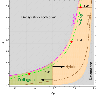
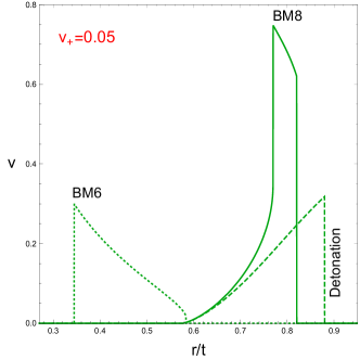
  Figure 1: Left panel: constraint on the plane $(v_{w},\alpha)$ from hydrodynamic considerations. Right panel: representative velocity profiles for plasma surrounding the bubble wall for each of the three modes with $r$ the distance from the bubble wall center and $t$ starting from the onset of the phase transition. See text for detailed explanations.

• Currently there is large uncertaintity with the determination of the bubble wall velocity $v_{w}$, so it is usually taken as a free parameter in the calculations of EWBG, EWPT and gravitational waves. It is however not entirely free as there are constraints from admitting consistent hydrodynamic solutions of the plasma at the time of phase transition, to be discussed in the following.

• Very strong phase transitions are observed for BM5, BM7, BM8 and BM9 as their values of $\alpha$ are all larger than 1. A hydrodynamical analysis of the plasma surrounding the bubbles shows that the profiles of the plasma can be classified into three categories Espinosa:2010hh : deflagrations, detonations and supersonic deflagrations (aka hybrid) KurkiSuonio:1995pp , depending on the value of the bubble wall velocity $v_{w}$. For $v_{w}$ smaller than the speed of sound in the plasma ($c_{s}=1/\sqrt{3}$), the plasma takes the form of deflagrations with the following properties: (a) the plasma ahead of the phase front flows outward with non-zero velocity; (b) the plasma inside the bubbles are static. For $c_{s}<\xi_{J}(\alpha)<v_{w}$ where $\xi_{J}$ as a function of $\alpha$ is the velocity corresponding to the Jouguet detonation Steinhardt:1981ct , a detonation profile is obtained: (a) the plasma ahead of the wall is static; (b) the plasma inside the wall flows outward. For intermediate values of $v_{w}$ with $c_{s}<v_{w}<\xi_{J}(\alpha)$, a supersonic deflagration mode is obtained with the feature that both the plasma ahead of and behind the wall flow outward. An important implication relevant for the analysis here is that there is a minumum value of $v_{w}$ when $\alpha>1/3$ for deflagration and hybrid modes Espinosa:2010hh , where $v_{w}$ smaller than this value gives no consistent solution. For benchmarks BM11 and BM12 both with $\alpha<1/3$, $v_{w}$ can take any value, while for BM5-10, there is a limited range for $v_{w}$.

  In the left panel of Fig. 1, we show on the plane of $(v_{w},\alpha)$, the resulting ranges of $v_{w}$ for BM6, BM7 and BM8, denoted by black horizontal lines that extend between the two gray region boundaries. We note that the value of $\alpha$ for BM10 is close to that of BM6, while the values of $\alpha$ for BM5 and BM9 are similar to BM8. We do not plot these cases to prevent the plot from being overcrowded. The left gray region is forbidden by the constraint mentioned above, while the right gray region gives a $v_{w}$ too fast for EWBG to work . The allowed regions in this plot are the light green region for deflagration and the brown region for supersonic deflagration. We also show three representative fluid profiles in each of the modes in the right panel of Fig. 1.

• The usual consensus for EWBG calculations is that the bubble wall velocity needs to be sufficiently small to allow diffusion of particles ahead of the wall and to produce net baryon number through the sphaleron process, with a typical value of $v_{w}=0.05$ (see for example John:2000zq ; Cirigliano:2006dg ; Chung:2009qs ; Chao:2014dpa ; Guo:2016ixx ; White:2016nbo ). However such small velocities would weaken gravitational wave production. The story changes when the hydrodynamic properties of the plasma surrounding the bubble wall are taken into account, and the dilemma between successful baryon number generation and a strong gravitational signal may be avoided. The reason is that the plasma ahead of the wall can be stirred by the expanding wall and gain a velocity in the deflagration and hybrid modes. This has the consequence that in the wall frame the plasma would hit the wall with a velocity $v_{+}$ that is different from $v_{w}$ Espinosa:2010hh ; No:2011fi and it is $v_{+}$ rather than $v_{w}$ that should enter the calculations of EWBG. While a definitive justification of this argument would require analyzing the transport behavior of the particle species surrounding the wall in the above picture, we assume tentatively that this is true in this work(see Ref. Kozaczuk:2015owa for a similar discussion on this point in the same model). The contours for a subsonic $v_{+}$ with values of $0.3$, $0.05$ and $0.01$ are shown in the left panel of Fig. 1. We can see that $v_{+}$ decreases as $\alpha$ increases for fixed $v_{w}$, with the contour $v_{+}=0$ coinciding with the boundary of the left gray region. Assuming $v_{+}=0.05$ is used for EWBG calculations, we locate the value of $v_{w}$, which corresponds to the intersection point of this contour with the horizon line of each benchmark, represented as a red point. The $v_{w}$ found in this way is used to calculate the gravitational wave energy spectrum.

With above problems properly taken care of, we can now calculate the gravitational waves resulting from the EWPT.

3.2 Gravitational Waves

A stochastic background of gravitational waves can be generated during a first order EWPT from mainly three sources: collisions of the electroweak bubbles Kosowsky:1991ua ; Kosowsky:1992rz ; Kosowsky:1992vn ; Huber:2008hg ; Jinno:2016vai ; Jinno:2017fby , bulk motion of the plasma in the form of sound waves Hindmarsh:2013xza ; Hindmarsh:2015qta and Magnetohydrodynamic (MHD) turbulence Caprini:2009yp ; Binetruy:2012ze (see Ref. Caprini:2015zlo ; Cai:2017cbj ; Weir:2017wfa for recent reviews). The total resulting energy spectrum can be written approximately as the sum of these contributions:

$$\Omega_{\text{GW}}h^{2}\simeq\Omega_{\text{col}}h^{2}+\Omega_{\text{sw}}h^{2}+\Omega_{\text{turb}}h^{2}.$$ (15)

While earlier studies of gravitational wave production from EWPT have focused on bubble collisions, recent advances in numerical simulations show that the long lasting sound waves during and after the EWPT give the dominant contribution to the gravitational wave production Hindmarsh:2013xza ; Hindmarsh:2015qta and the contribution from bubble collision can be neglected Bodeker:2017cim . From such numerical simulations, an analytical formula has been obtained for this kind of gravitational wave energy spectrum Hindmarsh:2015qta :

$$\Omega_{\textrm{sw}}h^{2}=2.65\times 10^{-6}\left(\frac{H_{\ast}}{\beta}\right)\left(\frac{\kappa_{v}\alpha}{1+\alpha}\right)^{2}\left(\frac{100}{g_{\ast}}\right)^{1/3}$$

$$\hskip 39.83368pt\times v_{w}\left(\frac{f}{f_{\text{sw}}}\right)^{3}\left(\frac{7}{4+3(f/f_{\textrm{sw}})^{2}}\right)^{7/2}\ .$$ (16)

Here $g_{\ast}$ is the relativistic degrees of freedom in the plasma, $H_{\ast}$ is the Hubble parameter at $T_{\ast}$ when the phase transition has completed and has a value close to that evaluated at the nucleation temperature $H(T_{n})$ for not very long EPWT. We take $T_{\ast}=T_{n}(1+\kappa_{T}\alpha)^{1/4}$ where the fraction of vacuum energy goes to heating the plasma is given by $\kappa_{T}\approx 1-\kappa_{v}$ Espinosa:2010hh . Moreover, $f_{\text{sw}}$ is the present peak frequency which is the redshifted value of the peak frequency at the time of EWPT($=2\beta/(\sqrt{3}v_{w})$):

$$f_{\textrm{sw}}=1.9\times 10^{-5}\frac{1}{v_{w}}\left(\frac{\beta}{H_{\ast}}\right)\left(\frac{T_{\ast}}{100\textrm{GeV}}\right)\left(\frac{g_{\ast}}{100}\right)^{1/6}\textrm{Hz}.$$ (17)

The factor $\kappa_{v}$ is the fraction of latent heat that is transformed into the bulk motion of the fluid and can be calculated as a function of ($\alpha$, $v_{w}$) by analyzing the energy budget during the EWPT Espinosa:2010hh . We note that a more recent numerical simulation by the same group Hindmarsh:2017gnf obtained a slightly enhanced $\Omega_{\text{sw}}h^{2}$ and a slightly reduced peak frequency $f_{\text{sw}}$.

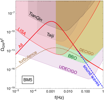
Figure 2: Gravitational wave energy spectrum for BM5 together with experimentally sensitive regions on the top. See text for more detailed explanations of this figure.

It should be noted that the above numerical simulations were performed under two important assumptions, which limit the possible applications here for some benchmarks. The first assumption is that the gravitational wave sourcing continues at the wavenumber corresponding to the thickness of the fluid shells, which is valid when the system is linear and requires the fluid velocity to be sufficiently smaller than unity. This is indeed what was adopted in the initial numerical simulations Hindmarsh:2013xza ; Hindmarsh:2015qta and in a later simulation Hindmarsh:2017gnf as well as in the recently proposed sound shell model Hindmarsh:2016lnk , aiming at understanding the origin of the shape of the gravitational wave spectra from previous simulations, which adds linearly the fluid velocity profiles when calculating the velocity power spectra. This therefore puts doubts on the effectiveness in using the above formulae for our benchmarks with large velocities. Since there is currently no available result beyond current simulations, we assume the above results hold for these cases and remind the reader of this possible issue here. The second assumption is that the sourcing of gravitational waves continues until the Hubble time. This is important since the gravitational wave energy density is directly proportional to the lifetime of the sound waves. While there is no direct numerical simulation studies confirming this, it was found to be true in Ref. Hindmarsh:2015qta ; Hindmarsh:2016lnk .

Aside from the sound waves which give the dominant gravitational wave signals, the fully ionized plasma at the time of EWPT results in MHD turbulence, giving another source of gravitational waves. When a possible helical component Kahniashvili:2008pe is neglected, the resulting gravitational wave energy spectrum can be modeled in a similar way Caprini:2009yp ; Binetruy:2012ze ,

$$\Omega_{\textrm{turb}}h^{2}=3.35\times 10^{-4}\left(\frac{H_{\ast}}{\beta}\right)\left(\frac{\kappa_{\text{turb}}\alpha}{1+\alpha}\right)^{3/2}\left(\frac{100}{g_{\ast}}\right)^{1/3}$$

$$\hskip 51.21504pt\times v_{w}\frac{(f/f_{\textrm{turb}})^{3}}{[1+(f/f_{\textrm{turb}})]^{11/3}(1+8\pi f/h_{\ast})},$$ (18)

where the peak frequency $f_{turb}$ corresponding to MHD is given by:

$$f_{\textrm{turb}}=2.7\times 10^{-5}\frac{1}{v_{w}}\left(\frac{\beta}{H_{\ast}}\right)\left(\frac{T_{\ast}}{100\textrm{GeV}}\right)\left(\frac{g_{\ast}}{100}\right)^{1/6}\textrm{Hz}.$$ (19)

Similar to $\kappa_{v}$, here the factor $\kappa_{\text{turb}}$ is the fraction of latent heat that is transferred to MHD turbulence. A recent numerical simulation shows that when $\kappa_{\rm turb}$ is parametrized as $\kappa_{\text{turb}}\approx\epsilon\kappa_{v}$, the numerical factor $\epsilon$ can vary roughly between $5\sim 10\%$ Hindmarsh:2015qta . Here we take tentatively $\epsilon=0.1$. As has been discussed in previous section, we take the value of $v_{w}$ such that they all yield $v_{+}=0.05$, a good choice for EWBG calculations.

Adding the results given in Eq. 16 and Eq. 18, we can then obtain the total gravitational wave energy density spectrum. For example, the resulting gravitational wave energy spectrum for BM5 is shown in Fig. 2. The blue dashed line denotes the gravitational wave signal from sound waves and the brown dotted line from MHD turbulence, while the total contribution is shown with the solid red line. The color-shaded regions on the top are the experimentally sensitive regions for several proposed space-based gravitational wave detectors: LISA introduced earlier, the Taiji Gong:2014mca and TianQin Luo:2015ght programs, Big Bang Observer (BBO), DECi-hertz Interferometer Gravitational wave Observatory (DECIGO) and Ultimate-DECIGO Kudoh:2005as  .

We note that astrophysical foregrounds, such as the unresolved stochastic gravitational waves from the population of white dwarf binaries in the Galaxy Klein:2015hvg , might change the above sensitivity curves slightly. While a future precise modeling of these forgrounds is definitely important in discovering the stochastic gravitational wave of cosmological origin when the detector is online and taking data, we find it is sufficient to use above sensitivity curves in this study.

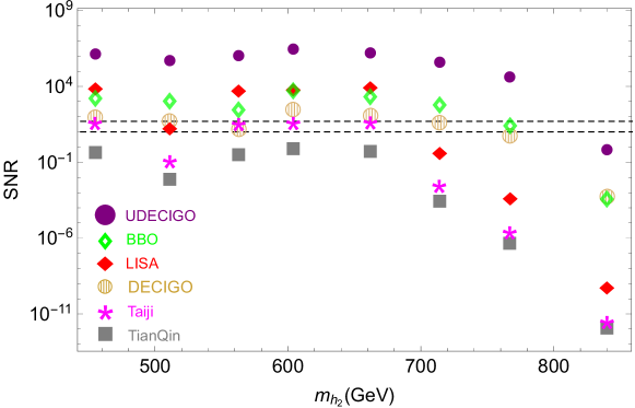
Figure 3: The SNR of the gravitational wave signals versus $m_{h_{2}}$ for the benchmarks shown in Table 1 for proposed space-based gravitational wave detectors. The two horizontal dashed lines are suggested thresholds for detection: $\text{SNR}=10$ and $\text{SNR}=50$, depending on detector configurations.

To assess the discovery prospects of the generated gravitational waves, we calculate the signal-to-noise ratio with the definition adopted by Ref. Caprini:2015zlo :

$$\text{SNR}=\sqrt{\delta\times\mathcal{T}\int_{f_{\text{min}}}^{f_{\text{max}}}df\left[\frac{h^{2}\Omega_{\text{GW}}(f)}{h^{2}\Omega_{\text{exp}}(f)}\right]^{2}},$$ (20)

where $h^{2}\Omega_{\text{exp}}(f)$ is the experimental sensitivity for the proposed experiments listed above and $\mathcal{T}$ is the mission duration in years for each experiment, assumed to be 5 here.

The additional factor $\delta$ comes from the number of independent channels for cross-correlated detectors, which equals $2$ for BBO as well as UDECIGO and $1$ for the others Thrane:2013oya .

For the LISA configurations with four links, the suggested threshold SNR for discovery is 50 Caprini:2015zlo . For the six link configurations as drawn here, the uncorrelated noise reduction technique can be used and the suggested SNR threshold is 10 Caprini:2015zlo . We show the SNR for the benchmarks versus $m_{h_{2}}$ in Fig. 3. The SNR for LISA are also added in Table. 1 for each of the benchmarks, where it shows that BM5, BM6, BM7, BM8, BM9 all have SNR larger than $10$. In particular the SNR for BM5, BM7, BM8, BM9 are all much larger than 10 and for each of these cases a very strong gravitational wave signal is expected. The last three benchmarks BM10-12 give gravitational wave signals too weak to be detected by LISA, Taiji and TianQin but some may be detected by other proposed detectors.

4 Di-Higgs Analysis

Probing double Higgs production is a major goal of the HL-LHC Koffas:2017cam ; Davey:2017obx ; Morse:2017efg ; Goncalves:2018qas ; Kim:2018uty ; Kim:2018cxf . Many theoretical studies of double Higgs production within the Standard Model have been conducted, for example in final states like $b\bar{b}\gamma\gamma$  Baur:2003gp ; Baglio:2012np ; Huang:2015tdv ; Azatov:2015oxa ; Chang:2018uwu ; Ellis:2018gqa , $b\bar{b}\tau^{+}\tau^{-}$ Baur:2003gpa ; Dolan:2012rv , $b\bar{b}W^{+}W^{-}$ Papaefstathiou:2012qe , and $b\bar{b}b\bar{b}$ deLima:2014dta ; Behr:2015oqq . Moreover, resonant di-Higgs production has also been studied by various authors CerdaAlberich:2018tkw ; Reichert:2017puo ; Huang:2017jws ; Adhikary:2017jtu ; Chen:2014ask ; Lewis:2017dme ; Chen:2017qcz in the context of EWBG Morrissey:2012db .

In this Section, we study the collider prospects of probing the benchmark points for which a large SNR for proposed gravitational wave detectors has been calculated in the previous Section. The xSM model predicts a resonant di-Higgs production $pp\rightarrow h_{2}\rightarrow h_{1}h_{1}\rightarrow b\bar{b}\gamma\gamma$ which is the channel that we will explore. Double Higgs production occurs through the three contributions depicted in Fig. 4. The non-resonant component involves the box diagram and the diagram with the trilinear Higgs coupling, while the resonant contribution corresponds to the diagram with $h_{2}$ in the $s$-channel.

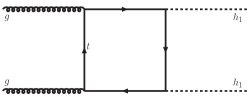
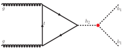
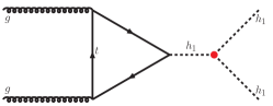
Figure 4: Representative Feynman diagrams for Di-Higgs production.

The non-resonant production cross section is strongly dependent on the size of $\lambda$, with a minimum at $\sim 0.31$ due to destructive interference between the box and the triangle diagrams. The benchmark points considered in this work all exhibit values of $\lambda$ between the SM value of $0.13$ and $0.2$, and for these points the non-resonant production cross section is suppressed compared to the SM. This suppression is partly compensated by the resonant contribution. We checked that the interference between the resonant and non-resonant contributions is negligible, so the contributions can be added incoherently.

While the resonant di-Higgs production cross section drops rapidly as the mass of $h_{2}$ is increased, the resonance peak of the $h_{1}h_{1}$ invariant mass becomes easier to identify in the tail of the background distribution as shown in Fig. 5. Taking this tradeoff into account, and noticing that BM5 and BM7 provide acceptable SNR in the gravitational waves calculation, we take these two benchmarks as the most promising ones to be probed at the HL-LHC.

We study the $b\bar{b}\gamma\gamma$ channel, which is currently the most promising channel to study the double Higgs production in the SM Baur:2003gp ; Baglio:2012np ; Huang:2015tdv ; Azatov:2015oxa ; Kim:2018uty ; Barger:2013jfa ; Dawson:2013bba ; Alves:2017ued . Recently, the fully leptonic $b\bar{b}W^{+}W^{-}$ channel was studied in the context of the xSM Huang:2017jws . This channel presents better prospects than $b\bar{b}\tau^{+}\tau^{-}$ and $b\bar{b}\gamma\gamma$ for scalar masses greater than around 450 GeV. However, the signal-to-background ratio for the BM5 and BM7 points is $\sim 0.1$ which may be an issue if the systematic uncertainties in $t\bar{t}$ backgrounds are not very well controlled. Moreover, the presence of two neutrinos precludes the reconstruction of the scalar resonance. The $b\bar{b}\gamma\gamma$ channel, on the other hand, is cleaner and permits the reconstruction of the Higgses, while its cross section is much smaller than the $b\bar{b}W^{+}W^{-}$ and $b\bar{b}\tau^{+}\tau^{-}$ channels.

In Ref. Alves:2017ued , we found that the challenge of controlling the systematic uncertainties can be addressed by judiciously adjusting the selection criteria in order to raise the signal-to-background ratio. A full comparative study across different channels using our methods would be interesting, and is left for future study.

Inclusive di-Higgs production was simulated with MadGraph5_aMC Alwall:2014hca at $\sqrt{s}=14$ TeV and NN23LO1 PDFs Ball:2013hta . We multiply the non-resonant LO rates by the NNLO QCD K-factor of 2.27 deFlorian:2013uza , the resonant one by the NNLL QCD K-factor of 2.5 Catani:2003zt and add them together to get the total cross section. This is justifiable once the contributions do not interfere. Besides the fact that the K-factors for the two contributions are similar, the kinematic cuts enhance the resonant contribution to eliminate backgrounds more efficiently. The total di-Higgs production cross section is thus approximated as described, and our signal events are weighted accordingly.

The signal cross sections are displayed in Table 2. The Higgs bosons are decayed into bottom quarks and photons with the MadSpin module of MadGraph5. We pass our simulated events to Pythia8 Sjostrand:2014zea for hadronization and showering of jets. FastJet Cacciari:2011ma is employed for clustering of jets and Delphes deFavereau:2013fsa for detector effects.

The backgrounds were also simulated within the same framework  and their total yield is shown in Table 2. The backgrounds accounted for include $b\bar{b}\gamma\gamma$, $Zh$ ($Z\to b\bar{b}$ and $h\to\gamma\gamma$), $b\bar{b}h$ ($h\to\gamma\gamma$), $t\bar{t}h\rightarrow b\bar{b}+\gamma\gamma+X$, $jj\gamma\gamma$ (the light-jets $jj$ are mistaken for $b$-jets), $b\bar{b}jj$ (the light-jets $jj$ are mistaken for photons), $c\bar{c}\gamma\gamma$ (a $c$-jet is mistagged as a $b$-jet), $b\bar{b}\gamma j$ (the light-jet is mistaken for a photon), and $c\bar{c}\gamma j$ (the $c$-jets are mistagged as $b$-jets and the light-jet as a photon), nine in total.

The first four backgrounds are generated with one extra parton radiation to better simulate the kinematic distributions, and MLM scheme Mangano:2006rw of jet-parton matching is used to avoid double counting. Their cross section normalizations were taken from Ref. Azatov:2015oxa . All the other five backgrounds are normalized by their NLO QCD rates from Alwall:2014hca but their simulation do not involve extra jets. The probability of a light-jet to be mistagged as a photon is taken to be $1.2\times 10^{-4}$, although this may be an underestimate if pileup is taken into account.

We note that several previous studies underestimated the background, and/or did not take into account light flavor jets or $c-$jets being misidentified as $b$-jets, or jets being misidentified as photons. We correctly take into account $b\bar{b}\gamma j$, $c\bar{c}\gamma\gamma$ and $c\bar{c}\gamma j$ backgrounds in our work. We assume a 70% $b$-tagging efficiency for jet $p_{T}>100$ GeV, a photon efficiency of 90% and a 20(5)% mistagging factor for $c$($j$)-jets. We refer to Alves:2017ued for further details of the background simulation and normalization.

The basic event selection requirements are two b-tagged jets with $p_{T}(b)>30$ GeV, and two photons with $p_{T}(\gamma)>20$ GeV, all within $|\eta|<2.5$. Bottom jets and photons pairs are further required to reconstruct a 125 GeV Higgs boson with $|M_{bb(\gamma\gamma)}-125|<25$ GeV, and all identified particles are isolated from any other reconstructed object within a cone of $\Delta R=0.4$ around the particle’s 3-momentum.

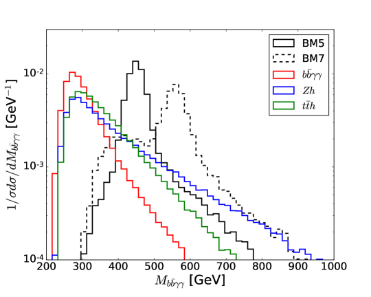
Figure 5: The $b\bar{b}\gamma\gamma$ invariant mass distribution for signals, BM5 (solid black) and BM7 (dashed black) benchmark points, and the main backgrounds.

In order to improve the statistical significance of the signal hypothesis against the background hypothesis, we used machine learning tools. First, we used an algorithm to learn the best kinematic cut thresholds in order to maximize the significance metric. This algorithm was shown to increase the significance of the non-resonant di-Higgs study in the $b\bar{b}\gamma\gamma$ channel up to 50% without relying on any other multivariate analysis Alves:2017ued . It is based on a Gaussian process algorithm built upon the backend program Hyperopt hyperopt . We refer to Alves:2017ued for a detailed description of the algorithm and its usefulness in increasing the signal significance. Many other multivariate tools can be used to improve the classification of collision events as, for example, those employed in Refs. Aaltonen:2010jr ; Baldi:2014kfa ; Alves:2016htj ; Alves:2015dya .

The kinematic variables chosen are: (1) the transverse momentum of the two leading bottom jets and the two leading photons, (2) the $\gamma\gamma$ invariant mass, (3) $\Delta R(\gamma,\gamma)$, the distance between the two leading photons, and (4) the $b\bar{b}\gamma\gamma$ invariant mass, totaling seven kinematic variables. The peak in the $b\bar{b}\gamma\gamma$ mass is helpful in isolating the signal events, and, in contrast to the standard analysis of non-resonant SM double Higgs production in this channel, makes the search efficient without many more variables. One interesting kinematic feature helps to explain the larger efficiency of the BM5 point. The heavy Higgs mass is right on the bulk of the non-resonant $h_{1}h_{1}\rightarrow b\bar{b}\gamma\gamma$ invariant mass after the basic selections, around 450 GeV, but for the BM7 point, it is displaced to 563 GeV as we can see in Fig. 5. Requiring a cut around the mass peak thus retains more non-resonant di-Higgs events for the BM5 point, raising its cut efficiency compared to BM7.

	BM5	BM7	Total Backgrounds
$\sigma$(fb)	0.012	$5.8\times 10^{-3}$	0.83
$\varepsilon_{eff}$	0.4	0.27	$5.4(1.5)\times 10^{-3}$
$\sigma\cdot\varepsilon_{eff}\cdot L$	14.4	4.7	13.5(3.7)

Table 2: The signal benchmarks, BM5 and BM7 are displayed at the first two columns and the total background is displayed in the last column. In the first row, we show the cross sections, in fb, after the basic selection discussed in the text.The second and third rows show the cut efficiencies and the number of events after optimization assuming 3 ab^-1. The numbers in parenthesis in the last column represents the backgrounds for the cuts that maximize the BM7 point.

The cuts that maximize the signal significance for BM5 and BM7 benchmark points, assuming 3 ab^-1 of integrated luminosity and 10% systematic error in the total background rates, are the following

BM5 : $$p_{T}(b)>47(30)\;\hbox{GeV},\;p_{T}(\gamma)>86(49)\;\hbox{GeV},$$ (22)

$$\Delta R_{\gamma\gamma}<4.4,\;|M_{\gamma\gamma}-125|<5\;\hbox{GeV},$$

$$|M_{b\bar{b}\gamma\gamma}-455|<38\;\hbox{GeV}$$

BM7 : $$p_{T}(b)>54(30)\;\hbox{GeV},\;\;p_{T}(\gamma)>104(40),\;\hbox{GeV},$$

$$\Delta R_{\gamma\gamma}<3.3,\;|M_{\gamma\gamma}-125|<5\;\hbox{GeV},$$

$$|M_{b\bar{b}\gamma\gamma}-563|<46\;\hbox{GeV.}$$

The cut selections for other systematics are similar. Because BM7 has a smaller production rate, the cuts learned by the algorithm were harder than the BM5 case in order to raise the significance. The cut efficiencies for the signals are almost three orders of magnitude larger than the backgrounds, as we can see in Table 2, reaching a signal to background ratio slightly larger than 1 for both signal points.

The signal significance, assuming a 10% systematic error in the total background rate is $3.2\sigma$ for the BM5, and $1.8\sigma$ for BM7, respectively, as shown in the third column of Table 3 where results for 5% and 15% systematics are also shown. Note that $S/B$, displayed in the fourth column of Table 3, increases to soften the degradation of significance with the systematics in BM5 and is kept constant for BM7. This is the job of the cut optimization program cutoptimize . A public code of the algorithm used in this work to learn the cuts and run our multivariate analysis in an automatized way will be released in the future cutoptimize .

Further improvement of the study was achieved by training boosted decision trees with
XGBoost xgb using the full representation of the events which comprise 28 kinematic variables: the transverse momentum of the two leading bottom jets $p_{T}(bb)$ and two leading photons $p_{T}(\gamma\gamma)$, the $\Delta R$ distance, the invariant masses and the Barr variable Barr:2005dz ; Alves:2007xt of all combinations of two particles, the $b\bar{b}\gamma\gamma$ mass, the azimuthal angle between the leptons and the bottoms pairs $\Delta\phi(bb,\ell\ell)$, and the missing transverse energy of the event. In order to tag $t\bar{t}h$ events we also used the number of leptons of the event. We averaged the results of a 10-fold cross validation to assess the robustness of our BDT training procedures. In order to obtain the best result possible, we tuned the BDT hyperparameters and the cut thresholds jointly. By doing this, we find the best compromise between cut-and-count and the multivariate analysis.

The BDT classification increases the signal significance for both benchmark scenarios, predicting discovery for the BM5 and evidence for BM7 for systematics ranging from 5 to 15%. In the case of BM5, a $5\sigma$ discovery might be possible for around 2 ab^-1 in the $b\bar{b}\gamma\gamma$ channel.

In the last column of Table 3 we display two significances: one by cutting on the BDT scores distributions of signal and background after tuning only the kinematic cuts but keeping BDT hyperparameters fixed, reaching $6.3\sigma$ and $3.3\sigma$ for BM5 and BM7, respectively, in the 5% systematics scenario. The other number, in parenthesis, represents the significance achieved by jointly optimizing cuts and BDT hyperparameters. In this case, the significances increase slightly for all systematics but the joint optimization algorithm learns to soften $S/B$ even further, making the significance prospects insensitive to systematic uncertainties in the background rates. The final cut on the BDT scores shown in Fig. 6 is also optimized in order to get the maximum significance possible. The typical best BDT score cut is around 0.7 which corresponds approximately to a 80% efficiency for signals and 80% rejection for backgrounds resulting in around 12(4) signal events against 3(1) expected background events for the BM5(BM7) point assuming 3 ab^-1. We use the profile likelihood formula of Ref. LiMa which approximates well the true Poissonian statistics and embodies systematic uncertainties in the background rates to compute our signal significances.

BM point	$\varepsilon_{sys}$(%)	optimized cuts($\sigma$)	S/B	BDT($\sigma$)
	5	3.4	0.9	6.3(6.4)
BM5	10	3.2	1.2	6.1(6.4)
	15	2.9	1.4	5.9(6.4)
	5	1.9	0.8	3.3(3.4)
BM7	10	1.8	0.8	3.2(3.4)
	15	1.7	0.8	3.1(3.4)

Table 3: The signal significance and the signal-to-background ratio of BM5 and BM7 benchmark points for three systematic uncertainties in the background total rates scenarios – 5, 10 and 15%. The results of the optimized cut-and-count and the corresponding $S/B$ achieved are displayed in the third and fourth columns, and the BDT analysis in the last column. Also, in the last column, we show in parenthesis the results for the joint BDT+cuts optimization.

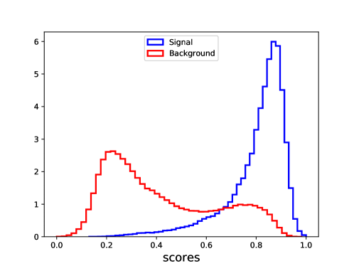
Figure 6: The normalized BDT output scores distribution for signal(BM5) and background events after joint cuts and hyperparameters optimization. A final selection is obtained by an additional cut on these distributions.

5 Conclusions

Understanding the EWPT is an important goal of current and future experiments. We have explored the complementarity of the HL-LHC and proposed space-based gravitational wave detectors in achieving this goal.

We have taken the simplest template where this complementarity can be probed - the xSM model - and studied several benchmarks that are compatible with a first order EWPT. We first calculated their gravitational wave energy spectra and signal-to-noise ratio for proposed experiments, being careful about subtle issues pertaining to the bubble wall velocity and the hydrodynamics of the plasma. Then, we took the most optimistic benchmarks and performed a collider study of double Higgs production using machine learning tools for two learning tasks: (1) to search for optimum cut thresholds and BDT hyperparameters, and (2) discriminate signal and background events with BDTs. Our results show that state-of-the-art machine learning tools can be quite powerful in probing these processes, even assuming substantial systematic uncertainties.

There are several future directions. The tension between requiring bubble wall velocities small enough to produce a net baryon number through the sphaleron process, and large enough to obtain appreciable gravitational wave production, merits further study and a more comprehensive understanding of the parameter space in concrete models. A deeper understanding of the mechanism of gravitational wave production will be needed to obtain more realistic benchmark models. On the collider side, other final states of di-Higgs, such as $b\bar{b}W^{+}W^{-}$, can be studied at these realistic benchmarks using the multivariate tools we have discussed.

6 Acknowledgments

A. Alves thanks Conselho Nacional de Desenvolvimento Científico (CNPq) for its financial support, grant 307265/2017-0. K. Sinha is supported by the U. S. Department of Energy grant de-sc0009956. T. Ghosh is supported by U. S. Department of Energy grant de-sc0010504 and in part by U. S. National Science Foundation grant PHY-125057. H. Guo would like to thank Hao-Lin Li for helpful discussions.

References

- (1) S. Profumo, M. J. Ramsey-Musolf, and G. Shaughnessy, “Singlet Higgs phenomenology and the electroweak phase transition,” JHEP 08 (2007) 010, arXiv:0705.2425 [hep-ph].
- (2) S. Profumo, M. J. Ramsey-Musolf, C. L. Wainwright, and P. Winslow, “Singlet-catalyzed electroweak phase transitions and precision Higgs boson studies,” Phys. Rev. D91 no. 3, (2015) 035018, arXiv:1407.5342 [hep-ph].
- (3) T. Huang, J. M. No, L. Pernié, M. Ramsey-Musolf, A. Safonov, M. Spannowsky, and P. Winslow, “Resonant di-Higgs boson production in the channel: Probing the electroweak phase transition at the LHC,” Phys. Rev. D96 no. 3, (2017) 035007, arXiv:1701.04442 [hep-ph].
- (4) D. E. Morrissey and M. J. Ramsey-Musolf, “Electroweak baryogenesis,” New J. Phys. 14 (2012) 125003, arXiv:1206.2942 [hep-ph].
- (5) J. R. Espinosa, T. Konstandin, J. M. No, and G. Servant, “Energy Budget of Cosmological First-order Phase Transitions,” JCAP 1006 (2010) 028, arXiv:1004.4187 [hep-ph].
- (6) J. M. No, “Large Gravitational Wave Background Signals in Electroweak Baryogenesis Scenarios,” Phys. Rev. D84 (2011) 124025, arXiv:1103.2159 [hep-ph].
- (7) A. Alves, T. Ghosh, and K. Sinha, “Can We Discover Double Higgs Production at the LHC?,” Phys. Rev. D96 no. 3, (2017) 035022, arXiv:1704.07395 [hep-ph].
- (8) J. Bergstra, “Hyperopt: Distributed asynchronous hyper-parameter optimization.” https://github.com/jaberg/hyperopt.
- (9) T. Chen and C. Guestrin, “XGBoost: A Scalable Tree Boosting System.” https://github.com/dmlc/xgboost.
- (10) Virgo, LIGO Scientific Collaboration, B. P. Abbott et al., “Observation of Gravitational Waves from a Binary Black Hole Merger,” Phys. Rev. Lett. 116 no. 6, (2016) 061102, arXiv:1602.03837 [gr-qc].
- (11) H. Audley et al., “Laser Interferometer Space Antenna,” arXiv:1702.00786 [astro-ph.IM].
- (12) C. Caprini et al., “Science with the space-based interferometer eLISA. II: Gravitational waves from cosmological phase transitions,” JCAP 1604 no. 04, (2016) 001, arXiv:1512.06239 [astro-ph.CO].
- (13) R.-G. Cai, Z. Cao, Z.-K. Guo, S.-J. Wang, and T. Yang, “The Gravitational-Wave Physics,” arXiv:1703.00187 [gr-qc].
- (14) D. J. Weir, “Gravitational waves from a first order electroweak phase transition: a review,” 2017. arXiv:1705.01783 [hep-ph]. http://inspirehep.net/record/1598112/files/arXiv:1705.01783.pdf.
- (15) P. Huang, A. J. Long, and L.-T. Wang, “Probing the Electroweak Phase Transition with Higgs Factories and Gravitational Waves,” Phys. Rev. D94 no. 7, (2016) 075008, arXiv:1608.06619 [hep-ph].
- (16) K. Hashino, M. Kakizaki, S. Kanemura, and T. Matsui, “Synergy between measurements of gravitational waves and the triple-Higgs coupling in probing the first-order electroweak phase transition,” Phys. Rev. D94 no. 1, (2016) 015005, arXiv:1604.02069 [hep-ph].
- (17) K. Hashino, M. Kakizaki, S. Kanemura, P. Ko, and T. Matsui, “Gravitational waves and Higgs boson couplings for exploring first order phase transition in the model with a singlet scalar field,” Phys. Lett. B766 (2017) 49–54, arXiv:1609.00297 [hep-ph].
- (18) A. Beniwal, M. Lewicki, J. D. Wells, M. White, and A. G. Williams, “Gravitational wave, collider and dark matter signals from a scalar singlet electroweak baryogenesis,” arXiv:1702.06124 [hep-ph].
- (19) D. Croon, V. Sanz, and G. White, “Model Discrimination in Gravitational Wave spectra from Dark Phase Transitions,” arXiv:1806.02332 [hep-ph].
- (20) S. R. Coleman and E. J. Weinberg, “Radiative Corrections as the Origin of Spontaneous Symmetry Breaking,” Phys. Rev. D7 (1973) 1888–1910.
- (21) M. Quiros, “Finite temperature field theory and phase transitions,” in Proceedings, Summer School in High-energy physics and cosmology: Trieste, Italy, June 29-July 17, 1998, pp. 187–259. 1999. arXiv:hep-ph/9901312 [hep-ph].
- (22) R. R. Parwani, “Resummation in a hot scalar field theory,” Phys. Rev. D45 (1992) 4695, arXiv:hep-ph/9204216 [hep-ph]. [Erratum: Phys. Rev.D48,5965(1993)].
- (23) D. J. Gross, R. D. Pisarski, and L. G. Yaffe, “QCD and Instantons at Finite Temperature,” Rev. Mod. Phys. 53 (1981) 43.
- (24) N. K. Nielsen, “On the Gauge Dependence of Spontaneous Symmetry Breaking in Gauge Theories,” Nucl. Phys. B101 (1975) 173–188.
- (25) H. H. Patel and M. J. Ramsey-Musolf, “Baryon Washout, Electroweak Phase Transition, and Perturbation Theory,” JHEP 07 (2011) 029, arXiv:1101.4665 [hep-ph].
- (26) W. Chao, H.-K. Guo, and J. Shu, “Gravitational Wave Signals of Electroweak Phase Transition Triggered by Dark Matter,” JCAP 1709 no. 09, (2017) 009, arXiv:1702.02698 [hep-ph].
- (27) L. Bian, H.-K. Guo, and J. Shu, “Gravitational Waves, baryon asymmetry of the universe and electric dipole moment in the CP-violating NMSSM,” arXiv:1704.02488 [hep-ph].
- (28) W. Chao, W.-F. Cui, H.-K. Guo, and J. Shu, “Gravitational Wave Imprint of New Symmetry Breaking,” arXiv:1707.09759 [hep-ph].
- (29) C. L. Wainwright, “CosmoTransitions: Computing Cosmological Phase Transition Temperatures and Bubble Profiles with Multiple Fields,” Comput. Phys. Commun. 183 (2012) 2006–2013, arXiv:1109.4189 [hep-ph].
- (30) J. M. Cline, “Baryogenesis,” in Les Houches Summer School - Session 86: Particle Physics and Cosmology: The Fabric of Spacetime Les Houches, France, July 31-August 25, 2006. 2006. arXiv:hep-ph/0609145 [hep-ph].
- (31) H. Kurki-Suonio and M. Laine, “Supersonic deflagrations in cosmological phase transitions,” Phys. Rev. D51 (1995) 5431–5437, arXiv:hep-ph/9501216 [hep-ph].
- (32) P. J. Steinhardt, “Relativistic Detonation Waves and Bubble Growth in False Vacuum Decay,” Phys. Rev. D25 (1982) 2074.
- (33) T. Konstandin and J. M. No, “Hydrodynamic obstruction to bubble expansion,” JCAP 1102 (2011) 008, arXiv:1011.3735 [hep-ph].
- (34) P. John and M. G. Schmidt, “Do stops slow down electroweak bubble walls?,” Nucl. Phys. B598 (2001) 291–305, arXiv:hep-ph/0002050 [hep-ph]. [Erratum: Nucl. Phys.B648,449(2003)].
- (35) V. Cirigliano, S. Profumo, and M. J. Ramsey-Musolf, “Baryogenesis, Electric Dipole Moments and Dark Matter in the MSSM,” JHEP 07 (2006) 002, arXiv:hep-ph/0603246 [hep-ph].
- (36) D. J. H. Chung, B. Garbrecht, M. Ramsey-Musolf, and S. Tulin, “Supergauge interactions and electroweak baryogenesis,” JHEP 12 (2009) 067, arXiv:0908.2187 [hep-ph].
- (37) W. Chao and M. J. Ramsey-Musolf, “Electroweak Baryogenesis, Electric Dipole Moments, and Higgs Diphoton Decays,” JHEP 10 (2014) 180, arXiv:1406.0517 [hep-ph].
- (38) H.-K. Guo, Y.-Y. Li, T. Liu, M. Ramsey-Musolf, and J. Shu, “Lepton-Flavored Electroweak Baryogenesis,” Phys. Rev. D96 no. 11, (2017) 115034, arXiv:1609.09849 [hep-ph].
- (39) G. A. White, A Pedagogical Introduction to Electroweak Baryogenesis. IOP Concise Physics. Morgan & Claypool, 2016.
- (40) J. Kozaczuk, “Bubble Expansion and the Viability of Singlet-Driven Electroweak Baryogenesis,” JHEP 10 (2015) 135, arXiv:1506.04741 [hep-ph].
- (41) A. Kosowsky, M. S. Turner, and R. Watkins, “Gravitational radiation from colliding vacuum bubbles,” Phys. Rev. D45 (1992) 4514–4535.
- (42) A. Kosowsky, M. S. Turner, and R. Watkins, “Gravitational waves from first order cosmological phase transitions,” Phys. Rev. Lett. 69 (1992) 2026–2029.
- (43) A. Kosowsky and M. S. Turner, “Gravitational radiation from colliding vacuum bubbles: envelope approximation to many bubble collisions,” Phys. Rev. D47 (1993) 4372–4391, arXiv:astro-ph/9211004 [astro-ph].
- (44) S. J. Huber and T. Konstandin, “Gravitational Wave Production by Collisions: More Bubbles,” JCAP 0809 (2008) 022, arXiv:0806.1828 [hep-ph].
- (45) R. Jinno and M. Takimoto, “Gravitational waves from bubble collisions: An analytic derivation,” Phys. Rev. D95 no. 2, (2017) 024009, arXiv:1605.01403 [astro-ph.CO].
- (46) R. Jinno and M. Takimoto, “Gravitational waves from bubble dynamics: Beyond the Envelope,” arXiv:1707.03111 [hep-ph].
- (47) M. Hindmarsh, S. J. Huber, K. Rummukainen, and D. J. Weir, “Gravitational waves from the sound of a first order phase transition,” Phys. Rev. Lett. 112 (2014) 041301, arXiv:1304.2433 [hep-ph].
- (48) M. Hindmarsh, S. J. Huber, K. Rummukainen, and D. J. Weir, “Numerical simulations of acoustically generated gravitational waves at a first order phase transition,” Phys. Rev. D92 no. 12, (2015) 123009, arXiv:1504.03291 [astro-ph.CO].
- (49) C. Caprini, R. Durrer, and G. Servant, “The stochastic gravitational wave background from turbulence and magnetic fields generated by a first-order phase transition,” JCAP 0912 (2009) 024, arXiv:0909.0622 [astro-ph.CO].
- (50) P. Binetruy, A. Bohe, C. Caprini, and J.-F. Dufaux, “Cosmological Backgrounds of Gravitational Waves and eLISA/NGO: Phase Transitions, Cosmic Strings and Other Sources,” JCAP 1206 (2012) 027, arXiv:1201.0983 [gr-qc].
- (51) D. Bodeker and G. D. Moore, “Electroweak Bubble Wall Speed Limit,” JCAP 1705 no. 05, (2017) 025, arXiv:1703.08215 [hep-ph].
- (52) M. Hindmarsh, S. J. Huber, K. Rummukainen, and D. J. Weir, “Shape of the acoustic gravitational wave power spectrum from a first order phase transition,” arXiv:1704.05871 [astro-ph.CO].
- (53) M. Hindmarsh, “Sound shell model for acoustic gravitational wave production at a first-order phase transition in the early Universe,” Phys. Rev. Lett. 120 no. 7, (2018) 071301, arXiv:1608.04735 [astro-ph.CO].
- (54) T. Kahniashvili, L. Campanelli, G. Gogoberidze, Y. Maravin, and B. Ratra, “Gravitational Radiation from Primordial Helical Inverse Cascade MHD Turbulence,” Phys. Rev. D78 (2008) 123006, arXiv:0809.1899 [astro-ph]. [Erratum: Phys. Rev.D79,109901(2009)].
- (55) X. Gong et al., “Descope of the ALIA mission,” J. Phys. Conf. Ser. 610 no. 1, (2015) 012011, arXiv:1410.7296 [gr-qc].
- (56) TianQin Collaboration, J. Luo et al., “TianQin: a space-borne gravitational wave detector,” Class. Quant. Grav. 33 no. 3, (2016) 035010, arXiv:1512.02076 [astro-ph.IM].
- (57) H. Kudoh, A. Taruya, T. Hiramatsu, and Y. Himemoto, “Detecting a gravitational-wave background with next-generation space interferometers,” Phys. Rev. D73 (2006) 064006, arXiv:gr-qc/0511145 [gr-qc].
- (58) A. Klein et al., “Science with the space-based interferometer eLISA: Supermassive black hole binaries,” Phys. Rev. D93 no. 2, (2016) 024003, arXiv:1511.05581 [gr-qc].
- (59) E. Thrane and J. D. Romano, “Sensitivity curves for searches for gravitational-wave backgrounds,” Phys. Rev. D88 no. 12, (2013) 124032, arXiv:1310.5300 [astro-ph.IM].
- (60) ATLAS Collaboration, T. Koffas, “ATLAS Higgs physics prospects at the high luminosity LHC,” PoS ICHEP2016 (2017) 426.
- (61) ATLAS Collaboration, W. Davey, “Search for di-Higgs production with the ATLAS detector,” PoS EPS-HEP2017 (2017) 272.
- (62) CMS Collaboration, D. M. Morse, “Latest results on di-Higgs boson production with CMS,” 2017. arXiv:1708.08249 [hep-ex]. http://inspirehep.net/record/1620209/files/arXiv:1708.08249.pdf.
- (63) D. Gonçalves, T. Han, F. Kling, T. Plehn, and M. Takeuchi, “Higgs boson pair production at future hadron colliders: From kinematics to dynamics,” Phys. Rev. D97 no. 11, (2018) 113004, arXiv:1802.04319 [hep-ph].
- (64) J. H. Kim, Y. Sakaki, and M. Son, “Combined analysis of double Higgs production via gluon fusion at the HL-LHC in the effective field theory approach,” Phys. Rev. D98 no. 1, (2018) 015016, arXiv:1801.06093 [hep-ph].
- (65) J. H. Kim, K. Kong, K. T. Matchev, and M. Park, “Measuring the Triple Higgs Self-Interaction at the Large Hadron Collider,” arXiv:1807.11498 [hep-ph].
- (66) U. Baur, T. Plehn, and D. L. Rainwater, “Probing the Higgs selfcoupling at hadron colliders using rare decays,” Phys. Rev. D69 (2004) 053004, arXiv:hep-ph/0310056 [hep-ph].
- (67) J. Baglio, A. Djouadi, R. Gröber, M. M. Mühlleitner, J. Quevillon, and M. Spira, “The measurement of the Higgs self-coupling at the LHC: theoretical status,” JHEP 04 (2013) 151, arXiv:1212.5581 [hep-ph].
- (68) P. Huang, A. Joglekar, B. Li, and C. E. M. Wagner, “Probing the Electroweak Phase Transition at the LHC,” Phys. Rev. D93 no. 5, (2016) 055049, arXiv:1512.00068 [hep-ph].
- (69) A. Azatov, R. Contino, G. Panico, and M. Son, “Effective field theory analysis of double Higgs boson production via gluon fusion,” Phys. Rev. D92 no. 3, (2015) 035001, arXiv:1502.00539 [hep-ph].
- (70) J. Chang, K. Cheung, J. S. Lee, C.-T. Lu, and J. Park, “Higgs-boson-pair production from gluon fusion at the HL-LHC and HL-100 TeV hadron collider,” arXiv:1804.07130 [hep-ph].
- (71) J. Ellis, C. W. Murphy, V. Sanz, and T. You, “Updated Global SMEFT Fit to Higgs, Diboson and Electroweak Data,” JHEP 06 (2018) 146, arXiv:1803.03252 [hep-ph].
- (72) U. Baur, T. Plehn, and D. L. Rainwater, “Examining the Higgs boson potential at lepton and hadron colliders: A Comparative analysis,” Phys. Rev. D68 (2003) 033001, arXiv:hep-ph/0304015 [hep-ph].
- (73) M. J. Dolan, C. Englert, and M. Spannowsky, “Higgs self-coupling measurements at the LHC,” JHEP 10 (2012) 112, arXiv:1206.5001 [hep-ph].
- (74) A. Papaefstathiou, L. L. Yang, and J. Zurita, “Higgs boson pair production at the LHC in the channel,” Phys. Rev. D87 no. 1, (2013) 011301, arXiv:1209.1489 [hep-ph].
- (75) D. E. Ferreira de Lima, A. Papaefstathiou, and M. Spannowsky, “Standard model Higgs boson pair production in the ( )( ) final state,” JHEP 08 (2014) 030, arXiv:1404.7139 [hep-ph].
- (76) J. K. Behr, D. Bortoletto, J. A. Frost, N. P. Hartland, C. Issever, and J. Rojo, “Boosting Higgs pair production in the final state with multivariate techniques,” Eur. Phys. J. C76 no. 7, (2016) 386, arXiv:1512.08928 [hep-ph].
- (77) ATLAS Collaboration, L. Cerda Alberich, “Search for resonant and enhanced non-resonant di-Higgs production in the channel with data at 13 TeV with the ATLAS detector,” PoS EPS-HEP2017 (2018) 687.
- (78) M. Reichert, A. Eichhorn, H. Gies, J. M. Pawlowski, T. Plehn, and M. M. Scherer, “Probing baryogenesis through the Higgs boson self-coupling,” Phys. Rev. D97 no. 7, (2018) 075008, arXiv:1711.00019 [hep-ph].
- (79) A. Adhikary, S. Banerjee, R. K. Barman, B. Bhattacherjee, and S. Niyogi, “Revisiting the non-resonant Higgs pair production at the HL-LHC,” JHEP 07 (2018) 116, arXiv:1712.05346 [hep-ph].
- (80) C.-Y. Chen, S. Dawson, and I. M. Lewis, “Exploring resonant di-Higgs boson production in the Higgs singlet model,” Phys. Rev. D91 no. 3, (2015) 035015, arXiv:1410.5488 [hep-ph].
- (81) I. M. Lewis and M. Sullivan, “Benchmarks for Double Higgs Production in the Singlet Extended Standard Model at the LHC,” Phys. Rev. D96 no. 3, (2017) 035037, arXiv:1701.08774 [hep-ph].
- (82) C.-Y. Chen, J. Kozaczuk, and I. M. Lewis, “Non-resonant Collider Signatures of a Singlet-Driven Electroweak Phase Transition,” JHEP 08 (2017) 096, arXiv:1704.05844 [hep-ph].
- (83) V. Barger, L. L. Everett, C. B. Jackson, and G. Shaughnessy, “Higgs-Pair Production and Measurement of the Triscalar Coupling at LHC(8,14),” Phys. Lett. B728 (2014) 433–436, arXiv:1311.2931 [hep-ph].
- (84) S. Dawson et al., “Working Group Report: Higgs Boson,” in Proceedings, 2013 Community Summer Study on the Future of U.S. Particle Physics: Snowmass on the Mississippi (CSS2013): Minneapolis, MN, USA, July 29-August 6, 2013. 2013. arXiv:1310.8361 [hep-ex]. https://inspirehep.net/record/1262795/files/arXiv:1310.8361.pdf.
- (85) J. Alwall, R. Frederix, S. Frixione, V. Hirschi, F. Maltoni, O. Mattelaer, H. S. Shao, T. Stelzer, P. Torrielli, and M. Zaro, “The automated computation of tree-level and next-to-leading order differential cross sections, and their matching to parton shower simulations,” JHEP 07 (2014) 079, arXiv:1405.0301 [hep-ph].
- (86) NNPDF Collaboration, R. D. Ball, V. Bertone, S. Carrazza, L. Del Debbio, S. Forte, A. Guffanti, N. P. Hartland, and J. Rojo, “Parton distributions with QED corrections,” Nucl. Phys. B877 (2013) 290–320, arXiv:1308.0598 [hep-ph].
- (87) D. de Florian and J. Mazzitelli, “Two-loop virtual corrections to Higgs pair production,” Phys. Lett. B724 (2013) 306–309, arXiv:1305.5206 [hep-ph].
- (88) S. Catani, D. de Florian, M. Grazzini, and P. Nason, “Soft gluon resummation for Higgs boson production at hadron colliders,” JHEP 07 (2003) 028, arXiv:hep-ph/0306211 [hep-ph].
- (89) T. Sjöstrand, S. Ask, J. R. Christiansen, R. Corke, N. Desai, P. Ilten, S. Mrenna, S. Prestel, C. O. Rasmussen, and P. Z. Skands, “An Introduction to PYTHIA 8.2,” Comput. Phys. Commun. 191 (2015) 159–177, arXiv:1410.3012 [hep-ph].
- (90) M. Cacciari, G. P. Salam, and G. Soyez, “FastJet User Manual,” Eur. Phys. J. C72 (2012) 1896, arXiv:1111.6097 [hep-ph].
- (91) DELPHES 3 Collaboration, J. de Favereau, C. Delaere, P. Demin, A. Giammanco, V. Lemaître, A. Mertens, and M. Selvaggi, “DELPHES 3, A modular framework for fast simulation of a generic collider experiment,” JHEP 02 (2014) 057, arXiv:1307.6346 [hep-ex].
- (92) M. L. Mangano, M. Moretti, F. Piccinini, and M. Treccani, “Matching matrix elements and shower evolution for top-quark production in hadronic collisions,” JHEP 01 (2007) 013, arXiv:hep-ph/0611129 [hep-ph].
- (93) CDF Collaboration, T. Aaltonen et al., “Observation of Single Top Quark Production and Measurement of |Vtb| with CDF,” Phys. Rev. D82 (2010) 112005, arXiv:1004.1181 [hep-ex].
- (94) P. Baldi, P. Sadowski, and D. Whiteson, “Searching for Exotic Particles in High-Energy Physics with Deep Learning,” Nature Commun. 5 (2014) 4308, arXiv:1402.4735 [hep-ph].
- (95) A. Alves, “Stacking machine learning classifiers to identify Higgs bosons at the LHC,” JINST 12 no. 05, (2017) T05005, arXiv:1612.07725 [hep-ph].
- (96) A. Alves and K. Sinha, “Searches for Dark Matter at the LHC: A Multivariate Analysis in the Mono- Channel,” Phys. Rev. D92 no. 11, (2015) 115013, arXiv:1507.08294 [hep-ph].
- (97) A. Alves, T. Ghosh, and K. Sinha, “CutOptimize: A Python package fot Cut-and-Count Optimization, to be relesead.”.
- (98) A. J. Barr, “Measuring slepton spin at the LHC,” JHEP 02 (2006) 042, arXiv:hep-ph/0511115 [hep-ph].
- (99) A. Alves and O. Eboli, “Unravelling the sbottom spin at the CERN LHC,” Phys. Rev. D75 (2007) 115013, arXiv:0704.0254 [hep-ph].
- (100) T. Li and Y.-q. Ma, “Analysis methods for results in gamma-ray astronomy,” Astrophys. J. 272 (1983) 317.