Immigration-induced phase transition in a regulated multispecies birth-death process

Abstract

Power-law-distributed species counts or clone counts arise in many biological settings such as multispecies cell populations, population genetics, and ecology. This empirical observation that the number of species $c_{k}$ represented by $k$ individuals scales as negative powers of $k$ is also supported by a series of theoretical birth-death-immigration (BDI) models that consistently predict many low-population species, a few intermediate-population species, and very high-population species. However, we show how a simple global population-dependent regulation in a neutral BDI model destroys the power law distributions. Simulation of the regulated BDI model shows a high probability of observing a high-population species that dominates the total population. Further analysis reveals that the origin of this breakdown is associated with the failure of a mean-field approximation for the expected species abundance distribution. We find an accurate estimate for the expected distribution $\langle c_{k}\rangle$ by mapping the problem to a lower-dimensional Moran process, allowing us to also straightforwardly calculate the covariances $\langle c_{k}c_{\ell}\rangle$. Finally, we exploit the concepts associated with energy landscapes to explain the failure of the mean-field assumption by identifying a phase transition in the quasi-steady-state species counts triggered by a decreasing immigration rate.

I Introduction

High-dimensional stochastic models are important across many fields of science and often arise in biological contexts such as T cell receptor (TCR) diversity in immunology zarnitsyna2013estimating , species abundance and diversity in ecology mcgill2007species , and populations in cellular barcoding experiments goyal2015mechanisms . T cells in jawed vertebrates can be classified into multiple subpopulations, each corresponding to different T cell receptor (TCR) subtypes produced in the thymus. Here the number of T cells $n_{i}$ expressing the $i^{\rm th}$ receptor represents the $i^{\rm th}$ dimension. In this setting the large number of different TCRs ($1\leq i\leq\Omega$, $\Omega\sim 10^{6}-10^{8}$) present in an organism allows its adaptive immune system to recognize and respond to a wide range of antigens that it might encounter. Multispecies ecological communities are another example of high-dimensional systems. If the habitat of interest is an island, then $n_{i}$ quantifies the number of animals of species $i$ on the island. The gut is also a habitat for many coexisting species of bacteria that make up the microbiome MICROBIAL_GUT . Finally, DNA-tagging and sequencing technology has allowed in vivo tracking of multiple hematopoietic clones, each of which was derived from a unique hematopoietic stem cell that carries a unique DNA tag zarnitsyna2013estimating ; kim2014dynamics ; sun2014clonal ; biasco2016vivo ; koelle2017quantitative , resulting in clonal-tracking data of very high dimensions goyal2015mechanisms ; SONG_BLOOD .

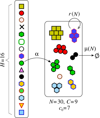
Figure 1: A simple $H$-species birth-death-immigration process in which an external fixed “source” always contains $H$ individuals, each of a different species. This source may represent uniquely tagged stem cells, a “mainland” from which species emigrate, or the thymus that outputs naive T cell clone, each expressing a different T cell receptor. Each cell in the source buds off with rate $\alpha$ a daughter cell into the system but remains intact. All individuals in the system can proliferate with rate $r(N)$ and dies with rate $\mu(N)$, where $N$ is the total population in the system. A specific configuration with $H=16$ and $N=30$ is depicted. Here, $C=9$ represents the number of different species that exist in the system. $c_{0}$ represents the number of species in the source that are not represented in the system.

The simplest single-compartment mathematical structure that is common to all the multispecies systems mentioned above is the birth-death-immigration (BDI) processes shown in Fig. 1. The source of immigration into the system is a fixed “source” population of $H$ different individuals, each of a different species. In the T cell setting, the possible number of different receptors that can be produced by the thymus is $H>10^{15}$ LAYDON while in typical barcoding experiments $H\approx 10^{3}-10^{6}$ different tags can be implanted kim2014dynamics . After immigration into the system, the individuals can proliferate with rate $r(N)$ and die with rate $\mu(N)$, both possibly function of the total population $N$. In the configuration shown in Fig. 1, the maximum number of different species is $H=16$ and the number of individuals of each species is $n_{1}=7,n_{2}=5,n_{3}=n_{4}=4,n_{5}=3,n_{6}=n_{7}=n_{8}=2,n_{9}=1$. We have labeled the species $i$ according to decreasing population. In this work, the terms “clones” and “species” are interchangeable and “clones” will only be used to refer to different tags in barcoding experiments and different T-cell receptor (TCR) types.

Such high-dimensional stochastic systems are generally difficult to study because of the “curse of dimensionality.” The evolution of the full probability distribution $P({\bf n})\equiv P(\{n_{1},n_{2},...,n_{H}\})$ is unintuitive and computationally intractable DESSALLES . It also contains more information than necessary if we consider only neutral species and their identities are not relevant. Describing the system in terms of moments such as $\langle n_{i}\rangle$ and $\langle n_{i}n_{j}\rangle$ reduces the model complexity and allows one to track the dynamics of specific species goyal2015mechanisms , but does not directly capture the species size distribution resulting from the relevant stochastic processes. Another approach is to use single-quantity metrics such as species richness, Simpson’s diversity, Shannon’s diversity, or the Gini index to describe and compare various ecological communities. Such diversity measures can be overly simplistic and can lead to different conclusions depending on the diversity index used. Thus, a description of intermediate complexity is desired.

In ecology, a commonly used measure is the species abundance distribution (SAD) that counts the number of different species encountered in a community mcgill2007species . In the language of clonal dynamics, it is the count of the number of species or “clones” that are each represented by $k$ individuals as depicted in Fig. 2 goyal2015mechanisms :

$${c}_{k}=\sum_{i=1}^{H}\mathds{1}(n_{i},k),$$ (1)

Here $\mathds{1}(x,y)$ is the identity function which takes on the value 1 when $x=y$ or 0 otherwise. The species-count ${c}_{k}$ represents a one-dimensional vector of numbers indexed by $k=0,1,...$ and gives a more comprehensive picture of how the clone/species are distributed compared to that of a single index. By construction, the species count $c_{k}$ also obeys the constraints

$$c_{0}+\sum_{k=1}^{\infty}c_{k}=H,\qquad\sum_{k=0}^{\infty}kc_{k}=N.$$ (2)

Species counts are useful in describing numbers of rare or abundant species especially when their identities are not important. Examples of such as systems include genetically barcoded, virally tagged, or TCR-decorated jin2013quantifying ; zarnitsyna2013estimating ; qi2014diversity ; goyal2015mechanisms ; desponds2016fluctuating cellular clones, microbial populations hill2003using ; hong2006predicting , and ecological species 10.2307/j.ctt7rj8w ; mcgill2007species ; guisan2005predicting .

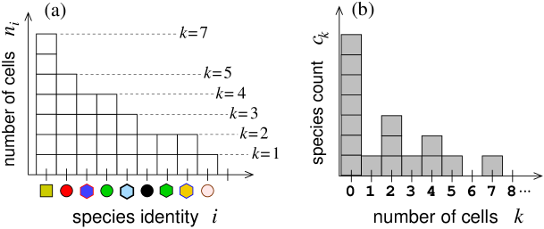
Figure 2: Definition of species counts corresponding to the configuration in Fig. 1. (a) In the cell-count representation $n_{i}$ is the number of cells of species $i$ detected in a sample. (b) ${c}_{k}$ is the number of different species that are represented by exactly $k$ cells in a sample. A given set $\{n_{i}\}$ uniquely determines the corresponding ${c}_{k}\equiv\sum_{i=1}^{\infty}\mathds{1}(n_{i},k)$. However, one cannot recover $n_{i}$ from ${c}_{k}$ since species identity information is lost when transforming from $n_{i}$ to ${c}_{k}$.

A universally observed feature in empirical studies across all these fields is a “hollow curve distribution” for $c_{k}$, where few highly populous species and many low-population species arise mcgill2007species . Theoretical studies have attempted to explain these observations by proposing various physical models, including neutral models with constant immigration, birth, and death rates motomura1932statistical ; fisher1943relation ; kendall1948some ; DESSALLES , time-dependent birth and death kendall1948generalized , cell-wise and species-wise heterogeneities desponds2016fluctuating , and intra-species carrying capacities volkov2005density .

Multi-clonal/multi-species models with fluctuating total population size commonly arise in the evolutionary biology and physics communities parsons2008absorption ; chotibut2015evolutionary ; constable2016demographic ; chotibut2017population ; constable2017mapping . Most of the attention has been on computing expected values of population counts rather than species abundance distributions. For example, Parsons et al. parsons2008absorption used a neutral and quasi-neutral birth-death model with carrying capacity and studied the mean fixation time of any species.

In ecology and immunology, the literature on the distribution $\langle c_{k}\rangle$ is rich. For example, Volkov et al. volkov2005density considered an intra-species carrying capacity that balances the birth and death rates of each species. However, they did not consider a global carrying capacity that regulates the dynamics of the population across all species. In this case, no interactions arise among the species and the mean-field results are accurate. Other theories considered competition for resources (such as T cell proliferation competing for stimuli from self-peptides lythe2016many ; desponds2016fluctuating ; eftimie2016mathematical ), but the resources were modeled as evolving variables of the system and explicit solutions could be found only in very simple cases. None of these previous studies have treated global interactions that correlate populations across all clones/species, an important ingredient in studies of interacting populations.

Stochastic simulations of a neutral BDI model that includes a simple global carrying capacity exhibit distributions of $\langle c_{k}\rangle$ that differ qualitatively from those of the above-mentioned studies. Under a high immigration rate, the classical power law distribution of $\langle c_{k}\rangle$ (with an exponential cutoff) remains an accurate representation of our simulated results. However, as the immigration rate is decreased, a single large-population species emerges. Such single-species dominance is not captured by classical mean-field theories. Through further analysis that more accurately includes the interactions between species populations, we find that a low immigration rate induces a phase transition to bistability in species populations. The mean-field approximation, which was explicitly or implicitly assumed in previous studies, breaks down near the new local stable state where the ensemble average of $c_{k}$ follows a different distribution.

In this paper, we introduce the simple idea of transforming the problem of calculating the $q^{\rm th}$ moment of $c_{k}$ to the problem of solving a $(q+1)$-dimensional process described by the population vector $\{n_{1},~{},n_{2},~{}...,~{}n_{q},~{}N^{\prime}\}$. This process can be further approximated by a $q$-dimensional Moran model that imposes a fixed total population. We use this approach to accurately calculate the $1^{\rm st}$ and $2^{\rm nd}$ moments of $c_{k}$ under general functional forms of the carrying capacity. We then exploit ideas from energy landscapes to identify the key parameters controlling a phase transition of the general multi-species BDI process that explains the failure of previously used mean-field assumptions.

II Classical formulation and mean-field assumption

Here, we develop the stochastic dynamics of the BDI process depicted in Fig. 1. In the language of clonally tracked stem cell differentiation, the probability of a stem cell carrying any specific tag asymmetrically differentiating to produce a progenitor cell within infinitesimal time $\mbox{d}t$ is $\alpha\mbox{d}t$. We will assume that there is a fixed number $H$ of stem cells or “source” individuals. The probability for any progenitor cell to divide into two new identical progenitor cells (birth) within $\mbox{d}t$ is $r\mbox{d}t$ and the probability of it dying in $\mbox{d}t$ is $\mu\mbox{d}t$.

We will further assume the particle dynamics are coupled in a species-independent way, leading to identical (but not independent) statistics of the populations of each species. The canonical implementation of such a “global” neutral interaction is through a birth rate $r(N)$ and/or death rate $\mu(N)$ which depend only on the total population $N\equiv\sum_{i=1}^{H}n_{i}=\sum_{\ell}\ell c_{\ell}$. Thus, the total population $N$ can be “decoupled” and completely described by its own master equation,

$$\begin{array}[]{l}\displaystyle{\partial P(N,t)\over\partial t}=\alpha H[P(N-1)-P(N)]\\ \>\hskip 51.21504pt+r(N-1)(N-1)P(N-1)-r(N)NP(N)\\ \>\hskip 51.21504pt+\mu(N+1)(N+1)P(N+1)-\mu(N)NP(N),\end{array}$$ (3)

from which moments of $N$ can be computed. The higher-dimensional master equation obeyed by the full multispecies distribution $P(\{n_{j}\};t)$ is explicitly given in Appendix A.

Let us denote the ensemble (not time) average of a quantity by $\langle\cdot\rangle$. Thus, $\langle n_{i}(t)\rangle\equiv\sum_{\{n_{j}\}}n_{i}P(\{n_{j}\};t)$ represents the expected population of the $i^{\rm th}$ species. By using Eqs. (3) and (37), we can show that the expected subpopulation $\langle n_{i}(t)\rangle$ and total population $\langle N(t)\rangle$ for the BDI process obeys

$$\frac{\mbox{d}\langle n_{i}\rangle}{\mbox{d}t} =\alpha+\langle(r(N)-\mu(N))n_{i}\rangle,$$

$$\frac{\mbox{d}\langle N\rangle}{\mbox{d}t} =\alpha H+\langle(r(N)-\mu(N))N\rangle.$$ (4)

In Appendix B, we also explicitly derive the equation for $\langle c_{k}(t)\rangle$,

$${\mbox{d}\langle c_{k}\rangle\over\mbox{d}t}=\alpha(\langle c_{k-1}\rangle-\langle c_{k}\rangle)+\langle r(N)\left[(k-1)c_{k-1}-kc_{k}\right]\rangle+\langle\mu(N)\left[(k+1)c_{k+1}-kc_{k}\right]\rangle,$$ (5)

from the master equation for $P(c_{0},c_{1},c_{2},\ldots;t)$. This evolution equation indicates that immigration (at rate $\alpha$) of an individual from a species with population $n_{i}=k$ increases its size by 1, thereby decreasing $c_{k}$ by 1 but increasing the number of species with population $k+1$, $c_{k+1}$, by 1. Cellular birth and death have similar effects, but their corresponding rates are proportional to the species population $k$ (the number of individuals/cells in the species). In the rest of this paper we will be interested in evaluating the steady-state values of $\langle c_{k}\rangle$.

II.1 Constant rates

In the simplest scenario of constant birth and death rates, one can write goyal2015mechanisms

$${\mbox{d}\langle c_{k}\rangle\over\mbox{d}t}=\alpha(\langle c_{k-1}\rangle-\langle c_{k}\rangle)+r[(k-1)\langle{c_{k-1}}\rangle-k\langle{c_{k}}\rangle]+\mu[(k+1)\langle c_{k+1}\rangle-k\langle c_{k}\rangle].$$ (6)

If $r<\mu$, a stable steady state can be found:

$$\langle{c_{k\geq 1}^{*}}\rangle=\frac{\alpha H}{rk!}\frac{(\frac{r}{\mu})^{k}(1-\frac{r}{\mu})^{\alpha/r}}{\frac{\alpha}{r}+k}\prod_{\ell=1}^{k}\left(\frac{\alpha}{r}+\ell\right),\quad\,\langle{c}_{0}^{*}\rangle=H-\sum_{k=1}^{\infty}\langle{c_{k}^{*}}\rangle=H\left(1-\frac{r}{\mu}\right)^{\alpha/r}.$$ (7)

In the $\alpha/r\to 0^{+}$ limit, the species counts monotonically decay as

$$\langle c_{k\geq 1}^{*}\rangle\approx H\left({\alpha\over r}\right)\left(1-{r\over\mu}\right)^{\alpha/r}\left({r\over\mu}\right)^{k}{1\over k}.$$ (8)

II.2 Carrying capacity and mean-field approximation

Now, assume that $r(N)$ decreases with $N$ and/or $\mu(N)$ increases with $N$, and that $\lim_{N\to\infty}r(N)/\mu(N)<1$. These conditions on $r(N)$ and $\mu(N)$ guarantee that $n_{i}$ and $c_{k}$ are bounded even if $r(N)>\mu(N)$ for some finite $N$. Terms of the form $\langle{r(N)c_{k}}\rangle$ in Eq. (5) cannot be approximated by factoring because $r(N)$ depends on $c_{k}$ through the stochastic variable $N\equiv\sum_{\ell}\ell c_{\ell}$ defined in Eq. (2). Nonetheless, to make headway, a mean-field method is often invoked to simplify Eq. (4) and Eq. (5). Upon fully factorizing interaction terms such as $\langle r(N)c_{k}\rangle\approx r(\langle N\rangle)\langle c_{k}\rangle$ and $\langle r(N)N\rangle\approx r(\langle N\rangle)\langle N\rangle$, we can approximate Eqs. (4) and (5) as

$$\frac{\mbox{d}\langle N\rangle}{\mbox{d}t}\approx ~{}\alpha H+\langle(r(\langle N\rangle)-\mu(\langle N\rangle))\langle N\rangle\equiv f(\langle N\rangle),$$ (9)

$${\mbox{d}\langle c_{k}\rangle\over\mbox{d}t}\approx ~{}\alpha(\langle c_{k-1}\rangle-\langle c_{k}\rangle)+r(\langle N\rangle)\left[(k-1)\langle c_{k-1}\rangle-k\langle c_{k}\rangle\right]$$

$$\quad+\mu(\langle N\rangle)\left[(k+1)\langle c_{k+1}\rangle-k\langle c_{k}\rangle\right].$$ (10)

By first solving Eq. (9) we can input $\langle N(t)\rangle$ into Eq. (10) and explicitly solve for $\langle c_{k}(t)\rangle$. The steady-state solution to $\langle N\rangle$, $\langle N^{*}\rangle$, is defined in Eq. (9) by $f(\langle N^{*}\rangle)=0$ and the requirement that $\langle N^{*}\rangle>0$ requires $[df(\langle N\rangle)/d\langle N\rangle]_{\langle N^{*}\rangle}\equiv f^{\prime}(\langle N^{*}\rangle)\equiv r^{\prime}(\langle N^{*}\rangle)-\mu^{\prime}(\langle N^{*}\rangle)<0$. The steady state values of $\langle c_{k}\rangle$ can be reached only after the steady state of $\langle N\rangle$ is reached and $r(\langle N\rangle)$ and $\mu(\langle N\rangle)$ approach constant values.

We show in Appendix C that this deterministic description breaks down after an exponentially long time when the immigration rate $\alpha$ is sufficiently small. The reason is that for $\alpha=0$, $N=0$ becomes an absorbing boundary in the full stochastic model. Thus, when $\alpha=0$, the $\langle N^{*}\rangle$ we find from $f(\langle N^{*}\rangle)=0$ is actually a quasi-steady state (QSS) even though Eq. (9) indicates a stable deterministic equilibrium $\langle N^{*}\rangle$ for physically reasonable functions $r(\langle N\rangle)$ and $\mu(\langle N\rangle)$.

Focusing on evaluating the QSS value of $\langle c_{k}\rangle$, $\langle c_{k}^{*}\rangle$, before the final extinction that occurs over exponentially long times, we denote $r(\langle N^{*}\rangle)\equiv r^{*}$ and $\mu(\langle N^{*}\rangle)\equiv\mu^{*}$ as the rates of birth and death at QSS. The QSS solution $\langle c_{k}^{*}\rangle$ can be written in the same form as Eq. (7),

$$\langle c_{k\geq 1}^{*}\rangle=\frac{\alpha H}{r^{*}k!}\frac{(\frac{r^{*}}{\mu^{*}})^{k}(1-\frac{r^{*}}{\mu^{*}})^{\alpha/r^{*}}}{\frac{\alpha}{r^{*}}+k}\prod_{\ell=1}^{k}\left(\frac{\alpha}{r^{*}}+\ell\right),\quad\langle c_{0}^{*}\rangle=H-\sum_{k=1}^{\infty}\langle c_{k}^{*}\rangle=H\left(1-\frac{r^{*}}{\mu^{*}}\right)^{\alpha/r^{*}}\!\!\!\!.$$ (11)

Here, $\langle c_{k}^{*}\rangle$ corresponds to the mean QSS species-count under the mean-field approximation which we expect to be different from the exact solution. In the $\alpha/\mu^{*},\alpha/r^{*}\to 0^{+}$ limit, the expected species count $\langle c_{k\geq 1}^{*}\rangle$, as in Eq. (8), is monotonic in $k$:

$$\langle c_{k\geq 1}^{*}\rangle\approx H\left({\alpha\over r^{*}}\right)\left(1-{r^{*}\over\mu^{*}}\right)^{\alpha/r^{*}}\left({r^{*}\over\mu^{*}}\right)^{k}{1\over k}.$$ (12)

However, under regulation, $r^{*}/\mu^{*}\approx 1-{\cal O}(\alpha/\mu^{*})$ resulting in a long-tail $k$-dependence of $\langle c_{k}^{*}\rangle$. Although the amplitude of $\langle c_{k\geq 1}^{*}\rangle$ is proportional to $\alpha/r^{*}$, it is constructed to obey the mean total population constraint $\langle N^{*}\rangle=\sum_{k=1}^{\infty}k\langle c_{k}^{*}\rangle$ which is reflected in the long-tail property of the mean-field approximation to $\langle c_{k}^{*}\rangle$.

II.3 Failure of the mean-field approximation to $\langle c_{k}^{*}\rangle$ in the slow immigration regime

To concretely investigate the errors incurred under a mean-field assumption, we first focus explicitly on a logistic growth law for the total population defined by

$$r(N)=p\left(1-\frac{N}{K}\right),\qquad\mu(N)=\mu,$$ (13)

where $p$ is the maximal birth rate and $K$ is the carrying capacity parameter. The mean-field solution for the total population is

$$\langle N^{*}\rangle =\frac{K}{2}\left(1-{\mu\over p}\right)\left[1+\sqrt{1+\frac{4\alpha Hp}{(p-\mu)^{2}K}}\right]$$

$$=K\left(1-{\mu\over p}\right)+\frac{\alpha Hp}{p-\mu}+{\cal O}(1/K).$$ (14)

In many examples, such as progenitor cells, $K\gg 1$ and $\langle N^{*}\rangle\sim K$ is large except when $\mu$ approaches or exceeds $p$.

We are now in a position to use $\langle N^{*}\rangle$ to determine $r^{*}$ and evaluate the mean-field approximation for $\langle c_{k}^{*}\rangle$ (Eq. (11)). In Fig. 3 we compare numerically evaluated mean-field solutions of $\langle c_{k}^{*}\rangle$ with Monte-Carlo simulations of the underlying BDI process for various values of $\alpha$.

For small $\alpha$, such as $10^{-8}$ used to generate Fig. 3(a), Eq. (11) fails to capture the peak arising in $\langle c_{k}^{*}\rangle$ at $k\approx\langle N^{*}\rangle$. In the singular limit $\alpha\rightarrow 0$, the mean-field solution $\langle c_{k\geq 1}^{*}\rangle\rightarrow 0$ and $\langle c_{0}^{*}\rangle\rightarrow H$ but nonetheless, by construction, satisfies $\sum_{k=1}^{\infty}k\langle c_{k}^{*}\rangle\rightarrow\langle N^{*}\rangle$. However, in the simulated $\langle{c}_{k}^{*}\rangle$, the small peak at large size $k\approx\langle N^{*}\rangle$ signals that a single species has come to dominate the total population. The number of species not in the system is thus $\langle{c}_{0}^{*}\rangle\approx H-1$. One species, typically the first to have immigrated, has taken over the system squeezing out all others that try to immigrate when the immigration rate $\alpha$ is small. This peak in $\langle c_{k}^{*}\rangle$ near $k\approx\langle N^{*}\rangle$ is completely missed by the mean-field approximation. The mean-field approximation also inaccurately captures the rapid decay in $\langle c_{k}^{*}\rangle$ for $k>\langle N^{*}\rangle$ due to exhaustion of the population in the single size-$k$ species.

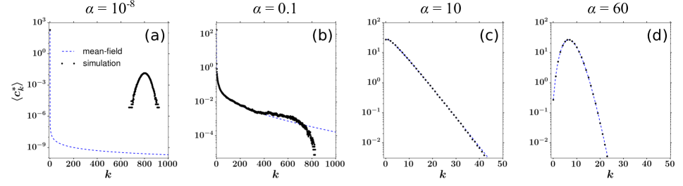
Figure 3: Comparison of steady-state species-count distributions from simulations (black dots) to those computed from the mean-field approximation (dashed blue curves) using the logistic growth model of Eq. (13) and (a) $\alpha=10^{-8}$, (b) $\alpha=0.1$, (c) $\alpha=10$, and (d) $\alpha=60$. Other parameters used are $\mu=10,~{}p=20,~{}K=1600,~{}H=200$. The resulting $N^{*}$ are $800,~{}840,~{}4800$, and $24800$, respectively. The mean-field approximation $\langle c_{k}^{*}\rangle$ breaks down for small $\alpha$ completely missing the peak at $k\approx\langle N^{*}\rangle$ in (a). Also, note the log scale and the absence of simulations that capture the rare configurations in (a) where $k\neq\langle N^{*}\rangle$.

When $\alpha$ is still relatively small as in Fig. 3(b), the simulated $\langle c_{k}^{*}\rangle$ is dominated by many low-population species, with a slow decay with size $k$ followed by a faster decay in $k$, again due to mass depletion. At this modest immigration rate, high-population species do not have the opportunity to establish and more intermediate-sized species arise at the expense of very high-population species but the simulated result $\langle c_{k}^{*}\rangle$ remains monotonic. Nevertheless, the mean-field approximation of Eq. (11) still fails to capture the fast decay of $\langle c_{k}^{*}\rangle$ for large $k$.

For even larger $\alpha$, the preferred total population increases. Since the total number of species remains capped at $H$, the mean number of individuals/cells per species increases. The distribution $P(n_{1})$ peaks at higher values of $n_{1}$ thereby forming a peak in $\langle c_{k}^{*}\rangle$ at size $k\ll\langle N^{*}\rangle$. The larger-$\alpha$ cases shown in Fig. 3(c-d) are accurately described by the mean-field approximation of $\langle c_{k}^{*}\rangle$ for all values of $k$.

III Proposed Model for $\langle{\bf c}^{q}\rangle$

The challenge in solving Eq. (5) lies in the nonseparable terms $\langle r(N)c_{k}\rangle$. Even in the simple case of logistic growth where $r(N)$ is linear, the $\langle r(N)c_{k}\rangle$ terms include second-moments $\langle c_{k}c_{\ell}\rangle$, which usually cannot be approximated by $\langle c_{k}\rangle\langle c_{\ell}\rangle$. If one attempts to solve Eq. (5) for the time-dependent or steady-state solution $\langle c_{k}^{*}\rangle$, one encounters the so-called “moment closure” problem, where the solution of the $1^{\rm st}$ moment $\langle c_{k}\rangle$ depends on $2^{\rm nd}$ moments $\langle c_{k}c_{\ell}\rangle$, which in turn depends on $3^{\rm rd}$ moments, and so on COLIN2009 . There is usually no closed-form solution or easy approximation to such problems. In the rest of this section, we develop an alternative approach.

III.1 Transformation of the problem

A complete description would be an $H$-dimensional model for the distribution $P(\{n_{1},n_{2},\ldots,n_{H}\};t)$. However, by using the definition of $c_{k}$ in Eq. (1), assuming the initial populations of all species are identical $n_{1}(0)=n_{2}(0)=\ldots=n_{H}(0)$ and indistinguishability among species, one can easily show that (Appendix D)

$$\langle{c}_{k}(t)\rangle=HP(n_{1}=k;t),$$ (15)

where $P(n_{1};t)=\sum_{n_{2}=0}^{\infty}\cdots\sum_{n_{H}=0}^{\infty}P(\{n_{1},n_{2},\ldots,n_{H}\};t)$ is the single-dimensional marginal distribution. Here, the singling out of species 1 is arbitrary. The assumption of identical initial species populations is not needed in the long time QSS limit as long as different initial distributions $c_{k}(0)$ converge to a unique $\langle c_{k}^{*}\rangle$. Thus, at QSS $\langle{c}_{k}^{*}\rangle=HP(n_{1}=k;t\to\infty)$ always holds. Intuitively, the expected fraction of all species that have size $k$ is the probability that any one species is of size $k$.

We can write the master equation for the BDI process of a single species with population $n_{1}$ as

$$\begin{array}[]{l}\displaystyle{\partial P(n_{1};t)\over\partial t}=\alpha[P(n_{1}-1)-P(n_{1})]+r(N)\left[(n_{1}-1)P(n_{1}-1)-n_{1}P(n_{1})\right]\\ \>\hskip 72.26999pt+\mu(N)\left[(n_{1}+1)P(n_{1}+1)-n_{1}P(n_{1})\right]\end{array}$$ (16)

where $N(t)$ represents one trajectory of the random process $N=n_{1}+n_{2}+\ldots+n_{H}$ which we might approximate using the deterministic solution to Eq. (4). Equation (16) has the exact same form as the right-hand side of Eq. (10) for $\langle c_{k}\rangle$. However, in the presence of other species or clones, it is immediately clear that Eq. (16) is not a complete description for $n_{1}$ since the variable $N$ depends on the population of all species. Species “independence” breaks down through the $r(N)$ and $\mu(N)$ terms. All species compete with each other for the limited sources in the environment through their shared and regulated birth and death rates.

Eq. (15) remains exact (Appendix D) since the population dynamics are neutral and all species start with the same initial size. One still needs to solve any individual species’ marginal probability distribution $P(n_{1})$ given that all species, including itself can affect it. Formally, this corresponds to first solving the full distribution $P(\{n_{1},~{}n_{2},~{}...,~{}n_{H}\})$ before summing over all other populations $\{n_{2},~{}...,~{}n_{H}\}$. Since we are not concerned about the detailed configurations of $\{n_{2},~{}...,~{}n_{H}\}$, but rather their combined effects on $n_{1}$. Therefore, we can lump species 2 through $H$ into an effective “bath” species whose size is $N^{\prime}=n_{2}+...+n_{H}$. This effective species has a birth rate $N^{\prime}r(n_{1}+N^{\prime})$, a death rate $N^{\prime}\mu(n_{1}+N^{\prime})$, and an immigration rate $(H-1)\alpha$. Eq. (16) is now coupled to the master equation

$${\partial P(N^{\prime};t)\over\partial t}= \,\alpha(H-1)[P(N^{\prime}-1)-P(N^{\prime})]+r(N)\left[(N^{\prime}-1)P(N^{\prime}-1)-N^{\prime}P(N^{\prime})\right]$$

$$\quad+\mu(N)\left[(N^{\prime}+1)P(N^{\prime}+1)-N^{\prime}P(N^{\prime})\right].$$ (17)

One usually combines Eqs. (16) and (17) together into a 2D master equation

$$\frac{\partial P(n_{1},N^{\prime};t)}{\partial t}= \,\alpha[P(n_{1}-1,N^{\prime})-P(n_{1},N^{\prime})]$$

$$+\alpha(H-1)[P(n_{1},N^{\prime}-1)-P(n_{1},N^{\prime})]$$

$$+r(N-1)\left[(n_{1}-1)P(n_{1}-1,N^{\prime})+(N^{\prime}-1)P(n_{1},N^{\prime}-1)\right]$$

$$+\mu(N+1)\left[(n_{1}+1)P(n_{1}+1,N^{\prime})+(N^{\prime}+1)P(n_{1},N^{\prime}+1)\right]$$

$$-[r(N)+\mu(N)]\left[n_{1}P(n_{1},N^{\prime})+N^{\prime}P(n_{1},N^{\prime})\right].$$ (18)

The 2D problem can be approximated by a 1D problem when $n_{1}\ll N^{\prime}$ and $r(N)\approx r(N^{\prime})$. The birth rate is approximately regulated by the “bath” population $N^{\prime}$ which leads to a decoupling from $n_{1}$. Similarly, when $n_{1}\gg N^{\prime}$, $r(N)\approx r(n_{1})$ and the birth rate is approximately independent of $N^{\prime}$. In either limit, the problem is approximately one-dimensional and can be modeled using a 1D master equation for $P(n_{1})$ [Eq. (16)] or $P(N^{\prime})$ [Eq. (3)] correspondingly. However, when $n_{1}$ and $N^{\prime}$ are comparable in size, one needs to evaluate the full 2D distribution $P(n_{1},N^{\prime})$ and marginalise over $N^{\prime}$ to obtain $P(n_{1})=\sum_{N^{\prime}=0}^{\infty}P(n_{1},N^{\prime})$ and

$$\langle c_{k}(t)\rangle=HP(n_{1}=k;t)=H\sum_{N^{\prime}=0}^{\infty}P(n_{1}=k,N^{\prime};t).$$ (19)

This approach can be extended to higher dimensions to determine higher moments of $c_{k}(t)$, which are important for characterizing the variability of species size distributions. Covariances ${\rm cov}(c_{k},c_{\ell})\equiv\langle{c}_{k}{c}_{\ell}\rangle-\langle{c}_{k}\rangle\langle{c}_{\ell}\rangle$, in particular, will reveal the differences between the solutions to the mean-field model [Eq. (11)] and the exact model [Eq. (5)]. In Appendix D, we derive relationships between higher moments of $c_{k}$ and the cell count distributions $P(n_{1},n_{2},...)$. Specifically, for the second moments,

$$\langle{c}_{k}(t){c}_{\ell}(t)\rangle=H(H-1)P(n_{1}=k,n_{2}=\ell;t)+\mathds{1}(k,\ell)HP(n_{1}=k;t).$$ (20)

III.2 Approximating $P(\{n_{1},n_{2},...,n_{q},N^{\prime}\})$ by a $q$-dimensional Moran model

We now try to find a solution to $P(n_{1},N^{\prime})$. Since the 2D master equation does not usually have analytic solutions, we will show how to approximate $P(n_{1},N^{\prime})$ by a 1D two-species Moran model parsons2008absorption ; chotibut2015evolutionary ; constable2016demographic ; chotibut2017population ; constable2017mapping with $n_{1}$ individuals of species 1 and $N^{\prime}$ individuals of species 2 (which, for this case, is the sum of the populations of species 2 through $H$ in the original multispecies model). The 1D Moran model imposes $n_{1}+N^{\prime}\equiv N$, the total population size, to be a fixed value.

We first fix the value of $N$ to be the quasisteady-state value of the original unconstrained BDI process $N\to N^{*}\coloneqq\langle N^{*}\rangle$, at which the condition $\alpha H+r(N^{*})N^{*}=\mu(N^{*})N^{*}$ is satisfied. For example, under a logistic birth law [Eq. (13)], the mean-field approximation Eq. (14) yields an accurate value of $N^{*}$. At this value of $N^{*}$, the growth and death rates take on specific values defined by $r^{*}\coloneqq r(N^{*}),~{}\mu(N^{*})\coloneqq\mu^{*}$. In fact, to absolutely fix $N^{*}$ the stochastic dynamics are driven by completely coupled birth and death events. During each event, one individual is randomly chosen to die and immediately replaced by a new one. This tethering of birth and death ensures that the total population $N^{*}$ is fixed. The total rate of a tethered birth-death event is $\frac{1}{2}(\alpha H+r^{*}N^{*}+\mu^{*}N^{*})=\mu^{*}N^{*}$, where the factor $1/2$ factors in the fact that two birth-death events occur simultaneously during one tethered event so on average the arrival rate of events has to be halved. Thus, $\mu^{*}N^{*}$ is the intrinsic rate of evolution in the Moran model. The master equation for the probability distribution $P_{\rm M}(n_{1};t|N^{*})$ of the fixed-$N^{*}$ two-species Moran model can be expressed as

$$\frac{\partial P_{\rm M}(n_{1};t|N^{*})}{\partial t}= \omega_{12}(n_{1}-1|N^{*})P_{\rm M}(n_{1}-1|N^{*})+\omega_{21}(n_{1}+1|N^{*})P_{\rm M}(n_{1}+1|N^{*})$$

$$-\left[\omega_{12}(n_{1}|N^{*})+\omega_{21}(n_{1}|N^{*})\right]P_{\rm M}(n_{1}|N^{*}),$$ (21)

where the functions $\omega_{ji}(n|N^{*})$ denote the rate that a species-$i$ individual is replaced by a species-$j$ individual in a Moran process of fixed total population $N^{*}$

$$\omega_{12}(n|N^{*}) =n\left(1-\frac{n}{N^{*}}\right)r^{*}+\left(1-\frac{n}{N^{*}}\right)\alpha$$

$$=\mu^{*}N^{*}\left[(1-m^{*}){n\over N^{*}}\left(1-{n\over N^{*}}\right)+m^{*}Q_{1}\left(1-{n\over N^{*}}\right)\right],$$

$$\omega_{21}(n|N^{*}) =n\left(1-\frac{n}{N^{*}}\right)r^{*}+(H-1)\left(\frac{n}{N^{*}}\right)\alpha$$

$$=\mu^{*}N^{*}\left[(1-m^{*}){n\over N^{*}}\left(1-{n\over N^{*}}\right)+m^{*}(1-Q_{1})\left({n\over N^{*}}\right)\right],$$ (22)

where we have further defined

$$m^{*}\equiv\frac{\alpha H}{\mu^{*}N^{*}},\quad Q_{1}=\frac{1}{H}.$$ (23)

Here, $m^{*}$ represents the relative total immigration rate and $Q_{1}$ is the fixed fraction of species 1 amongst those in the immigration source.

In these dynamics, it is clear that the probability of choosing an individual for removal/death from species 1 and species 2 (the bath species) are $n_{1}/N^{*}$ and $1-n_{1}/N^{*}$, respectively. The newly created (from birth) individual has probability $n_{1}/N^{*}$ to be of species 1 and $1-n/N^{*}$ to be of species 2, calculated from the state of the model prior to death. Thus, after one event, the population of species 1 may increase by 1 (if a species-2 individual is chosen to die, and a species-1 individual is chosen to be born) or decrease by 1 (if a species-1 individual is chosen to die, and a species-2 individual is chosen to be born). The total rate of population change of any one species includes the per-cell immigration rate $\alpha$, which is equal to the per-species immigration rate since the cells initiating immigration are unique (see Fig. 1). The total immigration into the “bath” species (species 2) is thus $(H-1)\alpha$.

To solve Eq. (21) in steady state, we use Eqs. (22) and invoke the detailed balance condition $\omega_{12}(n_{1}-1|N^{*})P_{\rm M}^{*}(n_{1}-1|N^{*})=\omega_{21}(n_{1}|N^{*})P_{\rm M}^{*}(n_{1}|N^{*})$ to obtain

$$P^{*}_{\rm M}(n_{1}|N^{*})=P^{*}_{\rm M}(0|N^{*}){\omega_{12}(0|N^{*})\over\omega_{21}(n_{1}|N^{*})}\prod^{n_{1}-1}_{\ell=1}\frac{\omega_{12}(\ell|N^{*})}{\omega_{21}(\ell|N^{*})},\quad P^{*}_{\rm M}(0|N^{*})=\left[\sum^{N}_{n_{1}=0}\prod^{n_{1}}_{\ell=1}\frac{\omega_{12}(\ell-1|N^{*})}{\omega_{21}(\ell|N^{*})}\right]^{-1}.\qquad$$ (24)

For general $q$-dimensional ($q\geq 2$) Moran models that involve $(q+1\geq 3)$ subpopulations, closed-form solutions are difficult to obtain. However, we can approximate these models using a diffusion approximation that treats the species fractions $x_{i}=n_{i}/N^{*}$ ($1\leq i\leq q$) as continuous variables. After Taylor-expanding $q-$dimensional discrete master equations and assuming $m^{*}\equiv{\alpha H\over\mu^{*}N^{*}}\ll 1$, a simple $q-$dimensional Fokker-Planck equation can be derived kimura1964 ; blythe2007stochastic

$$\frac{\partial P_{\rm M}({\bf x}|N^{*})}{\mu^{*}\partial t}+\sum_{i=1}^{q}\frac{\partial\left[A_{i}({\bf x})P_{\rm M}({\bf x}|N^{*})\right]}{\partial x_{i}}=\frac{1}{N^{*}}\sum_{i=1}^{q}\sum_{j=1}^{q}\frac{\partial^{2}\left[B_{ij}({\bf x})P_{\rm M}({\bf x}|N^{*})\right]}{\partial x_{i}\partial x_{j}}$$ (25)

where

$$A_{i}({\bf x})=\sum_{j=1}^{q}m^{*}(Q_{i}-x_{i}),~{}~{}B_{ii}({\bf x})=x_{i}(1-x_{i}),~{}~{}B_{ij}({\bf x})=-x_{i}x_{j}~{}(i\neq j).$$ (26)

For example, when $q=2$ (three species), we have $Q_{1}=Q_{2}=\frac{1}{H},~{}Q_{3}=\frac{H-2}{H}$. We explicitly show the derivations for the 1D and 2D Fokker-Planck equations in Appendix E. The exact steady-state solution of the general $q$-dimensional diffusion model is known and follows the Dirichlet distribution baxter2007exact

$$P_{\rm M}^{*}({\bf n}|N^{*})=\Gamma(N^{*}m^{*})\prod_{i=1}^{q+1}\frac{(n_{i}/N^{*})^{N^{*}m^{*}Q_{i}-1}}{\Gamma(N^{*}m^{*}Q_{i})}.$$ (27)

III.3 Relaxing the fixed-population constraint of the Moran model

While the Moran model can be used to approximate $P^{*}(n_{1},N^{\prime})$, it includes an additional hard constraint $n_{1}+N^{\prime}=N^{*}$ that is not imposed in the original BDI model. In fact, $n_{1}$ itself can fluctuate above $N^{*}$. To relax this fixed-population constraint and find an improved approximation to the reduced QSS distribution $P^{*}(\{n_{1},n_{2},...,n_{q}\})$, we simply allow the system size of the Moran process to vary and weight each QSS Moran process by the steady-state probability distribution

$$P^{*}(N)=\displaystyle\frac{\prod^{N}_{j=1}\frac{r(j-1)+\alpha H}{\mu(j)}}{\sum^{\infty}_{m=0}\prod^{m}_{\ell=1}\frac{r(\ell-1)+\alpha H}{\mu(\ell)}},$$ (28)

which is readily obtained from solving Eq. (3), the master equation for the total population of the BDI process. We thus use a whole family of Moran models, each at a different value of $N$, weighted by $P^{*}(N)$ to approximate the QSS probability

$$P^{*}(\{n_{1},n_{2},...,n_{q}\})=\sum_{N=1}^{\infty}P^{*}_{\rm M}\left(\{n_{1},n_{2},...n_{q+1}\}|N\right)P^{*}(N).$$ (29)

Different values of the system size will yield different values of the rates $\omega_{ji}(n|N)$ according to Eq. (22). In 1D, according to Eq. (22), the ratio $\frac{\omega_{12}(\ell|N)}{\omega_{21}(\ell|N)}$ varies with $N$ according to

$$\frac{\omega_{12}(\ell|N)}{\omega_{21}(\ell|N)}=\frac{(1-m^{*}){\ell\over N}\left(1-{\ell\over N}\right)+m^{*}Q_{1}\left(1-{\ell\over N}\right)}{(1-m^{*}){\ell\over N}\left(1-{\ell\over N}\right)+m^{*}(1-Q_{1})\left({\ell\over N}\right)},$$ (30)

where we have kept the intrinsic rates $r^{*}$ and $\mu^{*}$ and the relative immigration rate $m^{*}$ fixed. The only terms in Eq. (30) that vary with $N$ are the relative populations $\ell/N$ and $1-\ell/N$ reflecting only the changes associated with changes in system size. By keeping the $r^{*},\mu^{*}$, and $m^{*}$ fixed, we preserve the relative tethered rates of birth, death, and immigration that define the original BDI process.

IV Results

IV.1 $\langle c_{k}\rangle$ and $\langle c_{k}c_{\ell}\rangle$ under logistic growth

In Fig. 4, we plot results from Monte-Carlo simulations, mean-field solutions to Eq. (11), numerical solutions of the simple Moran model Eq. (24), and the weighted Moran model defined by Eqs. (29), (24), and (30). As shown by Fig. 4(a), the simple Moran model has a sharp peak at $N^{*}$ arising from the fixed-population constraint. The improved weighted solution yields accurate expected QSS species count distributions $\langle c_{k}^{*}\rangle$ for all values of $\alpha$, capturing the the peak for extremely small $\alpha$ as well as the fast decay at large $k$.

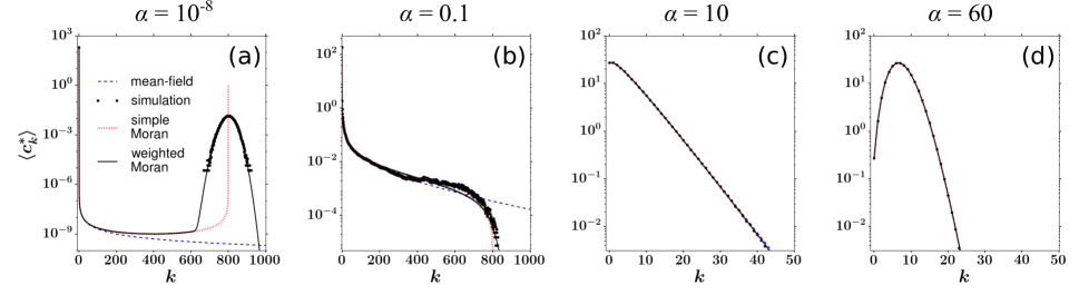
Figure 4: Simulated (black dots), mean-field (blue dashed), simple Moran (red hashes), and weighted Moran (black solid) approximations of $\langle c_{k}^{*}\rangle$ using logistic growth laws and the parameters $\mu=10,~{}p=20,~{}K=1600,~{}H=200$. Immigration rates used were (a) $\alpha=10^{-8}$, (b) $\alpha=0.1$, (c) $\alpha=10$, and (d) $\alpha=60$, as in Fig. 3. In (a) we show the prediction from a single Moran model of fixed size $N^{*}$. The weighted QSS Moran model approach (solid black curves) yields a very accurate approximation to the simulated values of $\langle c_{k}^{*}\rangle$ for all values of $\alpha$, including small $\alpha$ as shown in (a) and (b).

To calculate the covariance between $c_{k}^{*}$ and $c_{\ell}^{*}$ at QSS, we use the 2D ($q=2$) “continuum” solution given in Eq. (27) in the weighting in Eq. (29) in order to numerically compute Eq. (20). The covariances ${\rm cov}(c_{k}^{*},c_{\ell}^{*})\equiv\langle c_{k}^{*}c_{\ell}^{*}\rangle-\langle c_{k}^{*}\rangle\langle c_{\ell}^{*}\rangle$ with $\alpha=10^{-8}$, both from Monte-Carlo simulations and from our weighted Moran model approximation, are plotted in Fig. 5. The results provide insight on how the true dynamics for $\langle c_{k}^{*}\rangle$ in Eq. (5) differs from that of the mean-field description in Eq. (11).

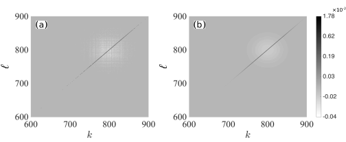
Figure 5: ${\rm cov}(c_{k},c_{\ell})$ from simulations (a) and from our calculations (b). Parameters are $\alpha=10^{-8},~{}\mu=10,~{}p=20,~{}K=1600,~{}H=200$. Only the interesting ranges of $k$ and $\ell$ close to $N^{*}\approx 800$ are shown. The pattern shows that large species counts are positively self-correlated (black line) but are negatively correlated with neighboring counts (white dots). The grey background shows no correlation between species counts of significantly different population levels. Greyscale values are shown on an exponential scale.

The large values (black line) along the diagonal $k=\ell$ corresponds to the peak in $\langle c_{k}^{*}\rangle$ [Eq. (20] is dominated by the $HP(n_{1}=k;t)$ term). White regions in the off-diagonal areas imply negative correlation between species counts of large neighboring sizes. In other words, whenever we observe a species with 800 individuals in a simulation at any fixed time $t$ (at QSS), we will probably not observe another species with 801 cells at the same time. Grey areas that are farther away (such as $k=\ell=600$) represent transient states of the system and have near-zero covariances.

IV.2 Other forms of global interactions

Since global interactions across all species mediate the breakdown of the mean-field approximation, we now investigate different forms of regulation imposed through the functions $r(N)$ and $\mu(N)$. To explore how the “stiffness” of different total population constraints affects the expected QSS species-count vector $\langle c_{k}^{*}\rangle$, we consider a simple Hill-type birth function with Hill coefficient 1:

$$r(N)=\frac{p_{2}K_{2}}{K_{2}+N},\qquad\mu(N)=\mu_{2}.$$ (31)

This form imposes a “softer” constraint on the total population $N$ than the logistic birth function. In order to compare the results with those of the logistic model in Subsection IV.1, we use the same values of $\alpha$ and $H$ and use $\mu_{2}=\mu,~{}p_{2}=p$ and $K_{2}=K-N^{*}$ where $N^{*}$ is the QSS population size obtained from the logistic model.

Another way to implement regulation is by keeping the birth rate constant but allowing the death rate to be population-dependent: parsons2008absorption

$$r(N)=r_{3},\qquad\mu(N)=\mu_{3}\left(1+\frac{N}{K_{3}}\right).$$ (32)

Again, we are interested in expected species counts near the same $N^{*}$ as in Subsection IV.1, we set $K_{3}=K,~{}r_{3}=r^{*},~{}\mu_{3}=\mu^{*}/(1+\frac{N^{*}}{K_{3}})$, where $r^{*}$ and $\mu^{*}$ are the QSS values of the birth and death rates used in the logistic model.

Note that both the alternative regulation models, the Hill-type model and the population-dependent death model, generate the same steady-state rates $r^{*}$ and $\mu^{*}$ at the same QSS total population size $N^{*}$ as in the logistic model. Thus, we can compare the expected species-counts from all three models on the same footing. Since the mean-field solution given in Eq. (11) depends only on $r^{*}$ and $\mu^{*}$, all three models yield identical mean-field solutions $\langle c_{k}^{*}\rangle$. Therefore, for not-too-small values of $\alpha$, for which mean-field solutions are accurate, all three models yield the same $\langle c_{k}^{*}\rangle$.

However, for small $\alpha$, where the mean-field approximation breaks down, we expect that the peak in $\langle c_{k}^{*}\rangle$ near $k=N^{*}$ will be quantitatively different among the three models. In Fig. 6, we set $\alpha=10^{-8}$ and plot the expected species count (from simulations and our weighted Moran model approximation) associated with each of the three models.

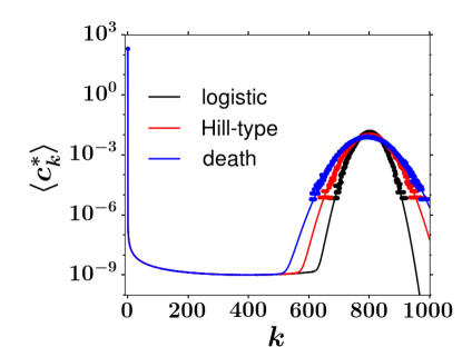
Figure 6: Comparison of $\langle c_{k}^{*}\rangle$ across the three regulation models, logistic (narrowest, black), Hill-type (intermediate, red), and population-dependent death (widest, blue). Simulations and results from the weighted Moran model approximations are shown. Here, the immigration rate is $\alpha=10^{-8}$ where the mean-field approximation is invalid. The other parameters are $\mu_{2}=10,~{}p_{2}=20,~{}H=200,K=1600,r_{3}=r^{*}$, and $\mu_{3}=\mu^{*}$.

Note that the peaks in $\langle c_{k}^{*}\rangle$ differ in their widths. In all examples, the underlying Moran models are identical and the differences originate in the different total-population distributions $P^{*}(N)$ across the three regulation models, as illustrated by the different “widths” of the peak near $N^{*}$. According to simulations and numerical solutions of our weighted Moran model, the peak widths corresponding to each regulatory model are ranked according to population-dependent death $>$ Hill-type $>$ logistic growth.

A wider peak in $\langle c_{k}^{*}\rangle$ can be associated with a “softer” total population constraint. As long as $f(N)$ on the right-hand side of Eq. (4) is a differentiable near $N^{*}$, we can define the regulatory “stiffness” by

$$|f_{*}^{\prime}|=-f_{*}^{\prime}\equiv\frac{\mbox{d}f(N)}{\mbox{d}N}\bigg{|}_{N^{*}}\in[0,+\infty).$$ (33)

Note that $f_{*}^{\prime}<0$ as long as $N^{*}$ is a locally stable point.

The larger $|f_{*}^{\prime}|$ is, the more likely the next event will be “compensatory” (e.g. a new birth increases the chance for the next event to be death). This stiffness can be also thought of as the curvature of a quadratic energy profile centered about $N^{*}$. The stiffnesses of our three examples (using $\alpha=10^{-8}$) are $|f_{*}^{\prime}|=|p-\mu-\frac{2p}{K}N^{*}|=10$ for logistic birth, $|f_{*}^{\prime}|=|p_{2}\frac{(N^{*})^{2}+2K_{2}N^{*}}{(N^{*}+K_{2})^{2}}-\mu_{2}|=5$ for Hill-type regulation, and $|f_{*}^{\prime}|=|r_{3}-\mu_{3}-\frac{2\mu_{3}}{K_{3}}N^{*}|=3.3$ for population-dependent death. These stiffness values are consistent with the progression of peak widths shown in Fig. 6.

We may extend our definition of the stiffness to cases where $f(N)$ is not differentiable. For example, the Moran model has an infinitely “stiff” constraint ($f^{\prime}_{*}=-\infty$) which “forces” an immediately death after a new birth. Nevertheless, as we have shown, even though a regulated BDI model may have much less sensitivity than the Moran model, the latter still provides insights on how such regulatory effects can induce an expected species count that exhibits a peak at $N^{*}$.

IV.3 Energy landscape and phase transition in the species-count distribution

In this section, we provide an interpretation of the failure of the mean-field equation [Eq. (11)] as a “phase-transition” in the statistics of populations. The full high-dimensional BDI model in QSS can be described by two processes: (1) evolution of individual species fractions via a Moran model that is equivalent across different regulation models, and (2) fluctuations of the total population size according to a QSS distribution that depends on the regulation model. Since the failure of the mean-field approach arises essentially from the emergence of a species that represents a large fraction of the whole population, we focus on the contribution of the Moran process.

A phase-transition can be conveniently visualized using a potential energy landscape $\phi$ as is widely used in population genetics and developmental biology wright1932roles ; Waddington1957 ; Sherrington1997 ; Arnold2001 ; Ao2009 ; Orr2009 ; xu2014two . Its recent development in the physics community has extended its application to quantitative and systems biology Ao2004 ; Qian2006 ; Wang2008 . Defined as a measure of “generalized energy”, its gradient indicates the direction of evolution of the system and its minima (potential wells) denote local stable states.

To simplify the math, we consider the $N\gg 1$ limit and use the continuum limit of the Moran model to find a continuum energy landscape $\phi(\{x_{1},x_{2},...\})$ such that $P^{*}_{\rm M}({\bf x})\propto e^{-\phi}$ satisfies Eq. (25) in steady-state. The shape of $\phi$ across $\{x_{1},x_{2},...\}$ characterizes the global stability of the model. Starting from the 1D version of Eq. (25) we have

$$A(x)=m^{*}\left(\frac{1}{H}-x\right),\quad B(x)=x(1-x),$$ (34)

which allow us to define the 1D energy function xu2014two

$$\phi(x) \equiv-N^{*}\int^{x}\frac{A(y)}{B(y)}+\ln B(x)$$

$$=\left(1-\frac{\alpha}{\mu^{*}}\right)\ln(x)+\left(1-\frac{\alpha(H-1)}{\mu^{*}}\right)\ln(1-x)$$

$$\equiv\frac{1}{H-1}\left[(H-1)-\frac{\alpha}{\alpha_{\rm c}}\right]\ln x+\left(1-\frac{\alpha}{\alpha_{\rm c}}\right)\ln(1-x).$$ (35)

Here, the parameter

$$\alpha_{\rm c}\equiv\frac{\mu^{*}}{H-1},$$ (36)

is a critical immigration rate that controls a “phase transition.” Eq. (36) is unambiguous when $\mu$ is constant. If the regulation arises from a population-dependent rate $\mu(N)$ as in Eq. (32), the critical immigration rate $\alpha_{\rm c}$ can be approximated by self-consistently solving $\alpha_{\rm c}=\mu(N^{*}(\alpha_{\rm c}))/(H-1)$.

When $P_{\rm M}^{*}(x)$ is normalisable, the energy function satisfies $\phi(x)\propto-\ln P_{\rm M}^{*}$. Since $\ln(0^{+})\to-\infty$ and $\ln(1)=0$, the shape of $\phi(x)$ is determined by the signs of the coefficients $H-1-\frac{\alpha}{\alpha_{\rm c}}$ and $1-\frac{\alpha}{\alpha_{\rm c}}$. Assuming $\alpha_{\rm c}>0$ (see Subsection IV.4 for the special case $\alpha_{\rm c}=0$), different regimes of the model can be delineated

• When $\alpha<\alpha_{\rm c}$, we have $\alpha<(H-1)\alpha_{\rm c}$ for $H\geq 2$. Two infinite minima in $\phi(x)$ emerge; one at $x=0$ and one at $x=1$. Associated with each minima is a basin of attraction as shown in Fig. 7(a). Even if all species start with a small fraction $x_{i}\ll 1$, one of them can eventually come to dominate by crossing to the attractive peak at $x=1$ causing a failure of the mean-field description. However, this transition is different from the usual stochastically-driven “escape” in statistical physics (see Discussion). When $\alpha$ is extremely small, the “extinction” state $x=0$ is approximately absorbing for each species and the mean-field approximation fails severely.

• When $\alpha=\alpha_{\rm c}$, $\alpha<(H-1)\alpha_{\rm c}$ for $H>2$. The potential $\phi(x)={H-2\over H-1}\ln x$ is monotonic and exhibits a global diverging minimum at $x=0$ and a global maximum at 1. The whole interval $[0,1]$ is a basin of attraction for $x=0$ as shown by Fig. 7(b). The energy away from $x=0$ is very flat and the severity of the failure of the mean-field approach is sensitive to $\alpha$ when it is near $\alpha_{\rm c}$.

• When $(H-1)\alpha_{\rm c}\geq\alpha>\alpha_{\rm c}$, the potential $\phi(x)$ has a diverging minimum at $x=0$ and a diverging maximum at $x=1$ as shown in Fig. 7(c). The mean-field approach is accurate in this regime.

• When $\alpha>(H-1)\alpha_{\rm c}$, there is a single finite minimum in $\phi(x)$ appearing at $x_{\rm min}=\frac{\alpha-\alpha_{\rm c}(H-1)}{\alpha H-2\alpha_{\rm c}(H-1)}$, which is close to $x=0$ when $H\gg 1$. The potential has diverging maxima at both $x=0$ and $x=1$ so the basin of attraction for $x_{\rm min}$ is the whole $[0,1]$ interval as shown by Fig. 7(d). The mean-field approach is accurate in this case.

Figure 7: Energy landscapes $\phi(x)$ as a function of $x=n/N^{*}$ for $\mu=10,~{}p=20,~{}K=1600,~{}H=200$ and different values of $\alpha$. (a) $\alpha=10^{-8}$ corresponding to Fig. 4(a), (b) $\alpha=\alpha_{\rm c}=10/199$, (c) $\alpha=0.1$, and (d) $\alpha=60$. The minimum at $x>0$ corresponds to the peak in $\langle c_{k}^{*}\rangle$ arising at $k>1$.

Physically, a small immigration rate $\alpha<\alpha_{\rm c}$ does not allow a dominant species to be replaced by new ones. When $\alpha>\alpha_{\rm c}$, the immigration frequency $\alpha H$ is larger that the rate of coarsening of the species counts thereby filling the system with new species and preventing any one species to dominate. Here, $\langle c_{k}^{*}\rangle$ is monotonically decreasing. At even larger $\alpha>(H-1)\alpha_{\rm c}$, immigration of each species is frequent enough that $\langle c_{k}^{*}\rangle$ becomes very broad and again develops an interior peak at $k\approx x_{\rm min}N^{*}$. The collapsing of $\langle c_{k}^{*}\rangle$ into a single species is reminiscent of the collapse of cluster size distributions in self-assembly under finite resources NUCLEATION1 .

IV.4 Resolving the effects of $\alpha$ and $H$

The energy landscape formulation provides a general way to visualize whether there is phase transition in the dynamics of an individual species. which can be applied to study how various parameter affect the model and generalized to various models. Equipped with the energy landscape, we can now examine the species populations as the intrinsic immigration rate $\alpha$ and the total number of species $H$ that can immigrate varied, keeping the total immigration rate, $\alpha H$, fixed. Varying $\alpha$ and $H$ in this way will not change the dynamics of the total population $N$ but will influence the dynamics of populations of individual species. This is readily shown by the different shapes of $\phi(x)$ as $\alpha$ and $H$ change. For example, let $\mu^{*}=0.33$. With $H=2,~{}\alpha=1$, the landscape exhibits a “most probable” species size maintained by high per-species immigration rate. However, if $H=200$ and $\alpha=0.01$, each species has a low immigration rate. The associated landscape $\phi(x)=0.97\ln x-5\ln(1-x)$ exhibits a unique potential well at $x=0$ as all species are driven small. We can also consider the limit $H\rightarrow\infty$ while keeping $\alpha H$ fixed. This limit approximates naive T cell generation by the thymus. While total thymic output $\alpha H$ is finite, there are theoretically $H>10^{15}$ different species (T-cell receptor sequences) that can be generated although only about $10^{6}-10^{8}$ different species survive lythe2016many . In any case, this large value of $H$ means that nearly every immigration is from a new, unrepresented species and $k=0$ is an absorbing boundary for all existing species. Species labels keep changing, but the distribution of $\langle c_{k}\rangle$ reaches a QSS. The energy landscape becomes (taking $\alpha\rightarrow 0$ in Eq. (35)) $\phi(x)\to\ln x+\left(1-\frac{\alpha H}{\mu^{*}}\right)\ln(1-x)$. There is always an potential well at $x=0$ while the dynamics near 1 depend on the sign of $\frac{\alpha H}{\mu^{*}}-1$.

Recall that if $\alpha<\alpha_{\rm c}$ the mean-field approximation to $\langle c_{k}\rangle$ fails. From Eq. (36), the critical value $\alpha_{\rm c}$ increases as $H$ decreases rendering the mean-field approximation invalid for a larger range of immigration rates. When $\alpha_{\rm c}\to 0$ (e.g. realized when $\mu^{*}\to 0$), Eq. (35) no longer has a valid form because birth would need to be negative ($N^{*}>K$) in order to balance immigration. Nonetheless, we can multiply the landscape function by a constant $\mu^{*}$ without affecting its ability to qualitatively characterize and classify the dynamics of the system. We then take the limit $\mu^{*}\rightarrow 0$ and get $\phi\propto-\alpha\ln(x)-\alpha(H-1)\ln(1-x)$, which always has a unique minimum between $(0,1)$, corresponding to Fig. 7(d).

V Discussion and Summary

In our analysis, the non-mean-field behavior of the expected clone abundances are mediated by global regulation mechanisms that act uniformly across all clones. Such population-dependent interactions break independence between clones, are difficult to model, and consequently have been rarely discussed in the context of species diversity volkov2005density . Empirical studies have focused on the small-to-intermediate range of $k$, where the distribution $\langle c_{k}^{*}\rangle$ is well approximated by the mean-field model (Eq. (11)) as seen in Figs. 3 and 4. In another study, Parsons et al. parsons2008absorption considered a neutral and quasi-neutral birth-death model with carrying capacity but focussed on the mean fixation time of any species rather than species counts. However, they find that fluctuations in the total population do not affect fixation times of neutral species which is consistent with our finding that a fixed-population Moran process can be used to accurately construct the fractions $\frac{n_{1}}{N}$ of any species in our BDI model. To our knowledge, the failure of predicting a large-size clone by Eq. (11) has not been explicitly discussed in detail.

In many contexts such as stem or progenitor cells in a bone marrow niche, or multiple species competing for common resources, the observation of one or a few large clones or high population species is often naturally attributed to selection (differences in growth or death rates). This largest “outlier” clone can contain most of the population and be biologically more important than all other smaller clones/species in the organism/community. Our results show that a simpler mechanism may arise from slow immigration into a neutral birth-death process with regulation, providing an initial “null hypothesis” for selection. Otherwise, one may incorrectly argue that the existence of such a singular outlier clone suggests a species selection effect.

To quantitatively understand the regulated multispecies BDI process, we showed that an often-used mean-field approximation captures the expected steady-state species counts at low populations, but completely misses a possible peak in the species abundance near the population supported by a general regulated birth-death-immigration process. This peak arises only when the immigration rate decreases below a threshold value.

To develop a theory that approximates the clone abundance distribution accurately in all parameter regimes, we then mapped the $q^{\rm th}$ moment of the species abundance distribution $c_{k}$ to a $(q+1)$-dimensional cell-count BDI model, which was then approximated by weighting over $q$-dimensional Moran models of different system size. The expected distribution and covariances of species counts were accurately calculated in parameter regimes in which the mean-field approximations break down. By exploiting the concept of energy landscapes, we analytically describe a phase transition in the dynamics which explains the failure of the mean-field approach in the original model. Our analysis shows that global (inter-species) carrying capacity, when combined with a random sampling mechanism, generates a genetic-drift-like effect ewens2012mathematical in a Moran model that ultimately destroys the universal power-law distribution of $c_{k}$.

In Eq. (5), dynamics of any $\langle c_{k}^{*}\rangle$ are controlled by $r(N)$, where $N\equiv\sum_{\ell}\ell c_{\ell}$. It involves contributions from all clone populations $\ell=0,1,2,...,k,...$ Recall that in many classical scenarios the relative strengths of these effects on the $k^{\rm th}$ component decay with distance $|k-\ell|$. For example, in the constant-rate BDI model, only $c_{k\pm 1}$ and $c_{k}$ affect the dynamics of $c_{k}$. Here, however, the contribution from $c_{\ell}$ is proportional to the index $\ell$ itself instead of on $|k-\ell|$. This is a type of “long-range” interaction or long-distance coupling arise in theoretically challenging contexts in different areas morchio1987mathematical ; takayama2012cooperative ; sanyal2012long ; chen2016long . Thus, the structure of $\langle c_{k}^{*}\rangle$ according to Eq. (5) can no longer be approximated by a simple monotonic form as is shown in Fig. (5) where correlations between large $k$ and its neighboring states $k\pm 1$ are negative.

To effectively find higher moments of species counts in QSS, higher-dimensional Moran models can be used to construct the related QSS cell-count distributions. Diffusion approximations to high-dimensional Moran models provide convenient analytic-form steady-state distributions ewens1963numerical ; aalto1989moran ; baxter2007exact . However, the boundary values of $P^{*}_{\rm M}({\bf x})$ in the diffusion approximation may not accurately approximate those from the discrete Moran model, especially in higher dimensions. For example, when $N^{*}m^{*}\ll 1$ in Eq. (27), $P_{\rm M}(x_{i}=0)=+\infty$ but $P_{\rm M}(x_{i}=\frac{1}{N})\approx 0$. Near the boundary, $P_{\rm M}(0<x<\frac{1}{N})$ generally changes in a highly non-linear fashion. Only with extremely large $N$ do the probability distributions of the discrete and continuous Moran models match well doering2005extinction ; kessler2007extinction . Nevertheless, our result in Fig. 5 is accurate because the region of interest is far away from the boundaries. Moreover, the second moment $\langle(c_{k}^{*})^{2}\rangle$ in Eq. (20) turns out to be dominated by the first-moment term $H\langle c_{k}^{*}\rangle$ which was calculated based on the exact discrete solution in Eq. (24).

It is worth noting that the initial establishment of the large clone $i$, denoted by the transition $x_{i}\approx 0\rightarrow x_{i}\approx 1$, is different from traditional scenarios where clone $i$ randomly crosses the energy barrier near $x=0.5$ and “escapes” to the other attractive basin. Here, the potential energy profile corresponds to QSS in which there are many different clones $j$ starting with small fractions $x_{j}\approx 0$. One of these small clones eventually replaces the dominating clone $i$ ($x_{j}\approx 1$). The waiting time for such replacement event was obtained by xu2014two as $T_{\rm r}\sim\mathcal{O}(\frac{N^{*}}{\alpha(H-1)})$, a much longer time than the waiting time $T_{2}\sim\mathcal{O}(\frac{N^{*}}{\mu^{*}})$ (see Appendix C) for the establishment of the first dominant clone in our BDI regulated model under $\alpha(H-1)\ll\mu^{*}$.

Future improvements to our analysis include more accurately determining steady-state solutions of the higher dimensional Moran models, especially near the boundaries and extending our approaches to time-dependent approximations. To better distinguish our neutral mechanism from true selection, a careful analysis of heterogeneous populations should be explored to determine how random dominance from neutral regulation might be balanced by selection in the form of heterogeneous growth, death, and immigration parameters.

VI Acknowledgments

This work was supported in part by grants from the NSF (DMS-1516675 and DMS-1814364) and the Army Research Office (W911NF-18-1-0345).

Mathematical Appendices

Appendix A Cell-count Master equation for $P(n_{1},...,n_{i},...,n_{H};t)$

The high-dimensional master equation obeyed by the full multispecies distribution reads

$${\partial P({\bf n};t)\over\partial t}=\alpha\sum_{i=1}^{H}P(n_{1},...,n_{i-1},n_{i}-1,n_{i+1},...,n_{H})-P({\bf n})]$$

$$\qquad+\sum_{i=1}^{H}\left[r(N-1)(n_{i}-1)P(n_{1},...,n_{i}-1,...,n_{H})-r(N)n_{i}P({\bf n})\right]$$

$$\qquad+\sum_{i=1}^{H}\left[\mu(N+1)(n_{i}+1)P(n_{1},...,n_{i}+1,...,n_{H})-\mu(N)n_{i}P({\bf n})\right],$$ (37)

where $N\equiv\sum_{i=1}^{H}n_{i}$.

Appendix B Dynamical equations for $\langle c_{k}(t)\rangle$

Define $P({\bf c};t)$ as the probability of observing the configuration ${\bf c}=\{c_{0},c_{1},c_{2},...\}$ at a specific time $t$. Under constant immigration and population-regulated birth and death rates, the evolution of the full probability distribution satisfies the master equation

$$\frac{\partial P({\bf c};t)}{\partial t}=-\sum_{k=0}^{\infty}[\alpha+(\mu(N)+r(N))k]c_{k}P({\bf c})$$

$$\qquad\qquad\qquad+\sum_{k=0}^{\infty}(c_{k+1}+1)(k+1)\mu(N+1)P(\{...,c_{k}-1,c_{k+1}+1,...\})$$

$$\qquad\qquad\qquad+\sum_{k=0}^{\infty}(c_{k}+1)(\alpha+kr(N-1))P(\{...,c_{k}+1,c_{k+1}-1,...\}).$$ (38)

Without loss of generality, let us assume constant $\mu,~{}\alpha$ but regulated $r=r(N)=r(\sum_{k=1}^{\infty}kc_{k})$. The expected clone count is

$$\langle c_{\ell}(t)\rangle=\sum_{c_{\ell}=0}^{H}c_{\ell}P(c_{\ell};t)=\sum^{H}_{c_{0}=0}\sum^{H}_{c_{1}=0}...\sum_{c_{k}=0}^{H}...~{}c_{\ell}P(c_{0},c_{1},...,c_{\ell-1},c_{\ell},c_{\ell+1},...;t).$$ (39)

Substituting Eq. (38) into Eq. (39), we obtain

$$\frac{\mbox{d}\langle c_{\ell}(t)\rangle}{\mbox{d}t}=\sum^{H}_{c_{0}=0}\sum^{H}_{c_{1}=0}...\sum_{c_{k}=0}^{H}...~{}c_{\ell}\frac{\partial P(c_{0},c_{1},...,c_{k-1},c_{k},c_{k+1},...;t)}{\partial t}$$

$$=\sum^{H}_{c_{0}=0}\sum^{H}_{c_{1}=0}...\sum_{c_{k}=0}^{H}...~{}c_{\ell}\bigg{\{}\sum_{k=0}^{\infty}-[\alpha+(\mu+r(N))k]c_{k}P(c_{0},c_{1},...,c_{k-1},c_{k},c_{k+1},...)$$

$$\qquad+\sum_{k=0}^{\infty}(c_{k+1}+1)[(k+1)\mu]P(c_{0},c_{1},...,c_{k-1},c_{k}-1,c_{k+1}+1,...)$$

$$\qquad+\sum_{k=0}^{\infty}(c_{k}+1)[\alpha+kr(N-1)]P(c_{0},c_{1},...,c_{k-1},c_{k}+1,c_{k+1}-1,...)\bigg{\}}.$$ (40)

By collecting only terms in Eq. (40) that involve $r(N)$, we obtain two summations

$$S_{1}+S_{2}\equiv-\sum^{H}_{c_{0}=0}\sum^{H}_{c_{1}=0}...\sum_{c_{k}=0}^{H}...~{}c_{\ell}\sum_{k=0}^{\infty}r(N)kc_{k}P(c_{0},c_{1},...,c_{k-1},c_{k},c_{k+1},...)$$

$$\qquad+\sum^{H}_{c_{0}=0}\sum^{H}_{c_{1}=0}...\sum_{c_{k}=0}^{H}...~{}c_{\ell}\sum_{k=0}^{\infty}r(N-1)k(c_{k}+1)P(c_{0},c_{1},...,c_{k-1},c_{k}+1,c_{k+1}-1,...).$$

Consider the contribution of the $k^{\rm th}$ terms in both summations:

• When $k<\ell-1$ or $k\geq\ell+1$, the $k^{\rm th}$ term of $S_{1}$ becomes

  $$-\sum^{H}_{c_{0}=0}\sum^{H}_{c_{1}=0}...\sum_{c_{k}=0}^{H}...~{}c_{2}r(N)(k-1)c_{k-1}P(c_{0},c_{1},c_{2},...,c_{k},...)$$ (41)

  and $k^{\rm th}$ term of $S_{2}$ becomes

  $$\sum^{H}_{c_{0}=0}...\sum_{c_{k-1}=0}^{H}\sum_{c_{k}=0}^{H}...~{}c_{\ell}r(N-1)(k-1)(c_{k-1}+1)P(c_{0},c_{1},...,c_{k-1}+1,c_{k}-1,...)$$

  $$=\sum^{H}_{c_{0}=0}...\sum_{c_{k-1}=0}^{H}\sum_{c_{k}=0}^{H-1}...~{}c_{\ell}r(N)(k-1)c_{k-1}P(c_{0},c_{1},c_{2},...,c_{k-1},c_{k},...)$$

  $$=\sum^{H}_{c_{0}=0}...\sum_{c_{k-1}=0}^{H}\sum_{c_{k}=0}^{H}...~{}c_{\ell}r(N)(k-1)c_{k-1}P(c_{0},c_{1},c_{2},...,c_{k-1},c_{k},...).$$ (42)

  The last equality holds since $P(c_{k}=H)=0$ due to the constraint that if $c_{k}=H$, then all other $c_{m\neq k}=0$.

• When $k=\ell-1$, the $k^{\rm th}$ term of $S_{1}$ is

  $$-\sum^{H}_{c_{0}=0}...\sum_{c_{\ell-1}=0}^{H}\sum_{c_{\ell}=0}^{H}...~{}c_{\ell}r(N)(\ell-1)c_{\ell-1}P(c_{0},c_{1},c_{2},...,c_{k},...)$$ (43)

  and the $k^{\rm th}$ term of $S_{2}$ is

  $$\sum^{H}_{c_{0}=0}...\sum_{c_{\ell-1}=0}^{H}\sum_{c_{\ell}=0}^{H}...~{}c_{\ell}r(N-1)(\ell-1)(c_{\ell-1}+1)P(c_{0},c_{\ell-1}+1,c_{\ell}-1,c_{3},...,c_{k},...)$$

  $$\qquad=\sum^{H}_{c_{0}=0}...\sum_{c_{\ell-1}=0}^{H}\sum_{c_{\ell}=0}^{H-1}...~{}(c_{\ell}+1)r(N)c_{\ell-1}P(c_{0},c_{1},c_{2},c_{3},...,c_{k},...)$$

  $$\qquad=\sum^{H}_{c_{0}=0}...\sum_{c_{\ell-1}=0}^{H}\sum_{c_{\ell}=0}^{H}...~{}(c_{\ell}+1)r(N)c_{\ell-1}P(c_{0},c_{1},c_{2},c_{3},...,c_{k},...).$$ (44)

  The two terms sum to

  $$\sum^{H}_{c_{0}=0}\sum^{H}_{c_{1}=0}\sum_{c_{2}=0}^{H}...\sum_{c_{k}=0}^{H}...~{}r(N)c_{\ell-1}P(c_{0},c_{1},c_{2},...,c_{k},...)=\langle r(N)c_{\ell-1}\rangle.$$ (45)

• When $k=\ell$, the $k^{\rm th}$ term of $S_{1}$ is

  $$-\sum^{H}_{c_{0}=0}...\sum_{c_{\ell-1}=0}^{H}\sum_{c_{\ell}=0}^{H}...~{}c_{\ell}r(N)\ell c_{\ell}P(c_{0},c_{1},c_{2},...,c_{k},...)$$ (46)

  while the $k^{\rm th}$ term of $S_{2}$ is

  $$\sum^{H}_{c_{0}=0}...\sum_{c_{\ell}=0}^{H}\sum_{c_{\ell+1}=0}^{H}...~{}c_{\ell}r(N-1)\ell(c_{\ell}+1)P(c_{0},c_{1},c_{\ell}+1,c_{\ell+1}-1,...,c_{k},...)$$

  $$\qquad=\sum^{H}_{c_{0}=0}...\sum_{c_{\ell}=0}^{H}\sum_{c_{\ell+1}=0}^{H-1}...~{}(c_{\ell}-1)r(N)\ell c_{\ell}P(c_{0},c_{1},c_{2},...,c_{k},...)$$

  $$\qquad=\sum^{H}_{c_{0}=0}...\sum_{c_{\ell}=0}^{H}\sum_{c_{\ell+1}=0}^{H}...~{}(c_{\ell}-1)r(N)\ell c_{\ell}P(c_{0},c_{1},c_{2},...,c_{k},...).$$ (47)

  These two terms sum to

  $$\sum^{H}_{c_{0}=0}...\sum_{c_{\ell}=0}^{H}\sum_{c_{\ell+1}=0}^{H}...r(N)\ell(-c_{\ell})P(c_{0},c_{1},c_{2},...,c_{k},...)=-\ell\langle r(N)c_{\ell}\rangle.$$ (48)

Summarizing, terms that involve $r(N)$ in Eq. (40) are simplified as $(\ell-1)\langle r(N)c_{\ell-1}\rangle-\ell\langle r(N)c_{\ell}\rangle$. Terms involving $\alpha$ and $\mu$ can be similarly obtained if they are regulated by $N$. Together, Eq. (40) becomes

$${\mbox{d}\langle c_{\ell}\rangle\over\mbox{d}t}=\alpha(\langle c_{\ell-1}\rangle-\langle c_{\ell}\rangle)+\langle r(N)\left[(\ell-1)c_{\ell-1}-\ell c_{\ell}\right]\rangle+\langle\mu(N)\left[(\ell+1)c_{\ell+1}-\ell c_{\ell}\right]\rangle.$$ (49)

Appendix C Multi-timescale dynamics of $N(t)$ and $c_{k}(t)$

For simplicity, we first discuss the model with no immigration ($\alpha=0$) and a large carrying capacity $K$. In this limit, $N^{*}=(1-\frac{\mu}{p})K\sim\mathcal{O}(K^{-1})$. The deterministic Eq. (4) gives quite a good approximation for the typical dynamics for $N$ in its first phase of evolution as $N(t)$ quickly approaches its QSS value $\langle N^{*}\rangle$. To estimate this timescale, one can integrate $\frac{\mbox{d}N}{\mbox{d}t}$ in Eq. (13) under $\alpha=0$ to find $\langle N(t)\rangle=\frac{\langle N^{*}\rangle N_{0}}{N_{0}+e^{-(p-\mu)t}(\langle N^{*}\rangle-N_{0})}$. Thus $N$ approaches $\langle N^{*}\rangle$ in a characteristic timescale $\mathcal{O}(\frac{1}{p-\mu})$.

As $N$ approaches $\langle N^{*}\rangle$, $r(N)$ also approaches $r(\langle N^{*}\rangle)\equiv r^{*}$, allowing $\langle c_{k}\rangle$ to approach its QSS value $\langle c_{k}^{*}\rangle$ which has a high peak at $k=0$ and a small peak at $k\approx\langle N^{*}\rangle$. Although this peak is small, the number of individuals in this clone, $kc_{k\approx\langle N^{*}\rangle}$ can comprise nearly the entire population. This configuration is associated with a single large-size clone that persists after the disappearance of all other $H-1$ clones. If we define the number of living clones (or “species richness”)

$$R\equiv\sum_{k=1}^{\infty}c_{k},$$ (50)

this “coarsening” or “fixation” process [46] decreases $R$ from its initial value $H$ to 1 in finite time. We define the waiting time for such a fixation to take place as $T_{1}$. Since fixation is most relevant to changes of fractions of clones, we study the problem in a Moran model. In a standard textbook such as [46], the mean time for the $i^{\rm th}$ clone to fix (conditioned on its fixation) is $T_{\rm fix}(i)\approx-\frac{N^{*}}{\mu}\frac{N(0)-n_{i}(0)}{n_{i}(0)}\ln\left[1-\frac{n_{i}(0)}{N(0)}\right]$. The expected time until any arbitrary clone’s fixation is then calculated by averaging each clone’s fixation times over its its probability of fixation ($P_{\rm fix}(i)=x_{i}(0)$) as $T_{\rm c}=\sum_{i}T_{\rm fix}(i)P_{\rm fix}(i)\approx\frac{N^{*}}{\mu}$.

The last clone, which is just the total population, is stabilized to $N^{*}$ by the regulatory effect of $f(N)$. It fluctuates around $N^{*}$ for an exponentially long time. The variance (“width”) of such fluctuation near $N^{*}$ can be calculated by invoking the full stochastic model Eq. (3) which leads to the solution $P^{*}(N)$ in Eq. (28). The fact that $P^{*}(0)\neq 0$ (although it is typically exponentially small) allows for a finite probability that $N$ may incur a large deviation to the absorbing boundary $N=0$, resulting in extinction of the total population [54]. The expected time to extinction of the total population is $T_{\rm ext}=\sum_{m=1}^{n}a_{m}$ where $a_{m}=\frac{1}{\mu m}+\sum_{j=1}^{\infty}\frac{1}{\mu(m+j)}\prod_{i=1}^{j}\frac{r_{m+i-1}}{\mu}$ [53]. The asymptotic approximation $T_{\rm ext}\sim\mathcal{O}(e^{\langle N^{*}\rangle})$ indicate a very long timescale for extinction, well after QSS limit of $\langle c_{k}^{*}\rangle$ is approached.

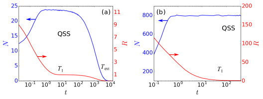
Figure 8: Simulations of the multi-timescale dynamics of a small (a) and a large (b) system. Common parameters are $\mu=10,~{}p=20$. Different parameters are $K=50,~{}H=11,~{}\alpha=0$ for (a) and $K=1600,~{}H=200,~{}\alpha=10^{-8}$ for (b).

In Fig. 8, we plot simulations of the dynamics of both $N$ and $R$ under two different sets of parameters. Values of $\alpha$ are set to be extremely small or 0. Fig. 8(a) shows that $N$ reaches $N^{*}\approx 25$ within 1 unit of time and remains stable over approximately $10^{2}$ before extinction. For $\alpha=0$, we can identify a QSS within the time period $T_{1}<t<T_{\rm ext}$. Fig. 8(b) incorporates a small immigration $\alpha=10^{-8}$ so that $N=0$ is technically no longer an absorbing boundary. Nonetheless, for extremely small $\alpha HT_{\rm ext}\ll 1$, the dynamics are similar to the $\alpha=0$ case (Fig. 7(a)) since the inter-immigration times $1/(\alpha H)$ are longer than the extinction time of the whole population.

Appendix D Moments

The first moment of ${\bf c}$ is readily obtained by invoking its definition in Eq. (1) as

$$\langle c_{k}\rangle=\sum_{{\bf n}}[\mathds{1}(n_{1},k)+\mathds{1}(n_{2},k)+...+\mathds{1}(n_{H},k)]P({\bf n})=H\sum_{{\bf n}}\mathds{1}(n_{1},k)P({\bf n})=HP(k)$$

The second moment, when $k\neq\ell$, is obtained as

$$\langle c_{k}c_{l}\rangle=\sum_{{\bf n}}[\mathds{1}(n_{1},k)+...+\mathds{1}(n_{H},k)][\mathds{1}(n_{1},\ell)+...+\mathds{1}(n_{H},\ell)]P({\bf n})$$

$$\qquad=\sum_{{\bf n}}\sum_{i=1}^{H}\mathds{1}(n_{i},k)[\mathds{1}(n_{1},\ell)+...+\mathds{1}(n_{H},\ell)]P({\bf n})$$

$$\qquad=H\sum_{{\bf n}}\sum_{j\neq 1}\mathds{1}(n_{1},k)\mathds{1}(n_{j},\ell)P({\bf n})=H(H-1)\sum_{{\bf n}}\mathds{1}(n_{1},k)\mathds{1}(n_{2},\ell)P({\bf n})$$

$$\qquad=H(H-1)P(k,\ell).$$

When $k=\ell$, we have

$$\langle c_{k}c_{k}\rangle=\sum_{{\bf n}}[\mathds{1}(n_{1},k)+...+\mathds{1}(n_{H},k)][\mathds{1}(n_{1},k)+...+\mathds{1}(n_{H},k)]P({\bf n})$$

$$\qquad=H(H-1)P(k,k)+H\sum_{{\bf n}}\mathds{1}(n_{1},k)\mathds{1}(n_{1},k)P({\bf n})$$

$$\qquad=H(H-1)P(k,k)+HP(k).$$

The third moment, when $k\neq\ell\neq m$, is obtained as

$$\langle c_{k}c_{\ell}c_{m}\rangle=\sum_{{\bf n}}[\mathds{1}(n_{1},k)+...+\mathds{1}(n_{H},k)][\mathds{1}(n_{1},\ell)+...+\mathds{1}(n_{H},\ell)][\mathds{1}(n_{1},m)+...+\mathds{1}(n_{H},m)]P({\bf n})$$

$$\qquad=\sum_{{\bf n}}\sum_{i=1}^{H}\mathds{1}(n_{i},k)[\mathds{1}(n_{1},\ell)+...+\mathds{1}(n_{H},\ell)][\mathds{1}(n_{1},m)+...+\mathds{1}(n_{H},m)]P({\bf n})$$

$$\qquad=H\sum_{{\bf n}}\mathds{1}(n_{1},k)\sum_{i\neq 1}\mathds{1}(n_{i},\ell)\sum_{j\neq 1,i}\mathds{1}(n_{j},m)P({\bf n})$$

$$\qquad=H(H-1)(H-2)P(k,\ell,m).$$

When $k=\ell\neq m$, we have

$$\langle c_{k}^{2}c_{m}\rangle=H(H-1)(H-2)P(k,k,m)+\sum_{{\bf n}}[\mathds{1}(n_{1},k)+...+\mathds{1}(n_{H},k)][\mathds{1}(n_{1},m)+...+\mathds{1}(n_{H},m)]$$

$$\qquad=H(H-1)(H-2)P(k,k,m)+H(H-1)P(k,m).$$

And finally when $k=\ell=m$, we obtain

$$\langle c_{k}^{3}\rangle=H(H-1)(H-2)P(k,k,k)+H(H-1)P(k,k)+\sum_{{\bf n}}[\mathds{1}(n_{1},k)+...+\mathds{1}(n_{H},k)]$$

$$\qquad=H(H-1)(H-2)P(k,k,k)+H(H-1)P(k,k)+HP(k).$$

Appendix E Diffusion approximation by the Taylor expansion

For notational simplicity, we replace $x_{1}$ with continuous variables $x$ and neglect the subscript “M” in the Moran model probability $P_{\rm M}$ in the rest of this subsection. Letting $\varepsilon=\frac{1}{N^{*}}\rightarrow 0$ ($N^{*}\rightarrow\infty$) in Eq. (21), we expand the transition rates to second order in $\varepsilon$:

$$\omega_{12}(x-\varepsilon)P(x-\varepsilon)\approx(\omega_{12}P)-\varepsilon(\omega_{12}P)^{\prime}+\frac{\varepsilon^{2}}{2}(\omega_{12}P)^{\prime\prime},$$ (51)

$$\omega_{21}(x+\varepsilon)P(x+\varepsilon)\approx(\omega_{21}P)+\varepsilon(\omega_{21}P)^{\prime}+\frac{\varepsilon^{2}}{2}(\omega_{21}P)^{\prime\prime}.$$ (52)

Substituting them into Eq. (21), considering $\omega_{12}(x)=\alpha(1-x)+r^{*}N^{*}x(1-x),~{}\omega_{21}(x)=\alpha(H-1)x+r^{*}N^{*}x(1-x)$ in Eq. (22), and canceling out terms, we obtain (when $\alpha H\ll r^{*}N^{*}$)

$${\rm RHS}\approx-\varepsilon[(\omega_{12}-\omega_{21})P]^{\prime}+\frac{\varepsilon^{2}}{2}[(\omega_{12}+\omega_{21})P]^{\prime\prime}$$

$$\qquad=-\frac{\alpha H}{N^{*}}\frac{\partial}{\partial x}\left(\frac{1}{H}-x\right)P+\frac{1}{2(N^{*})^{2}}\frac{\partial^{2}}{\partial x^{2}}[\alpha(1-x)+\alpha(H-1)x+2r^{*}N^{*}x(1-x)]P$$

$$\qquad\approx-\frac{\alpha H}{N^{*}}\frac{\partial}{\partial x}\left(\frac{1}{H}-x\right)P+\frac{r^{*}N^{*}}{(N^{*})^{2}}\frac{\partial^{2}}{\partial x^{2}}x(1-x)P$$

$$\qquad\approx\mu^{*}N^{*}\left[-\frac{1}{N^{*}}\frac{\partial}{\partial x}m^{*}\left(\frac{1}{H}-x\right)P_{\rm M}(x)+\frac{1}{(N^{*})^{2}}\frac{\partial^{2}}{\partial x^{2}}x(1-x)P_{\rm M}(x)\right]$$ (53)

where $m^{*}=\frac{\alpha H}{\mu^{*}N^{*}}$ is the fraction of birth that comes from immigration.

For the 2D Moran model, we have

$$\frac{\partial P(x_{1},x_{2})}{\partial t}=(\omega_{21}P)(x_{1}+\varepsilon,x_{2}-\varepsilon)+(\omega_{31})P(x_{1}+\varepsilon,x_{2})+(\omega_{12}P)(x_{1}-\varepsilon,x_{2}+\varepsilon)$$

$$\qquad+(\omega_{32}P)(x_{1},x_{2}+\varepsilon)+(\omega_{13}P)(x_{1}-\varepsilon,x_{2})+(\omega_{23}P)(x_{1},x_{2}-\varepsilon)$$

$$\qquad-[(\omega_{21}+\omega_{31}+\omega_{21}+\omega_{32}+\omega_{13}+\omega_{23})P](x_{1},x_{2})$$ (54)

where

$$\omega_{21}=\alpha x_{1}+r^{*}N^{*}x_{2}x_{1},\qquad\omega_{31}=\alpha(H-2)x_{1}+r^{*}N^{*}x_{3}x_{1},$$ (55)

$$\omega_{12}=\alpha x_{2}+r^{*}N^{*}x_{1}x_{2},\qquad\omega_{32}=\alpha(H-2)x_{2}+r^{*}N^{*}x_{3}x_{2},$$ (56)

$$\omega_{13}=\alpha x_{3}+r^{*}N^{*}x_{1}x_{3},\qquad\omega_{23}=\alpha x_{2}+r^{*}N^{*}x_{3}x_{2}.$$ (57)

Invoking the 2D Taylor expansion on Eq. (54), we obtain terms like

$$(\omega_{21}P)(x_{1}+\varepsilon,x_{2}-\varepsilon)\approx(\omega_{21}P)+\varepsilon\left[\frac{\partial(\omega_{21}P)}{\partial x_{1}}-\frac{\partial(\omega_{21}P)}{\partial x_{2}}\right]$$

$$\qquad\qquad\qquad\qquad\qquad\qquad+\frac{\varepsilon^{2}}{2}\left[\frac{\partial^{2}(\omega_{21}P)}{\partial x_{1}^{2}}-2\frac{\partial(\omega_{21}P)}{\partial x_{1}}\frac{\partial(\omega_{21}P)}{\partial x_{2}}+\frac{\partial^{2}(\omega_{21}P)}{\partial x_{2}^{2}}\right].$$

The right-hand side of Eq. (54) is thus approximated by

$${\rm RHS}\approx\varepsilon\left[\frac{\partial(\omega_{21}P)}{\partial x_{1}}-\frac{\partial(\omega_{21}P)}{\partial x_{2}}\right]+\frac{\varepsilon^{2}}{2}\left[\frac{\partial^{2}(\omega_{21}P)}{\partial x_{1}^{2}}-2\frac{\partial^{2}(\omega_{21}P)}{\partial x_{1}\partial x_{2}}+\frac{\partial^{2}(\omega_{21}P)}{\partial x_{2}^{2}}\right]$$

$$\qquad\qquad+\left[\varepsilon\frac{\partial(\omega_{31}P)}{\partial x_{1}}+\frac{\varepsilon^{2}}{2}\frac{\partial^{2}(\omega_{31}P)}{\partial x_{1}^{2}}\right]+\left[\varepsilon\frac{\partial(\omega_{32}P)}{\partial x_{2}}+\frac{\varepsilon^{2}}{2}\frac{\partial^{2}(\omega_{32}P)}{\partial x_{2}^{2}}\right]$$

$$\qquad\qquad+\varepsilon\left[-\frac{\partial(\omega_{12}P)}{\partial x_{1}}+\frac{\partial(\omega_{12}P)}{\partial x_{2}}\right]+\frac{\varepsilon^{2}}{2}\left[\frac{\partial^{2}(\omega_{12}P)}{\partial x_{1}^{2}}-2\frac{\partial^{2}(\omega_{12}P)}{\partial x_{1}\partial x_{2}}+\frac{\partial^{2}(\omega_{12}P)}{\partial x_{2}^{2}}\right]$$

$$\qquad\qquad+\left[-\varepsilon\frac{\partial(\omega_{13}P)}{\partial x_{1}}+\frac{\varepsilon^{2}}{2}\frac{\partial^{2}(\omega_{13}P)}{\partial x_{1}^{2}}\right]+\left[-\varepsilon\frac{\partial(\omega_{23}P)}{\partial x_{2}}+\frac{\varepsilon^{2}}{2}\frac{\partial^{2}(\omega_{23}P)}{\partial x_{2}^{2}}\right]$$

$$\qquad=\varepsilon\left[\frac{\partial}{\partial x_{1}}(\omega_{21}+\omega_{31}-\omega_{12}-\omega_{13})P+\frac{\partial}{\partial x_{2}}(\omega_{12}+\omega_{32}-\omega_{21}-\omega_{23})P\right]$$

$$+\frac{\varepsilon^{2}}{2}\left[\frac{\partial^{2}}{\partial x_{1}^{2}}(\omega_{21}+\omega_{31}+\omega_{12}+\omega_{13})P+\frac{\partial^{2}}{\partial x_{2}^{2}}(\omega_{12}+\omega_{32}+\omega_{21}+\omega_{23})P-2\frac{\partial^{2}}{\partial x_{1}\partial x_{2}}(\omega_{12}+\omega_{21})P\right]$$

$$\qquad=\mu^{*}N^{*}\left[-\frac{1}{N^{*}}\sum_{i=1}^{2}\frac{\partial A_{i}({\bf x})P({\bf x})}{\partial x_{i}}+\frac{1}{(N^{*})^{2}}\sum_{i=1}^{2}\sum_{j=1}^{2}\frac{\partial^{2}B_{ij}({\bf x})P({\bf x})}{\partial x_{i}\partial x_{j}}\right]$$ (58)

where

$$A_{i}({\bf x})=\sum_{j=1}^{2}m^{*}(Q_{i}-x_{i}),~{}~{}B_{ii}({\bf x})=x_{i}(1-x_{i}),~{}~{}B_{ij}({\bf x})=-x_{i}x_{j}~{}(i\neq j).$$ (59)

The last step of Eq. (58) involves calculations based on Eqs. (55-57) and the assumption $m^{*}\ll 1$. For example,

$$\omega_{12}-\omega_{21}+\omega_{13}-\omega_{31}=\alpha(1-x_{1})-\alpha Hx_{1}=\alpha H\left(\frac{1}{H}-x_{1}\right)\equiv\mu^{*}N^{*}\cdot m^{*}(Q_{1}-x_{1})$$

$$\omega_{21}+\omega_{31}=\alpha(H-1)x_{1}+r^{*}N^{*}x_{1}(x_{2}+x_{3})\approx\mu^{*}N^{*}\cdot x_{1}(1-x_{1}).$$

$$\omega_{12}+\omega_{13}=\alpha(1-x_{1})+r^{*}N^{*}x_{1}(1-x_{1})\approx r^{*}N^{*}x_{1}(1-x_{1})$$ (60)

References

- [1] Veronika I. Zarnitsyna, Brian D. Evavold, Louis N. Schoettle, Joseph N. Blattman, and Rustom Antia. Estimating the diversity, completeness, and cross-reactivity of the T cell repertoire. Frontiers in Immunology, 4, 2013.
- [2] Brian J. McGill, Rampal S. Etienne, John S. Gray, David Alonso, Marti J. Anderson, Habtamu Kassa Benecha, Maria Dornelas, Brian J. Enquist, Jessica L. Green, Fangliang He, Allen H. Hurlbert, Anne E. Magurran, Pablo A. Marquet, Brian A. Maurer, Annette Ostling, Candan U. Soykan, Karl I. Ugland, and Ethan P. White. Species abundance distributions: moving beyond single prediction theories to integration within an ecological framework. Ecology Letters, 10(10):995–1015, 2007.
- [3] Sidhartha Goyal, Sanggu Kim, Irvin S. Y. Chen, and Tom Chou. Mechanisms of blood homeostasis: lineage tracking and a neutral model of cell populations in rhesus macaques. BMC Biology, 13(1):85, 2015.
- [4] Ophelia S. Venturelli, Alex V. Carr, Garth Fisher, Ryan H. Hsu, Rebecca Lau, Benjamin P. Bowen, Susan Hromada, Trent Northen, and Adam P. Arkin. Deciphering microbial interactions in synthetic human gut microbiome communities. Molecular Systems Biology, 14:e8157, 2018.
- [5] Sanggu Kim, Namshin Kim, Angela P. Presson, Mark E. Metzger, Aylin C. Bonifacino, Mary Sehl, Samson A. Chow, Gay M. Crooks, Cynthia E. Dunbar, Dong Sung An, Robert E. Donahue, and Irvin S. Y. Chen. Dynamics of HSPC repopulation in nonhuman primates revealed by a decade-long clonal-tracking study. Cell Stem Cell, 14(4):473–485, 2014.
- [6] Jianlong Sun, Azucena Ramos, Brad Chapman, Jonathan B. Johnnidis, Linda Le, Yu-Jui Ho, Allon Klein, Oliver Hofmann, and Fernando D. Camargo. Clonal dynamics of native haematopoiesis. Nature, 514(7522):322–327, 2014.
- [7] Luca Biasco, Danilo Pellin, Serena Scala, Francesca Dionisio, Luca Basso-Ricci, Lorena Leonardelli, Samantha Scaramuzza, Cristina Baricordi, Francesca Ferrua, Maria Pia Cicalese, Stefania Giannelli, Victor Neduva, David J. Dow, Manfred Schmidt, Christof Von Kalle, Maria Grazia Roncarolo, Fabio Ciceri, Paola Vicard, Ernst Wit, Clelia Di Serio, Luigi Naldini, and Alessandro Aiuti. In vivo tracking of human hematopoiesis reveals patterns of clonal dynamics during early and steady-state reconstitution phases. Cell Stem Cell, 19(1):107–119, 2016.
- [8] Samson J. Koelle, Diego A. Espinoza, Chuanfeng Wu, Jason Xu, Rong Lu, Brian Li, Robert E. Donahue, and Cynthia E. Dunbar. Quantitative stability of hematopoietic stem and progenitor cell clonal output in rhesus macaques receiving transplants. Blood, 129(11):1448–1457, 2017.
- [9] Song Xu, Sanggu Kim, Irvin S. Y. Chen, and Tom Chou. Modeling large fluctuations of thousands of clones during hematopoiesis: the role of stem cell self-renewal and bursty progenitor dynamics in rhesus macaque. bioRXiv, 13(1):https://doi.org/10.1101/343160, 2018.
- [10] Daniel J. Laydon, Charles R. M. Bangham, and Becca Asquith. Estimating T-cell repertoire diversity: limitations of classical estimators and a new approach. Philosophical Transactions of the Royal Society London B, 370(1675):20140291, 2015.
- [11] Renaud Dessalles, Maria R. D’Orsogna, and Tom Chou. Exact Steady-State Distributions of Multispecies Birth–Death–Immigration Processes: Effects of Mutations and Carrying Capacity on Diversity. Journal of Statistical Physics, 173, 2018.
- [12] Qian Jin, Huilin Han, Ximin Hu, Xinhai Li, Chaodong Zhu, Simon Y. W. Ho, Robert D. Ward, , and Aibing Zhang. Quantifying species diversity with a DNA barcoding-based method: Tibetan moth species (Noctuidae) on the Qinghai-Tibetan Plateau. PloS One, 8(5):e64428, 2013.
- [13] Qian Qi, Yi Liu, Yong Cheng, Jacob Glanville, David Zhang, Ji-Yeun Lee, Richard A. Olshen, Cornelia M. Weyand, Scott D. Boyd, and Jörg J. Goronzy. Diversity and clonal selection in the human T-cell repertoire. Proceedings of the National Academy of Sciences, 111(36):13139–13144, 2014.
- [14] Jonathan Desponds, Thierry Mora, and Aleksandra M. Walczak. Fluctuating fitness shapes the clone-size distribution of immune repertoires. Proceedings of the National Academy of Sciences, 113(2):274–279, 2016.
- [15] Tom C. J. Hill, Kerry A. Walsh, James A. Harris, and Bruce F. Moffett. Using ecological diversity measures with bacterial communities. FEMS Microbiology Ecology, 43(1):1–11, 2003.
- [16] Sun-Hee Hong, John Bunge, Sun-Ok Jeon, and Slava S. Epstein. Predicting microbial species richness. Proceedings of the National Academy of Sciences of the United States of America, 103(1):117–122, 2006.
- [17] Stephen P. Hubbell. The Unified Neutral Theory of Biodiversity and Biogeography (MPB-32). Princeton University Press, 2001.
- [18] Antoine Guisan and Wilfried Thuiller. Predicting species distribution: offering more than simple habitat models. Ecology Letters, 8(9):993–1009, 2005.
- [19] Isao Motomura. A statistical treatment of ecological communities. Zoological Magazine, 44:379–383, 1932.
- [20] Ronald A. Fisher, A. Steven Corbet, and Carrington B. Williams. The relation between the number of species and the number of individuals in a random sample of an animal population. The Journal of Animal Ecology, 12:42–58, 1943.
- [21] David G. Kendall. On some modes of population growth leading to RA Fisher’s logarithmic series distribution. Biometrika, 35(1/2):6–15, 1948.
- [22] David G. Kendall. On the generalized “birth-and-death” process. The Annals of Mathematical Statistics, pages 1–15, 1948.
- [23] Igor Volkov, Jayanth R. Banavar, Fangliang He, Stephen P. Hubbell, and Amos Maritan. Density dependence explains tree species abundance and diversity in tropical forests. Nature, 438(7068):658, 2005.
- [24] Todd L. Parsons, Christopher Quince, and Joshua B. Plotkin. Absorption and fixation times for neutral and quasi-neutral populations with density dependence. Theoretical Population Biology, 74(4):302–310, 2008.
- [25] Thiparat Chotibut and David R. Nelson. Evolutionary dynamics with fluctuating population sizes and strong mutualism. Physical Review E, 92(2):022718, 2015.
- [26] George W. A. Constable, Tim Rogers, Alan J. McKane, and Corina E. Tarnita. Demographic noise can reverse the direction of deterministic selection. Proceedings of the National Academy of Sciences, 113(32):E4745–E4754, 2016.
- [27] Thiparat Chotibut and David R. Nelson. Population genetics with fluctuating population sizes. Journal of Statistical Physics, 167(3-4):777–791, 2017.
- [28] George W. A. Constable and Alan J. McKane. Mapping of the stochastic Lotka-Volterra model to models of population genetics and game theory. Phys. Rev. E, 96:022416, 2017.
- [29] Grant Lythe, Robin E. Callard, Rollo L. Hoare, and Carmen Molina-París. How many TCR clonotypes does a body maintain? Journal of Theoretical Biology, 389:214–224, 2016.
- [30] Raluca Eftimie, Joseph J. Gillard, and Doreen A. Cantrell. Mathematical models for immunology: Current state of the art and future research directions. Bulletin of Mathematical Biology, 78(10):2091–2134, 2016.
- [31] C. S. Gillespie. Moment-closure approximations for mass-action models. IET Systems Biology, 3(1):52–58, 2009.
- [32] Motoo Kimura. Diffusion models in population genetics. Journal of Applied Probability, 1(2):177–232, 1964.
- [33] Richard A. Blythe and Alan J. McKane. Stochastic models of evolution in genetics, ecology and linguistics. Journal of Statistical Mechanics: Theory and Experiment, 2007(07):P07018, 2007.
- [34] Gareth J. Baxter, Richard A. Blythe, and Alan J. McKane. Exact solution of the multi-allelic diffusion model. Mathematical biosciences, 209(1):124–170, 2007.
- [35] Sewall Wright. The roles of mutation, inbreeding, crossbreeding and selection in evolution. Proc. Sixth Int. Cong. Genet., 1:356–366, 1932.
- [36] Conrad H. Waddington. The Strategy of the Genes: A Discussion of Some Aspect of Theoretical Biology. New York: The MacMillan Company, 1957.
- [37] David Sherrington. Landscape paradigms in physics and biology: introduction and overview. Physica D, 107:117–121, 1997.
- [38] Stevan J. Arnold, Michael E. Pfrender, and Adam G. Jones. The adaptive landscape as a conceptual bridge between micro-and macroevolution. In Microevolution Rate, Pattern, Process, pages 9–32. Springer, 2001.
- [39] Ping Ao. Global view of bionetwork dynamics: adaptive landscape. Journal of Genetics and Genomics, 36:63–73, 2009.
- [40] H. Allen Orr. Fitness and its role in evolutionary genetics. Nature Reviews Genetics, 10:531–539, 2009.
- [41] Song Xu, Shuyun Jiao, Pengyao Jiang, and Ping Ao. Two-time-scale population evolution on a singular landscape. Physical Review E, 89(1):012724, 2014.
- [42] Ping Ao. Potential in stochastic differential equations: novel construction. J. Phys. A: Math. Gen., 37:L25–L30, 2004.
- [43] Hong Qian. Open-system nonequilibrium steady state: statistical thermodynamics, fluctuations, and chemical oscillations, 2006.
- [44] Jin Wang, Li Xu, and Erkang Wang. Potential landscape and flux framework of nonequilibrium networks: robustness, dissipation, and coherence of biochemical oscillations. Proceedings of the National Academy of Sciences, 105(34):12271–12276, 2008.
- [45] M. R. D’Orsogna, G. Lakatos, and T. Chou. Stochastic self-assembly of incommensurate clusters. J. Chem. Phys., 136:084110, 2012.
- [46] Warren J. Ewens. Mathematical population genetics 1: Theoretical introduction, volume 27. Springer Science & Business Media, 2012.
- [47] Giovanni Morchio and Franco Strocchi. Mathematical structures for long-range dynamics and symmetry breaking. Journal of Mathematical Physics, 28(3):622–635, 1987.
- [48] Hajime Takayama. Cooperative Dynamics in Complex Physical Systems: Proceedings of the Second Yukawa International Symposium, Kyoto, Japan, August 24–27, 1988, volume 43. Springer Science & Business Media, 2012.
- [49] Amartya Sanyal, Bryan R. Lajoie, Gaurav Jain, and Job Dekker. The long-range interaction landscape of gene promoters. Nature, 489(7414):109, 2012.
- [50] Jerry L. Chen, Fabian F. Voigt, Mitra Javadzadeh, Roland Krueppel, and Fritjof Helmchen. Long-range population dynamics of anatomically defined neocortical networks. Elife, 5, 2016.
- [51] Warren J. Ewens. Numerical results and diffusion approximations in a genetic process. Biometrika, 50(3/4):241–249, 1963.
- [52] Erkki Aalto. The Moran model and validity of the diffusion approximation in population genetics. Journal of Theoretical Biology, 140(3):317–326, 1989.
- [53] Charles R. Doering, Khachik V. Sargsyan, and Leonard M. Sander. Extinction Times for Birth-Death Processes: Exact Results, Continuum Asymptotics, and the Failure of the Fokker–Planck Approximation. Multiscale Modeling & Simulation, 3(2):283–299, 2005.
- [54] David A. Kessler and Nadav M. Shnerb. Extinction rates for fluctuation-induced metastabilities: a real-space WKB approach. Journal of Statistical Physics, 127(5):861–886, 2007.