Polarization Effects in Standard Model Parton Distributions at Very High Energies

Abstract:

We update the earlier work of Refs. [1, 2] on parton distribution functions in the full Standard Model to include gauge boson polarization, non-zero input electroweak boson PDFs and next-to-leading-order resummation of large logarithms.

1 Introduction

Refs. [1, 2] presented results on the parton distribution functions for all the Standard Model fermions and bosons up to energy scales $q$ far above the electroweak scale $\sim m_{W}$. Those results were obtained in the so-called double-logarithmic approximation (DLA), where terms of the form $\alpha^{n}\ln^{2n}(q/m_{W})$ were resummed but subleading logarithms were not all under control. More precisely, given that the Sudakov factors for PDF evolution have the general form

$$\Delta(q)=\exp\left[L\,g_{1}(\alpha L)+g_{2}(\alpha L)+\alpha\,g_{3}(\alpha L)+\ldots\right],$$ (1)

where $L=\ln(q/m_{W})$, the DLA corresponds to the first term in a perturbative expansion of $g_{1}$. This is sufficient if the size of the log satisfies $\alpha L^{2}\sim 1$ but $\alpha L\ll 1$. The full functions $g_{i}$ determine the logarithmic terms necessary in the expansion when the size of the log is such that $\alpha L\sim 1$. In this case, the function $g_{1}$ sums all leading logarithms (LL), $g_{2}$ sums next-to-leading logs (NLL), and so on. In the present paper, following on from our recent work on fragmentation functions [3], we upgrade the results of [1, 2] on PDFs to NLL precision by a suitable choice of scale of the running couplings in the DGLAP equations.

A second aspect of PDF evolution in the full SM, not treated in [1, 2], is the generation of gauge boson polarizations, even in the unpolarized proton. As emphasised in [4], the fact that left- and right-handed fermions evolve differently in the SM, and couple differently to positive and negative boson helicities, means that the electroweak bosons develop substantial polarization, and even the gluon eventually becomes polarized. We upgrade the earlier results to include these polarizations and show their effects on the fermion PDFs.

Finally we use recent results that compute the W and Z boson PDFs at the electroweak scale [5] using the LUX formalism [6, 7]. Rather than using a vanishing initial condition for the PDF evolution, as was done in [1, 2], we use the results of [5] as the starting point, and show the effect of varying the precise scale at which we start the evolution. Using non-zero initial conditions requires the introduction of a mixed Higgs PDF that corresponds to the difference between the Higgs and longitudinal Z boson PDFs.

This paper is organized as follows: In Sec. 2 we present the DGLAP evolution equations used in this paper, including polarization effects. We also discuss how to achieve next-to-leading logarithmic accuracy in the collinear evolution. In Sec. 3 we discuss the details of our implementation, emphasizing the inclusion of non-zero initial conditions for the massive electroweak gauge bosons. Our results are presented in Sec. 4 and our conclusions in Sec. 5.

2 The evolution of SM parton distributions with polarization

The general form of the evolution equations is identical to the result presented in Ref. [1], which we repeat here for completeness:

$$q\frac{\partial}{\partial q}f_{i}(x,q) = \sum_{I}\frac{\alpha_{I}(q)}{\pi}\left[P^{V}_{i,I}(q)\,f_{i}(x,q)+\sum_{j}C_{ij,I}\int_{x}^{z_{\rm max}^{ij,I}(q)}\!\!\!{\rm d}z\,P^{R}_{ij,I}(z)f_{j}(x/z,q)\right]\,.$$ (2)

Here, $i$ denotes the particle considered (specified by the type and helicity), and the sum over $I$ goes over the different interactions in the Standard Model, which are $I=1,2,3$ for the pure ${\rm U}(1)$, ${\rm SU}(2)$ and ${\rm SU}(3)$ gauge interactions, $I=Y$ for Yukawa interactions, and $I=M$ for the mixed interaction proportional to

$$\alpha_{M}(q)=\sqrt{\alpha_{1}(q)\,\alpha_{2}(q)}\,.$$ (3)

The first contribution, proportional to $P^{V}_{i,I}$, denotes the virtual contribution to the PDF evolution (the disappearance of a flavor $i$), while the second contribution is the real contribution (the appearance of flavor $i$ due to the splitting of a flavor $j$). The maximum value of $z$ in the integration of the real contribution depends on the type of splitting and interaction, and is given by

$$z_{\rm max}^{ij,I}(q)=\Big{\{}\begin{array}[]{ll}1-\frac{m_{V}}{q}&{\rm for}\,I=1,2,\,{\rm and}\,i,j\notin V\,{\rm or}\,i,j\in V\\ 1&{\rm otherwise}\end{array}\,.$$ (4)

Having a value of $z_{\rm max}\neq 1$ amounts to applying an infrared cutoff $m_{V}$, of the order of the electroweak scale, when a $B$ or $W$ boson is emitted. This regulates the divergence of the splitting function for those emissions as $z\to 1$. Such a cutoff is mandatory for $I=2$ because there are PDF contributions that are SU(2) non-singlets. We include the same cutoff for $I=1$, since the $B$ and $W_{3}$ are mixed in the physical $Z$ and $\gamma$ states. The evolution equations for SU(3) are regular in the absence of a cutoff, as hadron PDFs are color singlets.

In the rest of this section we focus on the modifications necessary to take into account gauge boson polarization, non-zero electroweak input PDFs and next-to-leading logarithmic terms.

2.1 Polarized splitting functions

The particles of the Standard Model we need to consider are the fermions with left- and right-handed chirality, denoted by $f_{L,R}$, the helicity $\pm 1$ gauge bosons, denoted by $V_{\pm}$, as well as spin 0 Higgs bosons, denoted by $H$.

Denoting the three gauge interactions of the Standard Model collectively by $I=G$, the splitting functions involving gauge bosons are given by

$$P^{R}_{f_{L}f_{L},G}(z) = P^{R}_{f_{R}f_{R},G}(z)=\frac{2}{1-z}-(1+z)\,,$$ (5)

$$P^{R}_{V_{+}f_{L},G}(z) = P^{R}_{V_{-}f_{R},G}(z)=\frac{(1-z)^{2}}{z}\,,$$ (6)

$$P^{R}_{V_{-}f_{L},G}(z) = P^{R}_{V_{+}f_{R},G}(z)=\frac{1}{z}\,,$$ (7)

$$P^{R}_{f_{L}V_{+},G}(z) = P^{R}_{f_{R}V_{-},G}(z)=\frac{1}{2}(1-z)^{2}\,,$$ (8)

$$P^{R}_{f_{L}V_{-},G}(z) = P^{R}_{f_{R}V_{+},G}(z)=\frac{1}{2}z^{2}\,,$$ (9)

$$P^{R}_{V_{+}V_{+},G}(z) = P^{R}_{V_{-}V_{-},G}(z)=\frac{2}{1-z}+\frac{1}{z}-1-z(1+z)\,,$$ (10)

$$P^{R}_{V_{+}V_{-},G}(z) = P^{R}_{V_{-}V_{+},G}(z)=\frac{(1-z)^{3}}{z}\,,$$ (11)

$$P^{R}_{HH,G}(z) = \frac{2}{1-z}-2\,,$$ (12)

$$P^{R}_{V_{\pm}H,G}(z) = \frac{1}{z}-1\,,$$ (13)

$$P^{R}_{HV_{\pm},G}(z) = \frac{1}{2}z(1-z)\,.$$ (14)

The factor of $1/2$ in $P^{R}_{fV}$ has to be included since we are considering fermions with definite chirality. For splitting to and from antifermions we have, from CP invariance,

$$P^{R}_{\bar{f}_{L}V_{+},G}(z)=P^{R}_{f_{L}V_{-},G}(z)\,,\;\;P^{R}_{\bar{f}_{R}V_{+},G}(z)=P^{R}_{f_{R}V_{-},G}(z)\,,$$ (15)

$$P^{R}_{V_{+}\bar{f}_{L},G}(z)=P^{R}_{V_{-}f_{L},G}(z)\,,\;\;P^{R}_{V_{+}\bar{f}_{R},G}(z)=P^{R}_{V_{-}f_{R},G}(z)\,.$$ (16)

For the Yukawa interaction ($Y$), one obtains

$$P^{R}_{ff,Y}(z) = \frac{1-z}{2}\,,$$ (17)

$$P^{R}_{Hf,Y}(z) = P^{R}_{ff,Y}(1-z)\,,$$ (18)

$$P^{R}_{fH,Y}(z) = \frac{1}{2}\,.$$ (19)

.

2.2 Isospin and CP basis

Taking into account the separate helicity states of the SM gauge bosons $g,W^{+},W^{-},Z^{0},\gamma$ and the mixed $Z^{0}\gamma$ and $HH$ states, there are 8 PDFs in addition to the 52 considered in [1]. Classifying all these according to the total isospin $\mathbf{T}$ and $\mathrm{CP}$ as the quantum numbers, the PDFs for each set of quantum numbers required are shown in Table 1.

$\{\mathbf{T},\mathrm{CP}\}$	fields
$\{0,\pm\}$	$2n_{g}\times q_{R}\,,n_{g}\times\ell_{R}\,,n_{g}\times q_{L}\,,n_{g}\times\ell_{L}\,,g\,,W\,,B\,,H$
$\{1,\pm\}$	$n_{g}\times q_{L}\,,n_{g}\times\ell_{L}\,,W\,,BW,H\,,HH$
$\{2,\pm\}$	$W$

Table 1: The 60 PDFs required for the SM evolution can written in a basis with definite conserved quantum numbers. $2(5n_{g}+4)$ FFs contribute to the $\{0,\pm\}$ states, $2(2n_{g}+4)$ to each to the $\{1,\pm\}$ and 2 to the $\{2,\pm\}$, where $n_{g}=3$ stands for number of generations.

In terms of the states of definite flavor, the explicit PDFs in this basis are as follows. Writing a fermion PDF with given $\{{\mathbf{T}},\mathrm{CP}\}$ as $f_{i}^{\mathbf{T}\mathrm{CP}}$, the left-handed fermion PDFs are

$$f^{0\pm}_{f_{L}} =\frac{1}{4}\left[\left(f_{u_{L}}+f_{d_{L}}\right)\pm\left(f_{{\bar{u}}_{L}}+f_{{\bar{d}}_{L}}\right)\right],$$ (20)

$$f^{1\pm}_{f_{L}} =\frac{1}{4}\left[\left(f_{u_{L}}-f_{d_{L}}\right)\pm\left(f_{{\bar{u}}_{L}}-f_{{\bar{d}}_{L}}\right)\right],$$ (21)

where $u_{L}$ and $d_{L}$ refer to left-handed up- and down-type fermions. Right-handed fermion PDFs are given by

$$f^{0\pm}_{f_{R}}=\frac{1}{2}\left(f_{f_{R}}\pm f_{{\bar{f}}_{R}}\right)\,.$$ (22)

The SU(3) and U(1) boson PDFs have ${\mathbf{T}}=0$, with the unpolarized and helicity asymmetry combinations having ${\mathrm{CP}}=+$ and $-$, respectively:

$$f^{0\pm}_{g} =f_{g_{+}}\pm f_{g_{-}}\,, f^{0\pm}_{B} =f_{B_{+}}\pm f_{B_{-}}\,.$$ (23)

The SU(2) bosons can have $\{\mathbf{T},{\mathrm{CP}}\}=\{0,+\},\{1,-\},\{2,+\}$ for the unpolarized PDFs and $\{0,-\},\{1,+\},\{2,-\}$ for the asymmetries:

$$f^{0\pm}_{W} = \frac{1}{3}\left[\left(f_{W_{+}^{+}}+f_{W_{+}^{-}}+f_{W_{+}^{3}}\right)\pm\left(f_{W_{-}^{+}}+f_{W_{-}^{-}}+f_{W_{-}^{3}}\right)\right],$$ (24)

$$f^{1\pm}_{W} = \frac{1}{2}\left[\left(f_{W_{+}^{+}}-f_{W_{+}^{-}}\right)\mp\left(f_{W_{-}^{+}}-f_{W_{-}^{-}}\right)\right],$$ (25)

$$f^{2\pm}_{W} = \frac{1}{6}\left[\left(f_{W_{+}^{+}}+f_{W_{+}^{-}}-2f_{W_{+}^{3}}\right)\pm\left(f_{W_{-}^{+}}+f_{W_{-}^{-}}-2f_{W_{-}^{3}}\right)\right].$$ (26)

The mixed $BW$ boson PDFs are a combination of $0^{-}$ and $1^{-}$ states, and therefore they have the opposite CP to the corresponding $W$ boson PDFs:

$$f^{1\pm}_{BW}=f_{BW_{+}}\pm f_{BW_{-}}\,.$$ (27)

The relations between the PDFs of $B,W^{3}$ and $BW$ in the unbroken basis and those of $\gamma,Z$ and $Z\gamma$ in the broken basis were given in [1].

For the unmixed Higgs boson PDFs, one writes similarly to the fermions

$$f^{0\pm}_{H}=\frac{1}{4}\left[\left(f_{H^{+}}+f_{H^{0}}\right)\pm\left(f_{H^{-}}+f_{\bar{H}^{0}}\right)\right],$$ (28)

$$f^{1\pm}_{H}=\frac{1}{4}\left[\left(f_{H^{+}}-f_{H^{0}}\right)\pm\left(f_{H^{-}}-f_{\bar{H}^{0}}\right)\right].$$ (29)

In terms of these, the longitudinal W boson PDFs are

$$f_{W^{+}_{L}} =f_{H}^{0+}+f_{H}^{1+}+f_{H}^{0-}+f_{H}^{1-}\,,$$ (30)

$$f_{W^{-}_{L}} =f_{H}^{0+}+f_{H}^{1+}-f_{H}^{0-}-f_{H}^{1-}\,.$$ (31)

In the notation of Ref. [8], the neutral Higgs fields are

$$H^{0}=\frac{(h-iZ_{L})}{\sqrt{2}}\,,\qquad\bar{H}^{0}=\frac{(h+iZ_{L})}{\sqrt{2}}\,,$$ (32)

where $h$ and $Z_{L}$ represent the Higgs and the longitudinal $Z^{0}$ fields, respectively. The corresponding PDFs are

$$f_{H^{0}} = \frac{1}{2}\left[f_{h}+f_{Z_{L}}+i\left(f_{hZ_{L}}-f_{Z_{L}h}\right)\right]\,,$$ (33)

$$f_{\bar{H}^{0}} = \frac{1}{2}\left[f_{h}+f_{Z_{L}}-i\left(f_{hZ_{L}}-f_{Z_{L}h}\right)\right]\,,$$ (34)

and one can also define the mixed PDFs

$$f_{H^{0}\bar{H}^{0}} = \frac{1}{2}\left[f_{h}-f_{Z_{L}}-i\left(f_{hZ_{L}}+f_{Z_{L}h}\right)\right]\,,$$ (35)

$$f_{\bar{H}^{0}H^{0}} = \frac{1}{2}\left[f_{h}-f_{Z_{L}}+i\left(f_{hZ_{L}}+f_{Z_{L}h}\right)\right]\,.$$ (36)

Both of these mixed Higgs PDF carry non-zero hypercharge, such that they are not produced by DGLAP evolution in the unbroken gauge theory. However, they can be present in the input at the electroweak scale $q_{0}$, since the proton is an object in the broken theory. They have isospin 1 and we can form the combinations with definite CP,

$$f^{1\pm}_{HH}=\frac{1}{2}\left(f_{H^{0}\bar{H}^{0}}\pm f_{\bar{H}^{0}H^{0}}\right).$$ (37)

Then the longitudinal Z and Higgs PDFs are given by

$$f_{Z_{L}} =f_{H}^{0+}-f_{H}^{1+}-f_{HH}^{1+}\,,$$ (38)

$$f_{h} =f_{H}^{0+}-f_{H}^{1+}+f_{HH}^{1+}\,.$$ (39)

There are also the mixed $hZ_{L}$ PDFs

$$f_{hZ_{L}}+f_{Z_{L}h} =2if_{HH}^{1-}\,,$$ (40)

$$f_{hZ_{L}}-f_{Z_{L}h} =2i\left(f_{H}^{0-}-f_{H}^{1-}\right).$$ (41)

Assuming that the Higgs PDF is absent at the input scale $q_{0}$, we have the following matching conditions at that scale:

$$f_{H}^{0+} =\frac{1}{4}\left(f_{W^{+}_{L}}+f_{W^{-}_{L}}+f_{Z_{L}}\right),$$ (42)

$$f_{H}^{0-} =f_{H}^{1-}=\frac{1}{4}\left(f_{W^{+}_{L}}-f_{W^{-}_{L}}\right),$$ (43)

$$f_{H}^{1+} =\frac{1}{4}\left(f_{W^{+}_{L}}+f_{W^{-}_{L}}-f_{Z_{L}}\right),$$ (44)

$$f_{HH}^{1+} =-\frac{1}{2}f_{Z_{L}}\,,\;\;\;f_{HH}^{1-}=0\,.$$ (45)

Since the $f_{HH}^{1-}$ PDF is zero on input and does not mix with any others, it remains zero and we do not consider it further.

2.3 Upgrading to next-to-leading logarithmic accuracy

As discussed in [3] for the case of fragmentation function evolution, full LL resummation can be obtained in the DGLAP formalism by choosing the scale of the running SU(2) coupling appropriately. It is well known in standard QCD resummation and parton shower algorithms, that for double logarithmically sensitive observables the evolution should be angular-ordered and the running coupling should be evaluated at the transverse momentum of gauge boson emission [9, 10]. This means that instead of using $\alpha_{2}(q)$ as we have been doing in the DGLAP evolution, one should use $\alpha_{2}(q(1-z))$. Then since

$$\alpha_{2}(q^{\prime})=\frac{\alpha_{2}(q)}{1+\beta^{(2)}_{0}\frac{\alpha_{2}(q)}{\pi}\ln\frac{q^{\prime}}{q}}\,,$$ (46)

with $\beta^{(2)}_{0}=19/12$, the ratio of these two scale choices is given by the expansion

$$\frac{\alpha_{2}(q(1-z))}{\alpha_{2}(q)}=1-\frac{\alpha_{2}(q)}{\pi}\beta_{0}^{(2)}\ln(1-z)+\left[\frac{\alpha_{2}(q)}{\pi}\beta_{0}^{(2)}\ln(1-z)\right]^{2}+\ldots\,.$$ (47)

Note that these logarithmic terms in $1-z$ only give rise to large logarithms if integrated against a singular function $f(z)\sim 1/(1-z)$. Thus, in standard DGLAP evolution in QCD, where the soft divergence as $z\to 1$ cancels between the virtual and real contributions, the difference between these two scales do not lead to logarithmic terms that need to be resummed. For the case of SU(2) DGLAP evolution of PDFs or FFs that are not iso-singlets, however, this cancelation does not happen, and one finds

$$\int_{0}^{1-\frac{m}{q}}{\rm d}z\frac{\alpha_{2}(q(1-z))}{\pi}\frac{1}{1-z}=\frac{\alpha_{2}(q)}{\pi}L+\frac{\alpha_{2}^{2}(q)}{\pi^{2}}\frac{\beta_{0}^{(2)}}{2}L^{2}+\ldots\,,$$ (48)

which generates the LL function $g_{1}(\alpha_{2}L)$. The full LL resummation is therefore obtained by changing the SU(2) splitting functions that are singular as $z\to 1$ as

$$P^{R}_{ff,2}(z) \to P^{R}_{ff,2}(z,q)=\frac{\alpha_{2}[q(1-z)]}{\alpha_{2}(q)}\frac{2}{1-z}-(1+z)\,,$$ (49)

$$P^{R}_{V_{+}V_{+},2}(z) \to P^{R}_{VV,2}(z,q)=\frac{\alpha_{2}[q(1-z)]}{\alpha_{2}(q)}\frac{2}{1-z}+\frac{1}{z}-1-z(1+z)\,,$$ (50)

$$P^{R}_{HH,G}(z) \to P^{R}_{HH,G}(z,q)=\frac{\alpha_{2}[q(1-z)]}{\alpha_{2}(q)}\frac{2}{1-z}-2\,.$$ (51)

By making one more change one can in fact also reproduce the full NLL resummation of the collinear evolution. The only missing term is the 2-loop cusp anomalous dimension, which can be included using the CMW prescription [11] for the coupling constant. This amounts to changing

$$\alpha_{2}[q(1-z)]\to\alpha^{\rm CMW}_{2}[q(1-z)]$$ (52)

in Eqs. (49-51), where

$$\alpha^{\rm CMW}_{2}[q(1-z)]\equiv\alpha_{2}[q(1-z)]\left[1+\frac{\Gamma_{\rm cusp,f}^{(2)}}{\Gamma_{\rm cusp,f}^{(1)}}\frac{\alpha_{2}[q(1-z)]}{\pi}\right]\simeq\alpha_{2}[k_{\rm CMW}q(1-z)]\,,$$ (53)

$$k_{\rm CMW}=\exp\left(-\frac{1}{\beta_{0}^{(2)}}\frac{\Gamma_{\rm cusp,f}^{(2)}}{\Gamma_{\rm cusp,f}^{(1)}}\right)\,,$$ (54)

and $\Gamma_{\rm cusp,f}^{(n)}$ and $\Gamma_{\rm cusp,a}^{(n)}$ denote the cusp anomalous dimension in the fundamental and adjoint representations at $n$-loop order. For $n_{g}$ fermion generations and $n_{H}$ Higgs doublets [12]

$$\frac{\Gamma_{\rm cusp,f}^{(2)}}{\Gamma_{\rm cusp,f}^{(1)}}=\frac{\Gamma_{\rm cusp,a}^{(2)}}{\Gamma_{\rm cusp,a}^{(1)}}=\frac{67}{18}-\frac{\pi^{2}}{6}-\frac{5}{9}n_{g}-\frac{1}{9}n_{H}=\frac{35}{18}-\frac{\pi^{2}}{6}\,,$$ (55)

which gives

$$k_{\rm CMW}=\exp\left(\frac{6\pi^{2}-70}{57}\right)=0.828\,.$$ (56)

The changes (49)-(52) have of course to be made in both the real and virtual terms of the DGLAP evolution equations. One can verify that this reproduces the complete NLL resummation in the collinear sector by comparing directly against the results of [4].

2.4 Evolution equations for the various interactions

In this section we give the complete DGLAP evolution equations, including the polarization of the vector bosons. Some of the equations of the unpolarized PDFs are identical to the results of [1, 2], while others receive extra terms coming from the mixing with the polarization asymmetries of the vector bosons. The evolution equations for the polarization asymmetries are new. We present our results in the $\{{\mathbf{T}},{\mathrm{CP}}\}$ basis.

We define

$$P^{R}_{ij,I}\otimes f_{j}=\int_{x}^{z_{\rm max}^{ij,I}(q)}\!\!\!{\rm d}z\,P^{R}_{ij,I}(z)f_{j}(x/z,q)\,.$$ (57)

For splittings involving gauge bosons, we define

$$P^{R}_{VV,I}\otimes f_{i} \equiv \left(P^{R}_{V_{+}V_{+},I}+P^{R}_{V_{+}V_{-},I}\right)\otimes f_{i}\,,$$ (58)

$$P^{R}_{Vf,I}\otimes f_{i} \equiv \left(P^{R}_{V_{+}f_{L},I}+P^{R}_{V_{-}f_{L},I}\right)\otimes f_{i}\,,$$ (59)

$$P^{R}_{fV,I}\otimes f_{i} \equiv \left(P^{R}_{f_{L}V_{+},I}+P^{R}_{f_{L}V_{-},I}\right)\otimes f_{i}\,.$$ (60)

The ‘+’-prescription is

$$P^{+}_{ii,I}\otimes f_{i}\equiv P^{R}_{ii,I}\otimes f_{i}+\frac{P^{V}_{i,I}}{C_{i,I}}f_{i}\,,$$ (61)

where $C_{i,I}$ is the coefficient in the corresponding Sudakov factor:

$$\Delta_{i,I}(q) = \exp\left[\int_{q_{0}}^{q}\frac{{\rm d}q^{\prime}}{q^{\prime}}\frac{\alpha_{I}(q^{\prime})}{\pi}P^{V}_{i,I}(q^{\prime})\right]$$ (62)

$$= \exp\left[-C_{i,I}\int_{q_{0}}^{q}\frac{{\rm d}q^{\prime}}{q^{\prime}}\frac{\alpha_{I}(q^{\prime})}{\pi}\int_{0}^{z_{\rm max}^{ii,I}(q)}\!\!\!z\,{\rm d}z\,P^{R}_{ii,I}(z)+\ldots\right]\,,$$

and $\ldots$ represents less divergent terms. For convenience we also define the isospin suppression factors

$$\Delta^{(T)}_{i}(q)=\left[\Delta_{i,2}(q)\right]^{T(T+1)/(2C_{i,2})}.$$ (63)

For gauge bosons we also need the helicity asymmetry splitting functions:

$$P^{A}_{VV,I}\otimes f_{i} \equiv \left(P^{R}_{V_{+}V_{+},I}-P^{R}_{V_{+}V_{-},I}\right)\otimes f_{i}+\frac{P^{V}_{V,I}}{C_{V,I}}f_{i}\,,$$ (64)

$$P^{A}_{Vf,I}\otimes f_{i} \equiv \left(P^{R}_{V_{+}f_{L},I}-P^{R}_{V_{-}f_{L},I}\right)\otimes f_{i}\,,$$ (65)

$$P^{A}_{fV,I}\otimes f_{i} \equiv \left(P^{R}_{f_{L}V_{+},I}-P^{R}_{f_{L}V_{-},I}\right)\otimes f_{i}\,,$$ (66)

where the definition of $P^{A}_{VV,I}$ includes the plus-distribution and

$$P^{R}_{V_{+}V_{+},G}(z)-P^{R}_{V_{+}V_{-},G}(z) = \frac{2}{1-z}+2-4z\,,$$ (67)

$$P^{R}_{V_{+}f_{L},G}(z)-P^{R}_{V_{-}f_{L},G}(z) = z-2\,,$$ (68)

$$P^{R}_{f_{L}V_{+},G}(z)-P^{R}_{f_{L}V_{-},G}(z) = \frac{1}{2}-z\,.$$ (69)

2.4.1 $I=3$: SU(3) interactions

We start by considering the well known case of SU(3) interactions. The relevant degrees of freedom are the gluon, as well as left and right-handed quarks. In the $\{{\mathbf{T}},{\mathrm{CP}}\}$ basis we have

• $\mathbf{T}=0$ and ${\mathrm{CP}}=\pm$:

  $$\left[q\frac{\partial}{\partial q}f^{0+}_{q_{L,R}}\right]_{3} = \frac{\alpha_{3}}{\pi}\left[C_{F}P^{+}_{ff,G}\otimes f^{0+}_{q_{L,R}}+T_{R}P^{R}_{fV,G}\otimes f^{0+}_{g}\right],$$ (70)

  $$\left[q\frac{\partial}{\partial q}f^{0+}_{g}\right]_{3} = \frac{\alpha_{3}}{\pi}\left[C_{A}P^{+}_{VV,G}\otimes f^{0+}_{g}+C_{F}P^{R}_{Vf,G}\otimes f^{0+}_{\sum_{g}}\right],$$ (71)

  $$\left[q\frac{\partial}{\partial q}f^{0-}_{q_{L,R}}\right]_{3} = \frac{\alpha_{3}}{\pi}\left[C_{F}P^{+}_{ff,G}\otimes f^{0-}_{q_{L,R}}\pm T_{R}P^{A}_{fV,G}\otimes f^{0-}_{g}\right],$$ (72)

  $$\left[q\frac{\partial}{\partial q}f^{0-}_{g}\right]_{3} = \frac{\alpha_{3}}{\pi}\left[C_{A}P^{A}_{VV,G}\otimes f^{0-}_{g}+C_{F}P^{A}_{Vf,G}\otimes f^{0-}_{\sum_{g}}\right]\,.$$ (73)

  Here $C_{F}=4/3$, $C_{A}=3$, $T_{R}=1/2$ and

  $$f^{0\pm}_{\sum_{g}}=4\sum_{q_{L}}f^{0\pm}_{q_{L}}\pm 2\sum_{q_{R}}f^{0\pm}_{q_{R}}\,,$$ (74)

  where the sums run over all left-handed quark doublets and all right-handed quarks. The factors of $4$ and $2$ are due to the different normalizations in Eqs. (20) and (22).

• All other states:

  $$\left[q\frac{\partial}{\partial q}f_{q}\right]_{3} = \frac{\alpha_{3}}{\pi}C_{F}P^{+}_{ff,G}\otimes f_{q}\,.$$ (75)

The virtual splitting functions are

$$P^{V}_{q,3}(q) =-C_{F}\int_{0}^{1}\!z\,{\rm d}z\,\left[P^{R}_{ff,G}(z)+P^{R}_{Vf,G}(z)\right]\,,$$ (76)

$$P^{V}_{g,3}(q) =-\int_{0}^{1}\!z\,{\rm d}z\,\left[C_{A}\,P^{R}_{VV,G}(z)+8\,n_{g}\,T_{R}\,P^{R}_{fV,G}(z)\right]\,,$$ (77)

where we have used in the last line that there are 8 chiral quarks plus antiquarks per generation.

2.4.2 $I=1$: U(1) interactions

For ${\rm U}(1)$ the relevant degrees of freedom are left- and right-handed fermions (denoted by the subscript $f$), the ${\rm U}(1)$ gauge boson $B$ and Higgs bosons $H$.

• $\mathbf{T}=0$ and ${\mathrm{CP}}=+$:

  $$\left[q\frac{\partial}{\partial q}f^{0+}_{f}\right]_{1} = \frac{\alpha_{1}}{\pi}Y_{f}^{2}\left[P^{+}_{ff,G}\otimes f^{0+}_{f}+N_{f}P^{R}_{fV,G}\otimes f^{0+}_{B}\right],$$ (78)

  $$\left[q\frac{\partial}{\partial q}f^{0+}_{B}\right]_{1} = \frac{\alpha_{1}}{\pi}\left[P^{V}_{B,1}f^{0+}_{B}+P^{R}_{Vf,G}\otimes f^{0+}_{\sum_{B}f}+P^{R}_{VH,G}\otimes f^{0+}_{H}\right]\,,$$ (79)

  $$\left[q\frac{\partial}{\partial q}f^{0+}_{H}\right]_{1} = \frac{\alpha_{1}}{\pi}\frac{1}{4}\left[P^{+}_{HH,G}\otimes f^{0+}_{H}+P^{R}_{HV,G}\otimes f^{0+}_{B}\right]\,,$$ (80)

  where the color factor $N_{f}$ is equal to 3 for quarks and 1 for leptons, and

  $$f^{0\pm}_{\sum_{B}f}=4\sum_{f_{L}}Y_{f_{L}}^{2}f^{0\pm}_{f_{L}}\pm 2\sum_{f_{R}}Y_{f_{R}}^{2}f^{0\pm}_{f_{R}}\,.$$ (81)

• $\mathbf{T}=0$ and ${\mathrm{CP}}=-$:

  $$\left[q\frac{\partial}{\partial q}f^{0-}_{f_{L,R}}\right]_{1} = \frac{\alpha_{1}}{\pi}Y_{f}^{2}\left[P^{+}_{ff,G}\otimes f^{0-}_{f_{L,R}}\pm N_{f}P^{A}_{fV,G}\otimes f^{0-}_{B}\right],$$ (82)

  $$\left[q\frac{\partial}{\partial q}f^{0-}_{B}\right]_{1} = \frac{\alpha_{1}}{\pi}\left[P^{V}_{B,1}f^{0-}_{B}+P^{A}_{Vf,G}\otimes f^{0-}_{\sum_{B}f}\right]\,,$$ (83)

  $$\left[q\frac{\partial}{\partial q}f^{0-}_{H}\right]_{1} = \frac{\alpha_{1}}{\pi}\frac{1}{4}P^{+}_{HH,G}\otimes f^{0-}_{H}\,.$$ (84)

• ${\mathbf{T}}=1$ and ${\mathrm{CP}}=+$:

  $$\left[q\frac{\partial}{\partial q}f^{1+}_{HH}\right]_{1} = \frac{\alpha_{1}}{\pi}\frac{1}{4}P^{+}_{HH,G}\otimes f^{1+}_{HH}\,,$$ (85)

  $$\left[q\frac{\partial}{\partial q}f^{1+}_{BW}\right]_{1} = \frac{\alpha_{1}}{\pi}\frac{1}{2}P^{V}_{B,1}f^{1+}_{BW}.$$ (86)

• ${\mathbf{T}}=1$ and ${\mathrm{CP}}=-$:

  $$\left[q\frac{\partial}{\partial q}f^{1-}_{BW}\right]_{1}=\frac{\alpha_{1}}{\pi}\frac{1}{2}P^{V}_{B,1}f^{1-}_{BW}\,.$$ (87)

• All other states:

  $$\left[q\frac{\partial}{\partial q}f_{f}\right]_{1} = \frac{\alpha_{1}}{\pi}Y_{f}^{2}P^{+}_{ff,G}\otimes f_{f},$$ (88)

  $$\left[q\frac{\partial}{\partial q}f_{H}\right]_{1} = \frac{\alpha_{1}}{\pi}\frac{1}{4}P^{+}_{HH,G}\otimes f_{H}\,.$$ (89)

The virtual splitting functions are

$$P^{V}_{f,1}(q) =-Y_{f}^{2}\left[\int_{0}^{1-\frac{m_{V}}{q}}\!z\,{\rm d}z\,P^{R}_{ff,G}(z)+\int_{0}^{1}\!z\,{\rm d}z\,P^{R}_{Vf,G}(z)\right]\,,$$ (90)

$$P^{V}_{B,1}(q) =-n_{g}\left(\frac{11}{9}N_{C}+3\right)\int_{0}^{1}\!z\,{\rm d}z\,P^{R}_{fV,G}(z)-\int_{0}^{1}\!z\,{\rm d}z\,P^{R}_{HV,G}(z)\,,$$ (91)

$$P^{V}_{H,1}(q) =-\frac{1}{4}\left[\int_{0}^{1-\frac{m_{V}}{q}}\!z\,{\rm d}z\,P^{R}_{HH,G}(z)+\int_{0}^{1}\!z\,{\rm d}z\,P^{R}_{VH,G}(z)\right]\,,$$ (92)

where we have used in the second line that for each generation there are 4 left-handed quarks (one needs to count particles and antiparticles separately), 2 right-handed up-type quarks, 2 right-handed down-type quarks, 4 left-handed leptons and 2 right-handed electrons, and that there are a total of 4 Higgs bosons.

2.4.3 $I=2$: ${\rm SU}(2)$ interactions

The SU(2) interactions are more complicated, since the emission of $W^{\pm}$ bosons changes the flavor of the emitting particle. This, combined with the SU(2) breaking in the input hadron PDFs, leads to double-logarithmic scale dependence in the DGLAP evolution, rather than only single-logarithmic dependence as in the evolution based on U(1) and SU(3). The double logarithms are manifest in the appearance of the isospin suppression factors (63). The relevant degrees of freedom are left-handed fermions, SU(2) gauge bosons $W$ and Higgs bosons.

• $\mathbf{T}=0$ and ${\mathrm{CP}}=+$:

  $$\left[q\frac{\partial}{\partial q}f^{0+}_{f_{L}}\right]_{2} = \frac{\alpha_{2}}{\pi}\frac{3}{4}\left[P^{+}_{ff,G}\otimes f^{0+}_{f_{L}}+N_{f}P^{R}_{fV,G}\otimes f^{0+}_{W}\right]\,,$$ (93)

  $$\left[q\frac{\partial}{\partial q}f^{0+}_{W}\right]_{2} = \frac{\alpha_{2}}{\pi}\left[2P^{+}_{VV,G}\otimes f^{0+}_{W}+\sum_{f_{L}}P^{R}_{Vf,G}\otimes f^{0+}_{f_{L}}+P^{R}_{VH,G}\otimes f^{0+}_{H}\right]\,,$$ (94)

  $$\left[q\frac{\partial}{\partial q}f^{0+}_{H}\right]_{2} = \frac{\alpha_{2}}{\pi}\frac{3}{4}\left[P^{+}_{HH,G}\otimes f^{0+}_{H}+P^{R}_{HV,G}\otimes f^{0+}_{W}\right]\,.$$ (95)

• $\mathbf{T}=0$ and ${\mathrm{CP}}=-$:

  $$\left[q\frac{\partial}{\partial q}f^{0-}_{f_{L}}\right]_{2} = \frac{\alpha_{2}}{\pi}\frac{3}{4}\left[P^{+}_{ff,G}\otimes f^{0-}_{f_{L}}+N_{f}P^{A}_{fV,G}\otimes f^{0-}_{W}\right]\,,$$ (96)

  $$\left[q\frac{\partial}{\partial q}f^{0-}_{W}\right]_{2} = \frac{\alpha_{2}}{\pi}\left[2P^{A}_{VV,G}\otimes f^{0-}_{W}+\sum_{f_{L}}P^{A}_{Vf,G}\otimes f^{0-}_{f_{L}}\right]\,,$$ (97)

  $$\left[q\frac{\partial}{\partial q}f^{0-}_{H}\right]_{2} = \frac{\alpha_{2}}{\pi}\frac{3}{4}P^{+}_{HH,G}\otimes f^{0-}_{H}\,.$$ (98)

• $\mathbf{T}=1$ and ${\mathrm{CP}}=+$:

  $$\left[\Delta_{f}^{(1)}q\frac{\partial}{\partial q}\frac{f^{1+}_{f_{L}}}{\Delta_{f}^{(1)}}\right]_{2} = \frac{\alpha_{2}}{\pi}\left[-\frac{1}{4}P^{+}_{ff,G}\otimes f^{1+}_{f_{L}}+\frac{1}{2}N_{f}P^{A}_{fV,G}\otimes f^{1+}_{W}\right]$$ (99)

  $$\left[\Delta_{V}^{(1)}q\frac{\partial}{\partial q}\frac{f^{1+}_{W}}{\Delta_{V}^{(1)}}\right]_{2} = \frac{\alpha_{2}}{\pi}\left[P^{A}_{VV,G}\otimes f^{1+}_{W}+\sum_{f_{L}}P^{A}_{Vf,G}\otimes f^{1+}_{f_{L}}\right]$$ (100)

  $$\left[\Delta_{H}^{(1)}q\frac{\partial}{\partial q}\frac{f^{1+}_{H}}{\Delta_{H}^{(1)}}\right]_{2} = \frac{\alpha_{2}}{\pi}\left[-\frac{1}{4}P^{+}_{HH,G}\otimes f^{1+}_{H}\right]$$ (101)

  $$\left[\Delta_{H}^{(1)}q\frac{\partial}{\partial q}\frac{f^{1+}_{HH}}{\Delta_{H}^{(1)}}\right]_{2} = \frac{\alpha_{2}}{\pi}\left[-\frac{1}{4}P^{+}_{HH,G}\otimes f^{1+}_{HH}\right]$$ (102)

  $$\left[\Delta_{V}^{(1)}q\frac{\partial}{\partial q}\frac{f^{1+}_{BW}}{\Delta_{V}^{(1)}}\right]_{2} = 0\,.$$ (103)

• $\mathbf{T}=1$ and ${\mathrm{CP}}=-$:

  $$\left[\Delta_{f}^{(1)}q\frac{\partial}{\partial q}\frac{f^{1-}_{f_{L}}}{\Delta_{f}^{(1)}}\right]_{2} = \frac{\alpha_{2}}{\pi}\left[-\frac{1}{4}P^{+}_{ff,G}\otimes f^{1-}_{f_{L}}+\frac{1}{2}N_{f}P^{R}_{fV,G}\otimes f^{1-}_{W}\right]$$ (104)

  $$\left[\Delta_{V}^{(1)}q\frac{\partial}{\partial q}\frac{f^{1-}_{W}}{\Delta_{V}^{(1)}}\right]_{2} = \frac{\alpha_{2}}{\pi}\left[P^{+}_{VV,G}\otimes f^{1-}_{W}+\sum_{f_{L}}P^{R}_{Vf,G}\otimes f^{1-}_{f_{L}}+P^{R}_{VH,G}\otimes f^{1-}_{H}\right]$$ (105)

  $$\left[\Delta_{H}^{(1)}q\frac{\partial}{\partial q}\frac{f^{1-}_{H}}{\Delta_{H}^{(1)}}\right]_{2} = \frac{\alpha_{2}}{\pi}\left[-\frac{1}{4}P^{+}_{HH,G}\otimes f^{1-}_{H}+\frac{1}{2}\,P^{R}_{HV,G}\otimes f^{1-}_{W}\right]\,$$ (106)

  $$\left[\Delta_{V}^{(1)}q\frac{\partial}{\partial q}\frac{f^{1-}_{BW}}{\Delta_{V}^{(1)}}\right]_{2} = 0\,.$$ (107)

• $\mathbf{T}=2$ and ${\mathrm{CP}}=+$:

  $$\left[\Delta_{V}^{(2)}q\frac{\partial}{\partial q}\frac{f^{2+}_{W}}{\Delta_{V}^{(2)}}\right]_{2} = -\frac{\alpha_{2}}{\pi}P^{+}_{VV,G}\otimes f^{2+}_{W}\,.$$ (108)

• $\mathbf{T}=2$ and ${\mathrm{CP}}=-$:

  $$\left[\Delta_{V}^{(2)}q\frac{\partial}{\partial q}\frac{f^{2-}_{W}}{\Delta_{V}^{(2)}}\right]_{2} = -\frac{\alpha_{2}}{\pi}P^{A}_{VV,G}\otimes f^{2-}_{W}\,.$$ (109)

where the sum in the last line is over all left-handed fermions and anti-fermions.

The virtual splitting functions are

$$P^{V}_{f,2}(q) =-\frac{3}{4}\left[\int_{0}^{1-\frac{m_{V}}{q}}\!z\,{\rm d}z\,P^{R}_{ff,G}(z)+\int_{0}^{1}\!z\,{\rm d}z\,P^{R}_{Vf,G}(z)\right]\,,$$ (110)

$$P^{V}_{W,2}(q) =-2\int_{0}^{1-\frac{m_{V}}{q}}\!z\,{\rm d}z\,P^{R}_{VV,G}(z)-n_{g}(N_{C}+1)\int_{0}^{1}\!z\,{\rm d}z\,P^{R}_{fV,G}(z)-\int_{0}^{1}\!z\,{\rm d}z\,P^{R}_{HV,G}(z)\,,$$ (111)

$$P^{V}_{H,2}(q) =-\frac{3}{4}\left[\int_{0}^{1-\frac{m_{V}}{q}}\!z\,{\rm d}z\,P^{R}_{HH,G}(z)+\int_{0}^{1}\!z\,{\rm d}z\,P^{R}_{VH,G}(z)\right]\,.$$ (112)

2.4.4 $I=Y$: Yukawa interactions

The interaction of Higgs particles with fermions is described by the Yukawa interactions. In this work we only keep the top Yukawa coupling, setting all others to zero. This gives contributions to the top quark PDFs, the left-handed bottom PDF and the Higgs PDFs:

• $\mathbf{T}=0$ and ${\mathrm{CP}}=+$:

  $$\left[q\frac{\partial}{\partial q}f^{0+}_{q^{3}_{L}}\right]_{Y} = \frac{\alpha_{Y}}{\pi}\biggl{[}P^{V}_{q^{3}_{L},Y}f^{0+}_{q^{3}_{L}}+P^{R}_{ff,Y}\otimes f^{0+}_{t_{R}}+N_{c}P^{R}_{fH,Y}\otimes f^{0+}_{H}\biggr{]}$$ (113)

  $$\left[q\frac{\partial}{\partial q}f^{0+}_{t_{R}}\right]_{Y} = \frac{\alpha_{Y}}{\pi}\,2\,\biggl{[}P^{V}_{t_{R},Y}f^{0+}_{t_{R}}+P^{R}_{ff,Y}\otimes f^{0+}_{q^{3}_{L}}+N_{c}P^{R}_{fH,Y}\otimes f^{0+}_{H}\biggr{]}$$ (114)

  $$\left[q\frac{\partial}{\partial q}f^{0+}_{H}\right]_{Y} = \frac{\alpha_{Y}}{\pi}\biggl{[}P^{V}_{H,Y}f^{0+}_{H}+P^{R}_{Hf,Y}\otimes f^{0+}_{\sum_{H}f}\biggr{]}\,,$$ (115)

  where

  $$f^{0+}_{\sum_{H}f}=f^{0+}_{t_{R}}+f^{0+}_{q_{L}^{3}}\,.$$ (116)

• $\mathbf{T}=0$ and ${\mathrm{CP}}=-$:

  $$\left[q\frac{\partial}{\partial q}f^{0-}_{q^{3}_{L}}\right]_{Y} = \frac{\alpha_{Y}}{\pi}\biggl{[}P^{V}_{q^{3}_{L},Y}f^{0-}_{q^{3}_{L}}+P^{R}_{ff,Y}\otimes f^{0-}_{t_{R}}-N_{c}P^{R}_{fH,Y}\otimes f^{0-}_{H}\biggr{]}$$ (117)

  $$\left[q\frac{\partial}{\partial q}f^{0-}_{t_{R}}\right]_{Y} = \frac{\alpha_{Y}}{\pi}\,2\,\biggl{[}P^{V}_{t_{R},Y}f^{0-}_{t_{R}}+P^{R}_{ff,Y}\otimes f^{0-}_{q^{3}}+N_{c}P^{R}_{fH,Y}\otimes f^{0-}_{H}\biggr{]}$$ (118)

  $$\left[q\frac{\partial}{\partial q}f^{0-}_{H}\right]_{Y} = \frac{\alpha_{Y}}{\pi}\biggl{[}P^{V}_{H,Y}f^{0-}_{H}+P^{R}_{Hf,Y}\otimes f^{0-}_{\sum_{H}f}\biggr{]}\,,$$ (119)

  where

  $$f^{0-}_{\sum_{H}f}=f^{0-}_{t_{R}}-f^{0-}_{q_{L}^{3}}\,.$$ (120)

• $\mathbf{T}=1$ and ${\mathrm{CP}}=+$:

  $$\left[q\frac{\partial}{\partial q}f^{1+}_{q^{3}_{L}}\right]_{Y} = \frac{\alpha_{Y}}{\pi}\biggl{[}P^{V}_{q^{3}_{L},Y}f^{1+}_{q^{3}_{L}}-N_{c}P_{fH,Y}\otimes f^{1+}_{H}\biggr{]}$$ (121)

  $$\left[q\frac{\partial}{\partial q}f^{1+}_{H}\right]_{Y} = \frac{\alpha_{Y}}{\pi}\biggl{[}P^{V}_{H,Y}f^{1+}_{H}-P^{R}_{Hf}\otimes f^{1+}_{q_{L}^{3}}\biggr{]}$$ (122)

• $\mathbf{T}=1$ and ${\mathrm{CP}}=-$:

  $$\left[q\frac{\partial}{\partial q}f^{1-}_{t_{L}}\right]_{Y} = \frac{\alpha_{Y}}{\pi}\biggl{[}P^{V}_{t_{L},Y}f^{1-}_{t_{L}}+N_{c}P_{fH,Y}\otimes f^{1-}_{H}\biggr{]}$$ (123)

  $$\left[q\frac{\partial}{\partial q}f^{1-}_{H}\right]_{Y} = \frac{\alpha_{Y}}{\pi}\biggl{[}P^{V}_{H,Y}f^{1-}_{H}+P^{R}_{Hf,Y}\otimes f^{1-}_{q_{L}^{3}}\biggr{]}$$ (124)

The virtual splitting functions are

$$P^{V}_{q_{L}^{3},Y}(q)=\frac{1}{2}P^{V}_{t_{R},Y}(q) =-\int_{0}^{1}\!z\,{\rm d}z\,P^{R}_{ff,Y}(z)-\int_{0}^{1}\!z\,{\rm d}z\,P^{R}_{Hf,Y}(z)\,,$$ (125)

$$P^{V}_{H,Y}(q) =-2N_{C}\int_{0}^{1}\!z\,{\rm d}z\,P^{R}_{fH,Y}(z)\,.$$ (126)

2.4.5 $I=M$: Mixed $B-W_{3}$ interactions

Finally, we need to consider the evolution involving the mixed $BW$ boson PDF. The diagonal splittings $P^{R}_{ii,G}$ are absent because there is no vector boson with both U(1) and SU(2) interactions. For the same reason, there are no virtual contributions associated with the mixed interaction.

• $\mathbf{T}=1$ and ${\mathrm{CP}}=+$:

  $$\left[q\frac{\partial}{\partial q}f^{1+}_{f}\right]_{M} = \frac{\alpha_{M}}{\pi}\frac{Y_{f}}{2}N_{f}P^{R}_{fV,G}\otimes f^{1+}_{BW}\,,$$ (127)

  $$\left[q\frac{\partial}{\partial q}f^{1+}_{BW}\right]_{M} = \frac{\alpha_{M}}{\pi}\left[4\sum_{f_{L}}Y_{f}P^{R}_{Vf,G}\otimes f^{1+}_{f}+2P^{R}_{VH,G}\otimes f^{1+}_{H}\right]\,,$$ (128)

  $$\left[q\frac{\partial}{\partial q}f^{1+}_{H}\right]_{M} = \frac{\alpha_{M}}{\pi}\frac{1}{4}P^{R}_{HV,G}\otimes f^{1+}_{BW}\,.$$ (129)

• $\mathbf{T}=1$ and ${\mathrm{CP}}=-$:

  $$\left[q\frac{\partial}{\partial q}f^{1-}_{f_{L}}\right]_{M} = \frac{\alpha_{M}}{\pi}\frac{Y_{f}}{2}N_{f}P^{A}_{fV,G}\otimes f^{1-}_{BW}\,,$$ (130)

  $$\left[q\frac{\partial}{\partial q}f^{1-}_{BW}\right]_{M} = \frac{\alpha_{M}}{\pi}4\sum_{f_{L}}Y_{f}P^{A}_{Vf,G}\otimes f^{1-}_{f}\,,$$ (131)

  $$\left[q\frac{\partial}{\partial q}f^{1-}_{H}\right]_{M} = 0\,.$$ (132)

As seen in Sections 2.4.2 and 2.4.3, the mixed gauge field PDF $f_{BW}$ has U(1) and SU(2) virtual interactions with no corresponding real emission term in its evolution equations. It evolves double-logarithmically and is suppressed at high scales relative to the unmixed PDFs.

3 Implementation details

Our treatment assumes that the SM PDFs at very high energies can be obtained by smoothly matching the broken and unbroken symmetry regimes at a matching scale $q_{0}\sim m_{V}$. As a default, we choose $q_{0}=m_{V}=100$ GeV, however we will also show some results for other values of $q_{0}$ and $m_{V}$, to assess the sensitivity to these parameters. Our input PDFs at $q_{0}$ are obtained as follows: We take the CT14qed PDF set [13] at 10 GeV and replace the photon PDF by that of the LUXqed set [6]. We do not use the CT14qed photon because the LUXqed photon, while being consistent with CT14qed, has much smaller uncertanties and a smoother $x$ dependence. The LUXqed PDF set combines the PDF4LHC15_nnlo_100 parton set [14] with a determination of the photon PDF from structure function and elastic form factor fits in electron-proton scattering. However, we do not use the LUXqed partons, because being NNLO they are not positive-definite, which we require for our LO treatment and is satisfied by CT14qed.

We evolve this hybrid CT14-LUX PDF set from 10 GeV to $q_{0}$ using leading-order QCD plus QED evolution, which incidentally generates the charged leptons. This generates the input of the quarks, charged leptons and the photon. The input transverse and longitudinal electroweak boson PDFs are those computed at $q_{0}$ by the method of Fornal, Manohar and Waalewijn [5]. The top quark, neutrino and Higgs PDFs are taken to be zero at $q_{0}$.

The resulting PDFs in the broken phase are mapped onto the unbroken basis, as discussed in Sect. 2.2, and form the input to the unbroken SM evolution upwards from $q_{0}$. All PDFs that were zero at the input are generated dynamically.

4 Results

Most plots we present in this section are very similar to those that were already shown in [1, 2]. This is done on purpose, since it allows us to highlight the differences from the results obtained without the updates made in the present paper. Whenever possible, we show in solid lines the results including all effects introduced in this paper (“Best”), and in dashed lines the results without these improvements (“Old”). Note that a few small changes in the evolution were made between [1] and [2], having to do with details of how the top quark threshold is included in the running strong coupling constant. Thus in some of the plots the dashed line does not correspond exactly to the results presented in the previous papers.

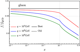
Figure 1: Gluon PDFs in the full unbroken SM, divided by their values assuming pure QCD evolution only. The thin gray lines show where the scales on the x- and/or y-axes switch between linear and logarithmic.

We begin by showing resulting PDFs of strongly interacting particles. Figures 1,  2 and 3 show the evolution of the gluon, and well as left- and right-handed quark PDFs, normalized to their values assuming pure QCD evolution. In each plot we show the results at three different scales, namely $q=10^{4}$, $10^{6}$ and $10^{8}$ GeV. The values of $10^{6}$ and $10^{8}$ GeV are of course far away from energy scales one can reach at any collider in the near or distant future. However, showing the results at such unattainable values helps to illustrate their approach to asymptotic behavior.

The improvements in this paper affect the gluon PDF at a level too small to be noticeable in Figure 1. This is expected because the gluon is overwhelmingly dominated by QCD evolution, and is only affected by electroweak corrections through the back-reaction from quarks.

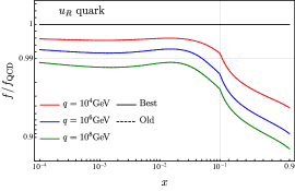
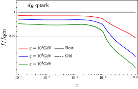
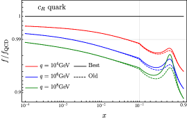
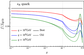
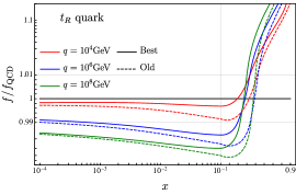
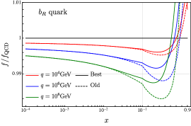
Figure 2: Right-handed quark PDFs in the full unbroken SM, divided by their values assuming pure QCD evolution only. The thin gray lines show where the scales on the x- and/or y-axes switch between linear and logarithmic.

The right-handed quark PDFs have no double-logarithmic component and mainly evolve to slightly lower values than pure QCD, due to energy loss through the additional splitting $q_{R}\to q_{R}B$. The improvements of this paper affect the PDFs only at high $x$ and are much more pronounced for the heavy quarks. This is because heavy quarks are mainly produced perturbatively in QCD, such that the relative electroweak effect is overall larger.

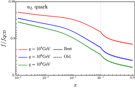
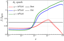
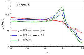
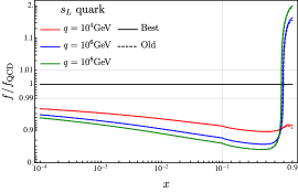
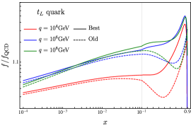
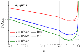
Figure 3: Left-handed quark PDFs in the full unbroken SM, divided by their values assuming pure QCD evolution only. The thin gray lines show where the scales on the x- and/or y-axes switch between linear and logarithmic.

For left-handed quarks, at low $x$, the effects of the improvements of this paper are very small. As discussed in [1], the light quarks (and antiquarks, not shown) evolve to lower values compared to pure QCD at small $x$, due to an overall loss of energy to the electroweak gauge bosons. At large $x$, the effects are more noticeable, and in particular for the heavy quarks lead to ${\cal O}(1)$ relative changes, although the absolute values of the PDFs there are very small. The qualitative features are unchanged, in particular the up and down quarks (top row) exhibit different behaviors, with the left-handed up PDF evolving more rapidly to lower values compared to pure QCD, while the down quark eventually evolves to higher values, as the isovector contribution to their PDFs dies away double-logarithmically.

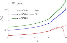
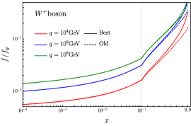
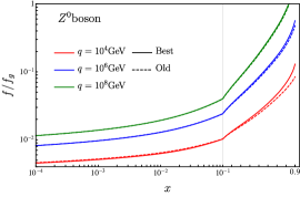
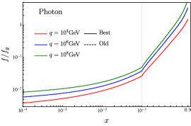
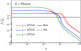
Figure 4: Unpolarized transverse electroweak boson PDFs normalized by the gluon PDF. The thin gray lines show where the scales on the x- and/or y-axes switch between linear and logarithmic.

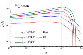
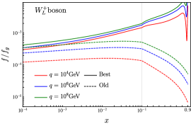
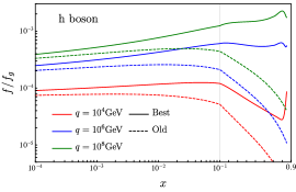
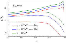
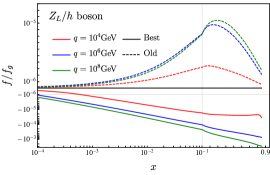
Figure 5: Longitudinal gauge and Higgs boson PDFs normalized by the gluon PDF. The $Z_{L}/h$ PDF is purely imaginary and we show the result divided by $i$. The thin gray line shows where the scales on the x- and/or y-axes switch between linear and logarithmic.

Next, we study the effect on vector boson PDFs. Recall that in [1, 2] the initial values for the heavy gauge bosons at the matching scale $q_{0}$ were zero and their entire effect was generated dynamically through the DGLAP evolution above that scale. In contrast, in this work we use the results of [5] to determine their initial values. These input values are ${\cal O}(\alpha)$ and thus of subleading logarithmic order. At relatively low values of $q$ we therefore expect large effects, while at large $q$ values the logarithmic corrections should dominate, such that the effect of the input decreases. This can be seen clearly in Fig. 4, where we show the ratio of the PDFs relative to the gluon. Since we did not change the initial condition of the photon, its PDF is not affected. For the heavy vector boson PDFs the effect is more pronounced at low values of $q$ and is barely noticeable at the largest value of $q$ shown.

For the longitudinally polarized gauge bosons, the Higgs boson and the mixed PDF between the Higgs and the $Z_{L}$, the effect of the improvements is considerable larger, and at large $x$ changes the PDFs by more than an order of magnitude. This is because their contributions from the dynamical evolution are much smaller, arising only to second order in the electroweak gauge coupling, and through Yukawa couplings to the top quark. The initial values, on the other hand are of the same order as for the transverse vector bosons, namely ${\cal O}(\alpha)$. This can be traced back to the fact that the equivalence theorem, which underlies the DGLAP evolution in the unbroken SM, is badly broken at scales of order of the electroweak scale, manifesting itself through power corrections that are large at threshold (see also [15]). By using the perturbative result as the initial value to the DGLAP evolution, one combines these large threshold corrections with the large logarithmic terms that dominate far above the threshold.

To illustrate the uncertainties associated with subleading terms, we show in Tables 2 and 3 the dependence of some integrated PDFs (momentum fractions) on the infrared cutoff $m_{V}$ and matching scale $q_{0}$. The electroweak PDFs are much less sensitive to these parameters than was the case in Ref. [1], due to the electroweak input at the matching scale. The exception is the Higgs boson, which is still generated dynamically starting from zero at the matching scale.

$m_{V}$/GeV	$q_{0}$/GeV	$u_{L}$	$t_{L}$	$W_{T}^{+}$	$W_{T}^{-}$	$e_{L}^{-}$	$\nu_{e}$	$h$	$Z_{L}^{0}$
100	100	8.51	0.43	0.46	0.34	0.0021	0.0014	0.0044	0.0232
50	100	8.42	0.44	0.46	0.34	0.0020	0.0014	0.0053	0.0233
50	200	8.48	0.44	0.45	0.33	0.0020	0.0013	0.0051	0.0230
100	200	8.57	0.43	0.45	0.32	0.0020	0.0013	0.0043	0.0230
200	200	8.64	0.42	0.45	0.32	0.0020	0.0013	0.0037	0.0231

Table 2: Momentum fractions (%) carried by various parton species at scale $q=10$ TeV.

$m_{V}$/GeV	$q_{0}$/GeV	$u_{L}$	$t_{L}$	$W_{T}^{+}$	$W_{T}^{-}$	$e_{L}^{-}$	$\nu_{e}$	$h$	$Z_{L}^{0}$
100	100	7.52	0.60	0.64	0.50	0.0034	0.0029	0.0107	0.0251
50	100	7.41	0.62	0.64	0.51	0.0034	0.0029	0.0118	0.0251
50	200	7.46	0.62	0.63	0.50	0.0033	0.0028	0.0116	0.0249
100	200	7.57	0.60	0.63	0.50	0.0033	0.0028	0.0105	0.0250
200	200	7.67	0.59	0.63	0.49	0.0034	0.0027	0.0095	0.0250

Table 3: Momentum fractions (%) carried by various parton species at scale $q=100$ TeV.

Finally, we show the size of the vector boson polarization generated by the electroweak evolution in Fig. 6. As already mentioned, polarized vector bosons were not included in our previous results. We can see that for the massive electroweak gauge bosons the polarization is ${\cal O}(1)$, especially at large $x$, and negative owing to the dominance of emission from left-handed fermions. For the photon, and even more so the gluon, the polarization is much smaller.

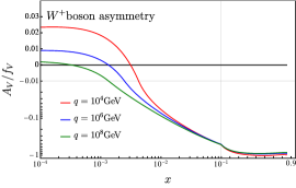
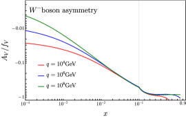
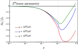
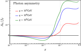
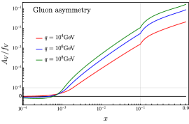
Figure 6: Polarization of gauge bosons normalized to their unpolarized PDFs. The thin gray line shows where the scales on the x- and/or y-axes switch between linear and logarithmic.

In [2] we presented results of the expansion of all PDFs, defining

$$\left[f_{i}^{\rm SM}(x,q)\right]_{\alpha}=f_{i}^{\rm noEW}(x,q)+g_{i}(x,q)\,,$$ (133)

where

$$f_{i}^{\rm noEW}(x,q)=\left\{\begin{array}[]{l}\mbox{QCD+QED evolution for $q<q_{V}$}\,,\\ \mbox{QCD evolution for $q>q_{V}$}\,.\end{array}\right.$$ (136)

and $\left[f_{i}^{\rm SM}(x,q)\right]_{\alpha}$ only includes the linear terms in $\alpha_{I\neq 3}$. These results were used to match the resummed calculation to fixed-order results, and to understand the importance of the resummation and higher-order corrections that are very difficult to obtain in a fixed-order calculation. We have repeated the calculation of the first-order expansion of all PDFs, including all improvements discussed in this paper. While the numerical results change slightly, qualitatively all conclusions made in the previous paper remain unchanged. For this reason, we do not repeat the analysis here. We will, however, study the perturbative convergence of the parton luminosities, discussed next.

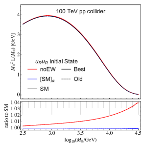
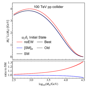
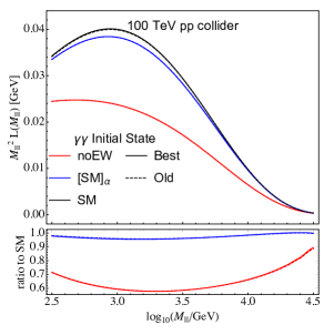
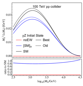
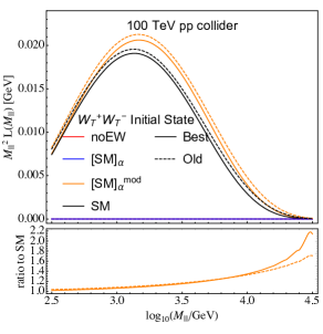
Figure 7: Plots showing luminosities for various choices of initial states. We show in black the luminosity computed using the full SM, in red the result without any EW effects, in blue the first order expansion and for $V_{T}V_{T}$ initial states in orange the luminosity when both first order expansions are multiplied together.

As a final result, we combine the obtained PDFs into parton luminosities at a future 100 TeV $pp$ collider. In Fig. 7 we show the results for a few selected parton luminosities

$${\cal L}^{\rm SM}_{AB}(M_{\ell\ell})=\int\!{\rm d}x_{A}\,{\rm d}x_{B}\,{\cal L}^{\rm SM}_{AB}\left(x_{A},x_{B};M_{\ell\ell}\right)\,\delta\left(M_{\ell\ell}-\sqrt{x_{1}x_{2}S}\right)\,,$$ (137)

with

$${\cal L}^{\rm SM}_{AB}(x_{A},x_{B};Q) =f_{A}^{\rm SM}(x_{A},Q)\,f_{B}^{\rm SM}(x_{B},Q)\,,$$ (138)

for $pp$ collisions at $\sqrt{S}=100$ TeV, rescaled by the square of the invariant mass $M_{\ell\ell}$ to overcome the steeply falling nature of the functions.

For the transverse vector boson luminosities, one needs to consider the positive and negative helicity PDFs of the bosons, such that there are in general four different luminosities for each flavor combination. For the production of fermions (after integrating over the rapidity of the produced fermions), the relevant luminosity is the sum of $V_{+}V_{-}$ and $V_{-}V_{+}$, which is related to the difference of the unpolarized and polarized luminosities

$${\cal L}_{VV}-{\cal L}_{A_{V}A_{V}}=2\left({\cal L}_{V_{+}V_{-}}+{\cal L}_{V_{-}V_{+}}\right).$$ (139)

For this reason, we show this difference, but one has to remember that in general three more luminosities are required.

For each figure, we show in black ${\cal L}^{\rm SM}$ (see Eq. (137)). In red we show ${\cal L}^{\rm noEW}$, computed using PDFs that were evolved using only QCD and QED interactions, as specified in Eq. (136). In blue we show the $\left[{\cal L}^{\rm SM}\right]_{\alpha}$, given by

$$\left[{\cal L}^{\rm SM}_{AB}(x_{A},x_{B};Q)\right]_{\alpha} =f_{A}^{\rm noEW}(x_{A},Q)\,f_{B}^{\rm noEW}(x_{B},Q)+f_{A}^{\rm noEW}(x_{A},Q)\,g_{B}(x_{B},Q)$$

$$\quad+g_{A}(x_{A},Q)\,f_{B}^{\rm noEW}(x_{B},Q)\,,$$ (140)

and for VV initial states in orange $\left[{\cal L}^{\rm SM}\right]_{\alpha}^{\rm mod}$, given by

$$\left[{\cal L}^{\rm SM}_{AB}(x_{A},x_{B};Q)\right]_{\alpha}^{\rm mod} =f_{A}^{\rm noEW}(x_{A},Q)\,f_{B}^{\rm noEW}(x_{B},Q)+f_{A}^{\rm noEW}(x_{A},Q)\,g_{B}(x_{B},Q)$$ (141)

$$\quad+g_{A}(x_{A},Q)\,f_{B}^{\rm noEW}(x_{B},Q)+g_{A}(x_{A},Q)\,g_{B}(x_{B},Q)\delta_{AB,V_{T}V_{T}}\,,$$

which coincides with $\left[{\cal L}^{\rm SM}_{AB}\right]_{\alpha}$ for all channels except $V_{T}V_{T}$.

As for the PDFs, we show in solid lines the results including all effects discussed in this paper, and in dashed lines the results of [2] that does not include these effects. For the $q\bar{q}$ and $\gamma\gamma$ luminosities the effects are so small that two lines are practically indistinguishable. For luminosities involving heavy vector boson PDFs, the effects are larger, as can be expected from the results discussed for those PDFs above. However, qualitatively, all conclusions of [2], in particular about the importance of resummation, are unchanged.

5 Conclusions

We have updated the results of Refs. [1, 2] on parton distribution functions in the full SM by including three effects not considered in that earlier work. The first is the inclusion of gauge boson polarization, the second is to use non-zero input electroweak boson PDFs at the electroweak scale and the final effect is the improvement of the collinear evolution to full next-to-leading-order accuracy.

Gauge boson polarizations arise because left- and right-handed fermions, which evolve differently in the full SM due to their different interactions with the SU(2) and U(1) gauge groups, couple differently to left-and right-handed polarized transverse vector bosons. This effect was first discussed in [4], where it was mentioned that it induces a polarization asymmetry in all transversely polarized gauge bosons. The implementation presented in this work shows that PDFs for the polarized $W_{T}$ and $Z_{T}$ bosons can be as large as their unpolarized PDFs, in particular at large $x$.

In [1, 2] the initial conditions for the SM evolution were determined by treating the PDFs of quarks, gluons and the photon as non-zero at scale 10 GeV and then evolving them to scale $q_{0}\sim 100$ GeV using QCD and QED interactions. This meant that the PDFs for neutrinos, $W$ and $Z$ and Higgs bosons as well as the top quark were zero at $q_{0}$ and therefore only generated dynamically through the SM evolution. In this work, we take the results of [5] to obtain input values for the $W$ and $Z$ bosons (both longitudinal and transverse) at $q_{0}$. This therefore combines the resummation of the large logarithmic terms generated by the evolution with the threshold effects obtained from the fixed order results at $q_{0}$. As shown, this changes the results for electroweak vector bosons at low values of $q$, but these effects become subdominant at large values of $q$.

The final effect is the improvement of the collinear evolution to full next-to-leading-order accuracy. This was already discussed for fragmentation functions in [3], and can be implemented through a proper definition of the running coupling constant. Such higher logarithmic resummation becomes most important at scales for which $\alpha L\sim 1$, which requires extremely large values of $q\sim 10^{15}$ GeV. Thus, one expects that the higher logarithmic effects give rise to only small effects at phenomenologically relevant scales, which is confirmed by our implementation.

References

[1]
C. W. Bauer, N. Ferland and B. R. Webber, Standard Model Parton
Distributions at Very High Energies,
JHEP08 (2017)
036, [1703.08562].
[2]
C. W. Bauer, N. Ferland and B. R. Webber, Combining initial-state
resummation with fixed-order calculations of electroweak corrections,
JHEP04 (2018)
125, [1712.07147].
[3]
C. W. Bauer, D. Provasoli and B. R. Webber, Standard Model Fragmentation
Functions at Very High Energies,
1806.10157.
[4]
A. V. Manohar and W. J. Waalewijn, Electroweak Logarithms in Inclusive
Cross Sections, 1802.08687.
[5]
B. Fornal, A. V. Manohar and W. J. Waalewijn, Electroweak Gauge Boson
Parton Distribution Functions, 1803.06347.
[6]
A. Manohar, P. Nason, G. P. Salam and G. Zanderighi, How bright is the
proton? A precise determination of the photon parton distribution function,
Phys. Rev.
Lett.117 (2016) 242002, [1607.04266].
[7]
A. V. Manohar, P. Nason, G. P. Salam and G. Zanderighi, The Photon
Content of the Proton,
JHEP12 (2017)
046, [1708.01256].
[9]
Y. L. Dokshitzer, D. Diakonov and S. I. Troian, Hard Processes in
Quantum Chromodynamics,
Phys. Rept.58 (1980) 269–395.
[10]
D. Amati, A. Bassetto, M. Ciafaloni, G. Marchesini and G. Veneziano, A
Treatment of Hard Processes Sensitive to the Infrared Structure of QCD,
Nucl. Phys.B173 (1980) 429–455.
[11]
S. Catani, B. R. Webber and G. Marchesini, QCD coherent branching and
semiinclusive processes at large x,
Nucl. Phys.B349 (1991) 635–654.
[12]
J.-y. Chiu, F. Golf, R. Kelley and A. V. Manohar, Electroweak
Corrections in High Energy Processes using Effective Field Theory,
Phys. Rev.D77 (2008) 053004, [0712.0396].
[13]
C. Schmidt, J. Pumplin, D. Stump and C. P. Yuan, CT14QED parton
distribution functions from isolated photon production in deep inelastic
scattering, Phys.
Rev.D93 (2016) 114015, [1509.02905].