Multi-pulse fitting of Transition Edge Sensor signals from a near-infrared continuous-wave source

Abstract

Transition-edge sensors (TES) are photon-number resolving calorimetric spectrometers with near unit efficiency. Their recovery time, which is on the order of microseconds, limits the number resolving ability and timing accuracy in high photon-flux conditions. This is usually addressed by pulsing the light source or discarding overlapping signals, thereby limiting its applicability. We present an approach to assign detection times to overlapping detection events in the regime of low signal-to-noise ratio, as in the case of TES detection of near-infrared radiation. We use a two-level discriminator, inherently robust against noise, to coarsely locate pulses in time, and timestamp individual photoevents by fitting to a heuristic model. As an example, we measure the second-order time correlation of a coherent source in a single spatial mode using a single TES detector.

Contribution of NIST, an agency of the U.S. government, not subject to copyright.

I Introduction

Transition-edge sensors are wideband photon-number resolving light detectors that can be optimized for high quantum efficiency ($>98\%$) and to work in different regions of the electromagnetic spectrum, from soft X-rays to telecom wavelengths Lita et al. (2010a); Fukuda et al. (2011). Their high single photon detection efficiency in the optical band was instrumental in one of the recent loophole-free experimental violations of Bell’s inequality Giustina et al. (2015). Absorption of a single photon by the TES generates an electric pulse response with a fast (tens of nanoseconds) rising edge, and a relaxation with a time constant of a few microseconds Lamas-Linares, Antía et al. (2013). Photodetection events with time separation shorter than the pulse duration overlap and cannot be reliably identified by threshold crossing. To avoid this problem, TES are often used with pulsed light sources with a repetition rate lower than few tens of kilohertz Levine et al. (2012). This may exclude the use of TES with superb detection efficiencies from some applications. Therefore, in this work we investigate the time discrimination for overlapping signal pulses using a continuous-wave (CW) light source.

Similar problems are common in high-energy physics Marrone et al. (2006); Belli et al. (2008); Vencelj et al. (2009); Tambave et al. (2012); Fowler et al. (2015). Fowler et al. Fowler et al. (2015) improved time discrimination by considering the time derivative of the signal to locate the steep rising edge of individual photodetection events. In cases with high signal-to-noise ratio, such as in the detection of high-energy photons  $\gamma$ and X-rays (SNR $\approx$260, estimated from Ref. Fowler et al., 2015), this approach is effective also when signals overlap. However, for near-infrared (NIR) photodetection with a TES, it is necessary to filter high frequency noise components to improve the signal-to-noise ratio (SNR $\approx$2.4, estimated from Ref. Lamas-Linares, Antía et al., 2013) at the expense of a reduced timing accuracy.

We approach the problem by separating it into two distinct phases: an initial event identification, followed by a more accurate timing discrimination. We identify photodetection events using a two-level discriminator. Its resilience to noise allows us to coarsely locate both isolated and overlapping pulses with a moderate use of filtering, thus retaining some of the high frequency components of the signal, useful to improve the time accuracy of subsequent operations. For monochromatic sources, every detection event has the same energy. We can then estimate the number of photons for every detection region from the total pulse area, identifying the cases of overlapping events. From the number of photons, we calculate a heuristic model function and fit it to the signal to recover the detection-times.

II Electronics and photon detection pulse

Figure 1: Schematic of the TES biasing and readout electronics. The TES is voltage-biased by a constant current source $I_{\text{TES}}$ through shunt resistor $R_{\text{shunt}}\ll R_{\text{TES}}$. The SQUID array amplifier picks up changes in TES resistance from $L_{\text{in}}$. The signal is further amplified outside of the cryostat. Signal feedback via $R_{\text{fb}}$ and coil $L_{\text{fb}}$ linearizes the SQUID response.

Our tungsten-based TES Lita, Miller, and Nam (2008) is kept at a temperature of 75 mK using an adiabatic demagnetization refrigerator cryostat, and is voltage biased within its superconducting-to-normal transition in a negative electro-thermal feedback Irwin (1995). The detection signal is inductively picked up and amplified by a SQUID series array, followed by further signal conditioning at room temperature with an overall amplification bandwidth of $\approx$6 MHz. A schematic of the TES biasing and readout electronics is shown in figure 1. We operate the SQUID in a flux-locked loop Drung et al. (2007) to minimize low frequency components of the noise. To characterize the TES response, we use a laser diode centered at 810 nm as a light source, operated in CW mode. We control the average photon flux with a variable attenuator, then launch the light into a fiber (type SMF28e dis ) that directs it to the sensitive surface of the TES.

We record 10 $\mu$s long traces with a sampling rate of $5\times 10^{8}$ s^-1 and a 12 bit voltage resolution. For light at 810 nm, the signal generated by discrete absorption processes for each photon after the amplifier chain exhibits a rise time for a single photon pulse of about 100 ns, and an overall pulse duration of about $2\,\mu$s.

We collected a total of $4\times 10^{5}$ traces with the TES continuously illuminated by an attenuated laser diode. Despite the flux-locked loop, we observe a residual voltage offset variation from trace to trace. Therefore, for every recorded pulse trace $v_{\text{rec}}(t)$, we remove the residual baseline,

$$v(t)=v_{\text{rec}}(t)-V_{M}\,,$$ (1)

where $V_{M}$ is the most frequently occurring value of the discretized signal $v_{\text{rec}}(t)$ over the sampling interval.

III Pulse Identification

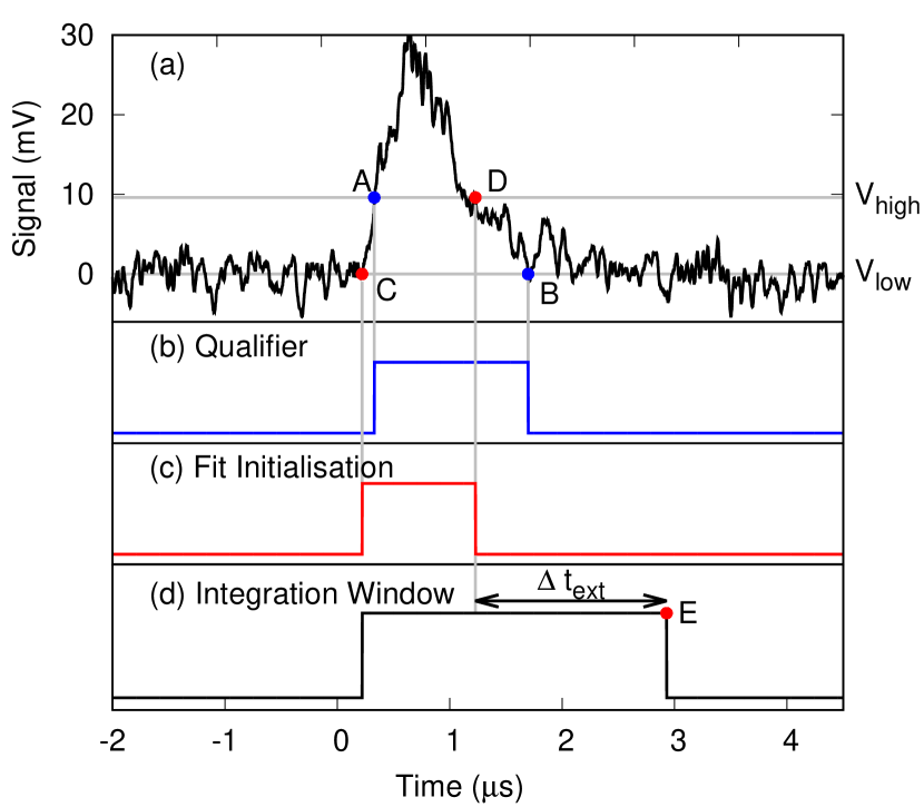
Figure 2: (a) Typical TES response with overlapping pulses. The horizontal lines show the high and low threshold settings of the Schmitt trigger mechanism. (b) Qualifying interval AB identified by the Schmitt trigger. (c) The interval CD includes the rising edges of the overlapping pulses, and is used to initialize a least-square fit. (d) The wider interval CE that includes the rising edge and decaying tail is used to estimate the number of photons associated with the event. We empirically found a reasonable energy resolution with Point E obtained by extending interval CD by $\Delta t_{ext}=1700$ ns.

In a first step, we identify the presence of an absorption process from one or more photons in a trace, and distinguish it from background noise. This is done by a traditional Schmitt trigger mechanism Schmitt (1938), implemented via discriminators at two levels: a qualifier flag is raised when the signal passes threshold $V_{\text{high}}$ (figure 2(a), point A) and lowered by the first subsequent crossing of threshold $V_{\text{low}}$ (point B).

In order to minimize the number of false events, we estimate $V_{\text{high}}$ using a histogram of maximum pulse heights for $4\times 10^{4}$ traces, shown in figure 3. The distribution has two distinct peaks, with one around 5 mV corresponding to traces without any detection event ($n=0$), and another one starting from 9.5 mV onwards corresponding to traces with at least one detection event ($n>0$). We choose $V_{\text{high}}$ to the minimum between the two peaks (9.5 mV), and $V_{\text{low}}$ to 0 mV.

An expected timing accuracy for single photon events that can be extracted from the TES response would be given by the RMS noise (about 1.75 mV), and the steepest slope of the response (0.11(9) mV/ns, estimated from an average of 10%-90% transitions of an ensemble of pulses) to be about 16 ns. However, a simple threshold detection of the leading edge does not work if pulses start to overlap.

More precise timing information of a photodetection event is obtained from a least square fit to the signal using a displaced standard pulse. To efficiently initialize this fit, we do not directly use the qualifier window AB for two reasons: first, it contains only a fraction of the leading edge belonging to the earlier pulse that contains most of the timing information, and second, it includes a large portion of the decaying tail unassociated with the onset of photodetection. The time window CD derived from the same discriminator levels ensures the inclusion of the first leading edge, and is also shorter.

Similarly, we derive an integration time window from the qualifier window to determine the pulse integral, from which we extract the photon number of a quasi-monochromatic light source. As a starting point, we choose point C for the integration to capture the rising slope of a pulse, and extend the time D by a fixed amount $\Delta t_{ext}$ to point E to capture the tail of the response signal (figure 2(d)). We found that it is more reliable to extend point D by a fixed time to capture the tail of the signal rather than to reference the end of the integration window to point B. This is because the signal-to-noise ratio around B is low, leading to a large variation of integration times. We empirically find that $\Delta t_{ext}=1700$ ns gives a good signal-to-noise ratio of the pulse integral.

Figure 3: Histogram of maximum pulse heights for $4\times 10^{5}$ traces. The two distributions correspond to traces with ($n>0$) and without ($n=0$) photodetection events. We use the minimum between the two distributions to set the threshold $V_{\text{high}}$ of the discriminator.

IV Photon Number Discrimination

To determine the number of photons in each trace, we assume that the detection and subsequent amplification have a linear response, so that the integral of each signal is proportional to the absorbed energy Cabrera et al. (2000), resulting in a discrete distribution of the areas of the signals. This distribution is spread out by noise, and we have to use an algorithm to extract the photon number in presence of this noise.

For this, we first compute the pulse area $a=\int_{t_{C}}^{t_{E}}|v(t)|$ for every qualified trace within region CE. Figure 4 shows a histogram of pulse areas from the qualified traces out of all the $4\times 10^{5}$ acquired. The distribution shows three resolved peaks that suggest having been caused by $n=1,2,3$ photons being absorbed by the TES.

One can fit the histogram in figure 4 to a sum of three normalized Gaussian peaks $g_{n}(a;a_{n},\sigma_{n})$ ,

$$H(a)=\sum_{n=1}^{3}h_{n}\,g_{n}(a|a_{n},\sigma_{n})\,,$$ (2)

where each Gaussian peak is characterized by an average area $a_{n}$ and width $\sigma_{n}$. The ratio $a_{2}/a_{1}=1.95$ indicates that the TES response to photon energies of 1 and 2 photons is approximately linear.

We identify thresholds $a_{n-1,n}$ as the values that minimize the overlap between distributions $g_{n-1}(a|a_{n-1},\sigma_{n-1})$ and $g_{n}(a|a_{n},\sigma_{n})$. With this, we assign a number of detected photons $n$ by comparing the area of every trace to thresholds $a_{n-1,n}$ and $a_{n,n+1}$.

The continuous nature of the light source with a fixed power level makes it difficult to assign a number of photons per qualified signal, as the integration window varies from pulse to pulse, and detection events may occur at random times in the respective integration windows. Heuristically, however, one could even replace the individual event numbers $h_{n}$ in Eq. 2 by a Poisson distribution,

$$h_{n}=Np(n|\bar{n})\,,$$ (3)

where $\bar{n}$ is an average photon number, $p(n|\bar{n})$ the Poisson coefficient, and $N$ is the total number of traces. For the data shown in figure 4, this would lead to an average photon number of $\bar{n}\approx 0.3$ per integration time interval.

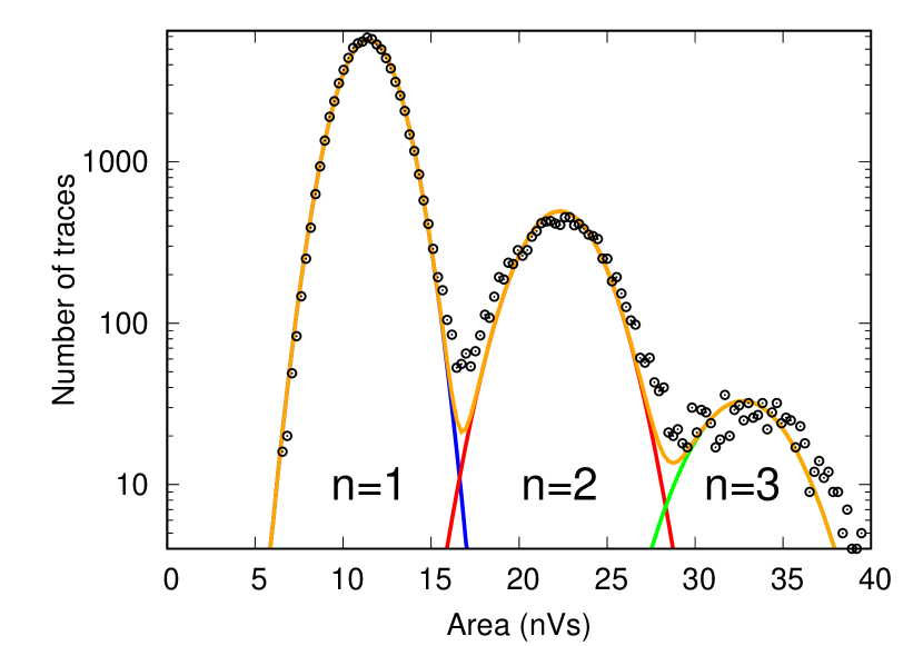
Figure 4: Distribution of pulse areas $H(a)$. For every trace that triggers the two-levels discriminator, the area is calculated within the region CE. The continuous lines are Gaussian fits for the $n=1$ (blue), $n=2$ (red), and $n=3$ (green) area distributions, and their sum (orange).

V Determining the detection-times of overlapping pulses

The difficulty of assigning a photon number to light detected from a CW source can be resolved if one treats the first detection process of light following the paradigm of wideband photodetectors in quantum optics Glauber (1963). As TES are sensitive over a relatively wide optical bandwidth, the corresponding time scale of the absorption process is much shorter than the few microseconds of the TES thermal recovery Gerrits et al. (2016). Then, the signal would correspond to a superposition of responses to individual absorption processes, which may happen at times closer than the characteristic pulse time.

To recover absorption times of individual absorption events in a trace of $N$ overlapping pulses, where $N$ is determined with the pulse area method outlined in the previous section, we fit the TES response signal $v(t)$ to a heuristic model $v_{N}(t)$ of a linear combination of single-photon responses $v_{1}(t)$,

$$v_{N}(t|\{t_{i},A_{i}\}))=\sum_{i=1}^{N}\,A_{i}\,v_{1}(t-t_{i})\,,$$ (4)

where $A_{i}$ is the amplitude and $t_{i}$ the detection time of the $i$-th pulse. While the TES response to multi-photon events is not strictly linear, this model will give a reasonably good estimation of the timing for single photon absorption events.

V.1 Single photon pulse model

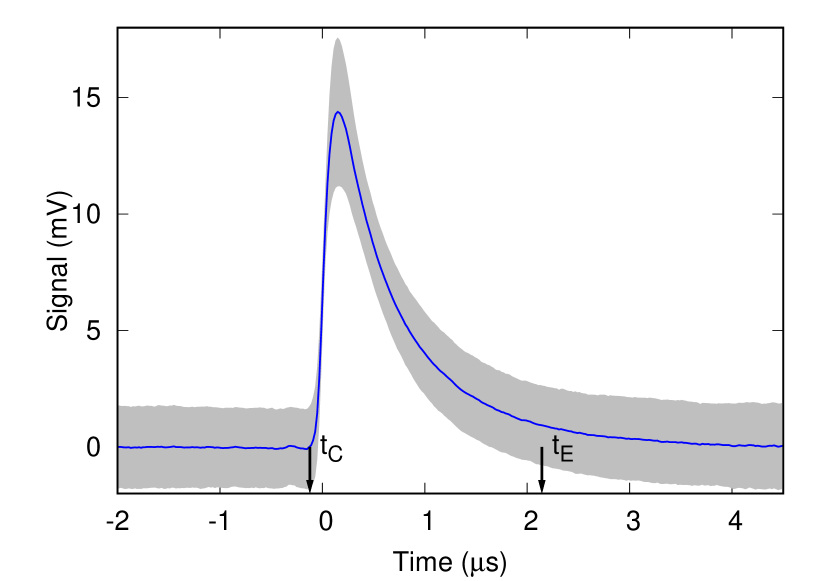
Figure 5: Solid line: average response of the TES and amplification to a single absorption. We use a Schmitt trigger to identify the region between $t_{C}$ and $t_{E}$. Grey region: one standard deviation in the observed ensemble of $n=1$ traces.

We obtain a model for the single photon response $v_{1}(t)$ of the TES and its signal amplification chain for the fit in Eq. 4 by selecting $N_{1}=10^{4}$ single photon traces from the measurement shown in figure 4, and averaging over them. The averaging process eliminates the noise from individual traces, and retains the detector response.

Signal photon events can happen at any time within the sampling window. It is necessary to align these detection events to average the traces. We assign a detection time to the $i$-th trace $v_{1}^{(i)}(t)$ by recording the time $t_{i}$ corresponding to the maximum of $dv_{1}^{(i)}(t)/dt$. We use a Savitzky-Golay filter (SGF) to reduce the high frequency components Savitzky and Golay (1964); the SGF replaces every point with the result of a linear fit to the subset of adjacent 41 points.

We also reject clear outlier traces by limiting the search for $t_{i}$ to the time interval CD. The remaining $N_{1}$ traces are then averaged by synchronizing them according to their respective $t_{i}$ and to obtain the single-photon response $v_{1}(t)$,

$$v_{1}(t)=\frac{1}{N_{1}}\sum_{i=1}^{N_{1}}v_{1}^{(i)}(t+t_{i})\,.$$ (5)

The result is shown in figure 5, together with a noise interval derived from the standard deviation of $N_{1}$ single photon traces. The model demonstrates an average rise time of 116 ns from 10% to 90% of its maximum height. The relaxation time (1/$e$) of 635 ns corresponds to detector thermalization Lita et al. (2010b).

V.2 Time-tagging via least-square fitting

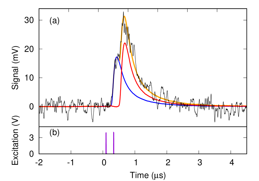
Figure 6: (a) Fit of a two-photon signal with the heuristic function described in the main text. Black line: measured TES response after removing the vertical offset. Orange line: fit to Eq. (4), with two single photon components separated in time (blue and red line). (b) Electrical pulse pair separated by 239 ns sent to the LD illuminating the TES.

For every qualified trace, we assign a number of photons $N$ according to the calculated area, and fit it using Eq. (4). The fit has $2\,N$ free parameters: detection times $t_{i}$ and amplitudes $A_{i}$, with $i=1\dots N$. We bound $t_{i}$ to the range CD (figure 2(c)), and restrict the sum of $A_{i}$ to be consistent with the thresholds obtained from the area distribution

$$\frac{a_{N-1,N}}{\int_{t_{C}}^{t_{E}}|v_{1}(\tau)|\,d\tau}\leq\sum_{i=1}^{N}A_{i}\leq\frac{a_{N,N+1}}{\int_{t_{C}}^{t_{E}}|v_{1}(\tau)|\,d\tau}\,.$$ (6)

The accuracy of the fit depends on the choice of minimization algorithm. We used Powell’s derivative-free method Powell (1964) because the presence of noise tends to corrupt gradient estimation P. Plagianakos and Vrahatis (2002).

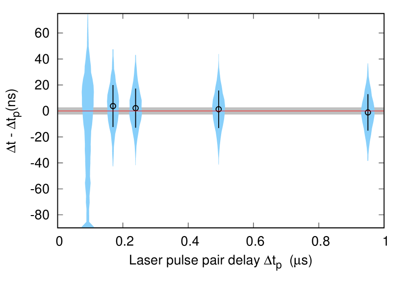
Figure 7: Difference between the detection-time separation estimated with the fitting technique ($\Delta t$) and the delay of laser pulse pairs ($\Delta t_{p}$) for five different delays: 92 ns, 170 ns, 239 ns, 493 ns, and 950 ns. Blue regions: distribution of $\Delta t-\Delta t_{p}$. Grey region: expected range of separation for 90% of single photon detections for 4 ns long laser pulse pairs. Black circles: mean of the distributions with error bars corresponding to one standard deviation.

To verify the accuracy of the fitting algorithm for $N=2$, we expose the TES to pairs of short (4 ns) laser pulses with a controlled delay $\Delta t_{p}$. The 100 kHz repetition rate is low enough to isolate the TES response between consecutive laser pulse pairs. Selecting only the traces with two photons, we have two possible cases: (i) a two-photon event generated within one of the 4 ns pulses or (ii) one photon in each pulse. We compared the TES response for five different delays $\Delta t_{p}$: 92 ns, 170 ns, 239 ns, 493 ns, and 950 ns. Figure 6 shows an example of a measured trace where the fitting algorithm was able to distinguish between separate photodetection events at $\Delta t_{p}=239$ ns even though it appears to be a single event because of the detector noise. For each delay we collected $\approx 3.5\times 10^{5}$ traces, and for each trace we estimate the photodetection times using the least-square method. In figure 7 we summarize the distribution of time differences $\Delta t=|t_{2}-t_{1}|$ for each delay.

Except for the shortest pulse separation, the time differences have Gaussian distributions with standard deviations of about 16 ns. This matches the time accuracy expected from the simple noise/slope estimation for the leading edge of the single photon pulse, despite the overlapping pulses. The average separation between the center of the distribution and the expected result, $\Delta t-\Delta t_{p}$, is 2(2) ns. For $\Delta t_{p}=92$ ns, the distribution is clearly skewed toward $0$ ns. This multi-modal distribution indicates that the fit procedure is unable to distinguish two single-photon events generated by the two separated diode pulses from two-photon events generated within the same diode pulse.

VI Detection-Time Separation from coherent source

As another benchmark for the fitting technique presented in here, we extract the normalized second order correlation function $g^{(2)}(\Delta t)$ for detection events recorded with a single TES from a coherent light field. For a light field in a coherent state, this correlation function should be exactly 1 for all time differences $\Delta t$ Glauber (1963).

For this, the TES is exposed to light from a continuously running laser diode, with an average photon number of about 0.3 per integration interval of around 3 $\mu$s. Again, we select only two-photon traces using the methods described in section IV, and fit the traces to the model described by equation 4 with $N=2$.

Figure 8: Normalized second order correlation function $g^{(2)}(\Delta t)$ for events recorded with a single TES from a coherent light field. Error bars indicate one standard deviation assuming Poissonian statistics, the bin size is 25 ns. Solid line: expected correlation for a coherent field.

Each fitted trace leads to two time values $t_{1}$ and $t_{2}$, which we sort into a frequency distribution $G^{(2)}(\Delta t)$ of time differences $\Delta t=t_{2}-t_{1}$. We normalize this distribution with the distribution expected for a Poissonian source, taking into account the finite time of our acquisition windows. We remove single-photon traces mis-identified as two-photon traces by filtering out traces that have a minimum estimated amplitude smaller than one half of a single photon pulse.

The resulting normalized distribution $g^{(2)}(\Delta t)$ is shown in figure 8. For $\Delta t>150$ ns, the correlation function is compatible with the expected value of 1. For shorter time differences, the fit algorithm occasionally locks on the same detection times $t_{1}$ and $t_{2}$, redistributing pair events to $\Delta t=0$, resulting in a calculated correlation then deviates from the expected behavior, including the unphysical value $g^{(2)}(\Delta t=0)>2$. This instability region ($\Delta t<150$ ns) is comparable with the rise time of the average single-photon pulse, and is consistent with the precision indicated in figure 7.

VII Conclusion

We demonstrated a signal processing method based on a Schmitt-trigger based data acquisition and a linear algorithm that can reliably extract both a photon number and photodetection times from the signal provided by an optical Transition Edge Sensor (TES) with an accuracy that is mostly limited by the detector time jitter.

Using this method, we successfully resolved between $n=1,2$ and $3$ photons from a CW NIR source, using the signal integral evaluated in the time interval identified by the discriminator. The time interval includes a greater fraction of the photodetection signal than that considered by a single-threshold discriminator. By considering an optimal fraction of the pulse profile, we obtained pulse integral distributions that sufficiently resolve between photon numbers. We note that the maximum pulse height is unsuitable for photon number discrimination of a CW source since the maximum height depends on the photodetection times when pulses are overlapped. This is evident in figure 3. In contrast, figure 4 shows that $n=1,2$ and $3$ photon events are well resolved using the pulse integral, which does not depend on photodetection times.

This technique provides an alternative to photon counting using edge detection on the differentiated signal Fowler et al. (2015) when signal-to-noise ratio is low.

The discriminated region is then used to initialize a least-squares fit of a signal containing two overlapping pulses to a two-photon model, returning the amplitudes and detection-times of the individual photons.

With the available TES, we can distinguish two photodetection events within about 200 ns using this method. The highest detection rate that can be processed is thus estimated to be about $5\times 10^{6}$ s^-1, compared to about $4\times 10^{5}$ s^-1 if we were to discard overlapping pulses.

Potential applications include the measurement of time-resolved correlation functions using the TES without the need for the spatial multiplexing of several single-photon non-photon-number resolving detectors, provided that the coherence time of the light source is larger than the timing resolution of this technique. The order of the correlation function measured is limited only by the maximum number of photons resolvable by the TES.

References

- Lita et al. (2010a) A. E. Lita, B. Calkins, L. A. Pellouchoud, A. J. Miller, and S. Nam, SPIE Defense, Security, and Sensing 7681, 76810D (2010a).
- Fukuda et al. (2011) D. Fukuda, G. Fujii, T. Numata, K. Amemiya, A. Yoshizawa, H. Tsuchida, H. Fujino, H. Ishii, T. Itatani, S. Inoue, and T. Zama, Opt. Express 19, 870 (2011).
- Giustina et al. (2015) M. Giustina, M. A. M. Versteegh, S. Wengerowsky, J. Handsteiner, A. Hochrainer, K. Phelan, F. Steinlechner, J. Kofler, J.-A. Larsson, C. Abellán, W. Amaya, V. Pruneri, M. W. Mitchell, J. Beyer, T. Gerrits, A. E. Lita, L. K. Shalm, S. W. Nam, T. Scheidl, R. Ursin, B. Wittmann, and A. Zeilinger, Phys. Rev. Lett. 115, 250401 (2015).
- Lamas-Linares, Antía et al. (2013) Lamas-Linares, Antía, B. Calkins, N. A. Tomlin, T. Gerrits, A. E. Lita, J. Beyer, R. P. Mirin, and S. Nam, Appl. Phys. Lett. 102, 231117 (2013).
- Levine et al. (2012) Z. H. Levine, T. Gerrits, A. L. Migdall, D. V. Samarov, B. Calkins, A. E. Lita, and S. W. Nam, J. Opt. Soc. Am. B 29, 2066 (2012).
- Marrone et al. (2006) S. Marrone, E. Berthomieux, F. Becvar, D. Cano-Ott, N. Colonna, C. Domingo-Pardo, F. Gunsing, R. C. Haight, M. Heil, F. Käppeler, M. Krtička, P. Mastinu, A. Mengoni, P. M. Milazzo, J. O’Donnell, R. Plag, P. Schillebeeckx, G. Tagliente, J. L. Tain, R. Terlizzi, and J. L. Ullmann, Nuclear Instruments and Methods in Physics Research, Section A: Accelerators, Spectrometers, Detectors and Associated Equipment 568, 904 (2006).
- Belli et al. (2008) F. Belli, B. Esposito, D. Marocco, M. Riva, Y. Kaschuck, and G. Bonheure, Nuclear Instruments and Methods in Physics Research Section A: Accelerators, Spectrometers, Detectors and Associated Equipment 595, 512 (2008).
- Vencelj et al. (2009) M. Vencelj, K. Bučar, R. Novak, and H. J. Wörtche, Nuclear Instruments and Methods in Physics Research, Section A: Accelerators, Spectrometers, Detectors and Associated Equipment 607, 581 (2009).
- Tambave et al. (2012) G. Tambave, E. Guliyev, M. Kavatsyuk, F. Schreuder, and H. Löhner, IEEE Nuclear Science Symposium Conference Record , 2163 (2012).
- Fowler et al. (2015) J. W. Fowler, B. K. Alpert, W. B. Doriese, D. A. Fischer, C. Jaye, Y. I. Joe, G. C. O’Neil, D. S. Swetz, and J. N. Ullom, ApJS 219, 35 (2015).
- Lita, Miller, and Nam (2008) A. E. Lita, A. J. Miller, and S. W. Nam, Opt. Express 16, 3032 (2008).
- Irwin (1995) K. D. Irwin, Appl. Phys. Lett. 66, 1998 (1995).
- Drung et al. (2007) D. Drung, C. Assmann, J. Beyer, A. Kirste, M. Peters, F. Ruede, and T. Schurig, IEEE Trans. Appl. Supercond. 17, 699 (2007).
- (14) Certain commercial equipment, instruments or materials are identified in this report to foster understanding. Such identification does not imply recommendation or endorsement by the National Institute of Standards and Technology, nor does it imply that the materials or equipment are necessarily the best available for the purpose. .
- Schmitt (1938) O. H. Schmitt, J. Sci. Instrum. 15, 24 (1938).
- Cabrera et al. (2000) B. Cabrera, R. Clarke, A. Miller, S. W. Nam, R. Romani, T. Saab, and B. Young, Physica B: Condensed Matter 280, 509 (2000).
- Glauber (1963) R. J. Glauber, Phys. Rev. 130, 2529 (1963).
- Gerrits et al. (2016) T. Gerrits, A. E. Lita, B. Calkins, and S. W. Nam, in Superconducting Devices in Quantum Optics (Springer International Publishing, Cham, 2016) pp. 31–60.
- Savitzky and Golay (1964) A. Savitzky and M. Golay, Analytical chemistry, 36, 1627 (1964).
- Lita et al. (2010b) A. E. Lita, B. Calkins, L. A. Pellouchoud, A. J. Miller, and S. W. Nam, SPIE Defense, Security, and Sensing 7681, 76810D (2010b).
- Powell (1964) M. J. D. Powell, The Computer Journal 7, 155 (1964).
- P. Plagianakos and Vrahatis (2002) V. P. Plagianakos and M. Vrahatis, Combinatorial and Global Optimization (2002) pp. 283–296.