The Social Cost of Strategic Classification

Abstract.

Consequential decision-making typically incentivizes individuals to behave strategically, tailoring their behavior to the specifics of the decision rule. A long line of work has therefore sought to counteract strategic behavior by designing more conservative decision boundaries in an effort to increase robustness to the effects of strategic covariate shift.

We show that these efforts benefit the institutional decision maker at the expense of the individuals being classified. Introducing a notion of social burden, we prove that any increase in institutional utility necessarily leads to a corresponding increase in social burden. Moreover, we show that the negative externalities of strategic classification can disproportionately harm disadvantaged groups in the population.

Our results highlight that strategy-robustness must be weighed against considerations of social welfare and fairness.

1. Introduction

As machine learning increasingly supports consequential decision making, its vulnerability to manipulation and gaming is of growing concern. When individuals learn to adapt their behavior to the specifics of a statistical decision rule, its original predictive power will deteriorate. This widely observed empirical phenomenon, known as Campbell’s Law or Goodhart’s Law, is often summarized as: “Once a measure becomes a target, it ceases to be a good measure” (Strathern, 1997).

Institutions using machine learning to make high-stakes decisions naturally wish to make their classifiers robust to strategic behavior. A growing line of work has sought algorithms that achieve higher utility for the institution in settings where we anticipate a strategic response from the the classified individuals (Dalvi et al., 2004; Brückner et al., 2012; Hardt et al., 2016a). Broadly speaking, the resulting solution concepts correspond to more conservative decision boundaries that increase robustness to some form of distributional shift.

But there is a flip side to strategic classification. As insitutional utility increases as a result of more cautious decision rules, honest individuals worthy of a positive classification outcome may face a higher bar for success.

The costs incurred by individuals as a consequence of strategic classification are by no means hypothetical, as the example of lending shows. In the United States, credit scores are widely deployed to allocate credit. However, even creditworthy individuals routinely engage in artificial practices intended to improve their credit scores, such as opening up a certain number of credit lines in a certain time period (Citron and Pasquale, 2014).

In this work, we study the tension between accuracy to the institution and impact to the individuals being classified. We first introduce a general measure of the cost of strategic classification, which we call the social burden. Informally, the social burden measures the expected cost that a positive individual needs to incur to be correctly classified correctly.

For a broad class of cost functions, we prove there exists an intrinsic trade-off between institutional accuracy and social burden: any increase in institutional accuracy comes at an increase in social burden. Moreover, we precisely characterize this trade-off and show the commonly considered Stackelberg equilibrium solution achieves maximal institutional accuracy at the expense of maximal social burden.

Equipped with this generic trade-off result, we turn towards a more careful study of how the social burden of strategic classification impacts different subpopulations. We find that the social burden can fall disproportionally on disadvantaged subpopulations, under two different notions by which one group can be disadvantaged relative to another group. Furthermore, we show that as the institution improves its accuracy, it exacerbates the gap between the burden to an advantaged and disadvantaged group. Finally, we illustrate these conditions and their consequences with a case study on FICO data.

1.1. Our Contributions

In this paper, we make the following contributions:

1. We prove a general result demonstrating the trade-off between institutional accuracy and individual utility in the strategic setting. Our theoretical characterization is supplemented with examples illustrating when an institution would prefer to operate along different points in this trade-off curve.

2. We show fairness considerations inevitably arise in the strategic setting. When individuals incur cost as a consequence of making a classifier robust to strategic behavior, we show the costs can disproportionally fall by disadvantaged subpopulations. Furthermore, as the institution increases its robustness, it also increases the disparity between subpopulations.

3. Using FICO credit data as a case-study, we empirically validate our modeling assumptions and illustrate both the general trade-offs and fairness concerns involved with strategic classification in a concrete setting.

Reflecting on our results, we argue that the existing view of strategic classification has been instituition-centric, ignoring the social burden resulting from improved institutional utility. Our framework makes it possible to select context-specific trade-offs between institutional and individual utility, leading to a richer space of solutions.

Another key insight is that discussions of strategy-robustness must go hand in hand with considerations of fairness and the real possibility that robustness-promoting mechanisms can have disparate impact in different segments of the population.

2. Model

Strategic classification.

Throughout this work, we consider the binary classification setting. Each individual has features $x\in\mathcal{X}$ and a label $y\in\mathcal{Y}=\{0,1\}$. The institution publishes a classifier $f:\mathcal{X}\rightarrow\mathcal{Y}$. In the non-strategic setting, the institution maximizes the non-strategic utility, which is simply the classification accuracy of $f$:

$$\mathcal{U}(f)=\mathbb{P}(f(x)=y)\,.$$

In the strategic setting, the individual can modify their features, and the institution aims to preempt the individual’s strategic manipulation. In response to the institution’s classifier $f$, the individual can change her features $x$ to new features $x^{\prime}$. However, modification incurs a cost given by $c:\mathcal{X}\times\mathcal{X}\rightarrow\mathbb{R}_{\geq 0}$. The individual then receives an individual utility $u_{x}(f,x^{\prime})=f(x^{\prime})-c(x,x^{\prime})$, which trades off between the cost of manipulation $c(x,x^{\prime})$ and the benefits of classification $f(x^{\prime})$.

The institution models the individual $x$ as maximizing their utility $u_{x}(f,x^{\prime})$ and acting according to the best-response to the classifier $f$:

$$\Delta(x;f)=\operatorname*{arg\,max}_{x^{\prime}}u_{x}(f,x^{\prime}).$$

When it is clear from context we will drop the dependence on $f$ and write the individual’s best response as $\Delta(x)$. Although $\Delta(x)$ may not have a unique maximizer, it is assumed that the individual $x$ does not adapt her features if she is already accepted by the classifier, i.e. $f(x)=1$, or if there is no maximizer $x^{\prime}$ she can move to such that $f(x^{\prime})=1$. In cases where the individual does adapt, let $x^{\prime}$ be an arbitrary maximizer such that $f(x^{\prime})=1$. In practice, it is unlikely individuals actually play best-response solutions, and we will discuss as appropriate the impact of deviations from best-response play.

Given this model, the institution aims to maximize the strategic utility, which measures accuracy after individual responses:

$$\mathcal{U}_{\Delta}(f)=\mathbb{P}(f(\Delta(x))=y).$$

For example, imagine that the institution is trying to rank pages on a social network. Although the number of likes a page has may be predictive, it is also an easy feature to game. Therefore, models with high strategic utility will assign low weight to this feature, even if it is useful in the static setting. Henceforth, we will refer to the strategic utility as simply the institutional utility.

Social burden.

Focusing purely on maximizing $\mathcal{U}_{\Delta}$, as done in prior work, ignores the cost a classifier imposes on individuals (Brückner and Scheffer, 2011; Hardt et al., 2016b; Dong et al., 2018). To account for these costs, we define the individual burden of a classifier $f$ as the minimum cost an individual needs to incur in order to be classified positively: $b_{f}(x)=\min_{f(x^{\prime})=1}c(x,x^{\prime})$.

For positive individuals with $y=1$, a high individual burden means the individual has to incur great cost to obtain the correct classification. To quantity this cost, we introduce the social burden, defined as the expected individual burden of positive individuals.

Definition 2.0 (Social burden).

The social burden of a classifier $f$ is defined as $\mathcal{B}_{+}(f)=\mathbb{E}\left[b_{f}(x)\mid y=1\right]$.

The social burden measures the expected cost that positive individuals would need to incur to be classified positively, regardless of whether the best response $\Delta(x)$ indicates that they should adapt. One could imagine other ways of measuring the impact on individuals, such as the expected utility of positive individuals, $\mathbb{E}\left[u_{x}(f,\Delta(x))\mid y=1\right]$, or the corresponding measure over all individuals, rather than only positive individuals. Most of our results still hold for these alternative measures, and we relegate discussion about the choice of social burden to Section 7.

Assumptions on cost function.

While there are many possible models for the cost function, we restrict our attention to a natural set of cost functions that we call outcome monotonic. Outcome monotonic costs capture two intuitive properties: (1) Monotonically improving one’s outcome requires monotonically increasing amounts of work, and (2) it is zero cost to worsen one’s outcome. This captures the intuition that, for example, it is harder to pay back loans than it is to go bankrupt.

Definition 2.0 (Outcome likelihood).

The outcome likelihood of an individual $x$ is $\ell(x)=\mathbb{P}(Y=1\mid X=x)$.

We assume that all individuals have a positive outcome likelihood, i.e, $\ell(x)>0$ for all $x$.

Definition 2.0 (Outcome Monotonic Cost).

A cost function $c:\mathcal{X}\times\mathcal{X}\rightarrow\mathbb{R}_{\geq 0}$ is outcome monotonic if for any $x,x^{\prime},x^{*}\in X$ the following properties hold.

• Zero-cost to move to lower outcome likelihoods. $c(x,x^{\prime})>0$ if and only if $\ell(x^{\prime})>\ell(x)$.

• Monotonicity in first argument. $c(x,x^{*})>c(x^{\prime},x^{*})>0$ if and only if $\ell(x^{*})>\ell(x^{\prime})>\ell(x)$.

• Monotonicity in second argument. $c(x,x^{*})>c(x,x^{\prime})>0$ if and only if $\ell(x^{*})>\ell(x^{\prime})>\ell(x)$.

Under these assumptions, we can equivalently express the cost as a cost over outcome likelihoods, $c_{L}:\ell(\mathcal{X})\times\ell(\mathcal{X})\rightarrow\mathbb{R}_{\geq 0}$, defined in the following lemma.

Lemma 2.0.

When the cost function $c(x,x^{\prime})$ is outcome monotonic, then it can be written as a cost function over outcome likelihoods $c_{L}(l,l^{\prime})\coloneqq c(x,x^{\prime})$ where $x,x^{\prime}\in\mathcal{X}$ are any points such that $l=\ell(x)$ and $l^{\prime}=\ell(x^{\prime})$.

Proof.

The monotonicity assumptions imply that if $\ell(x^{*})=\ell(x^{\prime})$, then $c(\cdot,x^{\prime})=c(\cdot,x^{*})$ and $c(x^{\prime},\cdot)=c(x^{*},\cdot)$. Thus, $c_{L}(l,l^{\prime})\coloneqq c(x,x^{\prime})$ is well-defined because any points $x$ and $x^{\prime}$ such that $l=\ell(x)$ and $l^{\prime}=\ell(x^{\prime})$ yield the same value of $c(x,x^{\prime})$. ∎

Throughout the paper, we will make use of the equivalent likelihood cost $c_{L}$ when a proof is more naturally expressed with $c_{L}$, rather than with the underlying cost $c$.

3. Institutional Utility Versus Social Burden

In this section, we characterize the inherent trade-offs between institutional utility and social burden in the strategic setting. In particular, we show any classifier that improves institutional utility over the best classifier in the static setting causes a corresponding increase in social burden.

To prove this result we first show that any classifier can be represented as a threshold classifier that accepts all individuals with outcome likelihood greater than some threshold $\tau\in[0,1]$. Then, we show increasing utility for the institution requires raising this threshold $\tau$, but that this always increases the social burden.

Equipped with this result, we show the (Pareto-optimal) set of classifiers that increase institutional utility in the strategic setting corresponds to an interval $I$. Each threshold $\tau\in I$ represents a particular trade-off between institutional utility and social burden. Strategic classification corresponds to one extremum: the best strategic utility but the worst social burden. The non-strategic utility corresponds to the other: doing nothing to prevent gaming. Neither is likely to be the right trade-off in practical contexts. Real domains will require a careful weighting of these two utilities, leading to a choice somewhere in between. Thus, a main contribution of our work is exposing this interval.

3.1. General Trade-Off

We now proceed to prove the trade-off between institutional utility and social burden. Our first step is to show that in the strategic setting we can restrict attention to classifiers that threshold on the outcome likelihood (assuming the cost is outcome monotonic as in Definition 2.3).

Definition 3.0 (Outcome threshold classifier).

An outcome threshold classifier $f$ is a classifier of the form $f(x)=\mathbb{I}\{\ell(x)\geq\tau\}$ for $\tau\in[0,1]$.

In practice, the institution may not know the outcome likelihood $\ell(x)=\mathbb{P}(Y=1\mid X=x)$. However, as shown in the next lemma, for any classifier that they do use, there is a threshold classifier with equivalent institutional utility and social burden. Thus, we can restrict our theoretical analysis to only consider threshold classifiers.

Lemma 3.0.

For any classifier $f$ there is an outcome threshold classifier $f^{\prime}$ such that $\mathcal{U}_{\Delta}(f)=\mathcal{U}_{\Delta}(f^{\prime})$ and $\mathcal{B}_{+}(f)=\mathcal{B}_{+}(f^{\prime})$.

Proof.

Let $\tau(f)=\min_{x:f(x)=1}\ell(x)$ be the minimum outcome likelihood at which an individual is accepted by the classifier $f$. Then, let $f^{\prime}(x)=\mathbb{I}\{\ell(x)\geq\tau(f)\}$ be the outcome threshold classifier that accepts all individuals above $\tau(f)$. We will show that the institutional utility and social burden of $f$ and $f^{\prime}$ are equal.

Since the cost function is outcome monotonic, it is the same cost to move to any point with the same outcome likelihood. Furthermore, it is higher cost to move to points of higher likelihood, i.e, if $\ell(x^{\prime})>\ell(x^{*})>\ell(x)$, then $c(x,x^{\prime})>c(x,x^{*})>0$. Since individuals game optimally, when an individual changes her features in response to the classifier $f$, she has no incentive to move to a point with likelihood higher than $\tau(f)$ – that would just cost more. Therefore, she will move to any point with likelihood $\tau(f)$ to be accepted by $f$ and will incur the same cost, regardless of which point it is. Thus, we can write the set of individuals accepted by $f$, $\mathcal{A}_{\Delta}(f)$, as

$$\mathcal{A}_{\Delta}(f) =\{x\mid f(\Delta(x))=1\}$$

$$=\{x\mid\exists x^{\prime}:f(x^{\prime})=1,~{}c(x,x^{\prime})\leq 1\}$$

$$=\{x\mid\exists~{}x^{\prime}:\ell(x^{\prime})=\tau(f),~{}c(x,x^{\prime})\leq 1\}\,.$$

Since $\tau(f)=\tau(f^{\prime})$, the individuals accepted by $f$ and $f^{\prime}$ are equal: $\mathcal{A}_{\Delta}(f)=\mathcal{A}_{\Delta}(f^{\prime})$. Therefore, their institutional utilities $\mathcal{U}_{\Delta}(f)$ and $\mathcal{U}_{\Delta}(f^{\prime})$ are equal. We can similarly show that the social burdens of $f$ and $f^{\prime}$ are also equal:

$$\mathcal{B}_{+}(f) =\mathbb{E}\left[\min_{x^{\prime}:f(x^{\prime})=1}c(x,x^{\prime})\mid y=1\right]\,,$$

$$=\mathbb{E}\left[c(x,x^{\prime})\mid y=1\right]\quad\text{for some }\;x^{\prime}:\ell(x^{\prime})=\tau(f),$$

$$=\mathbb{E}\left[c(x,x^{\prime})\mid y=1\right]\quad\text{for some }\;x^{\prime}:\ell(x^{\prime})=\tau(f^{\prime}),$$

$$=\mathbb{E}\left[\min_{x^{\prime}:f^{\prime}(x^{\prime})=1}c(x,x^{\prime})\mid y=1\right]=\mathcal{B}_{+}(f^{\prime})\,.$$

∎

Since outcome threshold classifiers can represent all classifiers in the strategic setting, we will henceforth only consider outcome threshold classifiers. Furthermore, we will overload notation and use $\mathcal{U}_{\Delta}(\tau)$ and $\mathcal{B}_{+}(\tau)$ to refer to $\mathcal{U}_{\Delta}(f_{\tau})$ and $\mathcal{B}_{+}(f_{\tau})$ where $f_{\tau}(x)=\mathbb{I}\{\ell(x)\geq\tau\}$ is the outcome threshold classifier with threshold $\tau$.

Figure 1. The general shapes of the institution utility and social burden as a function of the threshold the institution chooses. The threshold $t_{0}$ is the non-strategic optimal, while the threshold $\tau^{*}$ is the Stackelberg equilibrium.

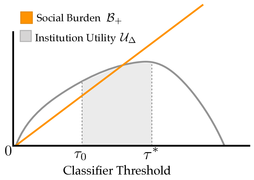
Figure 1 illustrates how institutional utility and social burden change as the threshold of the classifier increases. The institutional utility is quasiconcave, while the social burden is monotonically non-decreasing. The next lemma provides a formal characterization of the shapes shown in Figure 1.

Theorem 3.3.

The institutional utility $\mathcal{U}_{\Delta}(\tau)$ is quasiconcave in $\tau$ and has a maximum at a threshold $\tau^{*}\geq\tau_{0}$ where $\tau_{0}=0.5$ is the threshold of the non-strategic optimal classifier. The social burden $\mathcal{B}_{+}(\tau)$ is monotonically non-decreasing in $\tau$. Furthermore, if $\mathcal{U}_{\Delta}(\tau)\neq\mathcal{U}_{\Delta}(\tau^{\prime})$, then $\mathcal{B}_{+}(\tau)\neq\mathcal{B}_{+}(\tau^{\prime})$.

Proof.

Let $\mathcal{A}_{\Delta}(\tau)$ and $\mathcal{A}(\tau)$ be the set of individuals accepted by $f$ in the strategic and non-strategic setting, respectively. If $\tau<\tau_{0}$, we have $\mathcal{A}_{\Delta}(\tau)\supseteq\mathcal{A}_{\Delta}(\tau_{0})\supseteq\mathcal{A}(\tau_{0})$. Since $\mathcal{A}(\tau_{0})$ is the optimal non-strategic acceptance region, any $x\not\in\mathcal{A}(\tau_{0})$ has $\ell(x)<0.5$, and one can increase $\mathcal{U}_{\Delta}$ by not accepting $x$, which implies $\mathcal{U}_{\Delta}(\tau)\leq\mathcal{U}_{\Delta}(\tau_{0})$. Therefore, if a threshold $\tau^{*}$ is optimal for the institution, i.e. if $\mathcal{U}_{\Delta}(\tau^{*})=\max_{\tau}\mathcal{U}_{\Delta}(\tau)$, then $\tau^{*}\geq\tau_{0}$.

Recall that a univariate function $f(z)$ is quasiconcave if there exists $z^{*}$ such that $f$ is non-decreasing for $z<z^{*}$ and is non-increasing for $z>z^{*}$. Let $\tau^{*}$ be as above. For $\tau_{0}<\tau_{1}<\tau^{*}$, we have $\mathcal{A}_{\Delta}(\tau_{0})\supseteq\mathcal{A}_{\Delta}(\tau_{1})\supseteq\mathcal{A}_{\Delta}(\tau^{*})$. Since $\mathcal{U}_{\Delta}(\tau^{*})$ is optimal, $\mathcal{A}_{\Delta}(\tau^{*})$ is the optimal strategic acceptance region, and thus $\mathcal{U}_{\Delta}(\tau_{0})\leq\mathcal{U}_{\Delta}(\tau_{1})\leq\mathcal{U}_{\Delta}(\tau^{*})$. Similarly, if $\tau_{1}>\tau_{0}>\tau^{*}$ we have that $\mathcal{A}_{\Delta}(\tau^{*})\supseteq\mathcal{A}_{\Delta}(\tau_{0})\supseteq\mathcal{A}_{\Delta}(\tau_{1})$, and thus $\mathcal{U}_{\Delta}(\tau_{1})\leq\mathcal{U}_{\Delta}(\tau_{0})\leq\mathcal{U}_{\Delta}(\tau^{*})$. Therefore, $\mathcal{U}_{\Delta}(\tau)$ is quasiconcave in $\tau$.

The individual burden $b_{\tau}(x)=\min_{\ell(x^{\prime})\geq\tau}c(x,x^{\prime})$ is monotonically non-decreasing in $\tau$. Since the social burden $\mathcal{B}_{+}(\tau)$ is equal to $\mathbb{E}[b_{\tau}(x)\mid y=1]$, the social burden is also monotonically non-decreasing.

Suppose $\mathcal{U}_{\Delta}(\tau)\neq\mathcal{U}_{\Delta}(\tau^{\prime})$ and without loss of generality let $\tau<\tau^{\prime}$. For all individuals $x$, $b_{\tau^{\prime}}(x)\geq b_{\tau}(x)$. If there is at least one individual $x$ such that $b_{\tau^{\prime}}(x)>b_{\tau}(x)$, then $\mathcal{B}_{+}(\tau^{\prime})>\mathcal{B}_{+}(\tau)$. But since $\mathcal{U}_{\Delta}(\tau)\neq\mathcal{U}_{\Delta}(\tau^{\prime})$, there must exist an individual $x$ such that $x\in\mathcal{A}_{\Delta}(\tau)/\mathcal{A}_{\Delta}(\tau^{\prime})$ and $p(X=x\mid Y=1)>0$ since $\ell(x)>0$ by assumption. For this individual $b_{\tau^{\prime}}(x)>b_{\tau}(x)$. Therefore, $\mathcal{U}_{\Delta}(\tau)\neq\mathcal{U}_{\Delta}(\tau^{\prime})$ implies $\mathcal{B}_{+}(\tau^{\prime})\neq\mathcal{B}_{+}(\tau)$. ∎

As a corollary, if the institution increases its utility beyond that attainable by the optimal classifier in the non-strategic setting, then the institution also causes higher social burden.

Corollary 3.0.

Let $\tau$ be any threshold and $\tau_{0}=0.5$ be the optimal threshold in the non-strategic setting. If $\mathcal{U}_{\Delta}(\tau)>\mathcal{U}_{\Delta}(\tau_{0})$, then $\mathcal{B}_{+}(\tau)>\mathcal{B}_{+}(\tau_{0})$.

3.2. Choosing a Concrete Trade-off

The previous section shows increases in institutional utility come at a cost in terms of social burden and vice-versa. This still leaves open the question: what is the concrete trade-off an institution should choose?

Theorem 3.3 provides a precise characterization of the choices available to trade-off between institutional utility and social burden. The baseline choice for the institution is to not account for strategic behavior and use the non-strategic optimum $\tau_{0}$. Maximizing utility without regard to social burden leads the institution to choose $\tau^{*}$. In general, the interval $[\tau_{0},\tau^{*}]$ offers the set of trade-offs the institution considers. Choosing $\tau>\tau_{0}$ can increase robustness at the price of increasing social burden. Thresholds $\tau>\tau^{*}$ are not Pareto-efficient and are not considered.

Much of the prior work in machine learning has focused exclusively on solutions corresponding to the thresholds at the extreme: $\tau_{0}$ and $\tau^{*}$. The threshold $\tau_{0}$ is the solution when strategic behavior is not accounted for. The threshold $\tau^{*}$ is also known as the Stackelberg equilibrium and is the subject of recent work in strategic classification (Brückner and Scheffer, 2011; Hardt et al., 2016a; Dong et al., 2018). While using $\tau^{*}$ may be warranted in some cases, a proper accounting of social burden would lead institutions to choose classifiers somewhere between the extremes of $\tau_{0}$ and $\tau^{*}$.

The exact choice of $\tau\in[\tau_{0},\tau^{*}]$ is context-dependent and depends on balancing concerns between institutional and broader social interest. We now highlight cases where using $\tau_{0}$ or $\tau^{*}$ may be suboptimal, and using a threshold $\tau\in(\tau_{0},\tau^{*})$ that balances robustness with social burden is preferable.

Example 3.0 (Expensive features.).

If measuring a feature is costly for individuals and offers limited gains in predictive accuracy, an institution may choose to ignore the feature, even if it means giving up accuracy on the margin. In an educational context, a university may decide to no longer require applicants to submit standardized test scores, which can cost applicants hundreds of dollars, if the corresponding improvement in admissions outcomes is very small (pri, 2018).

Example 3.0 (Reducing social burden under resource constraints.).

Aid organizations increasingly use machine learning to determine where to allocate resources after natural disasters (Imran et al., 2014). In these cases, positive individuals are precisely those people who are in need of aid and may experience very high costs to change their features. Using thresholds with high social burden is therefore undesirable. At the same time, aid organizations often face significant resource constraints. False positives from individuals gaming the classifier ties up resources that could be better used elsewhere. Consequently, using the non-strategic threshold is also undesirable. The aid organization should choose a some threshold $\tau$ with $\tau_{0}<\tau<\tau^{*}$ that reflects these trade-offs.

Example 3.0 (Misspecification of agent model.).

Strategic classification models typically assume the individual optimally responds to the classifier $f$. In reality, individuals will not have perfect knowledge of the classifier $f$ when it is first deployed. Instead, they may be able to learn about how the classifier works over time, and gradually improve their ability to game the classifier. For example, self-published romance authors exchanged information in private chat groups about how to best game Amazon’s book recommendation algorithms (Jeong, 2018). For the institution, it is difficult to a priori model the dynamics of how information about the classifier propagates. A preferable solution may be to simply make the assumption that the individual can best respond to the classifier, but to only gradually increase the threshold from the non-strategic $\tau_{0}$ to the Stackelberg optimal $\tau^{*}$ over time.

In fact, misspecification of the agent model (described above), is why Brückner et al. (2012) suggest the Stackelberg equilibrium is too conservative, and instead prefer to use Nash equilibrium strategies. Complementary to their observation, we show that there is a more general reason Nash equilibria may be preferable. Namely, that Nash equilibria have lower social burden than the Stackelberg solution. As the following lemma shows, in our context, the set of Nash equilibria form an interval $[t_{N},\tau^{*}]\subset I$ for some $t_{N}\geq t_{0}$. The proof is deferred to the appendix.

Lemma 3.0.

Suppose the cost over likelihoods $c_{L}$ is continuous and $\ell(\mathcal{X})=[0,1]$, i.e, all likelihoods have non-zero support. Then, the set of Nash equilibrium strategies for the institution is $[\tau_{N},\tau^{*}]$ for some $\tau_{N}\geq\tau_{0}$ where $\tau_{0}=0.5$ is the non-strategic optimal threshold and $\tau^{*}$ is the Stackelberg equilibrium strategy.

The Stackelberg equilibrium requires the institution to choose $\tau^{*}$, whereas Nash equilibria give the institution latitude to trade-off between institutional utility and social burden by choosing from the interval $[t_{N},\tau^{*}]\subset I$. This provides an additional argument in favor of Nash equilibria– institutions can still reason in terms of equilibria and achieve more favorable outcomes in terms of social burden.

4. Fairness to Subpopulations

Our previous section showed that increased robustness in the face of strategic behavior comes at the price of additional social burden. In this section, we show this social burden is not fairly distributed: when the individuals being classified are from latent subpopulations, say of race, gender, or socioeconomic status, the social burden can disproportionately fall on disadvantaged subpopulations. Furthermore, we find that improving the institution’s utility can exacerbate the gap between the social burden incurred by an advantaged and disadvantaged group.

Concretely, suppose each individual is from a subpopulation $g\in\{a,b\}$. The social burden a classifier $f$ has on a group $g$ is the expected minimum cost required for a positive individual from group $g$ to be accepted: $\mathcal{B}_{+,g}(f)=\mathbb{E}\left[\min_{x^{\prime}:f(x^{\prime})=1}c(x,x^{\prime})\mid Y=1,G=g\right]$. We can then define the social gap between groups $a$ and $b$:

Definition 4.0 (Social gap).

The social gap $\mathcal{G}(f)$ induced by a classifier $f$ is the difference in the social burden to group $b$ compared to $a$: $\mathcal{G}(f)=\mathcal{B}_{+,b}(f)-\mathcal{B}_{+,a}(f)$.

The social gap is a measure of how much more costly it is for a positive individual from group $b$ to be accepted by the classifier than a positive individual from group $a$. For example, there is evidence that women need to attain higher educational qualifications than their male counterparts to receive the same salary (Carnevale et al., 2018).

A high social gap is alarming for two reasons. First, even when two people from group $a$ and group $b$ are equally qualified, the individual from group $a$ may choose not to participate at all because of the cost she would need to endure to be accepted. Secondly, if she does decide to participate, she may continue to be at a disadvantage after being accepted because of the additional cost she had to endure, e.g., repaying student loans.

Non-strategic classification can already induce a social gap between two groups, and strategic classification can exacerbate this gap. We show this under two natural ways group $b$ may be disadvantaged. In the first setting, the feature distributions of group $a$ and $b$ are such that a positive individual from group $b$ is less likely to be considered positive, compared to group $a$. In the second setting, individuals from group $b$ have a higher cost to adapt their features compared to group $a$. Under both of these conditions, any improvement the institution can make to its own strategic utility has the side effect of worsening (increasing) the social gap.

4.1. Different Feature Distributions

In the first setting we analyze, the way groups $a$ and $b$ differ is through their distributions over features. We say that group $b$ is disadvantaged if the features distributions are such that positive individuals from group $b$ are less likely to be considered positive than those from group $a$. Formally, this can be characterized as the following:

Definition 4.0 (Disadvantaged in features).

Let $L_{+,g}=\ell(X)\mid Y=1,G=g$ be the outcome likelihood of a positive individual from group $g$, and let $F_{+,g}$ be the cumulative distribution function of $L_{+,g}$. We say that group $b$ is disadvantaged in features if $F_{+,b}(l)>F_{+,a}(l)$ for all $l\in(0,1)$.

In the economics literature, the relationship between $L_{+,a}$ and $L_{+,b}$ is referred to as strict first-order stochastic dominance (Levy, 1992). Intuitively, that group $b$ is disadvantaged in features if and only if the distribution of $L_{+,a}$ can be transformed to the distribution of $L_{+,b}$ by transferring probability mass from higher values to lower values. This definition captures the notion that the outcome likelihood of positive individuals from group $b$ is skewed lower than the outcome likelihood of positive individuals from $a$.

In a case study on FICO credit scores in Section 5, we find the minority group (blacks) is disadvantaged in features compared to the majority group (whites) (see Figure 2). There are many reasons that a group could be disadvantaged in features. Below, we go through a few potential causes.

Example 4.0 (Group membership explains away features).

Even if two groups are equally likely to have positive individuals, i.e., $\mathbb{P}(Y=1\mid G=a)=\mathbb{P}(Y=1\mid G=b)$, group $b$ can still be disadvantaged compared to group $a$. Consider the graph below. Although the label $Y$ is independent of the group $G$, the label $Y$ is not independent of the group $G$ once conditioned on the features $X$ because the group $G$ can provide an alternative reason for the observed features.

Concretely, let groups $a$ and $b$ be native and non-native speakers of english, $X$ be the number of grammatical errors on an individual’s job application, and $Y$ be whether the individual is a qualified candidate. Negative individuals ($Y=0$) are less meticulous when filling out their application and more likely to have grammatical errors. However, for individuals from group $b$ there is another explanation for having grammatical errors – being a non-native speaker. Thus, positive individuals from group $b$ end up with lower outcome likelihoods than those from $a$, even though they may be equally qualified.

Example 4.0 (Predicting base rates).

Suppose the rate of positives in group $b$ is lower than that of group $a$: $\mathbb{P}(Y=1\mid G=b)<\mathbb{P}(Y=1\mid G=a)$. If there is a feature in the dataset that can be used as a proxy for predicting the group, such as zip code or name for predicting race, then the outcome likelihoods of positive individuals from group $b$ can end up lower than those of positive individuals from group $a$ because the features are simply predicting the base rate of each group.

Social gap increases.

We now state and prove the main result showing that the social gap increases as the institution increases its threshold for acceptance. Before turning to the result, we introduce one technical requirement. The likelihood condition is that $\frac{\partial c_{L}(l,\tau)}{\partial l}$ is monotonically non-increasing in $\tau$ for $l,\tau\in[0,1]$. When the cost function $c$ is outcome monotonic, the likelihood condition is satisfied for a broad class of differentiable likelihood cost functions $c_{L}$, such as the following examples.

• Differentiable separable cost functions of the form $c_{L}(l,l^{\prime})=\max(c_{2}(l^{\prime})-c_{1}(l),0)$ for $c_{1},c_{2}:[0,1]\rightarrow\mathbb{R}_{\geq 0}$.

• Differentiable shift-invariant cost functions of the form

  $$c_{L}(l,l^{\prime})=\begin{cases}c_{0}(l^{\prime}-l)&l<l^{\prime}\\ 0&l\geq l^{\prime}\end{cases}\,,$$

  for convex $c_{0}:[0,1]\rightarrow\mathbb{R}_{\geq 0}$.

Notably, any linear cost $c_{L}(l,l^{\prime})=\max(\alpha(l^{\prime}-l),0)$ where $\alpha>0$ satisfies the likelihood condition.

Under the likelihood condition, we now show that the social gap increases as the institution increases its threshold for acceptance.

Theorem 4.5.

Let $\tau\in(0,1]$ be the threshold of the classifier. If group $b$ is disadvantaged in features compared to group $a$, and $\frac{\partial c_{L}(l,\tau)}{\partial l}$ is monotonically non-increasing in $\tau$, then $\mathcal{G}(\tau)$ is positive and monotonically increasing over $\tau$.

Proof.

By Lemma 2.4, any outcome monotonic cost function can be written as a cost over outcome likelihoods. Therefore, the social burden can be written as

$$\mathcal{B}_{+,g}(\tau) =\mathbb{E}\left[c_{L}(\ell(x),\tau)\mid Y=1,G=g\right]$$

$$=\int_{0}^{\tau}c_{L}(l,\tau)\mathop{}\!\mathrm{d}F_{+,g}(l),$$

where $F_{+,g}$ denotes the CDF of the group outcome likelihood $L_{+,g}$. Integrating by parts, we obtain a simple expression for $\mathcal{B}_{+,g}(\tau)$:

$$\mathcal{B}_{+,g}(\tau) =\int_{0}^{\tau}c_{L}(l,\tau)\mathop{}\!\mathrm{d}F_{+,g}(l)$$

$$=[c_{L}(l,\tau)F_{+,g}(l)]^{\tau}_{0}-\int_{0}^{\tau}\frac{\partial c_{L}(l,\tau)}{\partial l}F_{+,g}(l)\mathop{}\!\mathrm{d}l$$

$$=-\int_{0}^{\tau}\frac{\partial c_{L}(l,\tau)}{\partial l}F_{+,g}(l)\mathop{}\!\mathrm{d}l\,,$$

where the last line follows because $c_{L}(\tau,\tau)=0$ and $F_{+,g}(0)=0$. This expression for $\mathcal{B}_{+,g}(\tau)$ allows us to conveniently write the social gap as

$$\mathcal{G}(\tau)=\mathcal{B}_{+,b}(\tau)-\mathcal{B}_{+,a}(\tau)=\int_{0}^{\tau}\frac{\partial c_{L}(l,\tau)}{\partial l}(F_{+,a}(l)-F_{+,b}(l))\mathop{}\!\mathrm{d}l\,.$$

We now argue the social gap $\mathcal{G}(\tau)$ is positive. By the monotonicity assumptions, $\frac{\partial c_{L}(l,\tau)}{\partial l}<0$ for $l\in(0,\tau)$. Since group $b$ is disadvantaged in features, $F_{+,a}(l)-F_{+,b}(l)<0$ for $l\in(0,1)$. Therefore, $\mathcal{G}(\tau)>0$.

Now, we show $\mathcal{G}(\tau)$ is increasing in $\tau$. Let $0\leq\tau<\tau^{\prime}\leq 1$. Then, the difference in the social gap is given by

$$\mathcal{G}(\tau^{\prime})-\mathcal{G}(\tau) =\int_{0}^{\tau}\frac{\partial\left(c_{L}(l,\tau^{\prime})-c_{L}(l,\tau)\right)}{\partial l}(F_{+,a}(l)-F_{+,b}(l))\mathop{}\!\mathrm{d}l$$

$$+\int_{\tau}^{\tau^{\prime}}\frac{\partial c_{L}(l,\tau^{\prime})}{\partial l}(F_{+,a}(l)-F_{+,b}(l))\mathop{}\!\mathrm{d}l.$$

Since group $b$ is disadvantaged in features, $(F_{+,a}(l)-F_{+,b}(l))<0$ for all $l$. By assumption, $\frac{\partial c_{L}(l,\tau)}{\partial l}$ is monotonically non-increasing in $\tau$, so the first term is non-negative. Similarly, $\frac{\partial c_{L}(l,\tau^{\prime})}{\partial l}<0$ by monotonicity, so the second term is positive. Hence, $\mathcal{G}(\tau^{\prime})-\mathcal{G}(\tau)>0$, which establishes $\mathcal{G}(\tau)$ is monotonically increasing in $\tau$. ∎

As a corollary, if the institution improves its utility beyond the non-strategic optimal classifier, then it also causes the social gap to increase.

Corollary 4.0.

Suppose group $b$ is disadvantaged in features compared to group $a$, and $\frac{\partial c_{L}(l,\tau)}{\partial l}$ is monotonically non-decreasing in $\tau$. Let $\tau\in(0,1]$ be a threshold and $\tau_{0}=0.5$ be the optimal non-strategic threshold. If $\mathcal{U}_{\Delta}(\tau)>\mathcal{U}_{\Delta}(\tau_{0})$, then $\mathcal{G}(\tau)>\mathcal{G}(\tau_{0})$.

Proof.

By Theorem 3.3, if $\mathcal{U}_{\Delta}(\tau)>\mathcal{U}_{\Delta}(\tau_{0})$, then $\tau>\tau_{0}$. By Theorem 4.5, if $\tau>\tau_{0}$, then $\mathcal{G}(\tau)>\mathcal{G}(\tau_{0})$. ∎

4.2. Different Costs

In Section 4.1, we showed that when two subpopulations have different feature distributions, the social burden can disproportionately fall on one group. In this section, we show that even if the feature distributions of the two groups are exactly identical, the social burden can still disproportionately impact one group.

We have thus far assumed the existence of a cost function $c$ that is uniform across groups $a$ and $b$. For a variety of structural reasons, it is unlikely this assumption holds in practice. Rather, it is often the case that different groups experience different costs for changing their features.

When the cost for group $b$ is systematically higher than the cost for group $a$, we prove group $b$ incurs higher social burden than group $a$. Furthermore, if the institution improves its utility by increasing its threshold $\tau$, then as a side effect it also increases the social gap between group $b$ and $a$ (Theorem 4.11).

Much of the prior work on fairness in classification focuses on preventing unfairness that can arise when different subpopulations have different distributions over features and labels (dwork2012fairness; Hardt et al., 2016b; Chouldechova, 2017). Our result provides a reason to be concerned about the unfair impacts of a classifier even when two groups have identical initial distributions. Namely, that it can be easier for one group to game the classifier than another.

Formally, we say that group $b$ is disadvantaged in cost compared to group $a$ if the following condition holds.

Definition 4.0 (Disadvantaged in cost).

Let $c_{g}(x,x^{\prime})$ be the cost for an individual from group $g$ to adapt their features from $x$ to $x^{\prime}$. Group $b$ is disadvantaged in cost if $c_{b}(x,x^{\prime})=\kappa c_{a}(x,x^{\prime})$ for all $x,x^{\prime}\in X$ and some scalar $\kappa>1$.

Next, we give a variety of example scenarios of when a group can be disadvantaged in cost.

Example 4.0 (Opportunity Costs).

Many universities have adopted gender-neutral policies that stop the “tenure-clock” for a year for family-related reasons, e.g. childbirth. Ostensibly, no research is expected while the clock is stopped. However, the adoption of gender-neutral clocks actually increased the gap between the percentage of men and women who received tenure (Antecol et al., ming). The suggested cause is that women still shoulder more of the burden of bearing and caring for children, compared to men. Men who stop their tenure clock are more productive during the period than women, who have a higher opportunity cost to doing research while raising a child.

Example 4.0 (Information Asymmetry).

A large portion of high-achieving, low-income students do not apply to selective colleges, despite the fact that these colleges are typically less expensive for them because of the financial aid they would receive (Hoxby and Avery, 2012). This phenomenon seems to be due to low-income students having less access to information about college (hoxby2013expanding). Since low-income students have more barriers to gaining information about college, it is natural to assume that, compared to their wealthier peers, they have a higher cost to strategically manipulating their admission features.

Example 4.0 (Economic Differences).

Consider a social media company that wishes to classify individuals as “influencers,” either to more widely disseminate their content or to identify promising accounts for online marketing campaigns. Wealthy individuals can purchase followers or likes, whereas other groups have to increase these numbers organically (Chafkin, 2016). Consequently, the costs to increasing one’s popularity metric differs based on access to capital.

Finally, our main technical result shows that even when the distributions of groups $a$ and $b$ are identical, if group $b$ is disadvantaged in cost, then when the institution increases its threshold for acceptance, it also increases the social gap between the two groups.

Theorem 4.11.

Suppose positive individuals from groups $a$ and $b$ have the same distribution over features, i.e, if $Z=\left(X\mid Y=1\right)$, then $Z$ is independent of the group $G$. If group $b$ is disadvantaged in cost compared to group $a$, then the social gap $\mathcal{G}(\tau)$ is non-negative and monotonically non-decreasing in the threshold $\tau$.

Proof.

Since $X\mid Y=1$ is independent of $G$, the social burden to a group $g$ can be written as

$$\mathcal{B}_{+,g}(\tau)=\int_{\mathcal{X}}\min_{x^{\prime}:f_{\tau}(x^{\prime})=1}c_{g}(x,x^{\prime})p(X=x\mid Y=1)\mathop{}\!\mathrm{d}x$$

where $f_{\tau}$ is the outcome likelihood classifier with threshold $\tau$. The social gap can then be expressed as

$$\mathcal{G}(\tau) =\mathcal{B}_{+,b}(\tau)-\mathcal{B}_{+,a}(\tau)$$

$$=\int_{\mathcal{X}}(\kappa-1)\min_{x^{\prime}:f_{\tau}(x^{\prime})=1}c_{a}(x,x^{\prime})~{}p(X=x\mid Y=1)\mathop{}\!\mathrm{d}x\,$$

$$=(\kappa-1)\mathcal{B}_{+,a}(\tau).$$

Since the group social burden $\mathcal{B}_{+,a}(\tau)$ is non-negative and monotonically non-decreasing, the social gap $\mathcal{G}(\tau)$ is also non-negative and monotonically non-decreasing. ∎

5. Case Study: FICO Credit Data

We illustrate the impact of strategic classification on different subpopulations in the context of credit scoring and lending. FICO scores are widely used in the United States to predict credit worthiness. The scores themselves are derived from a proprietary classifier that uses features that are susceptible to gaming and strategic manipulation, for instance the number of open bank accounts.

We use a sample of 301,536 FICO scores derived from TransUnion TransRisk scores (Reserve, 2007) and preprocessed by Hardt et al. (2016b). The scores $X$ are normalized to lie between 0 and 100. An individual’s outcome is labeled as a default if she failed to pay a debt for at least 90 days on at least one account in the ensuing 18-24 month period. Default events are labeled with $Y=0$, and otherwise repayment is denoted with $Y=1$. The two subpopulations are given by race: $a=\text{\tt white}$ and $b=\text{\tt black}$.

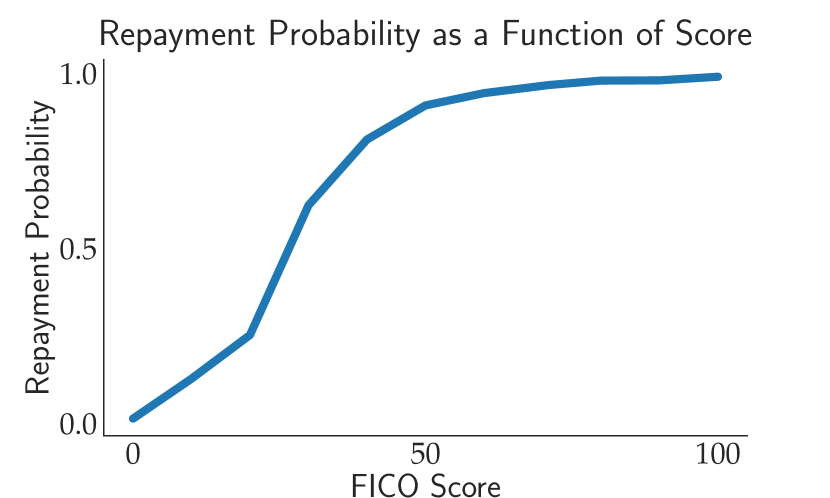
We assume the credit lending institution accepts individuals based on a threshold on the FICO score. Using the normalized scale, a threshold of $\tau=58$ is typically used to determine eligibility for prime rate loans (Hardt et al., 2016b). Our results thus far have used thresholds on the outcome likelihood, rather than a score. However, as shown in Figure 3, the outcome likelihood is monotonic in the FICO score. Therefore, all our conditions and results can be validated using the score instead of the outcome likelihood.

5.1. Different Feature Distributions

In Section 4.1, we studied the scenario where the distribution of outcome likelihoods $\ell(X)=\mathbb{P}(Y=1\mid X)$ differed across subpopulations. In particular, if the likelihoods of the positive individuals in group $B$ tend to be lower than the positive individuals in group $A$, then increasing strategic robustness increases the social gap between $A$ and $B$.

Interestingly, such a skew in score distributions exists in the FICO data. Black borrowers who repay their loans tend to have lower FICO scores than white borrowers who repay their loans. In terms of the corresponding score CDFs, for every score $x$, $F_{+,\tt black}(x)\geq F_{+,\tt white}(x)$. Figure 2 demonstrates this observation.

Figure 2. Comparison of the distribution of FICO scores among black and white borrowers who repaid their loans. Credit-worthy black individuals tend to have lower credit scores than credit-worthy white individuals. The comparison of the corresponding CDFs demonstrates our “disadvantaged in features” assumption holds.

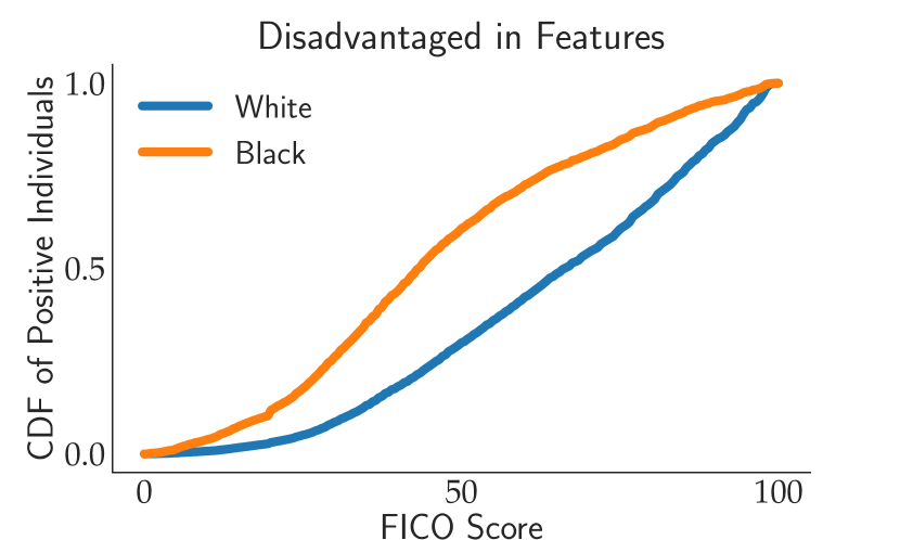
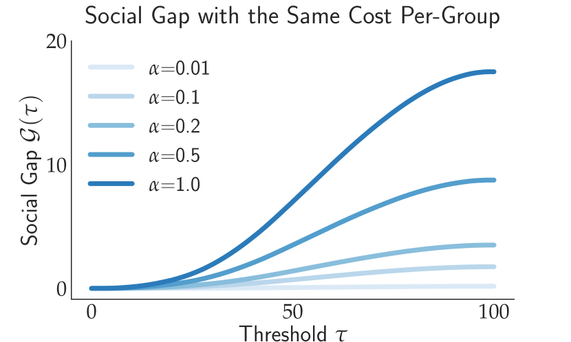
When the score distribution among positive individuals is skewed, Theorem 4.5 guarantees the social gap between groups is increasing in the threshold under a reasonable cost model. Operationally, raising the loan threshold to protect against strategic behavior increases the relative burden on the black subgroup. To demonstrate this empirically, we use a coarse linear cost model, $c(x,x^{\prime})=\max(\alpha(x^{\prime}-x),0)$ for some $\alpha>0$. Here, $\alpha$ corresponds to the cost of raising one’s FICO score one point. Since the probability of repayment $\mathbb{P}(Y=1\mid x)$ is monotonically increasing in $x$, the linear cost $c$ satisfies the requisite outcome monotonicity conditions.

Figure 3. Repayment probability as a function of credit score. Crucially, the probability of repayment $\mathbb{P}(Y=1\mid x)$ is monotonically increasing in $x$.

In Figure 4, we compute $\mathcal{G}(\tau)$ as $\tau$ varies from $0$ to $100$ for a range of different value of $\alpha$. For any $\alpha$, the social utility gap is increasing in $\tau$. Moreover, as $\alpha$ becomes large, the rate of increase in the social gap grows large as well.

Figure 4. Impact of increasing the threshold $\tau$ on white and black credit applicants. When the cost to changing one’s score $\alpha$ is small, increases to the threshold have only a small effect on the social gap. However, as $\alpha$ becomes large, even small increases to the threshold can create large discrepancies in social burden between the two groups.

5.2. Different Cost Functions

In Section 4.2, we demonstrated when two subpopulations are identically distributed, but incur different costs for changing their features, there is a non-trivial social gap between the two. In the context of the FICO scores, it is plausible that blacks are both disadvantaged in features and experience higher costs for changing their scores. For instance, outstanding debt is an important component of FICO scores. One way to reduce debt is to increase earnings. However, a persistent black-white wage gap between the two subpopulations suggest increasing earnings is easier for group $a$ than group $b$ (Daly et al., 2017). This setting is not strictly captured by our existing results, and we should expect the effects of both different costs functions and different feature distributions to compound and exacerbate the unfair impacts of strategic classification.

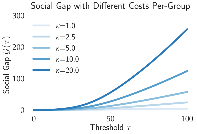
To illustrate this phenomenon, we again use a coarse linear cost model. Suppose group A has cost $c_{A}(x,x^{\prime})=\max\{\alpha(x^{\prime}-x),0\}$ for some $\alpha>0$, and group B has cost $c_{B}(x,x^{\prime})=\max\{\beta(x^{\prime}-x),0\}$ for some $\beta\geq\alpha$. As in Section 4.2, group B is disadvantaged in cost provided the ratio $\kappa=\beta/\alpha>1$. In Figure 5, we show the social gap $\mathcal{G}(\tau)$ for various settings of $\kappa$. The social gap is always increasing as a function of $\tau$, and the rate of increase grows large for even moderate values of $\kappa$. When $\kappa$ is large, even small increases in $\tau$ can disproportionately increase the social burden for the disadvantaged subpopulation.

Figure 5. Impact of increasing the threshold $\tau$ on white and black credit applicants, under the assumption that both groups incur different costs for increasing their credit score. As the ratio between the costs $\kappa$ increases, the social cost gap grows rapidly between the two groups.

6. Related Work

Strategic Classification

Prior work on strategic classification focuses solely on the institution, primarily aiming to create high-utility solutions for the institution. Our work, on the other hand, studies the tradeoff between the institution’s utility and the burden to the individuals being classified.

Hardt et al. (2016a); Dong et al. (2018); Brückner and Scheffer (2011) give algorithms to compute the Stackelberg equilibrium, which corresponds to the extreme $\tau^{*}$ solution in our trade-off curves. Although the Stackelberg equilibrium leads to maximal institutional utility, we show that it also causes high social burden. We give several examples of when the high social burden induced by the Stackelberg equilibrium makes it an undesirable solution for the institution.

Rather than the Stackelberg equilibrium, others have also considered finding Nash equilibria of the game  (Brückner et al., 2012; Dalvi et al., 2004).  Brückner et al. (2012) argue that since in practice people cannot optimally respond to the classifier, the Stackelberg solution tends to be too conservative, and thus a Nash equilibrium strategy is preferable. Our work provides a complementary reason to prefer Nash equilibria over the Stackelberg solution. Namely, for a broad class of cost functions, any Nash equilibrium that is not equal to the Stackelberg equilibrium places lower social burden on individuals.

Finally, we focus on the setting where individuals are merely “gaming” their features, i.e., they do not improve their true label by adapting their features. However, if the classifier is able to incentivize strategic behavior that helps improve negative individuals, then the social burden placed on positive individuals may be considered acceptable.  Kleinberg and Raghavan (2018) studies how to design classifiers that produce such incentives.

Fairness

Our work studies how strategic classification results in differing impacts to different subpopulations and is complementary to the large body of work studying the differing impacts of classification (of the President et al., 2016; Barocas and Selbst, 2016).

The prior work on classification is primarily concerned with preventing unfairness that can arise due to subpopulations having differing distributions over features or labels (Hardt et al., 2016b; dwork2012fairness; Chouldechova, 2017). We show that in the strategic setting, a classifier can have differing impact due to the subpopulations having differing distributions or differing costs to adapting their features. Therefore, when individuals are strategic, our work provides an additional reason to be concerned about the fairness of a classifier. In particular, it can be easier for one group to game the classifier than another.

Furthermore, we show that if the institution modifies the classifier it uses to be more robust to strategic behavior, then it also as a side effect, increases the gap between the cost incurred by a disadvantaged subpopulation and an advantaged population. Thus, strategic classification can exacerbate unfairness in classification.

Our work is also complementary to Liu et al. (2018), who also analyze how the institution’s utility trades-off with the impact to individuals. They study the trade-off in the non-strategic setting and measure the impact of a classifier using a dynamics model of how individuals are affected by the classification they receive. We study the tradeoff in the strategic setting and measure the impact of a classifier by the cost of the strategic behavior induced by the classifier.

In concurrent work, hu2018disparate also study negative externalities of strategic classification. In their model, they show that the Stackelberg equilibrium leads to only false negative errors on a disadvantaged population and false positives on the advantaged population. Furthermore, they show that providing a cost subsidy for disadvantaged individuals can lead to worse outcomes for everyone.

7. Discussion of Social Burden

To measure the impact of strategic classification on the individuals being classified, we introduced a measure of social burden, defined as the expected cost that positive individuals need to incur to be classified positively: $\mathcal{B}_{+}(f)=\mathbb{E}\left[\min_{f(x^{\prime})=1}c(x,x^{\prime})\mid y=1\right]$. An alternative measure one might consider is the expected individual utility for the positives: $\mathcal{S}_{+}(f)=\mathbb{E}\left[u_{x}(f,\Delta(x))\mid y=1\right]$, which we will denote the social utility.

We prefer social burden to social utility because it makes fewer assumptions about individual behavior. Social utility measures the utility of the individual while assuming that they respond optimally and needs the assumption to hold to be a meaningful measure. Social burden, on the other hand, applies irrespective of the different policies individuals may actually act according to. Our analysis assumes the institution assumes individuals respond optimally, but we ourselves believe this to be a strong assumption to hold in practice, and would like our measure of impact on individuals to apply regardless.

Moreover, most of our results are agnostic to the specific choice of social cost measure. The results in Section 3 about the tradeoff between institutional utility and social burden all still hold. Specifically, Theorem 3.3 holds with social utility instead of social burden (and monotonically non-increasing instead of monotonically non-decreasing since lower utility is worse). For our results in Section 4, i.e, Theorems 4.5 and 4.11, there is still always a non-negative social gap (now defined as the difference in social utilities between the groups), but it is not necessarily true that the social gap increases as the institution’s threshold increases.

While both social burden and social utility apply only to positive individuals, one could also use versions that integrate over all individuals: $\mathcal{B}(f)=\mathbb{E}\left[\min_{f(x^{\prime})=1}c(x,x^{\prime})\right]$ and $\mathcal{S}(f)=\mathbb{E}\left[u_{x}(f,\Delta(x))\right]$. Our results for $\mathcal{B}_{+}(f)$ go through for $\mathcal{B}(f)$, and the results for $\mathcal{S}_{+}(f)$ go through for $\mathcal{S}(f)$. However, in many cases giving a positive classification (e.g. a loan) to a negative individual (someone who will default) can result in a long-term negative impact to that individual (Liu et al., 2018). In general, it is uncertain whether the reducing the costs incured by the negative individuals confers positive social benefits, and we do not incorporate these costs into our measure.

Overall, there are many potential measures that are complementary to our measure of social burden, but they all provide a similar takeaway. Namely, that in the strategic setting, there is a tradeoff between institutional accuracy and individual impact that must be considered when making choices about strategy-robustness.

8. Acknowledgements

This material is based upon work supported by the National Science Foundation Graduate Research Fellowship Program under Grant No. DGE 1752814. Any opinions, findings, and conclusions or recommendations expressed in this material are those of the author(s) and do not necessarily reflect the views of the National Science Foundation.

Appendix A Proof of Lemma 3.8

Proof.

The lemma follows by proving the following properties about the Nash equilibrium strategies for the institution.

• The Stackelberg threshold $\tau^{*}$ is a Nash equilibrium strategy.

• All Nash equilibrium strategies lie in the interval $[\tau_{0},\tau^{*}]$.

• If $\tau_{N}$ is a Nash equilibrium strategy, then all $\tau\in[\tau_{N},\tau^{*}]$ are also Nash equilibrium strategies.

Together, the three properties imply that the set of institution equilibrium strategies is $[\tau_{N},\tau^{*}]$ for some $\tau_{N}\in[\tau_{0},\tau^{*}]$.

Before proceeding, we first establish and recall a few definitions. Let $\Delta_{\tau}(x)$ be the best response of individual $x$ to the threshold $\tau$. Define the set of individuals accepted for threshold $\tau$ and response $\Delta_{\tau}$ by $\mathcal{A}_{\Delta_{\tau}}(\tau)=\{x:f_{\tau}(\Delta_{\tau}(x))=1\}$. Recall the outcome likelihood $\ell(x)=\mathbb{P}(Y=1\mid X=x)$. Define the strategic outcome likelihood as $\ell_{\Delta_{\tau}}(x^{\prime})=\mathbb{P}(Y=1\mid\Delta_{\tau}(X)=x^{\prime})$. The outcome likelihood is the probability that an individual is positive given their true features, while the strategic outcome likelihood is the probability that an individual is positive given their gamed features.

For the pair $(\tau,\Delta_{\tau})$ to be a Nash equilibrium, $\tau$ must be a best response to the individual’s best response $\Delta_{\tau}(x)$. With knowledge of the individual’s response, $x^{\prime}=\Delta_{\tau}(x)$, the institution’s best response is to play a threshold $\tau^{\prime}$ so that $x^{\prime}\in\mathcal{A}_{\Delta_{\tau}}(\tau^{\prime})$ iff $\ell_{\Delta_{\tau}}(x^{\prime})\geq 0.5$. Therefore, to show $(\tau,\Delta_{\tau})$ is a Nash equilibrium, we must show $\tau=\tau^{\prime}$, i.e. $x^{\prime}\in\mathcal{A}_{\Delta_{\tau}}(\tau)$ iff $\ell_{\Delta_{\tau}}(x^{\prime})\geq 0.5$.

To verify the condition $x^{\prime}\in\mathcal{A}_{\Delta_{\tau}}(\tau)$ iff $\ell_{\Delta_{\tau}}(x^{\prime})\geq 0.5$, there are three cases to consider.

1. If $\ell(x)>\tau$, then $x\in\mathcal{A}_{\Delta_{\tau}}(\tau)$, $\Delta_{\tau}(x)=x$, and $\ell_{\Delta_{\tau}}(x)=\ell(x)$. Therefore, it suffices to check $\ell(x)\geq 0.5$.

2. If $\ell(x)<\tau$ and $c_{L}(\ell(x),\tau)>1$, then $x\not\in\mathcal{A}_{\Delta_{\tau}}(\tau)$ and $\Delta_{\tau}(x)=x$. In this case, it suffices to check $\ell(x)<0.5$.

3. If $\ell(x)<\tau$ and $c_{L}(\ell(x),\tau)\leq 1$, then $\Delta_{\tau}(x)\in\mathcal{A}_{\Delta_{\tau}}(\tau)$, but $x\neq\Delta_{\tau}(x)$, so we must directly verify $\mathbb{P}(Y=1\mid c_{L}(\ell(X),\tau)\leq 1,\ell(X)\leq\tau)\geq 0.5$.

We now proceed to the proof.

First, we show the Stackelberg equilibrium $(\tau^{*},\Delta_{\tau^{*}})$ is a Nash equilibrium. The Stackelberg threshold $\tau^{*}$ is the largest $\tau^{*}$ such that $c_{L}(0.5,\tau^{*})\leq 1$. If $\ell(x)>\tau^{*}$, by monotonicity, $\ell(x)\geq 0.5$. If $\ell(x)<\tau^{*}$ and $c_{L}(\ell(x),\tau^{*})>1$, then $\ell(x)<0.5$ by definition of $\tau^{*}$. Similarly, if $\ell(x)<\tau^{*}$ and $c_{L}(\ell(x),\tau^{*})\leq 1$, then $\ell(x)\geq 0.5$, so trivially $\mathbb{P}(Y=1\mid c_{L}(\ell(X),\tau)\leq 1,\ell(X)\leq\tau)\geq 0.5$. Hence, $(\tau^{*},\Delta_{\tau^{*}})$ is a Nash equilibrium.

Next, we show that all Nash strategies must lie in the interval $[\tau_{0},\tau^{*}]$.

1. Suppose $\tau<\tau_{0}=0.5$. For all $x$ such that $\ell(\Delta_{\tau}(x))=\tau$, $\ell(x)<0.5$. Therefore, $\mathbb{P}(Y=1\mid c_{L}(\ell(X),\tau)\leq 1,\ell(X)\leq\tau)<0.5$, so $\tau$ cannot be a Nash equilibrium strategy for the institution.

2. Suppose $\tau>\tau^{*}$. By definition, $\tau^{*}$ is the largest $\tau$ such that $c_{L}(0.5,\tau)\leq 1$. Thus, if $\tau>\tau^{*}$, there exists $x$ with $\ell(x)<\tau^{*}$ and $c_{L}(\ell(x),\tau)>1$, but $\ell(x)\geq 0.5$. Hence, $\tau$ cannot be a Nash strategy.

Finally, we show that if $\tau_{N}$ is a Nash equilibrium strategy, then so is $\tau$ for any $\tau\in[\tau_{N},\tau^{*}]$. We consider each of the three cases in turn.

1. Suppose $\ell(x)>\tau$. Then $\ell(x)>\tau>\tau_{N}\geq\tau_{0}=0.5$.

2. Suppose $\ell(x)<\tau$ and $c_{L}(\ell(x),\tau)>1$. Since $\tau\leq\tau^{*}$, by monotonicity in the second argument, $c_{L}(0.5,\tau)\leq c_{L}(0.5,\tau^{*})\leq 1$. By monotonicity in the first argument, since $c_{L}(0.5,\tau)$, if $c_{L}(\ell(x),\tau)>1$, then it must be the case that $\ell(x)<0.5$.

3. Suppose $\ell(x)<\tau$ and $c_{L}(\ell(x),\tau)\leq 1$. Let $L(\tau)=\{l:c_{L}(l,\tau)\leq 1,l\leq\tau\}$ be the set of outcome likelihoods that game to the threshold $\tau$ and $l_{\tau}=\min_{l\in L_{\tau}}l$ be the minimum such outcome likelihood. The points that game under the thresholds $\tau_{N}$ and $\tau$ form the intervals $[l_{\tau_{N}},\tau_{N}]$ and $[l_{\tau},\tau]$, respectively. Since $l_{\tau_{N}}\leq l_{\tau}$ and $\tau_{N}\leq\tau$, we have that

   $$\mathbb{P}(Y=1\mid c_{L}(\ell(X),\tau)\leq 1,\ell(X)\leq\tau)$$

   $$=\mathbb{P}(Y=1\mid\ell(X)\in[l_{\tau},\tau])$$

   $$\geq\mathbb{P}(Y=1\mid\ell(X)\in[l_{\tau_{N}},\tau_{N}])$$

   $$=\mathbb{P}(Y=1\mid c_{L}(\ell(X),\tau_{N})\leq 1,\ell(X)\leq\tau_{N})\geq 0.5$$

   where the last inequality holds because $t_{N}$ is a Nash strategy.

Since each of the three cases are satisfied, any $\tau\in[\tau_{N},\tau^{*}]$ is a Nash strategy.

We have now demonstrated each of the three properties outlined at the beginning, and the lemma follows. ∎

References

- (1)
- pri (2018) 2018. Princeton and Stanford are latest universities to drop sat/act writing test. (Jul 2018). https://www.insidehighered.com/admissions/article/2018/07/09/princeton-and-stanford-are-latest-universities-drop-satact-writing
- Antecol et al. (ming) Heather Antecol, Kelly Bedard, and Jenna Stearns. forthcoming. Equal but Inequitable: Who Benefits from Gender-Neutral Tenure Clock Stopping Policies?. In American Economic Review.
- Barocas and Selbst (2016) Solon Barocas and Andrew D Selbst. 2016. Big Data’s Disparate Impact. California Law Review 104, 3 (2016), 671.
- Brückner et al. (2012) Michael Brückner, Christian Kanzow, and Tobias Scheffer. 2012. Static prediction games for adversarial learning problems. Journal of Machine Learning Research (2012).
- Brückner and Scheffer (2011) Michael Brückner and Tobias Scheffer. 2011. Stackelberg Games for Adversarial Prediction problems. In International Conference on Knowledge Discovery and Data Mining (KDD).
- Carnevale et al. (2018) Anthony P Carnevale, Nicole Smith, and Artem Gulish. 2018. Women Can’t Win: Despite Making Educational Gains and Pursuing High-Wage Majors, Women Still Earn Less than Men. (2018).
- Chafkin (2016) Max Chafkin. 2016. Confessions of an Instagram Influencer. (Nov 2016). https://www.bloomberg.com/news/features/2016-11-30/confessions-of-an-instagram-influencer
- Chouldechova (2017) Alexandra Chouldechova. 2017. Fair prediction with disparate impact: A study of bias in recidivism prediction instruments. Big data 5, 2 (2017), 153–163.
- Citron and Pasquale (2014) Danielle Keats Citron and Frank Pasquale. 2014. The Scored Society: Due Process for Automated Predictions. Washington Law Review 89, 1 (2014), 1.
- Dalvi et al. (2004) Nilesh Dalvi, Pedro Domingos, Sumit Sanghai, Deepak Verma, et al. 2004. Adversarial classification. In International Conference on Knowledge Discovery and Data Mining (KDD).
- Daly et al. (2017) Mary Daly, Bart Hobijn, Joseph H Pedtke, et al. 2017. Disappointing facts about the black-white wage gap. FRBSF Economic Letter 2017 (2017), 26.
- Dong et al. (2018) Jinshuo Dong, Aaron Roth, Zachary Schutzman, Bo Waggoner, and Zhiwei Steven Wu. 2018. Strategic Classification from Revealed Preferences. In Conference on Economics and Computation (EC).
- Hardt et al. (2016a) Moritz Hardt, Nimrod Megiddo, Christos Papadimitriou, and Mary Wootters. 2016a. Strategic classification. In Conference on Innovations in Theoretical Computer Science (TCS).
- Hardt et al. (2016b) Moritz Hardt, Eric Price, Nati Srebro, et al. 2016b. Equality of opportunity in supervised learning. In Advances in Neural Information Processing Systems (NIPS).
- Hoxby and Avery (2012) Caroline M Hoxby and Christopher Avery. 2012. The missing “one-offs”: The hidden supply of high-achieving, low income students. Technical Report. National Bureau of Economic Research.
- Hu and Chen (2017) Lily Hu and Yiling Chen. 2017. A short-term intervention for long-term fairness in the labor market. arXiv preprint arXiv:1712.00064 (2017).
- Imran et al. (2014) Muhammad Imran, Carlos Castillo, Ji Lucas, Patrick Meier, and Sarah Vieweg. 2014. AIDR: Artificial intelligence for disaster response. In International Conference on World Wide Web (WWW).
- Jeong (2018) Sarah Jeong. 2018. Bad Romance. (July 2018). https://www.theverge.com/2018/7/16/17566276/cockygate-amazon-kindle-unlimited-algorithm-self-published-romance-novel-cabal
- Kleinberg and Raghavan (2018) Jon Kleinberg and Manish Raghavan. 2018. How Do Classifiers Induce Agents To Invest Effort Strategically? arXiv preprint arXiv:1807.05307 (2018).
- Levy (1992) Haim Levy. 1992. Stochastic dominance and expected utility: survey and analysis. Management science (1992).
- Liu et al. (2018) Lydia T Liu, Sarah Dean, Esther Rolf, Max Simchowitz, and Moritz Hardt. 2018. Delayed impact of fair machine learning. arXiv preprint arXiv:1803.04383 (2018).
- of the President et al. (2016) Executive Office of the President, Cecilia Munoz, Domestic Policy Council Director, Megan (US Chief Technology Officer Smith (Office of Science, Technology Policy)), DJ (Deputy Chief Technology Officer for Data Policy, Chief Data Scientist Patil (Office of Science, and Technology Policy)). 2016. Big data: A report on algorithmic systems, opportunity, and civil rights. Executive Office of the President.
- Reserve (2007) US Federal Reserve. 2007. Report to the congress on credit scoring and its effects on the availability and affordability of credit.
- Strathern (1997) Marilyn Strathern. 1997. ‘Improving ratings’: audit in the British University system. European review 5, 3 (1997), 305–321.