Interferometric Observations of Cyanopolyynes toward the G28.28$-$0.36 High-Mass Star-Forming Region

Abstract

We have carried out interferometric observations of cyanopolyynes, HC₃N, HC₅N, and HC₇N, in the 36 GHz band toward the G28.28$-$0.36 high-mass star-forming region using the Karl G. Jansky Very Large Array (VLA) Ka-band receiver. The spatial distributions of HC₃N and HC₅N are obtained. HC₅N emission is coincident with a 450 $\mu$m dust continuum emission and this clump with a diameter of $\sim 0.2$ pc is located at the east position from the 6.7 GHz methanol maser by $\sim 0.15$ pc. HC₇N is tentatively detected toward the clump. The HC₃N : HC₅N : HC₇N column density ratios are estimated at 1.0 : $\sim 0.3$ : $\sim 0.2$ at an HC₇N peak position. We discuss possible natures of the 450 $\mu$m continuum clump associated with the cyanopolyynes. The 450 $\mu$m continuum clump seems to contain deeply embedded low- or intermediate-mass protostellar cores, and the most possible formation mechanism of the cyanopolyynes is the warm carbon chain chemistry (WCCC) mechanism. In addition, HC₃N and compact HC₅N emission is detected at the edge of the 4.5 $\mu$m emission, which possibly implies that such emission is the shock origin.

1 Introduction

Cyanopolyynes (HC_2n+1N, $n=1,2,3,...$) are one of the representative carbon-chain species. In low-mass star-forming regions, carbon-chain molecules are known as early-type species; they are abundant in young starless cores and deficient in star-forming cores (e.g., Suzuki et al., 1992; Hirota et al., 2009). In contrast to the general picture, cyanoacetylene (HC₃N), the shortest member of cyanopolyynes, is detected from various regions such as infrared dark clouds (IRDCs; e.g., Sanhueza et al., 2012), molecular outflows (Bachiller & Pérez Gutiérrez, 1997), protoplanetary disks (Öberg et al., 2015; Bergner et al., 2018), and comets (e.g., Mumma & Charnley, 2011) and it is interesting to trace cyanopolyyne chemistry for better understanding of the molecular evolution during star/planet formation process. Cyanopolyynes attract astrobiological as well as astrochemical interests. Since they contain the nitrile bond (–C$\equiv$N), cyanopolyynes have been suggested as possible intermediates in the synthesis of simple amino acids (e.g., Fontani et al., 2017; Calcutt et al., 2018).

Saturated complex organic molecules (COMs), consisting of more than six atoms with rich hydrogen atoms, are abundant around protostars. Such chemistry is known as hot core in high-mass star-forming regions and hot corino in low-mass star-forming regions. In addition to hot corino, around a few low-mass protostars, carbon-chain molecules are formed from CH₄ evaporated from dust grains, which is known as warm carbon chain chemistry (WCCC; e.g., Sakai & Yamamoto, 2013).

Progress in observational studies of carbon-chain molecules in high-mass star-forming regions has been slower, compared to low-mass star-forming regions. Regarding hot cores, HC₅N has been detected in chemically rich sources, Orion KL (Esplugues et al., 2013) and Sgr B2 (Belloche et al., 2013), while only a tentative detection of HC₇N in Orion KL was reported (Feng et al., 2015). Chapman et al. (2009) performed a chemical network simulation and suggested that cyanopolyynes could be formed in a hot core from C₂H₂ evaporated from grain mantles. Motivated by the chemical network simulation, Green et al. (2014) carried out survey observations of HC₅N toward 79 hot cores associated with the 6.7 GHz methanol masers and reported its detection in 35 sources. However, the association with the maser is questionable, because they used a large beam (0.95′) and a low-excitation energy line ($J=12-11$; $E_{\rm u}/k=10.0$ K), which can be excited even in dark clouds.

Taniguchi et al. (2017) carried out observations of long cyanopolyynes (HC₅N and HC₇N) toward four massive young stellar objects, where Green et al. (2014) had reported the HC₅N detection, using the Green Bank 100-m and the Nobeyama 45-m radio telescopes, and detected high-excitation energy lines ($E_{\rm u}/k\approx 100$ K) of HC₅N. The detection of such lines means that HC₅N exists at least in the warm gas, not in cold molecular clouds ($T_{\rm{kin}}\simeq 10$ K). Taniguchi et al. (2018) found that the G28.28$-$0.36 high-mass star-forming region is a particular cyanopolyyne-rich source with less COMs compared with other sources. Hence, G28.28$-$0.36 is considered to be a good target region to study the cyanopolyyne chemistry around massive young stellar objects (MYSOs). Using the Nobeyama 45-m radio telescope, Taniguchi et al. (2016) investigated the main formation mechanism of HC₃N in G28.28$-$0.36 from its ¹³C isotopic fractionation. The reaction of “C₂H₂ + CN” was proposed as the main formation pathway of HC₃N, which is consistent with the chemical network simulation conducted by Chapman et al. (2009) and the WCCC model (Hassel et al., 2008).

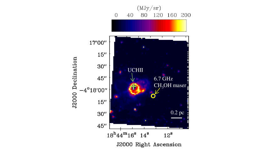
Figure 1: Spitzer’s IRAC 3.6 $\mu$m image toward G28.28$-$0.36. The open circle and cross indicate the 6.7 GHz methanol maser (Cyganowski et al., 2009) and ultracompact H II (UCH II) region (Urquhart et al., 2009), respectively.

In this paper, we carried out interferometric observations of cyanopolyynes (HC₃N, HC₅N, and HC₇N) toward the G28.28$-$0.36 high-mass star-forming region ($d=3$ kpc) with the Karl G. Jansky Very Large Array (VLA). Figure 1 shows the Spitzer IRAC 3.6 $\mu$m image toward the region. G28.28$-$0.36 is classified as an Extended Green Object (EGO) source (Cyganowski et al., 2008) from the Spitzer Galactic Legacy Infrared Mid-Plane Survey Extraordinaire (GLIMPSE; Benjamin et al., 2003). In Figure 1, the open circle and cross indicate the 6.7 GHz methanol maser (Cyganowski et al., 2009) and ultracompact H II (UCH II) region (Urquhart et al., 2009), respectively. The 6.7 GHz maser is considered to give us the exact position of MYSOs (Urquhart et al., 2013). A UCH II region seems to heat the environment. As shown in Figure 1, the ring structure around the UCH II region is suggestive of expanding motion and on-going massive star formation. We describe the observational details and data analyses in Section 2. The resultant images and spectra of cyanopolyynes are presented in Section 3. We compare the spatial distributions of cyanopolyynes with the infrared images and discuss possible formation mechanisms in Section 4.

2 Observations

The observations of G28.28$-$0.36 using the VLA Ka-band receiver were carried out in the C configuration with the 27 $\times$ 25-m antennas on March 20th, 2016 (Proposal ID = 16A-084, PI; Kotomi Taniguchi). The field of view (FoV) is $\sim$ 60$\farcs$4. Four spectral windows of the correlator were set at our target lines summarized in Table 1. All of these target lines were simultaneously observed. The channel separation of the correlator is 0.5 km s^-1. The angular resolutions and Position Angles (PA) for each line are summarized in Table 1.

The phase reference center was set at ($\alpha_{2000}$, $\delta_{2000}$) = (18^h44^m13$\fs$3, -04°18′03$\farcs$0), the 6.7 GHz methanol maser position. The pointing source is J1832$-$1035 at ($\alpha_{2000}$, $\delta_{2000}$) = (18^h32^m20$\fs$836, $-$10°35′11$\farcs$2). The absolute flux density calibration and the bandpass calibration were conducted by observing 3C286 at ($\alpha_{2000}$, $\delta_{2000}$) = (13^h31^m08$\fs$28798, +30°30′32$\farcs$9589). The gain/phase calibration was conducted by observing J1851+0035 at ($\alpha_{2000}$, $\delta_{2000}$) = (18^h51^m46$\fs$7217, +00°35′32$\farcs$414).

Table 1: Summary of target lines

Species	Transition	Rest Frequency	$E_{\rm{u}}/k$	Angular	PA
		(GHz)	(K)	Resolution	(deg)
HC3N	$J=4-3$	36.39232	4.4	0$\farcs$84 $\times$ 0$\farcs$63	-9.92
HC5N	$J=14-13$	37.276994	13.4	0$\farcs$81 $\times$ 0$\farcs$63	-11.04
HC7N	$J=33-32$	37.22349	30.4	0$\farcs$82 $\times$ 0$\farcs$63	-10.20
CH3CN	$J_{\rm K}=2_{0}-1_{0}$	36.7954747	2.6	0$\farcs$83 $\times$ 0$\farcs$64	-11.22

Note. — Rest frequencies are taken from the Cologne Database for Molecular Spectroscopy (CDMS; M$\ddot{\rm u}$ller et al., 2005) and the Jet Propulsion Laboratory catalog (JPL catalog; Pickett et al., 1998).

We conducted data reduction using the Common Astronomy Software Application (CASA; McMullin et al., 2007). We used the VLA calibration pipeline provided by the National Radio Astronomical Observatory (NRAO) to perform basic flagging and calibration.

The data cubes were imaged using the CLEAN task. Natural weighting was applied. The pixel size and image size are $0.2\arcsec$ and $1000\times 1000$ pixels. After the CLEAN, we smoothed the cube using the “imsmooth” command, applying $1\arcsec\times 1\arcsec$ and the position angle of $0\arcdeg$ with the gaussian kernel. The spatial resolution of $1\arcsec$ of the resultant images corresponds to $\sim 0.015$ pc. The $1\sigma$ values are approximately 0.6, 0.7, 0.7, and 0.6 mK for HC₃N, HC₅N, HC₇N, and CH₃CN, respectively. We made the moment zero images of HC₃N and HC₅N using the “immoments” task in CASA.

3 Results

Figure 2 shows the moment zero images of (a) HC₃N and (b) HC₅N in G28.28$-$0.36. The velocity components in the range $V_{\rm{LSR}}=47.5-51.5$ km s^-1 were integrated in these moment zero images. The spatial distribution of HC₃N is more extended than that of HC₅N, because of their excitation energies of the observed lines (Table 1). The observed HC₃N line has lower excitation energy ($E_{\rm{u}}/k=4.4$ K) than that of HC₅N ($E_{\rm{u}}/k=13.4$ K), and colder envelopes could be traced by HC₃N.

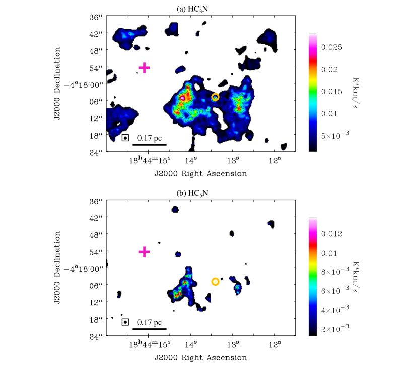
Figure 2: Moment zero images of (a) HC₃N and (b) HC₅N obtained with the VLA, including the data above $2\sigma$. The contour levels are 0.2, 0.4, 0.6, and 0.8 of their peak levels, where the peak intensities are 27.9 and 13.5 (mK $\cdot$ km s^-1) for (a) HC₃N and (b) HC₅N, respectively. The rms noise levels are 1.8 and 1.3 (mK $\cdot$ km s^-1) in the images of HC₃N and HC₅N, respectively. The orange open circle and magenta cross indicate the 6.7 GHz methanol maser (Cyganowski et al., 2009) and UCH II region (Urquhart et al., 2009), respectively. The filled circles at the bottom left corner represent the angular resolution of these images (1″).

Regarding HC₇N, the signal-to-noise ratio is low, which precludes determination of its spatial distribution. The bottom panel of Figure 3 shows HC₇N spectra, as well as HC₃N and HC₅N spectra, observed toward its four peak positions A$-$D indicated in the panel (b) of Figure 4. In order to improve the signal-to-noise ratio, we applied the $1\arcsec$ uvtaper for HC₇N data. The intensities of these spectra are estimated within $1.5\arcsec$ regions, which corresponds to the spatial resolution of HC₇N with the uvtaper. HC₇N is detected around the regions where HC₅N is detected as shown in the panel (b) of Figure 2.

CH₃CN emission is undetected at the rms noise level of 0.6 mK.

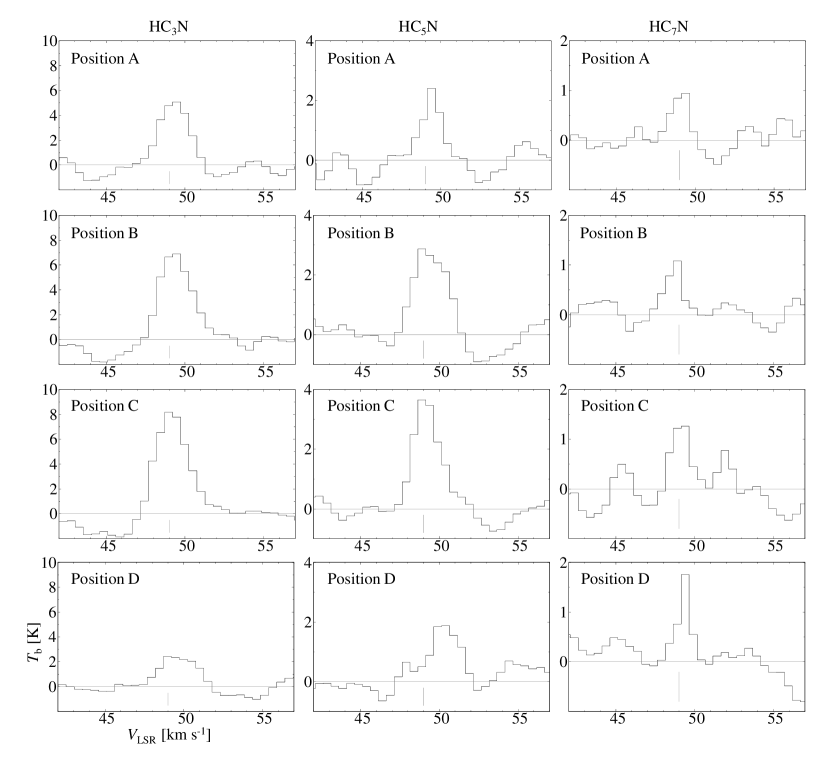
Figure 3: HC₃N, HC₅N, and HC₇N spectra at four HC₇N peak positions labeled as A$-$D, denoting in the panel (b) of Figure 4. The gray vertical lines show the systemic velocity of the G28.28-0.36 MYSO (49 km s^-1). The rms noise levels are 0.16, 0.20, and 0.12 K for HC₃N, HC₅N, and HC₇N spectra, respectively.

4 Discussion

4.1 Comparisons of Cyanopolyyne Ratios

We derived the column densities of HC₃N, HC₅N, and HC₇N at Position A (Figure 3) assuming the local thermodynamic equilibrium (LTE). We use the following formulae (Goldsmith & Langer, 1999):

$$\tau=-{\mathrm{ln}}\left[1-\frac{T_{\rm b}}{\left\{J(T_{\rm{ex}})-J(T_{\rm{bg}})\right\}}\right],$$ (1)

where

$$J(T)=\frac{h\nu}{k}\Bigl{\{}\exp\Bigl{(}\frac{h\nu}{kT}\Bigr{)}-1\Bigr{\}}^{-1},$$ (2)

and

$$N=\tau\frac{3h\Delta v}{8\pi^{3}}\sqrt{\frac{\pi}{4\mathrm{ln}2}}Q\frac{1}{\mu^{2}}\frac{1}{J_{\rm{lower}}+1}\exp\Bigl{(}\frac{E_{\rm{lower}}}{kT_{\rm{ex}}}\Bigr{)}\Bigl{\{}1-\exp\Bigl{(}-\frac{h\nu}{kT_{\rm{ex}}}\Bigr{)}\Bigr{\}}^{-1}.$$ (3)

In Equation (1), $\tau$ and $T_{\rm b}$ denote the optical depth and brightness temperature, respectively. $T_{\rm{ex}}$ and $T_{\rm{bg}}$ are the excitation temperature and the cosmic microwave background temperature ($\simeq 2.73$ K), respectively. $J$($T$) in Equation (2) is the effective temperature equivalent to that in the Rayleigh-Jeans law. In Equation (3), N, $\Delta v$, $Q$, $\mu$, and $E_{\rm{lower}}$ denote the column density, line width (FWHM), partition function, permanent electric dipole moment, and energy of the lower rotational energy level, respectively. The brightness temperatures and line widths are obtained by the gaussian fitting of spectra. Figure 7 in Appendix A shows the fitting results for each spectra, and the obtained spectral line parameters and permanent electric dipole moments of each species are summarized in Table 4.

We derived the column densities assuming the excitation temperatures of 15, 20, 30, and 50 K, respectively. The column densities of cyanopolyynes and the HC₃N : HC₅N : HC₇N ratios at each excitation temperature are summarized in Table 2. The uncertainties in the excitation temperatures do not significantly affect the derived column densities of HC₅N and HC₇N, and their derived column densities agree with each other within their the standard deviation errors. On the other hand, the uncertainties in the excitation temperatures bring larger differences in the HC₃N column density.

Table 2: Column densities of cyanopolyynes at Position A

$T_{\rm{ex}}$	$N$(HC3N)	$N$(HC5N)	$N$(HC7N)	HC3N : HC5N : HC7N
(K)	($\times 10^{14}$ cm-2)	($\times 10^{13}$ cm-2)	($\times 10^{13}$ cm-2)
15	$1.36\pm 0.14$	$4.4\pm 0.9$	$4.0\pm 1.2$	1.00 : 0.32 : 0.29
20	$1.47\pm 0.15$	$4.3\pm 0.9$	$3.1\pm 0.9$	1.00 : 0.29 : 0.21
30	$1.84\pm 0.19$	$4.9\pm 1.1$	$2.6\pm 0.8$	1.00 : 0.26 : 0.14
50	$2.7\pm 0.3$	$6.5\pm 1.4$	$2.8\pm 0.8$	1.00 : 0.24 : 0.11

Note. — The errors represent the standard deviation. The errors of column densities are derived from uncertainties of the gaussian fitting (see Table 4 in Appendix).

The HC₃N : HC₅N : HC₇N ratios at Position A are derived to be 1.0 : $\sim 0.3$ : $\sim 0.2$. The ratios in L1527, which is one of the WCCC sources, are 1.0 : $0.3-0.6$ : $\sim 0.1$ (Sakai et al., 2008, 2009). The tendency of the ratios at Position A seems to be similar to that in L1527.

4.2 Comparison of Spatial Distributions between Cyanopolyynes and 450 $\mu$m Dust Continuum

Figure 4 shows 450 $\mu$m dust continuum images overlaid by the black contours of moment zero images of (a) HC₃N and (b) HC₅N, respectively. The 450 $\mu$m data, which are available from the James Clerk Maxwell Telescope (JCMT) Science Archive, were obtained with the SCUBA installed on the JCMT. The main beam size of the SCUBA is $7.9\arcsec$ at 450 $\mu$m, corresponding to $\sim 0.11$ pc.

Three strong 450 $\mu$m continuum emission peaks can be recognized; the UCH II position, the north-west position from the UCH II, and the east position from the 6.7 GHz methanol maser. The spatial distribution of HC₅N is consistent with the 450 $\mu$m continuum peak of the east position from the 6.7 GHz methanol maser (hereafter Cyanopolyyne-rich clump, panel (b) of Figure 4). The spatial distribution of HC₃N seems to surround the Cyanopolyyne-rich clump (panel (a) of Figure 4), not only at the Cyanopolyyne-rich clump. HC₃N emission is also located at the west position of the 6.7 GHz methanol maser position, or the edge of the 450 $\mu$m continuum. Small HC₅N emission region is seen at the same edge of the 450 $\mu$m continuum. We will briefly discuss a possible origin of this emission region in Section 4.3.

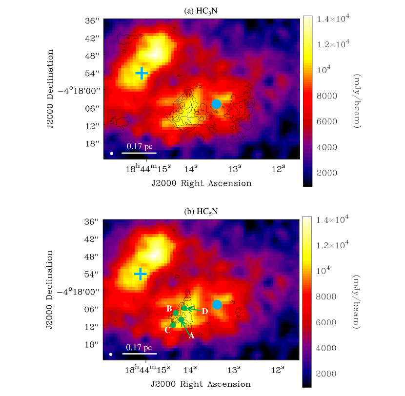
Figure 4: 450 $\mu$m continuum image obtained with the SCUBA installed on the JCMT overlaid by black contours of (a) HC₃N and (b) HC₅N moment zero images, the same ones as in Figure 2. The contour levels are 0.2, 0.4, 0.6, and 0.8 of their peak intensities 27.9 and 13.5 (mK $\cdot$ km s^-1) for (a) HC₃N and (b) HC₅N, respectively. The blue filled circle and blue cross indicate the 6.7 GHz methanol maser and UCH II region, respectively. The A–D positions are indicated as the green filled circles. The filed white circles at the bottom left corner represent the angular resolution of the images of HC₃N and HC₅N (1″).

4.3 Possible Nature of the 450 $\mu$m Continuum Peak Position associated with Cyanopolyynes

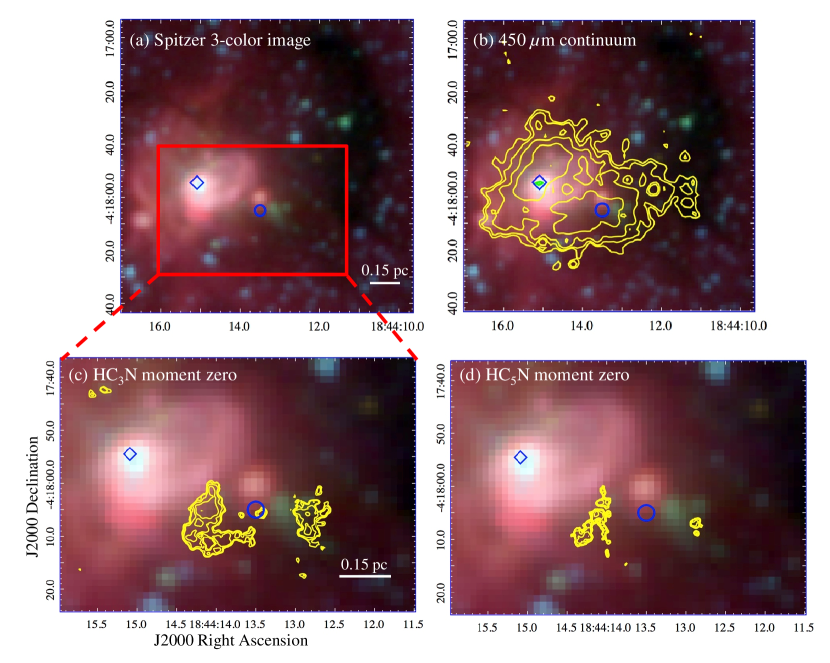
Figure 5: (a) Spitzer 3-color image (red; 8.0 $\mu$m, green; 4.5 $\mu$m, blue; 3.6 $\mu$m), overlaid by yellow contours showing (b) 450 $\mu$m continuum, (c) HC₃N moment zero image, and (d) HC₅N moment zero image. The green contour in panel (b) is the 8.3 mm continuum emission obtained with the VLA. The contour levels are 90, 80, 70, 60, 50 % of their peak levels. The blue open circle and diamond indicate the 6.7 GHz methanol maser and UCH II region, respectively.

We examine four possible types of objects of the Cyanopolyyne-rich clump (Section 4.2); a hot core, a starless clump, low- or intermediate-mass protostellar core(s), and a photo-dominated region (PDR) driven by the associated UCH II region.

Figure 5 shows the Spitzer 3-color (3.6 $\mu$m, 4.5 $\mu$m, 8.0 $\mu$m) images, overlaid by yellow contours showing (b) 450 $\mu$m continuum, (c) HC₃N moment zero image, and (d) HC₅N moment zero image, respectively. In panel (b), the green contours show the 8.3 mm continuum emission obtained simultaneously with cyanopolyynes by the VLA. The 8.3 mm continuum peak is compact and well consistent with the UCH II region. At the Cyanopolyyne-rich clump, no point source can be recognized from the Spitzer image, which suggests that no massive young protostar is currently present at the clump position. Therefore, the possibility of hot core is unrealistic.

We derived the average column density of H₂, $N$(H₂), of the Cyanopolyyne-rich clump from the 450 $\mu$m continuum data using the following formula (Shirley et al., 2005):

$$N({\rm{H}}_{2})=2.02\times 10^{20}{\rm{cm}}^{-2}\Bigl{(}e^{1.439(\lambda/{\rm{mm}})^{-1}(T/10{\rm{K}})^{-1}}-1\Bigr{)}\Bigl{(}\frac{\kappa_{\nu}}{0.01\>{\rm{cm}}^{2}\>{\rm{g}}^{-1}}\Bigr{)}^{-1}\Bigl{(}\frac{S_{\nu}^{\rm{beam}}}{{\rm{mJy}}\>{\rm{beam}}^{-1}}\Bigr{)}\Bigl{(}\frac{\theta_{\rm{HPBW}}}{10\>{\rm{arcsec}}}\Bigr{)}^{-2}\Bigl{(}\frac{\lambda}{{\rm{mm}}}\Bigr{)}^{3}.$$ (4)

We estimated the continuum flux ($S_{\nu}^{\rm{beam}}$) toward the Cyanopolyyne-rich clump within a size of $14\arcsec$, and the flux intensity is $9.7\times 10^{3}$ mJy beam^-1. We assumed that $\kappa_{\nu}$ is 0.0619 cm² g^-1 at $\lambda=450$ $\mu$m. $T$ is the dust temperature, and we assumed it to be $30\pm 15$ K. The derived $N$(H₂) value is ($2.8^{+8.1}_{-1.3}$)$\times 10^{22}$ cm^-2, which is similar to the typical value of massive clumps forming young star clusters (e.g., Shimoikura et al., 2018). The value is an average for the clump and then it can be considered as the lower limits for cores. The derived $N$(H₂) value for the Cyanopolyyne-rich clump is higher than the threshold value for star formation cores, $N$(H₂) $\approx 9\times 10^{21}$ cm^-2 (e.g., Tachihara et al., 2002). Hence, the Cyanopolyyne-rich clump is considered to contain deeply embedded low- or intermediate-mass protostellar core(s), and is not a starless clump.

In case that a low- or intermediate-mass protostar has been born, the WCCC mechanism is likely to work; cyanopolyynes are formed from CH₄ evaporated from grain mantles in the lukewarm gas ($T=20-30$ K). This may be supported by similar HC₃N : HC₅N : HC₇N ratios between this clump and L1527 (Section 4.1).

In order to investigate the possibility of the PDR, we compare the fractional abundances of cyanopolyynes at the Cyanopolyyne-rich clump with those derived from a PDR chemical network simulation (Le Gal et al., 2017). We derived the fractional abundances, $X$($a$)$=N$($a$)$/N$(H₂), of cyanopolyynes at Position A as summarized in Table 3. Recent chemical network simulation about the Horsehead nebula, which is one of the most studied PDRs, estimated the HC₃N and HC₅N abundances (Le Gal et al., 2017). The PDR and Core positions are positions with a visual extinctions ($A_{v}$) of $\sim 2$ mag and $\sim 10-20$ mag, respectively. We summarize the fractional abundances of these two positions in Table 3. The $X$(HC₃N) and $X$(HC₅N) values at the Cyanopolyyne-rich clump are significantly higher than those in PDR position by three order of magnitudes and more than four order of magnitudes, respectively. Moreover, the HC₃N and HC₅N fractional abundances at the Cyanopolyyne-rich clump are still higher than those in Core position in the PDR model by a factor of $\sim 55$ and $\sim 80$, respectively. Therefore, cyanopolyynes at the Cyanopolyyne-rich clump in the G28.28$-$0.36 high-mass star-forming region are not formed by the PDR chemistry. If we take large uncertainties in deriving $N$(H₂) values into consideration, the differences between the Cyanopolyyne-rich clump and the PDR models are plausible. However, we cannot completely exclude any effects from the UCHII region such as UV radiation.

Table 3: Comparison of fractional abundances of cyanopolyynes

Source	Method	$X$(HC3N)	$X$(HC5N)	$X$(HC7N)	Reference
		($\times 10^{-9}$)	($\times 10^{-9}$)	($\times 10^{-9}$)
Cyanopolyyne-rich clump	Observation	$6.6^{+5.5}_{-4.9}$	$1.7^{+1.5}_{-1.3}$	$0.9^{+0.8}_{-0.7}$	1
Horsehead nebula (PDR position)	Simulation	$3.1\times 10^{-3}$	$4.3\times 10^{-5}$	…	2
Horsehead nebula (Core position)	Simulation	0.12	0.022	…	2
L1527 (WCCC)	Observation	0.43 – 0.96	0.05 – 0.24	$\sim 0.05$	3,4,5

Note. — The errors represent the standard deviation.

We also compare the fractional abundances of HC₃N, HC₅N, and HC₇N at the Cyanopolyyne-rich clump to those in L1527. These fractional abundances at the Cyanopolyyne-rich clump are higher than those in L1527 by a factor of $7-15$, $7-37$, and $\sim 17$, respectively. Hence, the cyanopolyynes at the Cyanopolyyne-rich clump seem to be more abundant compared to L1527, even if we take uncertainties in fractional abundances into account. It cannot be excluded that several low-mass protostars are concentrated within a small region (e.g., $\sim 0.02$ pc corresponding to $1.5\arcsec$ at the distance of 3 kpc). As another interpretation, these results may imply that there is an intermediate-mass protostar because an intermediate-mass protostar heats its wider surroundings compared to a low-mass protostar; the size of lukewarm envelopes will be larger and the column densities of carbon-chain species in such lukewarm envelopes will increase. This could explain the results that the cyanopolyynes at the Cyanopolyyne-rich clump are more abundant than those in L1527.

In Figure 5 (d), compact HC₅N emission region is located at the west position of the 6.7 GHz methanol maser position. This position corresponds to the edge of the 4.5 $\mu$m emission, which seems to trace shock regions (Cyganowski et al., 2008). Figure 6 shows spectra of HC₃N and HC₅N at the shock region. The line widths (FWHM) derived from the Gaussian fit are $2.7\pm 0.2$ and $2.6\pm 0.2$ km s^-1 for HC₃N and HC₅N, respectively. These line widths at the shock region are wider those at the Cyanopolyyne-rich clump, $2.05\pm 0.16$ and $1.4\pm 0.2$ km s^-1 for HC₃N and HC₅N, respectively. These results probably support that the cyanopolyynes are the shock origin. Molecules evaporated from grain mantles such as C₂H₂ may be parent species of the cyanopolyynes. It is still unclear whether HC₅N is formed and can survive in shock regions, but this may be the first observational result showing that HC₅N can be enhanced in shock regions.

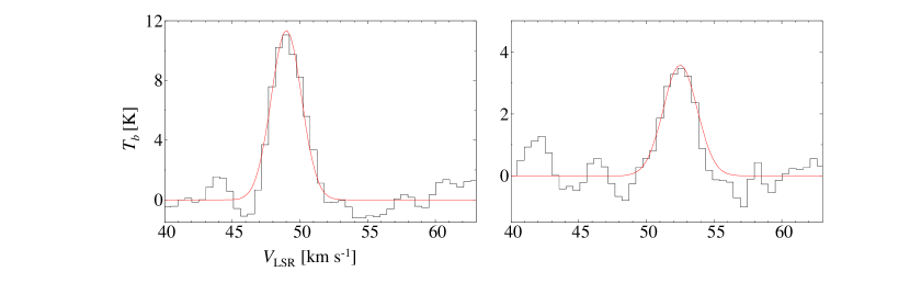
Figure 6: Spectra of HC₃N and HC₅N at the shock region. The red lines show the Gaussian fitting results.

4.4 Comparison with Previous Single-Dish Telescope Observations

Taniguchi et al. (2017) reported the detection of high-excitation-energy ($E_{\rm{u}}/k\simeq 100$ K) lines of HC₅N with the Nobeyama 45-m radio telescope (HPBW = 18″) toward the methanol maser position, which is considered to be a MYSO position (Urquhart et al., 2013). The significant HC₅N peak is not seen at the methanol maser position in the VLA map. This is probably caused by the different excitation energies of the observed lines. The lines observed with the VLA have low excitation energies (Table 1), and preferably trace lower-temperature regions such as low- or intermediate-mass protostellar cores or envelopes. On the other hand, HC₅N emission observed with the Nobeyama 45-m telescope seems to come from higher-temperature regions closer to the methanol maser or the MYSO. In these higher-temperature regions, HC₅N should be highly excited and low excitation energy lines observed with the VLA should be weak. In contrast, the hotter components detected with the Nobeyama 45-m telescope were not detected with the VLA, because the low-excitation-energy lines are not suitable tracers of the hot components. Combining with the VLA and Nobeyama 45-m telescope results, both the MYSO associated with the methanol maser and low- or intermediate-mass protostellar core(s) at the Cyanopolyyne-rich clump appear to be rich in cyanopolyynes.

It is still unclear why the G28.28$-$0.36 high-mass star-forming region is a cyanopolyyne-rich/COMs-poor source (Taniguchi et al., 2018). Studies about chemical diversity among high-mass star-forming regions will become a key to our understanding of massive star formation processes. We need the high-spatial-resolution and higher-frequency band observations in order to investigate the spatial resolution of higher temperature components of cyanopolyynes to confirm that cyanopolyynes exist at the hot core position.

5 Conclusions

We have carried out interferometric observations of cyanopolyynes (HC₃N, HC₅N, and HC₇N) toward the G28.28$-$0.36 high-mass star-forming region with the VLA Ka-band. We obtained the moment zero images of HC₃N and HC₅N and tentatively detected HC₇N. The spatial distributions of HC₃N and HC₅N are consistent with the 450 $\mu$m dust continuum clump, i.e., the Cyanopolyyne-rich clump. The HC₃N : HC₅N : HC₇N column density ratios are estimated at 1.0 : $\sim 0.3$ : $\sim 0.2$ at Position A. The Cyanopolyyne-rich clump seems to contain deeply embedded low- or intermediate-mass protostellar core(s). The most probable formation mechanism of the cyanopolyynes at the Cyanopolyyne-rich clump is the WCCC mechanism. We possibly found the HC₃N and HC₅N emission in the shock region.

Appendix A Gaussian Fitting Results and Spectral Line Parameters

We show the gaussian fitting results for the spectra of HC₃N, HC₅N, and HC₇N at Position A in Figure 7. The obtained spectral line parameters are summarized in Table 4.

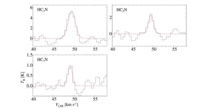
Figure 7: Spectra of HC₃N, HC₅N, and HC₇N at Position A obtained with the VLA. The best gaussian fits are shown overlaid in red.

Table 4: Spectral line parameters at Position A

Species	$\mu$	$T_{\rm{b}}$	FWHM	$\int T_{\mathrm{b}}dv$
	(Debye)	(K)	(km s-1)	(K km s-1)
HC3N	3.73	$5.4\pm 0.4$	$2.05\pm 0.16$	$11.7\pm 1.2$
HC5N	4.33	$2.3\pm 0.3$	$1.4\pm 0.2$	$3.5\pm 0.8$
HC7N	4.82	$1.0\pm 0.2$	$1.3\pm 0.3$	$1.3\pm 0.4$

Note. — The errors represent the standard deviation. Values of their permanent electric dipole moments are taken from the Cologne Database for Molecular Spectroscopy (CDMS; M$\ddot{\rm u}$ller et al., 2005).

References

- Bachiller & Pérez Gutiérrez (1997) Bachiller, R., & Pérez Gutiérrez, M. 1997, ApJ, 487, L93
- Belloche et al. (2013) Belloche, A., Müller, H. S. P., Menten, K. M., Schilke, P., & Comito, C. 2013, A&A, 559, A47
- Benjamin et al. (2003) Benjamin, R. A., Churchwell, E., Babler, B. L., et al. 2003, PASP, 115, 953
- Bergner et al. (2018) Bergner, J. B., Guzmán, V. G., Öberg, K. I., Loomis, R. A., & Pegues, J. 2018, ApJ, 857, 69
- Calcutt et al. (2018) Calcutt, H., Jørgensen, J. K., Müller, H. S. P., et al. 2018, arXiv:1804.09210
- Chapman et al. (2009) Chapman, J. F., Millar, T. J., Wardle, M., Burton, M. G., & Walsh, A. J. 2009, MNRAS, 394, 221
- Cyganowski et al. (2009) Cyganowski, C. J., Brogan, C. L., Hunter, T. R., & Churchwell, E. 2009, ApJ, 702, 1615
- Cyganowski et al. (2008) Cyganowski, C. J., Whitney, B. A., Holden, E., et al. 2008, AJ, 136, 2391-2412
- Esplugues et al. (2013) Esplugues, G. B., Cernicharo, J., Viti, S., et al. 2013, A&A, 559, A51
- Feng et al. (2015) Feng, S., Beuther, H., Henning, T., et al. 2015, A&A, 581, A71
- Fontani et al. (2017) Fontani, F., Ceccarelli, C., Favre, C., et al. 2017, A&A, 605, A57
- Goldsmith & Langer (1999) Goldsmith, P. F., & Langer, W. D. 1999, ApJ, 517, 209
- Green et al. (2014) Green, C.-E., Green, J. A., Burton, M. G., et al. 2014, MNRAS, 443, 2252
- Hassel et al. (2008) Hassel, G. E., Herbst, E., & Garrod, R. T. 2008, ApJ, 681, 1385
- Hirota et al. (2009) Hirota, T., Ohishi, M., & Yamamoto, S. 2009, ApJ, 699, 585
- Jaber Al-Edhari et al. (2017) Jaber Al-Edhari, A., Ceccarelli, C., Kahane, C., et al. 2017, A&A, 597, A40
- Jørgensen et al. (2002) Jørgensen, J. K., Schöier, F. L., & van Dishoeck, E. F. 2002, A&A, 389, 908
- Lee et al. (2015) Lee, K. I., Dunham, M. M., Myers, P. C., et al. 2015, ApJ, 814, 114
- Le Gal et al. (2017) Le Gal, R., Herbst, E., Dufour, G., et al. 2017, A&A, 605, A88
- McMullin et al. (2007) McMullin, J. P., Waters, B., Schiebel, D., Young, W., & Golap, K. 2007, Astronomical Data Analysis Software and Systems XVI, 376, 127
- Mller et al. (2005) Mller, H. S. P., Schlder, F., Stutzki, J., & Winnewisser, G. 2005, JMoSt, 742, 215
- Mumma & Charnley (2011) Mumma, M. J., & Charnley, S. B. 2011, ARA&A, 49, 471
- Öberg et al. (2015) Öberg, K. I., Guzmán, V. V., Furuya, K., et al. 2015, Nature, 520, 198
- Pickett et al. (1998) Pickett, H. M., Poynter, R. L., Cohen, E. A., et al. 1998, J. Quant. Spec. Radiat. Transf., 60, 883
- Sakai et al. (2008) Sakai, N., Sakai, T., Hirota, T., & Yamamoto, S. 2008, ApJ, 672, 371
- Sakai et al. (2009) Sakai, N., Sakai, T., Hirota, T., & Yamamoto, S. 2009, ApJ, 702, 1025
- Sakai & Yamamoto (2013) Sakai, N., & Yamamoto, S. 2013, Chemical Reviews, 113, 8981
- Sanhueza et al. (2012) Sanhueza, P., Jackson, J. M., Foster, J. B., et al. 2012, ApJ, 756, 60
- Shimoikura et al. (2018) Shimoikura, T., Dobashi, K., Nakamura, F., Matsumoto, T., & Hirota, T. 2018, ApJ, 855, 45
- Shirley et al. (2005) Shirley, Y. L., Nordhaus, M. K., Grcevich, J. M., et al. 2005, ApJ, 632, 982
- Suzuki et al. (1992) Suzuki, H., Yamamoto, S., Ohishi, M., et al. 1992, ApJ, 392, 551
- Tachihara et al. (2002) Tachihara, K., Onishi, T., Mizuno, A., & Fukui, Y. 2002, A&A, 385, 909
- Taniguchi et al. (2017) Taniguchi, K., Saito, M., Hirota, T., et al. 2017, ApJ, 844, 68
- Taniguchi et al. (2018) Taniguchi, K., Saito, M., Majumdar, L., et al. 2018a, arXiv:1804.05205
- Taniguchi et al. (2016) Taniguchi, K., Saito, M., & Ozeki, H. 2016, ApJ, 830, 106
- Urquhart et al. (2009) Urquhart, J. S., Hoare, M. G., Purcell, C. R., et al. 2009, A&A, 501, 539
- Urquhart et al. (2013) Urquhart, J. S., Moore, T. J. T., Schuller, F., et al. 2013, MNRAS, 431, 1752