Statistical State Dynamics Based Study of the Role of Nonlinearity in the Maintenance of Turbulence in Couette Flow

Abstract

While linear non-normality underlies the mechanism of energy transfer from the externally driven flow to the perturbation field that sustains turbulence, nonlinearity is also known to play an essential role. The goal of this study is to better understand the role of nonlinearity in sustaining turbulence. The method used in this study is implementation in Couette flow of a statistical state dynamics (SSD) closure at second order in a cumulant expansion of the Navier-Stokes equations in which the averaging operator is the streamwise mean. The perturbations in this SSD are the deviations from the streamwise mean and two mechanisms potentially contributing to maintaining these second cumulant perturbations are identified. These are parametric perturbation growth arising from interaction of the perturbations with the fluctuating mean flow and transient growth of perturbations arising from nonlinear interaction between components of the perturbation field. By the method of comparing the turbulence maintained in the SSD and in the associated direct numerical simulation (DNS) in which these mechanisms have been selectively included and excluded, parametric growth is found to maintain the perturbation field of the turbulence while the more commonly invoked mechanism associated with transient growth of perturbations arising from scattering by nonlinear interaction is found to suppress perturbation growth. In addition to verifying that the parametric mechanism maintains the perturbations in DNS it is also verified that the Lyapunov vectors are the structures that dominate the perturbation energy and energetics in DNS. It is further verified that these vectors are responsible for maintaining the roll circulation that underlies the self-sustaining process (SSP) and in particular the maintenance of the fluctuating streak that supports the parametric perturbation growth.

I Introduction

Turbulence is widely regarded as the primary exemplar of an essentially nonlinear phenomenon. However, the mechanism by which energy is transferred in shear flows from the externally forced component of the flow to the broad spectrum of spatially and temporally varying perturbations is through linear non-normal interaction between these components Boberg and Brosa (1988); Henningson and Reddy (1994); Farrell and Ioannou (1994); Kim and Lim (2000); Farrell and Ioannou (2012). Nevertheless, nonlinearity participates in an essential way in the cooperative interaction between the mean and the perturbation by which turbulence self-sustains. Our goal in this study is to provide a more comprehensive understanding of the role of nonlinearity and its interaction with linear non-normality in the maintenance of turbulence.

Because realistic wall-turbulence is maintained by the statistical state dynamics (SSD) of the Navier-Stokes equations closed at second order with the averaging operator chosen to be the streamwise mean Farrell and Ioannou (2012); Farrell et al. (2017a); Farrell and Ioannou (2017) it is inviting to study the mechanism of wall-turbulence using this SSD which has the advantage of complete analytic characterization. We employ SSD-based analysis to examine the role of nonlinearity in turbulence maintenance, specifically its role in maintaining the perturbations from the streamwise mean at statistical equilibrium.

A commonly invoked physical process by which this maintenance of the perturbation field is hypothesized to occur is through recycling of perturbations which have completed their transient amplification into new perturbations that are at the initial stage of transient growth leading to renewed growth and in this way to turbulence maintenance Boberg and Brosa (1988); Trefethen et al. (1993); Gebhardt and Grossmann (1994); Baggett and Trefethen (1997); Grossmann (2000). This idea underlies the regeneration cycle which was inspired by observations in which streak breakdown produces perturbations configured to give rise to new streak formation Jiménez (1994). An alternative mechanism of perturbation maintenance that has been shown to support turbulence in the second order SSD of a variety of turbulent shear flows is a process of parametric growth in which fluctuation of the streamwise mean flow maintains the perturbation field Farrell and Ioannou (2012); Thomas et al. (2014); Farrell et al. (2017a, 2016); Farrell and Ioannou (2017).

It was shown previously that realistic turbulence is maintained by restricting the SSD dynamics to the second of these mechanisms; this was done by simply neglecting the perturbation-perturbation nonlinearity in the second order closure Farrell and Ioannou (2012); Thomas et al. (2015); Bretheim et al. (2015); Farrell et al. (2016). However, although these results establish that the perturbation-perturbation nonlinearity is not necessary for perturbations from the streamwise mean as well as the turbulence itself to be maintained in a second order closure, the influence of perturbation-perturbation nonlinearity on the turbulence is still of interest because it has been implicated in Navier-Stokes turbulence dynamics by interpretations of DNS data Jiménez (1994); Hamilton et al. (1995); Jiménez and Pinelli (1999); Kim and Lim (2000) and also in part because perturbation-perturbation nonlinearity alone has been shown to maintain turbulent state analogues in simple model systems Trefethen et al. (1993); Gebhardt and Grossmann (1994); Baggett and Trefethen (1997); Grossmann (2000). Given that the parametric mechanism supports realistic turbulence in the absence of perturbation-perturbation nonlinearity, the experiment available to us is to include the perturbation-perturbation nonlinearity and assess the influence of the addition of this term on the parametrically maintained turbulence.

The specific SSD model examined is a reduced non-linear model (RNL) in which the second cumulant is approximated as the state covariances obtained from the perturbation dynamics in which the nonlinearity has been neglected. We find by comparing RNL simulations made using this model with DNS that the turbulence and its energetics are similar whether the nonlinear interactions between perturbations from the streamwise mean are retained or neglected. This result demonstrates that the parametric mechanism dominates in the maintenance of the turbulence and in fact closer examination of the energetics reveals that the perturbation-perturbation nonlinearity rather than serving to support the turbulence actually decreases effectiveness of energy transfer from the mean to the perturbations. Furthermore, it is also verified that the parametrically maintained Lyapunov vectors analytically predicted to support the turbulence by RNL that dominate the perturbation energy and energetics in DNS. It is further verified that moreover these vectors are also found to be responsible for maintaining the roll circulation that underlies the self sustaining process (SSP) and in particular the maintenance of the fluctuating streak that supports the parametric perturbation growth.

II Formulation

In order to study the mechanism by which nonlinearity between streamwise varying components in a turbulent shear flow participate in the maintenance of turbulence we begin by partitioning the velocity field of plane parallel Couette flow into streamwise mean and perturbation components, or equivalently into the $k_{x}=0$ and the $k_{x}\neq 0$ components of the Fourier decomposition of the flow field, where $k_{x}$ is the wavenumber in the streamwise, $x$, direction. In this decomposition the flow field is partitioned as:

$$\mathbf{u}=\mathbf{U}(y,z,t)+\mathbf{u}^{\prime}(x,y,z,t)~{},$$ (1)

with cross-stream direction $y$ and spanwise direction $z$. It is important to note that in this decomposition the mean flow retains temporal variation in its spanwise structure and particularly that this mean flow includes the time-dependent streaks. The mean used in the cumulant expansion is fundamental to formulating an SSD that retains the physical mechanism of turbulence in shear flow. The centrality of spanwise variation of the mean flow, which is associated with the fluctuating streak component, to the maintenance of turbulence has been demonstrated by numerical experiments that show turbulence is not sustained when the streaks are sufficiently damped or removed Jiménez and Pinelli (1999). Given that in the SSD turbulent state spanwise and temporal inhomogeneity are required to allow the parametric instability of the fluctuating streamwise streak to be supported it is necessary to allow both spanwise and temporal variations in the mean operator used to define the cumulants in the SSD in (1).

The non-dimensional Navier-Stokes equations expressed using this mean and perturbation partition are:

$$\partial_{t}\mathbf{U}+\underbrace{\mathbf{U}\boldsymbol{\cdot}\boldsymbol{\nabla}\mathbf{U}}_{N_{1}}+\boldsymbol{\nabla}P-\Delta\mathbf{U}/R=\underbrace{-\langle\mathbf{u}^{\prime}\boldsymbol{\cdot}\boldsymbol{\nabla}\mathbf{u}^{\prime}\rangle_{x}}_{N_{2}}\ ,$$ (2a)

$$\partial_{t}\mathbf{u}^{\prime}+\underbrace{\mathbf{U}\boldsymbol{\cdot}\boldsymbol{\nabla}\mathbf{u}^{\prime}+\mathbf{u}^{\prime}\boldsymbol{\cdot}\boldsymbol{\nabla}\mathbf{U}}_{N_{3}}+\boldsymbol{\nabla}p^{\prime}-\Delta\mathbf{u}^{\prime}/R$$

$$=\underbrace{-\left(\mathbf{u}^{\prime}\boldsymbol{\cdot}\boldsymbol{\nabla}\mathbf{u}^{\prime}-\langle\mathbf{u}^{\prime}\boldsymbol{\cdot}\boldsymbol{\nabla}\mathbf{u}^{\prime}\rangle_{x}\,\right)}_{N_{4}}~{},$$ (2b)

$$\boldsymbol{\nabla}\boldsymbol{\cdot}\mathbf{U}=0\ ,\ \ \ \boldsymbol{\nabla}\boldsymbol{\cdot}\mathbf{u}^{\prime}=0\ ,$$ (2c)

where $R=U_{w}h/\nu$ is the Reynolds number and $\pm U_{w}$ the wall velocity at $y=\pm h$. The flow satisfies no-slip boundary conditions in the cross-stream direction: $\mathbf{U}(x,\pm h,z,t)=(\pm U_{w},0,0)$, $\mathbf{u}^{\prime}(x,\pm h,z,t)=(0,0,0)$ and periodic boundary conditions in the $z$ and $x$ directions. Lengths are nondimensionalized by $h$, velocities by $U_{w}$, and time by $h/U_{w}$. Averaging is denoted with angle brackets $\langle\boldsymbol{\cdot}\rangle$ with the bracket subscript indicating the averaging variable, so that e.g. the streamwise mean velocity is $\mathbf{U}\stackrel{{\scriptstyle\mathrm{def}}}{{=}}\langle\mathbf{u}\rangle_{x}=L_{x}^{-1}\int_{0}^{L_{x}}\mathbf{u}~{}dx$, where $L_{x}$ is the streamwise length of the channel. The Navier-Stokes equations with this decomposition are referred to as the DNS system. In (2) we have indicated with an underbrace the nonlinear terms in DNS of primary relevance to our study. In the streamwise mean flow equation (2a) nonlinear interactions among $k_{x}=0$ flow components are referred to as $N_{1}$ and Reynolds stress divergence term produced by nonlinear interaction between the $k_{x}$ and $-k_{x}$ flow components with $k_{x}\neq 0$, is referred to as $N_{2}$. In the perturbation equation (2b) the interaction between the instantaneous streamwise mean flow and the $k_{x}\neq 0$ flow components is referred to as $N_{3}$. If the mean flow $\mathbf{U}$ is a solution of (2), interaction $N_{3}$ between the perturbations and this mean flow $\mathbf{U}$ can be viewed in the perturbation equation (2b) as a linear interaction. From that perspective, in the perturbation equation  (2b) transfer of energy from the mean to the perturbations is due to linear non-normal interaction between $\mathbf{U}$ and the perturbations, $\mathbf{u}^{\prime}$, although from the perspective of the DNS system (2) as a whole this term is nonlinear. This is a crucial point in the analysis to follow as we will be taking $\mathbf{U}$ in $N_{3}$ to be known and this term to be linear from the perspective of the perturbation equation (2b). Finally, the nonlinear interaction between perturbation components $k_{x_{1}}\neq 0$ and $k_{x_{2}}\neq 0$, with $k_{x_{1}}\neq-k_{x_{2}}$ is referred to as $N_{4}$.

Transition to and maintenance of a self-sustained turbulent state results even when only nonlinearity $N_{2}$ and term $N_{3}$ are retained Farrell and Ioannou (2012). By retaining both nonlinearities $N_{1}$ and $N_{2}$ and term $N_{3}$ we obtain the restricted non-linear system (RNL):

$$\partial_{t}\mathbf{U}+\mathbf{U}\boldsymbol{\cdot}\boldsymbol{\nabla}\mathbf{U}+\boldsymbol{\nabla}P-\Delta\mathbf{U}/R=-\langle\mathbf{u}^{\prime}\boldsymbol{\cdot}\boldsymbol{\nabla}\mathbf{u}^{\prime}\rangle_{x}\ ,$$ (3a)

$$\partial_{t}\mathbf{u}^{\prime}+\mathbf{U}\boldsymbol{\cdot}\boldsymbol{\nabla}\mathbf{u}^{\prime}+\mathbf{u}^{\prime}\boldsymbol{\cdot}\boldsymbol{\nabla}\mathbf{U}+\boldsymbol{\nabla}p^{\prime}-\Delta\mathbf{u}^{\prime}/R=0~{},$$ (3b)

$$\boldsymbol{\nabla}\boldsymbol{\cdot}\mathbf{U}=0\ ,\ \ \ \boldsymbol{\nabla}\boldsymbol{\cdot}\mathbf{u}^{\prime}=0\ .$$ (3c)

It has been confirmed that this RNL system supports a realistic self-sustaining process (SSP) which maintains a turbulent state in minimal channels Farrell and Ioannou (2012); Farrell et al. (2017b), in channels of moderate sizes at both low and high Reynolds numbers (at least for $R_{\tau}\leq 1000$) Thomas et al. (2014); Farrell et al. (2016, 2017a), and also in very long channels Thomas et al. (2015).

Consider in isolation the time varying mean flow $\mathbf{U}$ obtained from a state of turbulence either of the RNL or the DNS system. Sufficiently small perturbations, $\mathbf{u}^{\prime}$, to this mean flow evolve according to

$$\partial_{t}\mathbf{u}^{\prime}+\mathbf{U}\boldsymbol{\cdot}\boldsymbol{\nabla}\mathbf{u}^{\prime}+\mathbf{u}^{\prime}\boldsymbol{\cdot}\boldsymbol{\nabla}\mathbf{U}+\boldsymbol{\nabla}p^{\prime}-\Delta\mathbf{u}^{\prime}/R~{}=0~{},~{}~{}\boldsymbol{\nabla}\boldsymbol{\cdot}\mathbf{u}^{\prime}=0~{},$$ (4)

which is the perturbation equation (3b) of the RNL system, while in the DNS system the finite perturations $\mathbf{u}^{\prime}$ obey the different equation (2b) with the $N_{4}$ term included. In the self-sustained RNL turbulence the perturbations, $\mathbf{u}^{\prime}$, that evolve under the linear dynamics (3b) or equivalently under (4) remain finite and bounded. Therefore the mean-flow, $\mathbf{U}$, of the RNL turbulent state is stable in the sense that perturbations, i.e. the streamwise varying flow components, $\mathbf{u}^{\prime}$, that evolve under (4), have zero asymptotic growth rate and the mean flow can be considered to be in the critical state of neutrality, poised between stability and instability. A question that will be addressed in this paper is whether the mean flow, $\mathbf{U}$, that is obtained from a DNS shares this property of being adjusted similarly to neutrality in the sense that perturbations, $\mathbf{u}^{\prime}$, that evolve under (4), remain bounded and therefore have vanishing asymptotic growth rate and the mean flow of the DNS can therefore be considered to be similarly in a critical state of parametric neutrality when proper account is taken of dissipation. If the turbulent mean flow $\mathbf{U}$ of the DNS can be shown to be neutral, in this sense of parametric neutrality, and the associated perturbations can be shown to be the Lyapunov vectors of this $\mathbf{U}$, then the mechanism of turbulence identified analytically in the RNL system, in which the perturbations arise from parametric instability of the mean flow with the mean flow being regulated to neutrality through quasi-linear interaction with the perturbation field, will have been extended to DNS. Identification of DNS turbulence dynamics with that of RNL would represent a fundamental advance in understanding because RNL turbulence is fully and analytically characterized so that this identification would imply extension of the full analytical characterization of RNL turbulence to the DNS system. For this program to succeed it is required to show that the dynamically substantive difference between the RNL system and the DNS, which is the appearance in DNS of the perturbation-perturbation nonlinearity $N_{4}$, does not fundamentally change the dynamics of turbulence.

An illustrative aspect of the insight that can be gained by identifying in the DNS system the mechanisms that are known to be operating in the RNL system relates to the adjustment of turbulence to a statistically stationary state. The mechanism by which the statistical state of turbulence in the RNL system is regulated to its statistical mean can be related to an influential conjecture that in a turbulent system the linear instability of the mean state is adjusted by quasi-linear interaction with the perturbations to a state of modal neutrality Malkus (1956); Herring (1963); Stone (1978). The theory of turbulence based on the second order SSD we use has in common with this influential hypothesis the concept of adjustment by quasi-linear interaction between the mean flow and perturbations to neutrality as the general mechanism determining the statistical state of turbulence. While turbulent convection (Malkus, 1954; Malkus and Veronis, 1958) displays a usefully close approximate adherence to modal neutrality when both the spatial and temporal means are taken to define the mean flow, the turbulent mean state of wall-bounded shear flows, defined as the streamwise, spanwise and temporal mean, $\langle\mathbf{U}\rangle_{z,t}$, is hydrodynamically stable and far from neutrality in apparently strong violation of the adjustment to neutrality conjecture Reynolds and Tiederman (1967). However, study of RNL turbulence suggests that this program is essentially correct and can be extended to wall-turbulence requiring only the additional recognition that the instability to be equilibrated is the instability of the time-dependent operator associated with linearization about the temporally varying streamwise mean flow. Among the theoretical advances arising from identifying the mechanism of RNL turbulence and that of DNS is extension of this physical mechanism determining the statistical steady state to DNS turbulence.

The maximum growth rate of perturbations to the streamwise mean governed by the linear dynamics of (4) is given by the top Lyapunov exponent of $\mathbf{u}^{\prime}$ defined as:

$$\lambda_{Lyap}=\lim_{t\to\infty}\frac{\log|\mathbf{u}^{\prime}|}{t}~{}.$$ (5)

RNL turbulence with mean (1) satisfies the neutrality conjecture precisely under our interpretation because for RNL

$$\lambda_{Lyap}=0~{}.$$ (6)

An issue we wish to examine in this work is whether DNS turbulence (with the $N_{4}$ term included) is similarly neutral in the Lyapunov sense with its perturbations being supported by parametric growth on its fluctuating mean flow and with perturbation structure being that predicted by the associated Lyapunov vector structures. Specifically, whether fluctuations, $\mathbf{u}^{\prime}$, evolving under (4) on the time dependent mean flow, $\mathbf{U}$, that has been obtained from a turbulent DNS, have $\lambda_{Lyap}$, as defined in (5), zero when proper account is taken of dissipative processes and in addition whether the predicted Lyapunov structure can be verified to be maintaining the perturbations in the DNS. We caution the reader that the Lyapunov structures and exponents we are calculating are not the familiar Lyapunov structures and exponents associated with small perturbations to the full turbulent state trajectory. This more familiar use of Lyapunov exponents and associated vectors is concerned with growth of perturbations $\delta\mathbf{U}$, $\delta\mathbf{u}^{\prime}$ to the tangent linear dynamics of the full Navier-Stokes equations linearized about the entire turbulent trajectory $\mathbf{U}$, $\mathbf{u}^{\prime}$. This tangent linear dynamics typically has many positive Lyapunov exponents Keefe et al. (1992). We instead calculate the Lyapunov exponents and structures only of perturbations, $\mathbf{u}^{\prime}$, evolving under the linear dynamics (4) about the time dependent mean flow $\mathbf{U}$ and there are typically only a small set of these that correspond to the perturbation component of the turbulent state which are neutrally stable while the rest are damped. It is also important to recognize that the parametric perturbation evolution equation (4) governing the perturbation dynamics of RNL is not limited to small perturbation amplitude because the perturbation equation is strictly linear and the nonlinearity required to regulate the perturbations to their finite statistical equilibrium state is not explicit in (4) but rather is contained in the Reynolds stress feedback term $N_{2}$ appearing in the mean equation which serves to provide feedback regulation of the mean state to neutral Lyapunov stability.

The mean used in the cumulant expansion is fundamental to formulating an SSD that retains the physical mechanism of turbulence in shear flow. The centrality of spanwise variation of the mean flow, which is associated with the streak component, to the maintenance of turbulence has been demonstrated by numerical experiments that show turbulence is not sustained when the streaks are sufficiently damped or removed Jiménez and Pinelli (1999). Given that in the SSD turbulent state spanwise and temporal inhomogeneity are required to allow the parametric instability of the the fluctuating streamwise streak to be supported it is necessary to allow both spanwise and temporal variations in the mean operator used to define the cumulants in the SSD which requires representation (1). The requirement that the streamwise mean be taken to support turbulence in a second order SSD provides a partition of the mechanisms by which nonlinearity enters the dynamics. This naturally compelled partition is into the completely characterized nonlinearity mechanism of the RNL dynamics and the remaining nonlinearity that has not yet been completely characterized which is that contained in the $N_{4}$ term of the DNS system perturbation equation.

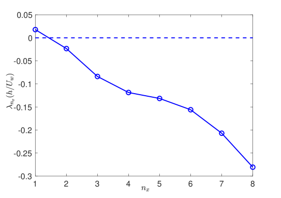
Figure 1: The top Lyapunov exponent of perturbations with channel wavenumbers $n_{x}=1,\dots,8$ evolving under the time-dependent turbulent mean flow in the DNS, $\mathbf{U}$. The Lyapunov exponent of all $n_{x}\geq 2$ components of $\mathbf{u}^{\prime}$ is negative. For comparison, the least stable mode of the streamwise-spanwise-temporal mean of $\mathbf{U}$ has decay rate $\sigma=-0.12~{}U_{w}/h$ at $n_{x}=1$ and $n_{z}=3$. The Lyapunov exponent was nondimensionalized using advective time units, $h/U_{w}$. A plane Couette channel at $R=600$ was used.

We now compare RNL and DNS dynamics in order to gain insight into the role of perturbation-perturbation nonlinearity $N_{4}$ in the maintenance and regulation of turbulence. The $N_{4}$ term in (2b) does not contribute directly to maintaining the perturbation energy because the perturbation-perturbation interactions redistribute energy internally among the streamwise $k_{x}\neq 0$ components of the flow and the term $\langle\mathbf{u}^{\prime}\boldsymbol{\cdot}N_{4}\rangle_{x,y,z}$ is zero  in the DNS. From (2b) we obtain that the perturbation energy density, $E_{p}=\langle|\mathbf{u}^{\prime}|^{2}/2\rangle_{x,y,z}$, evolves according to:

$$\frac{dE_{p}}{dt}=\underbrace{\left\langle\mathbf{u}^{\prime}\boldsymbol{\cdot}\left(-\mathbf{U}\boldsymbol{\cdot}\boldsymbol{\nabla}\mathbf{u}^{\prime}-\mathbf{u}^{\prime}\boldsymbol{\cdot}\boldsymbol{\nabla}\mathbf{U}+\Delta\mathbf{u}^{\prime}/R\right)\right\rangle_{x,y,z}}_{\dot{E}_{linear}}~{}.$$ (7)

just as in RNL turbulence. The term $\dot{E}_{linear}$ comprises the energy transfer to the streamwise-varying perturbations by interaction with the fluctuating mean $\mathbf{U}(y,z,t)$ and the dissipation. The top Lyapunov exponent of the perturbation field $\mathbf{u}^{\prime}$ associated with the mean flow taken from the DNS, as defined in (5) is also given by the time-average of the instantaneous perturbation energy growth rates:

$$\lambda_{Lyap}=\left\langle\frac{1}{2E_{p}}\frac{dE_{p}}{dt}\right\rangle_{t}~{}.$$ (8)

Equation (8) converges asymptotically in $t$ to the top Lyapunov exponent for any mean flow and particularly for our analysis for the mean flow obtained from the DNS. The full spectrum of exponents can also be obtained using orthogonalization techniques Farrell and Ioannou (1996).

This top Lyapunov exponent should be contrasted with the exponent obtained by inserting into (7) and obtaining (8) with the $\mathbf{u}^{\prime}$ taken from DNS. This $\mathbf{u}^{\prime}$ is bounded because it is the perturbation state vector and therefore this exponent is exactly $\lambda_{state}=0$. While only the top Lyapunov vector is maintained by the RNL system of our example, in DNS a spectrum of Lyapunov vectors comprise the $\mathbf{u}^{\prime}$ of the state and because these are orthogonal in energy we can consider the energetics of each of the streamwise Fourier components of $\mathbf{u}^{\prime}$ separately. If we decompose the perturbation field into its streamwise components:

$$\mathbf{u}^{\prime}=\sum_{n_{x}=1}^{N}~{}\underbrace{Re\left(\mathbf{a}_{n_{x}}e^{k_{x}x}\right)}_{\mathbf{u}^{\prime}_{n_{x}}}~{},$$ (9)

with $k_{x}=2\pi n_{x}/L_{x}$ and $Re$ denoting the real part, the effective time average growth rate:

$$\lambda_{n_{x},state}=\Bigg{\langle}\frac{1}{2E_{n_{x}}}\Big{\langle}\mathbf{u}^{\prime}_{n_{x}} \boldsymbol{\cdot}\big{(}-\mathbf{U}\boldsymbol{\cdot}\boldsymbol{\nabla}\mathbf{u}^{\prime}_{n_{x}}-\mathbf{u}^{\prime}_{n_{x}}\boldsymbol{\cdot}\boldsymbol{\nabla}\mathbf{U}$$

$$+\Delta\mathbf{u}^{\prime}_{n_{x}}/R+N_{4,n_{x}}\big{)}\Big{\rangle}_{y,z}\Bigg{\rangle}_{t}~{},$$ (10)

of each Fourier component $\mathbf{u}^{\prime}_{n_{x}}$ of the perturbation field is zero. In (10) $E_{n_{x}}=\langle|\mathbf{u}^{\prime}_{n_{x}}|^{2}/2\rangle_{y,z}$ is the kinetic energy of the $n_{x}$ streamwise component and $N_{4,n_{x}}$ is the $n_{x}$ streamwise perturbation component of the $N_{4}$ term in (2b). In the energetics of DNS in addition to the rate of the instantaneous energy transfer to the perturbations from the mean flow:

$$\dot{E}_{def,n_{x}}=\left\langle\mathbf{u}^{\prime}_{n_{x}}\boldsymbol{\cdot}\left(-\mathbf{U}\boldsymbol{\cdot}\boldsymbol{\nabla}\mathbf{u}^{\prime}_{n_{x}}-\mathbf{u}^{\prime}_{n_{x}}\boldsymbol{\cdot}\boldsymbol{\nabla}\mathbf{U}\right)\right\rangle_{y,z}~{},$$ (11)

and the perturbation energy dissipation rate:

$$\dot{E}_{dissip,n_{x}}=\frac{1}{R}\left\langle\mathbf{u}^{\prime}_{n_{x}}\boldsymbol{\cdot}\Delta\mathbf{u}^{\prime}_{n_{x}}\right\rangle_{y,z}~{},$$ (12)

which are the only terms in (7) involved in the determination of the Lyapunov exponent, the additional term

$$\dot{E}_{nonlin,n_{x}}=\left\langle\mathbf{u}^{\prime}_{n_{x}}\boldsymbol{\cdot}N_{4,n_{x}}\right\rangle_{y,z}~{},$$ (13)

giving the net energy transfer rate at each instant to the other nonzero streamwise components appears in the DNS equations.

For convenience we define the linear operator $A$ so that

$$\mathbf{u}^{\prime}\boldsymbol{\cdot}\left(-\mathbf{U}\boldsymbol{\cdot}\boldsymbol{\nabla}\mathbf{u}^{\prime}-\mathbf{u}^{\prime}\boldsymbol{\cdot}\boldsymbol{\nabla}\mathbf{U}\right)\stackrel{{\scriptstyle\mathrm{def}}}{{=}}\mathbf{u}^{\prime}\boldsymbol{\cdot}(A+A^{\dagger})\mathbf{u}^{\prime}/2\ ,$$

where $A^{\dagger}$ is the adjoint operator in the energy inner product. The eigenvalues of the linear operator $(A+A^{\dagger})/2$ order in the orthonormal basis of the eigenfunctions of this operator the rate of transfer of energy from the instantaneous streamwise mean flow to the perturbations.

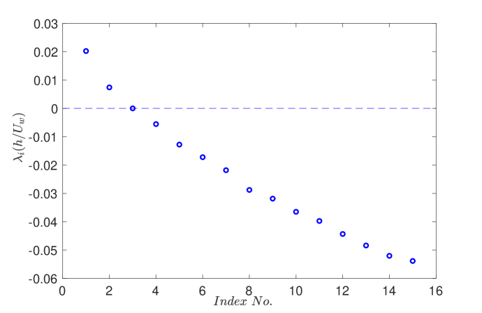
Figure 2: The first 15 Lyapunov exponents of the DNS mean flow for $n_{x}=1$.

The dynamical significance of $N_{4}$ in sustaining the turbulent state is revealed by comparing the perturbation energetics under the influence of the DNS mean flow $\mathbf{U}$ with and without the term $N_{4}$. This can be achieved by calculating the Lyapunov exponents $\lambda_{Lyap}$ of the $\mathbf{U}$ obtained from a DNS and the associated Lyapunov vectors together with the contributions of each of these Lyapunov vectors to the energy transfer rates $\dot{E}_{def,n_{x}}$, $\dot{E}_{dissip,n_{x}}$, $\dot{E}_{nonlin,n_{x}}$ and comparing these rates with and without the term $N_{4}$. Although the $N_{4}$ term is energetically neutral it may have a profound impact on the energetics by modifying the perturbations to extract more or less energy from the mean flow. Evidence that the term $N_{4}$ is not fundamental to sustaining the turbulence but instead the parametric mechanism of RNL is fundamentally responsible for maintaining DNS turbulence would be provided by the following four conditions: (i) the top Lyapunov exponent, $\lambda_{n_{x}}$, is associated with the same streamwise components $n_{x}$ of the turbulent field in RNL and DNS and is neutral after accounting for the transfer of energy to the other streamwise perturbation components, which would indicate that the turbulent state is regulated to neutralize the top Lyapunov vector growth rate (maximum Lyapunov exponent) coincident with the (necessary) neutralization of the state vector, ($\emph{i}i$) the transfer of energy from the mean flow by the top Lyapunov vector $\dot{E}_{def,n_{x}}$ should exceed that by the state vector indicating that $N_{4}$ has disrupted the Lyapunov vector making it less effective at transferring energy from the mean flow, ($\emph{i}ii$) the Lyapunov vectors span the energy and the energetics of the DNS perturbation field in a convincingly efficient manner, most tellingly if they span it in the order of their growth rate, and ($\emph{i}v$) in addition to supporting the perturbation energy and energetics the Lyapunov vectors support the roll circulation maintaining the coherent roll/streak structure.

Satisfying these conditions would strongly support the conclusion that the DNS turbulence is being maintained primarily through the parametric perturbation growth process associated with the temporal variation of $\mathbf{U}$ that supports turbulence in RNL, without substantial contribution from the $N_{4}$ nonlinearity. The alternative is that the $N_{4}$ term contributes at leading order to the energetics which would imply centrality in the dynamics of turbulence for the alternative role for $N_{4}$, which is to replenish the subset of perturbations lying in the directions of growth. This distinction in mechanism can be clarified by observing that, if instead of making the dynamically crucial choice of the streamwise average as the mean in constructing the RNL system and the mean flow were instead chosen to be the time-independent streamwise-spanwise-temporal mean, which in a boundary layer flow is the stable Reynolds-Tiederman profile Reynolds and Tiederman (1967), the $N_{4}$ nonlinearity must assume this role if turbulence is to be sustained. This follows because the alternative parametric mechanism would not be available. Turbulence could in principle be sustained by this mechanism if $N_{4}$ were sufficiently effective in scattering perturbations back into the directions of non-normal growth. However, the experiments of Jimenez & Pinelli Jiménez and Pinelli (1999) show that this is not the case. They demonstrate that removing the streak component in a DNS of a channel flow laminarizes the flow. Although the mean flow in their DNS remains highly non-normal the mechanism of nonlinear scattering back into the growing subspace of the non-normal operator can not maintain a turbulent state in the absence parametric mechanism made available by the specific structure of the fluctuating streak.

Figure 3: Contribution to the instantaneous energy growth rate of the $n_{x}=1$ perturbation component in DNS: extraction from the fluctuating $n_{x}=0$ mean component $\dot{E}_{lin,n_{x}}/(2E_{n_{x}})$ (blue, solid); loss to dissipation $\dot{E}_{dissip,n_{x}}/(2E_{n_{x}})$ (red, solid); transfer to the other $n_{x}>1$ streamwise components $\dot{E}_{nonlin,n_{x}}/(2E_{n_{x}})$ (green). The mean values of these rates are indicated with the dashed lines with the corresponding color. These average rates sum to $\lambda_{state}=0$. The corresponding rates for the first Lyapunov vector are shown in black and purple dash-dotted lines (there is no energy transfer to the other components as $N_{4}$ is absent in this calculation). These rates sum to the Lyapunov exponent $\lambda_{Lyap}=0.02U_{w}/h$, which is as expected positive and comparable to the transfer rate from the state vector, $\dot{E}_{nonlin,n_{x}}/(2E_{n_{x}})=0.04U_{w}/h$.

III The Lyapunov exponent of the mean flow in Couette turbulence at R=600

Table 1: The channel is periodic in the streamwise, $x$, and spanwise, $z$, direction and at the channel walls $y=\pm h$ the velocity is $\mathbf{u}=(\pm U_{w},0,0)$. The channel length is $L_{x}$ and $L_{z}$ in the streamwise and spanwise directions respectively. The number of streamwise and spanwise Fourier components is $N_{x}$ and $N_{z}$ after dealiasing in the streamwise and spanwise direction by the $2/3$ rule, and we use $N_{y}$ grid points in the wall-normal direction. $R=U_{w}h/\nu$ is the Reynolds number of the simulation, with $\nu$ the kinematic viscosity.

Parameter	$[L_{x},L_{z}]/h$	$N_{x}\times N_{z}\times N_{y}$	$R$
NS600	$[1.75\pi\;,\;1.2\pi]$	$17\times 17\times 35$	600

Consider a Couette turbulence simulation at $R=600$ in a periodic channel with parameters given in Table 1. This is a larger channel than the minimal Couette flow channel studied by Hamilton, Kim & Waleffe (Hamilton et al., 1995) at $R=400$. RNL turbulence with these parameters at $R=600$ was systematically examined recently (Farrell and Ioannou, 2017).

We first calculate the Lyapunov exponent $\lambda_{Lyap}$ of the DNS streamwise mean flow by estimating (8) from a long integration of (4) with the mean flow $\mathbf{U}$ obtained from a turbulent DNS. The initial state $\mathbf{u}^{\prime}$ is inconsequential because, with measure zero exception, any random initial condition converges in this system with exponential accuracy to the Lyapunov vector associated with the largest Lyapunov exponent. The full spectrum of Lyapunov exponents and vectors can be obtained by an orthogonalization procedure. For a discussion of the calculation and properties of Lyapunov exponents and the associated Lyapunov vectors refer to Refs. (Farrell and Ioannou, 1996, 1999, 2017; Wolfe and Samelson, 2007; Ding et al., 2016). Because of the streamwise independence of $\mathbf{U}$, the different streamwise Fourier components of $\mathbf{u}^{\prime}$ in this Lyapunov exponent calculation, in which the $N_{4}$ term is absent, evolve independently and the Lyapunov vector associated with a given Lyapunov exponent has streamwise structure confined to a single streamwise wavenumber $k_{x}=2\pi n_{x}h/L_{x}$, corresponding to the $n_{x}$ streamwise Fourier component.

The top Lyapunov exponent at each $n_{x}$ is shown in figure 1. This plot reveals that the time dependent streamwise mean flow $\mathbf{U}$ is asymptotically stable to all perturbations with $n_{x}>1$ with only the $n_{x}=1$ streamwise component supporting a positive Lyapunov exponent of $\lambda_{Lyap}\approx 0.02U_{w}/h$. Recall that in RNL the top Lyapunov exponent also has wavenumber $n_{x}=1$ and is exactly zero consistent with mean $\mathbf{U}$ being adjusted by feedback through the Reynolds stress term $N_{2}$ to exact neutrality. The top Lyapunov exponent obtained using the $\mathbf{U}$ of DNS is positive consistent with the requirement to account for the energy exported to other perturbations. Figure 2 shows that the DNS mean flow being without energy loss to scattering by the N4 term actually supports two positive Lyapunov exponents with $n_{x}=1$.

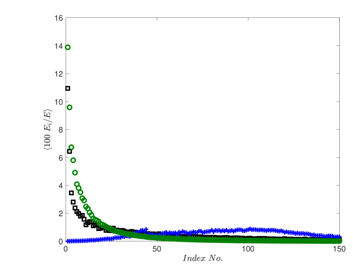
Figure 4: Average energy percentage of the $n_{x}=1$ flow accounted for by each Lyapunov vector (black squares). Average energy percentage of the $n_{x}=1$ flow accounted for by the eigenvectors of $A+A^{\dagger}$ ordered in descending order of their eigenvalue (blue crosses). $A$ is the operator in (4) governing the linear evolution of the perturbations about $\mathbf{U}$. The eigenvectors of $A+A^{\dagger}$ are the orthogonal directions of stationary instantaneous perturbation energy growth rate, with this growth rate given by the corresponding eigenvalue. The perturbation component of the turbulent flow is adjusted to have a small projection on the first eigenvectors of $A+A^{\dagger}$ associated with large instantaneous energy growth rates. Also shown is the energy percentage accounted for by the PODs of the $n_{x}=1$ component of the NL perturbation state (green circles).

Contributions to the Lyapunov exponent from mean flow energy transfer and from dissipation are plotted as a function of time in figure 3. The growth rate associated with energy transfer from the fluctuating streamwise mean is on average $0.11U_{w}/h$, while the dissipation rate is on average $0.09U_{w}/h$ resulting in the positive Lyapunov exponent $\lambda_{Lyap}=0.02U_{w}/h$. These transfers occur when perturbations evolve under the dynamics of the fluctuating streamwise mean flow $\mathbf{U}$ of the DNS but in the absence of two effects: (i) disturbance to the perturbation structure by the perturbation-perturbation nonlinearity $N_{4}$ and ($\emph{i}i$) transfer of energy to other perturbations by $N_{4}$. This result demonstrates that the parametric growth mechanism is able to maintain the perturbation turbulence component against dissipation with additional energy extraction to account for transfer to the other scales.

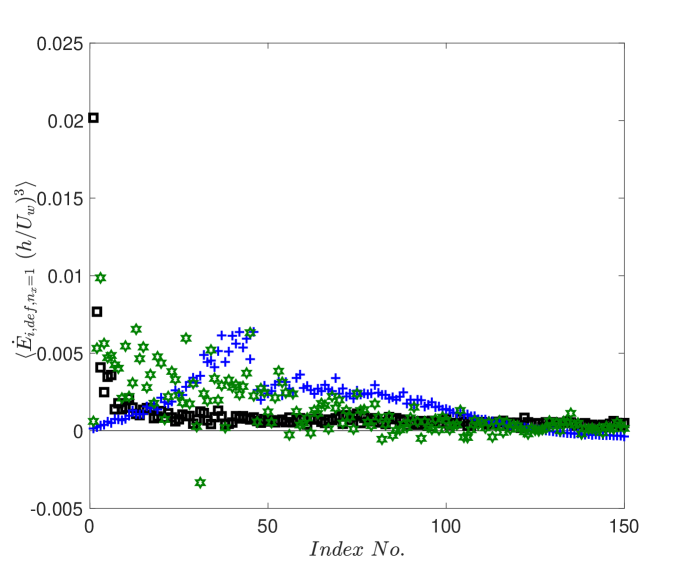
Figure 5: Contribution of the Lyapunov vectors (black squares), the PODs (green stars) and the eigenvectors of $A+A^{\dagger}$ (blue crosses) to the energy transfer rate, $\dot{E}_{lin}$, from the mean flow.

We now contrast the energetics of the Lyapunov vectors on the DNS mean flow just shown with the corresponding energetics of the $n_{x}=1$ Fourier component of the state vector obtained from the DNS itself in order to determine whether the $N_{4}$ term has the effect of influencing the perturbations to have a more or less favorable configuration for extracting energy from the mean flow. These results are also shown in figure 3 from which it can be seen that although the DNS turbulent state vector episodically exceeds its associated Lyapunov vector in rate of energy transfer from the mean flow this transfer rate with the influence of the $N_{4}$ term included is slightly less on average than that achieved by the first Lyapunov vector in the absence of the influence of $N_{4}$: energy transfer rate to the DNS state vector produces growth rate $0.099U_{w}/h$ compared to $0.107U_{w}/h$ for the Lyapunov vector on the DNS mean flow. This demonstrates that the nonlinear term $N_{4}$ does not configure the perturbations to transfer more energy from the highly non-normal streamwise mean flow $\mathbf{U}$ on average. However, despite the fact that the energy transferred from the streamwise mean flow by the DNS perturbation state and by the first Lyapunov vector are nearly equal when averaged over time, the correlation coefficient of the transfer rate time series, shown in figure 3, is low ($0.26$) suggesting that the $N_{4}$ term has disrupted the first Lyapunov vector and spread its energy to other Lyapunov vectors. The fact that this disruption does not substantially alter the time-mean energy transfer from the streamwise mean flow suggests that the time mean energetics resulting from projection on the Lyapunov vectors of $\mathbf{U}$ is not substantially altered by $N_{4}$ while the projection at an instant in time is. Note also that in the energetics of the $n_{x}=1$ perturbation component in DNS there is a term not present in the corresponding Lyapunov vector: the energy interchanged with the remaining $n_{x}\neq 0$ components, which is also shown in figure 3. The $n_{x}=1$ perturbation component of the DNS exports energy to the other streamwise components of the flow and this transfer contributes $0.04U_{w}/h$ at this wavenumber to the decay rate. This additional decay is just sufficient to reduce the mean growth rate of the DNS to the required value $\lambda_{state}=0$.

We conclude that the Lyapunov exponent of the fluctuating streamwise mean flow $\mathbf{U}$ in DNS turbulence has been adjusted to near neutrality and with energetics consistent with the parametric growth mechanism fully accounting for the maintenance of the perturbation component of the turbulent state. The perturbation-perturbation nonlinearity, $N_{4}$, does not configure the perturbations to extract more energy from the streamwise mean flow than in the absence of this term, implying that $N_{4}$ acts as a negative influence on the perturbation growth process. This is opposite to the mechanism in toy models of turbulence in which nonlinearity systematically configures perturbations to be more effective at exploiting the non-normality of the mean flow (cf. Trefethen et al. (1993)). The fact that the mean DNS flow has been adjusted to near neutrality of its first Lyapunov vector suggests this structure is controlling the parametric instability of the mean state and therefore that the first Lyapunov vector should be a dominant component of the perturbation state in the DNS. However, differences between the time series of the energy transfer rate by the DNS state vector and by the top Lyapunov vector of the associated mean state suggests that other (decaying) Lyapunov vectors have been excited by $N_{4}$. This will be examined in the next section.

IV Analysis of perturbation energetics by projection onto the Lyapunov vector basis

Despite the correspondence between the mean energetics of the DNS perturbation state and the mean energetics of the top Lyapunov vector calculated using the associated fluctuating streamwise mean flow it remains to explain why time series of perturbation growth rate for these shown in figure 3 reveal considerable differences. This suggests further analysis to clarify the relation between the perturbation state and the Lyapunov vectors. The orthogonality property imposed on the Lyapunov vectors makes them an attractive basis for analyzing the relation between perturbation structure and energetics. Expanding the $n_{x}=1$ DNS perturbation state $\hat{\mathbf{u}}^{\prime}$ in the basis of the orthonormal in energy $n_{x}=1$ Lyapunov vectors, $\mathbf{u}_{i}^{\prime}$:

$$\hat{\mathbf{u}}^{\prime}(t)=\sum_{i}a_{i}(t)\mathbf{u}_{i}^{\prime}(t),$$ (14)

with projection coefficient:

$$a_{i}(t)=\left\langle\mathbf{u}_{i}^{\prime}(t)\boldsymbol{\cdot}\hat{\mathbf{u}}^{\prime}(t)\right\rangle_{x,y,z},$$ (15)

we obtain that the contribution to the perturbation energy of Lyapunov vector $\mathbf{u}_{i}^{\prime}$ is $E_{i}=a^{2}_{i}(t)/2$. Projection of the energy of the $n_{x}=1$ component of the perturbation state on the first 150 Lyapunov vectors is shown in figure 4. The percentage of energy accounted for by projection on the most unstable Lyapunov vector is $11\%$, significantly larger than the energy in each of the remaining Lyapunov vectors. Adding the second unstable Lyapunov vector raises this value to $17.4\%$ and the first 100 $n_{x}=1$ Lyapunov vectors account for $82\%$ of the energy of the $n_{x}=1$ component of the perturbation state. In order to understand the significance of the Lyapunov vectors as a basis for representing the DNS perturbation state we have determined the orthonormal structures of the proper orthogonal decomposition (PODs) of the $n_{x}=1$ component of the DNS with the methods discussed in Ref. (Nikolaidis et al., 2016). Comparison of the perturbation energy projected on the Lyapunov and the canonical POD basis in Figure 4 demonstrates that the Lyapunov vectors provide a good representation of the DNS perturbation state. We note that the energy of the perturbation state is partitioned into the Lyapunov vectors in the order of their Lyapunov exponent, while the energy accounted for by the POD basis necessarily decrease monotonically with the order of the POD this is not required of the Lyapunov vectors and therefore this monotonic decrease provides evidence that the Lyapunov vectors are active agents in the perturbation energetics. On the other hand, note that the Lyapunov vectors are not constrained by optimality of the POD basis to be an inferior basis for spanning the energy, because the Lyapunov vectors are time dependent and could theoretically span all the perturbation energy, as indeed is the case in RNL for which the entire energy and energetics is accounted for by the first Lyapunov vector.

In figure 4 we also show the average projection of the DNS state on the eigenvectors of the operator $A+A^{\dagger}$ ordered in descending order of their eigenvalues. $A$ is the linear operator in (4) governing the evolution of the perturbations, $\mathbf{u}^{\prime}$, about $\mathbf{U}$. The eigenvectors of $A+A^{\dagger}$ form an orthonormal set of perturbation structures ordered decreasing in instantaneous energy growth rate in the flow, $\mathbf{U}$. Typically in turbulent flows both the Lyapunov vectors and the perturbation state have small projection on the first eigenvectors of $A+A^{\dagger}$, which are the structures producing greatest instantaneous energy growth rates. The turbulent mean flow $\mathbf{U}$ is such that perturbations that lead to large instantaneous growth rate have large wavenumber and are located in episodically occurring regions of high deformation. The top Lyapunov and state vectors are instead concentrated at larger scale with relatively small instantaneous growth rate. Small projection of the perturbation state on the directions of maximum instantaneous growth rate was previously seen in RNL simulations at $R=600$ (Farrell and Ioannou, 2017). What is remarkable and indicative of the fundamental role of the Lyapunov vectors in the dynamics of DNS is the ordering of the perturbation energy in the Lyapunov vectors. Despite the dynamic importance of the basis of the eigenvectors of $A+A^{\dagger}$ comparable ordering does not occur for this basis.

In RNL simulations at $R=600$ the perturbation turbulent state is entirely supported by the top Lyapunov vector and the energetics of the perturbation state consequently are the energetics of this single Lyapunov vector. The $N_{4}$ nonlinearity distributes the perturbation energy over a subspace spanned primarily by the leading Lyapunov vectors, as shown in figure 4. We can determine the distribution of the first $N$ Lyapunov vectors ordered in contribution to the perturbation state energy growth rate, $\dot{E}_{i,def}$ by calculating

$$\sum_{i=1}^{N}\dot{E}_{i,def}\stackrel{{\scriptstyle\mathrm{def}}}{{=}}\left\langle\mathbf{u}^{\prime}_{<}\boldsymbol{\cdot}\left(-\mathbf{U}\boldsymbol{\cdot}\boldsymbol{\nabla}\mathbf{u}^{\prime}_{<}-\mathbf{u}^{\prime}_{<}\boldsymbol{\cdot}\boldsymbol{\nabla}\mathbf{U}\right)\right\rangle_{x,y,z,t}~{},$$ (16)

where

$$\mathbf{u}^{\prime}_{<}(t)=Re\left(\sum_{\alpha=1}^{N}a_{\alpha}(t)\mathbf{u}^{\prime}_{\alpha}(t)e^{2\pi ix/L_{x}}\right),$$ (17)

is the projection of the $n_{x}=1$ perturbation state, given in (14), on the first $N$ Lyapunov vectors. From this calculation, we can obtain the incremental contribution to the perturbation energy growth, $\dot{E}_{i,def}$, of each Lyapunov vector. We can similarly determine the contribution of each of the eigenvectors of $A+A^{\dagger}$ and of the PODs to the energetics of the perturbation state. The results, shown in Fig. 5, reveal that the Lyapunov vectors provide the primary support for the perturbation energetics and their energetic contribution follows the Lyapunov vector growth rate ordering. If the $N_{4}$ term were dominant in determining the structures supporting the perturbation state the energetics of the turbulent state in the DNS would not be expected to so closely reflect the asymptotic structures of the Lyapunov vectors. Also note that the first 70 PODs, which contain $95\%$ of the perturbation energy, are responsible for most of the energetic transfers, but their contribution is not ordered as in the case of the Lyapunov vectors, actually it is almost white. Note also that the contribution of the first 45 eigenfunctions of $A+A^{\dagger}$ is in reverse order of their instantaneous growth rate.

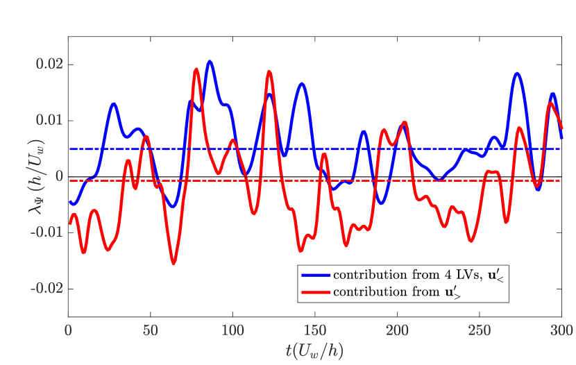
Figure 6: Time evolution of the contribution of the torques arising from the Reynolds stresses produced by $\mathbf{u}^{\prime}_{<}$ to maintenance of $\Psi^{2}$, which largely consists of the rolls (blue). The torques from $\mathbf{u}^{\prime}_{>}$ (red) make no net contribution to the rolls in this measure. The time mean contributions are indicated with dashed lines. This figure identifies the perturbation subspace responsible for maintaining the roll against dissipation to be the subspace spanned by the four least stable LVs.

V Analysis of the contribution of the Lyapunov vectors to the self -sustaining process

We have seen that the perturbation structure in a DNS has significant projection on the first LV ($11\%$ on average) and about $20\%$ on average on the subspace spanned by the four least stable LVs. These least stable Lyapunov vectors also dominate the others in the rate of energy extraction from the streamwise flow $\mathbf{U}(y,z,t)$. Remarkably, they also account fully for the forcing of the roll and therefore the SSP. In order to assess the contribution of the Lyapunov vectors to the roll forcing consider the equation for the streamwise component $\Omega_{x}=\Delta_{h}\Psi$ with $\Delta_{h}\stackrel{{\scriptstyle\mathrm{def}}}{{=}}\partial_{y}^{2}+\partial_{z}^{2}$, of the mean vorticity equation, which is obtained by taking the streamwise component of the curl of (2a):

$$\frac{D\Omega_{x}}{Dt}=\underbrace{-\left[(\partial^{2}_{y}-\partial^{2}_{z})\langle vw\rangle_{x}+\partial_{yz}\left(\langle w^{2}\rangle_{x}-\langle v^{2}\rangle_{x}\right)\right]}_{G_{\Omega_{x}}}+\nu\Delta_{h}\Omega_{x}~{},$$ (18)

where $D/Dt=\partial_{t}+\mathbf{U}\cdot\nabla$ is the substantial derivative on the streamwise mean flow. From (18) we see that if it were not for the streamwise mean torque from the perturbation Reynolds stresses, $G_{\Omega_{x}}$, the roll would decay. The contribution of perturbation Reynolds stresses to the rate of change of the normalized streamwise square vorticity can be measured by $\lambda_{\Omega_{x}}={\int_{V}{\Omega_{x}}G_{\Omega_{x}}dV}/({2\int_{V}\Omega_{x}^{2}dV})$, and similarly, if more emphasis is to be given to the large scales, we could use as a measure the contribution of the perturbation Reynolds stresses to the maintenance of the square of the streamfunction. This normalized measure of contribution to $\Psi^{2}$ is $\lambda_{\Psi}={\int_{V}{\Psi}G_{\Psi}dV}/({2\int_{V}\Psi^{2}dV})$, where $G_{\Psi}\stackrel{{\scriptstyle\mathrm{def}}}{{=}}\Delta_{h}^{-1}G_{\Omega_{x}}$ and $\Delta_{h}^{-1}$ is the inverse cross-stream/spanwise Laplacian. In order to analyze the contribution of the first few Lyapunov vectors to the maintenance of the roll component of the SSP we decompose the perturbation field $\mathbf{u}^{\prime}$ into its component, $\mathbf{u}_{<}^{\prime}$, projected on the subspace spanned by the 4 least damped energy orthonormal LVs, denoted $\mathbf{u}_{i}^{\prime}$, $i=1,2,3,4$ and the projection on the complement $\mathbf{u}_{>}^{\prime}$:

$$\mathbf{u}_{<}^{\prime}\stackrel{{\scriptstyle\mathrm{def}}}{{=}}\sum_{i=1}^{4}(\mathbf{u}^{\prime}\cdot\mathbf{u}_{i}^{\prime})\mathbf{u}_{i}^{\prime}~{},~{}~{}~{}\mathbf{u}_{>}^{\prime}\stackrel{{\scriptstyle\mathrm{def}}}{{=}}\mathbf{u}^{\prime}-\mathbf{u}_{<}^{\prime}~{},$$ (19)

and estimate $G_{\Psi}$ produced by $\mathbf{u}_{<}^{\prime}$ and $\mathbf{u}_{>}^{\prime}$. The contribution of these subspaces to $\lambda_{\Psi}$ is shown in Fig. 6. It can be seen that the first four least stable LVs contribute $100\%$ on average to the roll maintenance . This identification of a small subset of the least stable LVs as the perturbation structures that support the SSP anticipates laminarization of the turbulence in the DNS upon removal of this subspace (cf. Farrell et al. (2018)).

VI Conclusions

Analyses made using SSD systems closed at second order have demonstrated that a realistic self-sustained turbulent state is maintained by the parametric growth mechanism arising from interaction between the temporally and spanwise/cross-stream spatially varying streamwise-mean flow and the associated perturbation component Thomas et al. (2014, 2015); Farrell et al. (2016). In these second order SSD systems the streamwise-mean flow is necessarily adjusted exactly to neutral stability, with the understanding that the time dependent streamwise mean flow is considered neutral when the first Lyapunov exponent is zero. This result reinterprets the conjecture that the statistical state of inhomogeneous turbulence should have mean flow adjusted to neutral hydrodynamic stability.

In this work identification of the parametric mechanism supporting the perturbation component of turbulence obtained using SSD in the RNL system has been extended to DNS. While in the case of RNL support of the energy, energetics and the roll forcing is solely on the feedback neutralized first Lyapunov vector, in the case of DNS, energy, energetics and roll forcing are spread by nonlinearity over the Lyapunov vectors. Indicative that the Lyapunov vectors maintain their centrality in DNS dynamics is that support of the perturbation structure and energetics is ordered in the Lyapunov vectors descending in their associated exponents. The neutrality of the top Lyapunov vector in both RNL and DNS, when account is taken of the transfer of energy to other scales in the case of DNS, implies that the mean state neutrality conjecture for determining the statistical state is valid if neutrality of the mean state is reinterpreted as neutrality of the top Lyapunov vector(s). Consistent with the parametric mechanism sustaining the turbulence, the perturbation structure is concentrated on the top Lyapunov vectors of the time varying streamwise-mean flow and ordered in their Lyapunov exponents. Identification of the dynamical support of RNL and DNS turbulence to be the neutrally and stable Lyapunov vectors with associated parametric growth mechanism vindicates the conjecture that the mechanism that underlies turbulence in wall-bounded shear flow is parametric instability of the time and spanwise varying streamwise mean. Although essentially unstructured scattering by perturbation-perturbation nonlinearity constitutes a plausible mechanism by which the subspace of transiently growing perturbations is supported, we find the perturbation-perturbation nonlinearity does not configure the perturbations to extract more energy from the mean flow than they would in the absence of this term implying that the nonlinearity acts as a disruption to the parametric growth process supporting the perturbation field rather than augmenting the perturbation maintenance process. The perturbation-perturbation nonlinearity instead transfers energy to other Lyapunov vectors maintaining them as parametric energy extracting structures despite their negative exponents. These Lyapunov vectors that are being excited by scattering and maintained by extracting energy from the mean flow and are primarily responsible for the structure and maintenance of the perturbation field in contradistinction to the familiar implication of a perturbation cascade in this process.

We conclude that the mean flow in the DNS has been adjusted to Lyapunov neutrality and that the Lyapunov vectors support the energy, energetics and role in the SSP of the perturbation component of the turbulent state. These properties of the Lyapunov vectors verify that parametric growth on the fluctuating streamwise mean flow and its regulation by Reynolds stress feedback, which has been identified in RNL turbulence, is also the mechanism underlying the support of as well as the regulation to a statistical steady state of turbulence in the DNS.