Analysis of the $hp$-version of a first order system least squares method for the Helmholtz equation

Abstract

Extending the wavenumber-explicit analysis of chen-qiu17 , we analyze the $L^{2}$-convergence of a least squares method for the Helmholtz equation with wavenumber $k$. For domains with an analytic boundary, we obtain improved rates in the mesh size $h$ and the polynomial degree $p$ under the scale resolution condition that $hk/p$ is sufficiently small and $p/\log k$ is sufficiently large.

1 Introduction

We consider the following Helmholtz problem:

$$-\Delta u-k^{2}u =f\quad \text{in }\Omega,$$ (1)

$$\partial_{n}u-iku =g \text{on }\partial\Omega,$$

where $k\geq k_{0}>0$ is real. For large $k$, the numerical solution of (1) is challenging due to the requirement to resolve the oscillatory nature of the solution. A second challenge arises in classical, $H^{1}$-conforming discretizations of (1) from the fact that the Galerkin method is not an energy projection, and a meaningful approximation is only obtained under more stringent conditions on the mesh size $h$ and the polynomial degree $p$ than purely approximation theoretical considerations suggest. This shortcoming has been analyzed in the literature. In particular, as discussed in more detail in melenk-sauter11 ; esterhazy-melenk12 , the analyses ihlenburg98 ; ihlenburg-babuska95 ; ihlenburg-babuska97 ; ainsworth04 ; melenk-sauter10 ; melenk-sauter11 ; esterhazy-melenk12 show that high order methods are much better suited for the high-frequency case of large $k$ than low order methods. Alternatives to the classical Galerkin methods that are still based on high order methods include stabilized methods for Helmholtz feng-wu09 ; feng-wu11 ; feng-xing13 ; zhu-wu13 , hybridizable methods chen-lu-xu13 , least-squares type methods chen-qiu17 ; lee-manteuffel-mccormick-ruge00 and Discontinuous Petrov Galerkin methods, petrides-demkowicz17 ; demkowicz-gopalakrishnan-muga-zitelli12 . An attractive feature of least squares type methods is that the resulting linear system is always solvable and that they feature quasi-optimality, albeit in some nonstandard residual norms. In the present paper, we show for the least squares method (4) an a priori estimate in the more tractable $L^{2}(\Omega)$-norm under the scale resolution condition (35). For that, we closely follow chen-qiu17 . Our key refinement over chen-qiu17 is an improved regularity estimate for the solution of a suitable dual problem (cf. Lemma 1 vs. (chen-qiu17, , Lemma 5.1)) that allows us to establish the improved $p$-dependence in the $L^{2}(\Omega)$-error estimate (cf. Theorem 5.1 vs. (chen-qiu17, , Thm. 2.5)). As a tool, which is of independent interest, we develop approximation operators in Raviart-Thomas and Brezzi-Douglas-Marini spaces with optimal (in $h$ and $p$) approximation rates simultaneously in $L^{2}(\Omega)$ and $\boldsymbol{H}(\operatorname{div},\Omega)$.

Throughout this paper, if not otherwise stated, we assume the following:

Assumption 1.1

In spatial dimension $d=2,3$ the bounded Lipschitz domain $\Omega\subset\mathbb{R}^{d}$ has an analytic boundary. The wavenumber $k$ satisfies $k\geq k_{0}>0$. Furthermore $f\in L^{2}(\Omega)$ and $g\in L^{2}(\partial\Omega)$.

Remark 1

∎Under Assumption 1.1 we may apply (baskin-spence-wunsch16, , Thm. 1.8) to conclude that the solution $u\in H^{1}(\Omega)$ satisfies the a priori bound

$$\left\lVert u\right\rVert_{H^{1}(\Omega)}+k\left\lVert u\right\rVert_{L^{2}(\Omega)}\leq C(\left\lVert f\right\rVert_{L^{2}(\Omega)}+\left\lVert g\right\rVert_{L^{2}(\partial\Omega)}),$$ (2)

where $C>0$ is independent of $k$. ∎

Notation and preliminaries: Boldface letters like $\boldsymbol{V}$, $\boldsymbol{\varphi}$ and $\boldsymbol{\Pi}$ will be reserved for quantities having more than one spatial dimensions, while normal letters like $W$, $u$ and $\Pi$ will be used for quantities with one spatial dimension. The reference element will be denoted by $\widehat{K}$, whereas the physical one will just be denoted by $K$. In a similar way, we will distinguish between objects associated with the reference element and the physical one. A function defined on the reference element $\widehat{K}$ will therefore be denoted by $\hat{u}$, while a function defined on the physical element $K$ will be denoted by $u$. We will follow the same convention when it comes to operators acting on a function space. Therefore operators acting on functions defined on $\widehat{K}$ or $K$ will be denoted by $\widehat{\Pi}$ or $\Pi$ respectively. Generic constants will either be denoted by $C$ or hidden inside a $\lesssim$ and will be independent of the wavenumber $k$, the mesh size $h$ and the polynomial degree $p$, if not otherwise stated.

Outline: The outline of this paper is as follows. In Section 2 we introduce the first order system least squares (FOSLS) method itself, followed by Section 3, where we prove a refined duality argument (Lemma 1), which is later used to derive an a priori estimate (Theorem 5.1) of the method. Key ingredients are the results of melenk-parsania-sauter13 , where a frequency explicit splitting of the solution to (1) is performed when the data has higher order Sobolev regularity. Section 4 is concerned with the approximation properties of Raviart-Thomas and Brezzi-Douglas-Marini spaces. We therefore follow the methodology of melenk-sauter10 in order to construct approximation operators, which are not only $p$-optimal and approximate simultaneous in $L^{2}(\Omega)$ and $H^{1}(\Omega)$, but also admit an elementwise construction. Section 5 is then devoted to the a priori estimate. Concluding, we give numerical examples which compliment the theoretical findings and compare the method to the classical FEM in Section 6.

2 First order system least squares method and useful results

In the present Section we introduce the method of chen-qiu17 and list some useful results which are used later in the paper.

2.1 First order system least squares

We employ the complex Hilbert spaces

$$\boldsymbol{V}=\{\boldsymbol{\varphi}\in\boldsymbol{H}(\operatorname{div},\Omega)\colon\boldsymbol{\varphi}\cdot\boldsymbol{n}\in L^{2}(\partial\Omega)\}\quad\text{ and }\quad W=H^{1}(\Omega),$$

where $\boldsymbol{V}$ is endowed with the usual graph norm and $W$ with the classical $H^{1}(\Omega)$-norm. On $\boldsymbol{V}\times W$ we introduce the bilinear form $b$ and the linear functional $F$ by

$$b((\boldsymbol{\varphi},u),(\boldsymbol{\psi},v)) \coloneqq(ik\boldsymbol{\varphi}+\nabla u,ik\boldsymbol{\psi}+\nabla v)_{\Omega}+(iku+\nabla\cdot\boldsymbol{\varphi},ikv+\nabla\cdot\boldsymbol{\psi})_{\Omega}+$$

$$\phantom{\coloneqq}k(\boldsymbol{\varphi}\cdot\boldsymbol{n}+u,\boldsymbol{\psi}\cdot\boldsymbol{n}+v)_{\partial\Omega},$$

$$F((\boldsymbol{\psi},v)) \coloneqq(-ik^{-1}f,ikv+\nabla\cdot\boldsymbol{\psi})_{\Omega}+(ig,\boldsymbol{\psi}\cdot\boldsymbol{n}+v)_{\partial\Omega},$$

where $(u,v)_{\Omega}=\int_{\Omega}u\overline{v}\,\mathrm{d}x$. If $u\in H^{1}(\Omega)$ is the weak solution to (1) then the pair $(\boldsymbol{\varphi},u)$ with $\boldsymbol{\varphi}=ik^{-1}\nabla u$ is in fact in $\boldsymbol{V}\times W$ due to the assumed regularity of the data and the domain and therefore satisfies

$$b((\boldsymbol{\varphi},u),(\boldsymbol{\psi},v))=F((\boldsymbol{\psi},v))~{}~{}~{}\forall(\boldsymbol{\psi},v)\in\boldsymbol{V}\times W.$$ (3)

For a given regular mesh $\mathcal{T}_{h}$ we consider the finite element spaces $\boldsymbol{V}_{h}=\boldsymbol{\mathrm{RT}}_{p}(\mathcal{T}_{h})\subset\boldsymbol{V}$ or $\boldsymbol{V}_{h}=\boldsymbol{\mathrm{BDM}}_{p}(\mathcal{T}_{h})\subset\boldsymbol{V}$ and $W_{h}=S_{p}(\mathcal{T}_{h})\subset W$, where $\boldsymbol{\mathrm{RT}}_{p}(\mathcal{T}_{h})$ denotes the Raviart-Thomas space and $\boldsymbol{\mathrm{BDM}}_{p}(\mathcal{T}_{h})$ the Brezzi-Douglas-Marini space; see Section 4 for further detail and definitions. The FOSLS method is to find $(\boldsymbol{\varphi}_{h},u_{h})\in\boldsymbol{V}_{h}\times W_{h}$ such that

$$b((\boldsymbol{\varphi}_{h},u_{h}),(\boldsymbol{\psi}_{h},v_{h}))=F((\boldsymbol{\psi}_{h},v_{h}))~{}~{}~{}\forall(\boldsymbol{\psi}_{h},v_{h})\in\boldsymbol{V}_{h}\times W_{h}.$$ (4)

Remark 2

Based on the a priori estimate (2) reference (chen-qiu17, , Thm. 2.4) asserts the existence of $C>0$ independent of $k$ such that

$$\left\lVert\boldsymbol{\varphi}\right\rVert_{L^{2}(\Omega)}^{2}+\left\lVert u\right\rVert_{L^{2}(\Omega)}^{2}+k\left\lVert\boldsymbol{\varphi}\cdot\boldsymbol{n}+u\right\rVert_{L^{2}(\partial\Omega)}^{2}\leq Cb((\boldsymbol{\varphi},u),(\boldsymbol{\varphi},u)),\quad\forall(\boldsymbol{\varphi},u)\in\boldsymbol{V}\times W,$$

which immediately gives uniqueness. Together with the fact that the pair $(\boldsymbol{\varphi},u)$ with $\boldsymbol{\varphi}=ik^{-1}\nabla u$ is a solution, we have unique solvability of (3). ∎

2.2 Auxiliary results

We will need the following decomposition result for the refined duality argument in Lemma 1.

Proposition 1 ((melenk-parsania-sauter13, , Thm. 4.5) combined with (baskin-spence-wunsch16, , Thm. 1.8))

Let $\Omega\subset\mathbb{R}^{d},d\in\left\{2,3\right\}$, be a bounded Lipschitz domain with an analytic boundary. Fix $s\in\mathbb{N}_{0}$. Then there exist constants $C,\gamma>0$ independent of $k$ such that for every $f\in H^{s}(\Omega)$ and $g\in H^{s+1/2}(\partial\Omega)$ the solution $u=S_{k}(f,g)$ of (1) can be written as $u=u_{A}+u_{H^{s+2}}$, where, for all $n\in\mathbb{N}_{0}$, there holds

$$\left\lVert u_{A}\right\rVert_{H^{1}(\Omega)}+k\left\lVert u_{A}\right\rVert_{L^{2}(\Omega)}\leq C (\left\lVert f\right\rVert_{L^{2}(\Omega)}+\left\lVert g\right\rVert_{H^{1/2}(\partial\Omega)}),$$ (5)

$$\left\lVert\nabla^{n+2}u_{A}\right\rVert_{L^{2}(\Omega)}\leq C\gamma^{n}k^{-1}\max\left\{n,k\right\}^{n+2} (\left\lVert f\right\rVert_{L^{2}(\Omega)}+\left\lVert g\right\rVert_{H^{1/2}(\partial\Omega)}),$$ (6)

$$\left\lVert u_{H^{s+2}}\right\rVert_{H^{s+2}(\Omega)}+k^{s+2}\left\lVert u_{H^{s+2}}\right\rVert_{L^{2}(\Omega)}\leq C (\left\lVert f\right\rVert_{H^{s}(\Omega)}+\left\lVert g\right\rVert_{H^{s+1/2}(\partial\Omega)}).$$ (7)

Remark 3

∎Interpolation between $L^{2}(\Omega)$ and $H^{s+2}(\Omega)$ in Proposition 1 gives estimates for lower order Sobolev norms: Since we have for any $v\in H^{m}(\Omega)$

$$\left\lVert v\right\rVert_{H^{j}(\Omega)}\leq C\left\lVert v\right\rVert_{H^{m}(\Omega)}^{\frac{j}{m}}\left\lVert v\right\rVert_{L^{2}(\Omega)}^{\frac{m-j}{m}},\qquad j\in\{0,\dots,m\},$$

Proposition 1 implies for $j\in\{0,\dots,s+2\}$

$$k^{s+2-j}\left\lVert u_{H^{s+2}}\right\rVert_{H^{j}(\Omega)}\leq C(\left\lVert f\right\rVert_{H^{s}(\Omega)}+\left\lVert g\right\rVert_{H^{s+1/2}(\partial\Omega)}).$$

∎

Furthermore we often use the multiplicative trace inequality. We remind the reader of the general form, even though we only need it in the special case $s=1$.

Proposition 2 ((melenk05, , Thm. A.2))

Let $\Omega\subset\mathbb{R}^{d}$ be a Lipschitz domain and $s\in(1/2,1]$. Then there exists a constant $C>0$ such that for all $u\in H^{s}(\Omega)$ there holds

$$\left\lVert u\right\rVert_{L^{2}(\partial\Omega)}\leq C\left\lVert u\right\rVert_{L^{2}(\Omega)}^{1-1/(2s)}\left\lVert u\right\rVert_{H^{s}(\Omega)}^{1/(2s)},$$

where the left-hand side is understood in the trace sense.

3 Duality Argument

We extend the results of (chen-qiu17, , Lemma 5.1) by showing that the function $\boldsymbol{\psi}_{H^{2}}\in\boldsymbol{H}^{1}(\operatorname{div},\Omega)$, constructed therein, can actually be modified to satisfy $\boldsymbol{\psi}_{H^{2}}\in\boldsymbol{H}^{2}(\Omega)$ and still allow for wavenumber-explicit higher order Sobolev norm estimates.

Lemma 1

For any $(\boldsymbol{\varphi},w)\in\boldsymbol{V}\times W$ there exists $(\boldsymbol{\psi},v)\in\boldsymbol{V}\times W$ such that $\left\lVert w\right\rVert_{L^{2}(\Omega)}^{2}=b((\boldsymbol{\varphi},w),(\boldsymbol{\psi},v))$. The pair $(\boldsymbol{\psi},v)$ admits a decomposition $\boldsymbol{\psi}=\boldsymbol{\psi}_{A}+\boldsymbol{\psi}_{H^{2}}$, $v=v_{A}+v_{H^{2}}$, where $\boldsymbol{\psi}_{A}$ and $v_{A}$ are analytic in $\Omega$, $\boldsymbol{\psi}_{H^{2}}\in\boldsymbol{H}^{2}(\Omega)$, and $v_{H^{2}}\in H^{2}(\Omega)$. Furthermore there exist constants $C,\gamma>0$ independent of $k$ such that for all $n\in\mathbb{N}_{0}$

$$\left\lVert\boldsymbol{\psi}_{A}\right\rVert_{H^{1}(\Omega)}+k\left\lVert\boldsymbol{\psi}_{A}\right\rVert_{L^{2}(\Omega)} \leq Ck\left\lVert w\right\rVert_{L^{2}(\Omega)},$$ (8)

$$\left\lVert v_{A}\right\rVert_{H^{1}(\Omega)}+k\left\lVert v_{A}\right\rVert_{L^{2}(\Omega)} \leq Ck\left\lVert w\right\rVert_{L^{2}(\Omega)},$$ (9)

$$\left\lVert\nabla^{n+2}\boldsymbol{\psi}_{A}\right\rVert_{L^{2}(\Omega)}+\left\lVert\nabla^{n+2}v_{A}\right\rVert_{L^{2}(\Omega)} \leq C\gamma^{n}\max\left\{n,k\right\}^{n+2}\left\lVert w\right\rVert_{L^{2}(\Omega)},$$ (10)

$$\!\!\!\!\!\!\left\lVert\boldsymbol{\psi}_{H^{2}}\right\rVert_{H^{2}(\Omega)}+k\left\lVert\boldsymbol{\psi}_{H^{2}}\right\rVert_{H^{1}(\Omega)}+k^{2}\left\lVert\boldsymbol{\psi}_{H^{2}}\right\rVert_{L^{2}(\Omega)} \leq C\left\lVert w\right\rVert_{L^{2}(\Omega)},$$ (11)

$$\left\lVert v_{H^{2}}\right\rVert_{H^{2}(\Omega)}+k\left\lVert v_{H^{2}}\right\rVert_{H^{1}(\Omega)}+k^{2}\left\lVert v_{H^{2}}\right\rVert_{L^{2}(\Omega)} \leq C\left\lVert w\right\rVert_{L^{2}(\Omega)}.$$ (12)

Proof

∎The proof follows the ideas of (chen-qiu17, , Lemma 5.1); for the readers’ convenience we recapitulate the important steps of the proof. The novelty over chen-qiu17 is the ability to choose $\boldsymbol{\psi}_{H^{2}}\in\boldsymbol{H}^{2}(\Omega)$ together with $\left\lVert\boldsymbol{\psi}_{H^{2}}\right\rVert_{H^{2}(\Omega)}\leq C\left\lVert w\right\rVert_{L^{2}(\Omega)}$.

Consider the problem

$$-\Delta z-k^{2}z =w\qquad \text{in }\Omega,$$

$$\partial_{n}z+ikz =0 \text{on }\partial\Omega.$$

For any $\boldsymbol{\varphi}\in\boldsymbol{V}$ we have, using the weak formulation and integrating by parts,

$$\left\lVert w\right\rVert_{L^{2}(\Omega)}^{2} =(\nabla w,\nabla z)_{\Omega}-k^{2}(w,z)_{\Omega}-ik(w,z)_{\partial\Omega}$$

$$=(ik\boldsymbol{\varphi}+\nabla w,\nabla z)_{\Omega}-(ik\boldsymbol{\varphi},\nabla z)_{\Omega}-k^{2}(w,z)_{\Omega}-ik(w,z)_{\partial\Omega}$$

$$=(ik\boldsymbol{\varphi}+\nabla w,\nabla z)_{\Omega}+(\nabla\cdot\boldsymbol{\varphi}+ikw,-ikz)_{\Omega}+(\boldsymbol{\varphi}\cdot\boldsymbol{n}+w,ikz)_{\partial\Omega}.$$

Applying Proposition 1 together with Remark 3 we decompose $z$ into $z=z_{A}+z_{H^{2}}$ with $z_{A}$ analytic and $z_{H^{2}}\in H^{2}(\Omega)$. Furthermore we have, for all $n\in{\mathbb{N}}_{0}$,

$$\left\lVert z_{A}\right\rVert_{H^{1}(\Omega)}+k\left\lVert z_{A}\right\rVert_{L^{2}(\Omega)}\leq C \left\lVert w\right\rVert_{L^{2}(\Omega)},$$ (13)

$$\left\lVert\nabla^{n+2}z_{A}\right\rVert_{L^{2}(\Omega)}\leq C\gamma^{n}k^{-1}\max\left\{n,k\right\}^{n+2} \left\lVert w\right\rVert_{L^{2}(\Omega)},$$ (14)

$$\left\lVert z_{H^{2}}\right\rVert_{H^{2}(\Omega)}+k\left\lVert z_{H^{2}}\right\rVert_{H^{1}(\Omega)}+k^{2}\left\lVert z_{H^{2}}\right\rVert_{L^{2}(\Omega)}\leq C \left\lVert w\right\rVert_{L^{2}(\Omega)}.$$ (15)

Let $(\boldsymbol{\psi},v)\in\boldsymbol{V}\times W$ solve

$$ik\boldsymbol{\psi}+\nabla v =\nabla z\qquad \text{in }\Omega,$$

$$ikv+\nabla\cdot\boldsymbol{\psi} =-ikz\qquad \text{in }\Omega,$$

$$k^{1/2}(\boldsymbol{\psi}\cdot\boldsymbol{n}+v) =ik^{1/2}z\qquad \text{on }\partial\Omega.$$

Indeed, this system is uniquely solvable by Remark 2. This gives the desired representation such that $\left\lVert w\right\rVert_{L^{2}(\Omega)}^{2}=b((\boldsymbol{\varphi},w),(\boldsymbol{\psi},v))$. Using the decomposition $z=z_{A}+z_{H^{2}}$ we obtain $(\boldsymbol{\psi},v)=(\tilde{\boldsymbol{\psi}}_{A},\tilde{v}_{A})+(\tilde{\boldsymbol{\psi}}_{H^{2}},\tilde{v}_{H^{2}})$, where

$\displaystyle ik\tilde{\boldsymbol{\psi}}_{A}+\nabla\tilde{v}_{A}$ $\displaystyle=\nabla z_{A}\qquad$ $\displaystyle\text{in }\Omega,$ $\displaystyle ik\tilde{v}_{A}+\nabla\cdot\tilde{\boldsymbol{\psi}}_{A}$ $\displaystyle=-ikz_{A}\qquad$ $\displaystyle\text{in }\Omega,$ $\displaystyle k^{1/2}(\tilde{\boldsymbol{\psi}}_{A}\cdot\boldsymbol{n}+\tilde{v}_{A})$ $\displaystyle=ik^{1/2}z_{A}\qquad$ $\displaystyle\text{on }\partial\Omega,$ $\displaystyle ik\tilde{\boldsymbol{\psi}}_{H^{2}}+\nabla\tilde{v}_{H^{2}}$ $\displaystyle=\nabla z_{H^{2}}\qquad$ $\displaystyle\text{in }\Omega,$ $\displaystyle ik\tilde{v}_{H^{2}}+\nabla\cdot\tilde{\boldsymbol{\psi}}_{H^{2}}$ $\displaystyle=-ikz_{H^{2}}\qquad$ $\displaystyle\text{in }\Omega,$ $\displaystyle k^{1/2}(\tilde{\boldsymbol{\psi}}_{H^{2}}\cdot\boldsymbol{n}+\tilde{v}_{H^{2}})$ $\displaystyle=ik^{1/2}z_{H^{2}}\qquad$ $\displaystyle\text{on }\partial\Omega.$

One can immediately verify that

$$-\Delta(\tilde{v}_{A}-z_{A})-k^{2}(\tilde{v}_{A}-z_{A}) =2k^{2}z_{A}\qquad\qquad \text{in }\Omega,$$ (16)

$$\partial_{n}(\tilde{v}_{A}-z_{A})-ik(\tilde{v}_{A}-z_{A}) =(1+i)kz_{A}\qquad \text{on }\partial\Omega,$$

as well as

$$-\Delta(\tilde{v}_{H^{2}}-z_{H^{2}})-k^{2}(\tilde{v}_{H^{2}}-z_{H^{2}}) =2k^{2}z_{H^{2}}\qquad\qquad \text{in }\Omega,$$ (17)

$$\partial_{n}(\tilde{v}_{H^{2}}-z_{H^{2}})-ik(\tilde{v}_{H^{2}}-z_{H^{2}}) =(1+i)kz_{H^{2}}\qquad \text{on }\partial\Omega.$$

Note that the right-hand sides in equation (16) are analytic. This fact is used in (chen-qiu17, , Lemma 5.1, Lemma 4.4) to prove the following bounds for all $n\in{\mathbb{N}}_{0}$:

$$\left\lVert\nabla^{n+2}\tilde{v}_{A}\right\rVert_{L^{2}(\Omega)} \leq C\gamma^{n}\max\left\{n,k\right\}^{n+2}\left\lVert w\right\rVert_{L^{2}(\Omega)},$$ (18)

$$\left\lVert\tilde{v}_{A}\right\rVert_{H^{1}(\Omega)}+k\left\lVert\tilde{v}_{A}\right\rVert_{L^{2}(\Omega)} \leq Ck\left\lVert w\right\rVert_{L^{2}(\Omega)},$$ (19)

$$\left\lVert\nabla^{n+2}\tilde{\boldsymbol{\psi}}_{A}\right\rVert_{L^{2}(\Omega)} \leq C\gamma^{n}\max\left\{n,k\right\}^{n+2}\left\lVert w\right\rVert_{L^{2}(\Omega)},$$ (20)

$$\left\lVert\tilde{\boldsymbol{\psi}}_{A}\right\rVert_{H^{1}(\Omega)}+k\left\lVert\tilde{\boldsymbol{\psi}}_{A}\right\rVert_{L^{2}(\Omega)} \leq Ck\left\lVert w\right\rVert_{L^{2}(\Omega)}.$$ (21)

Since $\tilde{v}_{H^{2}}-z_{H^{2}}=S_{k}(2k^{2}z_{H^{2}},(1+i)kz_{H^{2}})$, where $S_{k}$ denotes the solution operator for (1), we can exploit the regularity of the right-hand sides in equation (17). Applying Proposition 1 with $s=1$ as well as Remark 3 we decompose $\tilde{v}_{H^{2}}-z_{H^{2}}=\hat{v}_{A}+\hat{v}_{H^{3}}$, where $\hat{v}_{A}$ is analytic and $\hat{v}_{H^{3}}\in H^{3}(\Omega)$. For every $j\in\left\{0,1,2,3\right\}$ we have

$$k^{3-j}\left\lVert\hat{v}_{H^{3}}\right\rVert_{H^{j}(\Omega)} \lesssim\left\lVert 2k^{2}z_{H^{2}}\right\rVert_{H^{1}(\Omega)}+\left\lVert(1+i)kz_{H^{2}}\right\rVert_{H^{3/2}(\partial\Omega)}$$

$$\lesssim\underbrace{k^{2}\left\lVert z_{H^{2}}\right\rVert_{H^{1}(\Omega)}}_{\stackrel{{\scriptstyle\eqref{bernkopf_melenk_eq:z_h_2_part}}}{{\lesssim}}k\left\lVert w\right\rVert_{L^{2}(\Omega)}}+\underbrace{k\left\lVert z_{H^{2}}\right\rVert_{H^{3/2}(\partial\Omega)}}_{\lesssim k\left\lVert z_{H^{2}}\right\rVert_{H^{2}(\Omega)}\stackrel{{\scriptstyle\eqref{bernkopf_melenk_eq:z_h_2_part}}}{{\lesssim}}k\left\lVert w\right\rVert_{L^{2}(\Omega)}}$$

$$\lesssim k\left\lVert w\right\rVert_{L^{2}(\Omega)}.$$

Summarizing the above we have

$$k^{-1}\left\lVert\hat{v}_{H^{3}}\right\rVert_{H^{3}(\Omega)}+\left\lVert\hat{v}_{H^{3}}\right\rVert_{H^{2}(\Omega)}+k\left\lVert\hat{v}_{H^{3}}\right\rVert_{H^{1}(\Omega)}+k^{2}\left\lVert\hat{v}_{H^{3}}\right\rVert_{L^{2}(\Omega)}\leq C\left\lVert w\right\rVert_{L^{2}(\Omega)}.$$ (22)

In order to analyze the behavior of $\hat{v}_{A}$ we first estimate

$$\left\lVert 2k^{2}z_{H^{2}}\right\rVert_{L^{2}(\Omega)}+\left\lVert(1+i)kz_{H^{2}}\right\rVert_{H^{1/2}(\partial\Omega)}\stackrel{{\scriptstyle\eqref{bernkopf_melenk_eq:z_h_2_part}}}{{\lesssim}}\left\lVert w\right\rVert_{L^{2}(\Omega)}.$$

We therefore conclude, again with Proposition 1, that

$$\left\lVert\hat{v}_{A}\right\rVert_{H^{1}(\Omega)}+k\left\lVert\hat{v}_{A}\right\rVert_{L^{2}(\Omega)} \leq C\left\lVert w\right\rVert_{L^{2}(\Omega)},$$ (23)

$$\left\lVert\nabla^{n+2}\hat{v}_{A}\right\rVert_{L^{2}(\Omega)} \leq C\gamma^{n}k^{-1}\max\left\{n,k\right\}^{n+2}\left\lVert w\right\rVert_{L^{2}(\Omega)}.$$ (24)

We turn to the final decompositions with associated norm bounds.

Final decomposition of $v$:

$$v=\tilde{v}_{A}+\tilde{v}_{H^{2}}=\tilde{v}_{A}+\underbrace{\tilde{v}_{H^{2}}-z_{H^{2}}}_{=\hat{v}_{A}+\hat{v}_{H^{3}}}+z_{H^{2}}=\underbrace{\tilde{v}_{A}+\hat{v}_{A}}_{\eqqcolon v_{A}}+\underbrace{\hat{v}_{H^{3}}+z_{H^{2}}}_{\eqqcolon v_{H^{2}}}.$$

Verification of (9):

$$\left\lVert v_{A}\right\rVert_{H^{1}(\Omega)}+k\left\lVert v_{A}\right\rVert_{L^{2}(\Omega)} \leq\underbrace{\left\lVert\tilde{v}_{A}\right\rVert_{H^{1}(\Omega)}+k\left\lVert\tilde{v}_{A}\right\rVert_{L^{2}(\Omega)}}_{\stackrel{{\scriptstyle\eqref{bernkopf_melenk_eq:v_A_tilde_low_derivatives}}}{{\leq}}Ck\left\lVert w\right\rVert_{L^{2}(\Omega)}}+\underbrace{\left\lVert\hat{v}_{A}\right\rVert_{H^{1}(\Omega)}+k\left\lVert\hat{v}_{A}\right\rVert_{L^{2}(\Omega)}}_{\stackrel{{\scriptstyle\eqref{bernkopf_melenk_eq:v_A_hat_low_derivatives}}}{{\leq}}C\left\lVert w\right\rVert_{L^{2}(\Omega)}}$$

$$\leq Ck\left\lVert w\right\rVert_{L^{2}(\Omega)}.$$

Verification of (12):

$$\left\lVert v_{H^{2}}\right\rVert_{H^{2}(\Omega)} +k\left\lVert v_{H^{2}}\right\rVert_{H^{1}(\Omega)}+k^{2}\left\lVert v_{H^{2}}\right\rVert_{L^{2}(\Omega)}$$

$$\leq\underbrace{\left\lVert\hat{v}_{H^{3}}\right\rVert_{H^{2}(\Omega)}+k\left\lVert\hat{v}_{H^{3}}\right\rVert_{H^{1}(\Omega)}+k^{2}\left\lVert\hat{v}_{H^{3}}\right\rVert_{L^{2}(\Omega)}}_{\stackrel{{\scriptstyle\eqref{bernkopf_melenk_eq:v_h_3_hat_low_derivatives}}}{{\leq}}C\left\lVert w\right\rVert_{L^{2}(\Omega)}}$$

$$\phantom{\leq}+\underbrace{\left\lVert z_{H^{2}}\right\rVert_{H^{2}(\Omega)}+k\left\lVert z_{H^{2}}\right\rVert_{H^{1}(\Omega)}+k^{2}\left\lVert z_{H^{2}}\right\rVert_{L^{2}(\Omega)}}_{\stackrel{{\scriptstyle\eqref{bernkopf_melenk_eq:z_h_2_part}}}{{\leq}}C\left\lVert w\right\rVert_{L^{2}(\Omega)}}$$

$$\leq C\left\lVert w\right\rVert_{L^{2}(\Omega)}.$$

Final decomposition of $\boldsymbol{\psi}$: Since $-ik\tilde{\boldsymbol{\psi}}_{H^{2}}=\nabla(\tilde{v}_{H^{2}}-z_{H^{2}})=\nabla\hat{v}_{A}+\nabla\hat{v}_{H^{3}}$, we decompose $\tilde{\boldsymbol{\psi}}_{H^{2}}=\hat{\boldsymbol{\psi}}_{A}+\hat{\boldsymbol{\psi}}_{H^{2}}$ accordingly such that $-ik\hat{\boldsymbol{\psi}}_{A}=\nabla\hat{v}_{A}$ and consequently $-ik\hat{\boldsymbol{\psi}}_{H^{2}}=\nabla\hat{v}_{H^{3}}$. The final decomposition takes the form

$$\boldsymbol{\psi}=\tilde{\boldsymbol{\psi}}_{A}+\tilde{\boldsymbol{\psi}}_{H^{2}}=\underbrace{\tilde{\boldsymbol{\psi}}_{A}+\hat{\boldsymbol{\psi}}_{A}}_{\eqqcolon\boldsymbol{\psi}_{A}}+\underbrace{\hat{\boldsymbol{\psi}}_{H^{2}}}_{\eqqcolon\boldsymbol{\psi}_{H^{2}}}.$$

Verification of (8):

$$\left\lVert\boldsymbol{\psi}_{A}\right\rVert_{H^{1}(\Omega)} +k\left\lVert\boldsymbol{\psi}_{A}\right\rVert_{L^{2}(\Omega)}$$

$$\leq\underbrace{\left\lVert\tilde{\boldsymbol{\psi}}_{A}\right\rVert_{H^{1}(\Omega)}+k\left\lVert\tilde{\boldsymbol{\psi}}_{A}\right\rVert_{L^{2}(\Omega)}}_{\stackrel{{\scriptstyle\eqref{bernkopf_melenk_eq:psi_A_tilde_low_derivatives}}}{{\leq}}Ck\left\lVert w\right\rVert_{L^{2}(\Omega)}}+\left\lVert\hat{\boldsymbol{\psi}}_{A}\right\rVert_{H^{1}(\Omega)}+k\left\lVert\hat{\boldsymbol{\psi}}_{A}\right\rVert_{L^{2}(\Omega)}$$

$$\leq Ck\left\lVert w\right\rVert_{L^{2}(\Omega)}+k^{-1}\left\lVert\nabla\hat{v}_{A}\right\rVert_{H^{1}(\Omega)}+\left\lVert\nabla\hat{v}_{A}\right\rVert_{L^{2}(\Omega)}$$

$$\leq Ck\left\lVert w\right\rVert_{L^{2}(\Omega)}+k^{-1}\underbrace{\left\lVert\hat{v}_{A}\right\rVert_{H^{1}(\Omega)}}_{\stackrel{{\scriptstyle\eqref{bernkopf_melenk_eq:v_A_hat_low_derivatives}}}{{\leq}}C\left\lVert w\right\rVert_{L^{2}(\Omega)}}+k^{-1}\underbrace{\left\lVert\nabla^{2}\hat{v}_{A}\right\rVert_{L^{2}(\Omega)}}_{\stackrel{{\scriptstyle\eqref{bernkopf_melenk_eq:v_A_hat_high_derivatives}}}{{\leq}}Ck\left\lVert w\right\rVert_{L^{2}(\Omega)}}+\underbrace{\left\lVert\hat{v}_{A}\right\rVert_{H^{1}(\Omega)}}_{\stackrel{{\scriptstyle\eqref{bernkopf_melenk_eq:v_A_hat_low_derivatives}}}{{\leq}}C\left\lVert w\right\rVert_{L^{2}(\Omega)}}$$

$$\leq Ck\left\lVert w\right\rVert_{L^{2}(\Omega)}.$$

Verification of (10): This is an immediate consequence of (18), (20), (24), and the fact that $-ik\hat{\boldsymbol{\psi}}_{A}=\nabla\hat{v}_{A}$.

Verification of (11): Since $-ik\hat{\boldsymbol{\psi}}_{H^{2}}=\nabla\hat{v}_{H^{3}}$ we estimate

$$\left\lVert\boldsymbol{\psi}_{H^{2}}\right\rVert_{H^{2}(\Omega)} +k\left\lVert\boldsymbol{\psi}_{H^{2}}\right\rVert_{H^{1}(\Omega)}+k^{2}\left\lVert\boldsymbol{\psi}_{H^{2}}\right\rVert_{L^{2}(\Omega)}$$

$$=k^{-1}\left\lVert\nabla\hat{v}_{H^{3}}\right\rVert_{H^{2}(\Omega)}+\left\lVert\nabla\hat{v}_{H^{3}}\right\rVert_{H^{1}(\Omega)}+k\left\lVert\nabla\hat{v}_{H^{3}}\right\rVert_{L^{2}(\Omega)}$$

$$\leq\underbrace{k^{-1}\left\lVert\hat{v}_{H^{3}}\right\rVert_{H^{3}(\Omega)}+\left\lVert\hat{v}_{H^{3}}\right\rVert_{H^{2}(\Omega)}+k\left\lVert\hat{v}_{H^{3}}\right\rVert_{H^{1}(\Omega)}}_{\stackrel{{\scriptstyle\eqref{bernkopf_melenk_eq:v_h_3_hat_low_derivatives}}}{{\leq}}C\left\lVert w\right\rVert_{L^{2}(\Omega)}}$$

$$\leq C\left\lVert w\right\rVert_{L^{2}(\Omega)},$$

which concludes the proof. ∎

4 Approximation properties of Raviart-Thomas and Brezzi-Douglas-Marini spaces

In the present Section we analyze the approximation properties of Raviart-Thomas and Brezzi-Douglas-Marini spaces. To that end, we first state some standard assumptions on the mesh and recall the relevant function spaces. Next, we will prove the existence of a polynomial approximation operator acting on functions defined on the reference element having certain desirable properties, as outlined below. This operator will then be used to construct a global polynomial approximation operator by means of the Piola transformation.

4.1 Preliminaries

We start with assumptions on the triangulation.

Assumption 4.1 (quasi-uniform regular meshes)

Let $\widehat{K}$ be the reference simplex. Each element map $F_{K}\colon\widehat{K}\to K$ can be written as $F_{K}=R_{K}\circ A_{K}$, where $A_{K}$ is an affine map and the maps $R_{K}$ and $A_{K}$ satisfy, for constants $C_{\mathrm{affine}},C_{\mathrm{metric}},\gamma>0$ independent of $K$:

$$\left\lVert A^{\prime}_{K}\right\rVert_{L^{\infty}(\widehat{K})}\leq C_{\mathrm{affine}}h_{K},\qquad \left\lVert(A^{\prime}_{K})^{-1}\right\rVert_{L^{\infty}(\widehat{K})}\leq C_{\mathrm{affine}}h^{-1}_{K},$$

$$\left\lVert(R^{\prime}_{K})^{-1}\right\rVert_{L^{\infty}(\tilde{K})}\leq C_{\mathrm{metric}},\qquad \left\lVert\nabla^{n}R_{K}\right\rVert_{L^{\infty}(\tilde{K})}\leq C_{\mathrm{metric}}\gamma^{n}n!\qquad\forall n\in\mathbb{N}_{0}.$$

Here, $\tilde{K}=A_{K}(\widehat{K})$ and $h_{K}>0$ denotes the element diameter.

We recall the definition of the Sobolev space $H_{00}^{1/2}(\omega)$. If $\omega$ is an edge of a triangle or face of a tetrahedron, then the norm $\left\lVert\cdot\right\rVert_{H_{00}^{1/2}(\omega)}$ is given by

$$\left\lVert u\right\rVert_{H_{00}^{1/2}(\omega)}^{2}\coloneqq\left\lVert u\right\rVert_{H^{1/2}(\omega)}^{2}+\left\lVert\frac{u}{\sqrt{\mathrm{dist}(\cdot,\partial\omega)}}\right\rVert_{L^{2}(\omega)}^{2},$$

and the space $H_{00}^{1/2}(\omega)$ is the completion of $C_{0}^{\infty}(\omega)$ under this norm. Since this norm is induced by a scalar product the space $H_{00}^{1/2}(\omega)$ is a Hilbert space.

On the reference element $\widehat{K}$ we introduce the Raviart-Thomas and Brezzi-Douglas-Marini elements of degree $p\geq 0$ in dimension $d$:

$$\mathcal{P}_{p}(\widehat{K}) \coloneqq\mathrm{span}\left\{\boldsymbol{x}^{\boldsymbol{\alpha}}\colon|\boldsymbol{\alpha}|\leq p\right\},$$

$$\boldsymbol{\mathrm{BDM}}_{p}(\widehat{K}) \coloneqq\mathcal{P}_{p}(\widehat{K})^{d},$$

$$\boldsymbol{\mathrm{RT}}_{p}(\widehat{K}) \coloneqq\left\{\boldsymbol{p}+\boldsymbol{x}q\colon\boldsymbol{p}\in\mathcal{P}_{p}(\widehat{K})^{d},q\in\mathcal{P}_{p}(\widehat{K})\right\}.$$

Note that trivially $\boldsymbol{\mathrm{BDM}}_{p}(\widehat{K})\subset\boldsymbol{\mathrm{RT}}_{p}(\widehat{K})$. We also recall the classical Piola transformation, which is the appropriate change of variables for $\boldsymbol{H}(\operatorname{div},\Omega)$. For a function $\boldsymbol{\varphi}:K\to\mathbb{R}^{d}$ and the element map $F_{K}\colon\widehat{K}\to K$ its Piola transform $\widehat{\boldsymbol{\varphi}}:\widehat{K}\to\mathbb{R}^{d}$ is given by

$$\widehat{\boldsymbol{\varphi}}=(\det F_{K}^{\prime})(F_{K}^{\prime})^{-1}\boldsymbol{\varphi}\circ F_{K}.$$

Furthermore we introduce the spaces $S_{p}(\mathcal{T}_{h})$, $\boldsymbol{\mathrm{BDM}}_{p}(\mathcal{T}_{h})$, and $\boldsymbol{\mathrm{RT}}_{p}(\mathcal{T}_{h})$ by standard transformation and (contravariant) Piola transformation respectively:

$$S_{p}(\mathcal{T}_{h}) \coloneqq\left\{u\in H^{1}(\Omega)\colon\left.\kern-1.2pt{u}\vphantom{\big{|}}\right|_{K}\circ F_{K}\in\mathcal{P}_{p}(\widehat{K})\text{ for all }K\in\mathcal{T}_{h}\right\},$$

$$\boldsymbol{\mathrm{BDM}}_{p}(\mathcal{T}_{h}) \coloneqq\left\{\boldsymbol{\varphi}\in\boldsymbol{H}(\operatorname{div},\Omega)\colon(\det F_{K}^{\prime})(F_{K}^{\prime})^{-1}\left.\kern-1.2pt{\boldsymbol{\varphi}}\vphantom{\big{|}}\right|_{K}\circ F_{K}\in\boldsymbol{\mathrm{BDM}}_{p}(\widehat{K})\text{ for all }K\in\mathcal{T}_{h}\right\},$$

$$\boldsymbol{\mathrm{RT}}_{p}(\mathcal{T}_{h}) \coloneqq\left\{\boldsymbol{\varphi}\in\boldsymbol{H}(\operatorname{div},\Omega)\colon(\det F_{K}^{\prime})(F_{K}^{\prime})^{-1}\left.\kern-1.2pt{\boldsymbol{\varphi}}\vphantom{\big{|}}\right|_{K}\circ F_{K}\in\boldsymbol{\mathrm{RT}}_{p}(\widehat{K})\text{ for all }K\in\mathcal{T}_{h}\right\}.$$

4.2 Polynomial approximation on the reference element

We construct a polynomial approximation operator on the reference element $\widehat{K}$:

Definition 1

Let $\widehat{K}$ be the reference simplex in $\mathbb{R}^{d}$, $s>d/2$ and $p\in\mathbb{N}$. We define the operator $\widehat{\Pi}_{p}:H^{s}(\widehat{K})\to\mathcal{P}_{p}(\widehat{K})$ by the following consecutive minimization steps:

1. Fix $\widehat{\Pi}_{p}u$ in the vertices: $(\widehat{\Pi}_{p}u)(\widehat{V})=u(\widehat{V})$ for all $d+1$ vertices $\widehat{V}$ of $\widehat{K}$.

2. Fix $\widehat{\Pi}_{p}u$ on the edges: for every edge $\hat{e}$ of $\widehat{K}$ the restriction $\left.\kern-1.2pt{(\widehat{\Pi}u_{p})}\vphantom{\big{|}}\right|_{\hat{e}}$ is the unique minimizer of

   $$\mathcal{P}_{p}(\hat{e})\ni\pi\mapsto p\left\lVert u-\pi\right\rVert_{L^{2}(\hat{e})}^{2}+\left\lVert u-\pi\right\rVert_{H_{00}^{1/2}(\hat{e})}^{2},\quad\text{ s.t. }\pi\text{ satisfies }~{}\ref{bernkopf_melenk_fix_vertices}.$$ (25)

3. Fix $\widehat{\Pi}_{p}u$ on the faces (only for $d=3$): for every face $\hat{f}$ of $\widehat{K}$ the restriction $\left.\kern-1.2pt{(\widehat{\Pi}u_{p})}\vphantom{\big{|}}\right|_{\hat{f}}$ is the unique minimizer of

   $$\mathcal{P}_{p}(\hat{f})\ni\pi\mapsto p^{2}\left\lVert u-\pi\right\rVert_{L^{2}(\hat{f})}^{2}+\left\lVert u-\pi\right\rVert_{H^{1}(\hat{f})}^{2},\quad\text{ s.t. }\pi\text{ satisfies }~{}\ref{bernkopf_melenk_fix_vertices},~{}\ref{bernkopf_melenk_fix_edges}.$$ (26)

4. Fix $\widehat{\Pi}_{p}u$ in the volume: $\widehat{\Pi}_{p}u$ is the unique minimizer of

   $$\mathcal{P}_{p}(\widehat{K})\ni\pi\mapsto p^{2}\left\lVert u-\pi\right\rVert_{L^{2}(\widehat{K})}^{2}+\left\lVert u-\pi\right\rVert_{H^{1}(\widehat{K})}^{2},\,\,\text{ s.t. }\pi\text{ satisfies }~{}\ref{bernkopf_melenk_fix_vertices},~{}\ref{bernkopf_melenk_fix_edges},~{}\ref{bernkopf_melenk_fix_faces}.$$ (27)

It is convenient to construct an approximant $Iu$ of a function $u$ in an elementwise fashion. The drawback is that one has to check if the approximant is in fact in the finite element space. A useful property to achieve this is the following: The restriction of the approximant $\left.\kern-1.2pt{Iu}\vphantom{\big{|}}\right|_{E}$ to lower dimensional entities $E$ of the mesh, i.e., edges, faces or vertices, is completely determined by the corresponding restriction of $u$. To put this rigorously, we employ the following concept:

Definition 2 (restriction property)

Let $\widehat{K}$ be the reference simplex in $\mathbb{R}^{d}$, $s>d/2$, and $p\in\mathbb{N}$. A polynomial $\pi\in\mathcal{P}_{p}(\widehat{K})$ is said to satisfy the restriction property of polynomial degree $p$ for $u\in H^{s}(\widehat{K})$, if it satisfies 1, 2, 3 of Definition 1.

Remark 4

∎Note that minimizations in the definition of the operator $\widehat{\Pi}_{p}$ are uniquely solvable. This is due to the fact these minimizations are constrained minimizations of norms induced by Hilbert spaces. These constraints are given by an affine subspace $\mathcal{V}_{p}^{u}\leq\mathcal{P}_{p}(\widehat{K})$, the space of all polynomials satisfying the restriction property for $u$. Step 4 is therefore the orthogonal projection onto the space $\mathcal{V}_{p}^{u}$ with respect to the scalar product inducing the norm

$$|||u|||^{2}\coloneqq p^{2}\left\lVert u\right\rVert_{L^{2}(\widehat{K})}^{2}+\left\lVert u\right\rVert_{H^{1}(\widehat{K})}^{2}.$$

Furthermore the affine space $\mathcal{V}_{p}^{u}$ can be written as $\mathcal{V}_{p}^{u}=\pi^{u}+\mathcal{P}_{p}^{0}$ for some $\pi^{u}\in\mathcal{V}_{p}^{u}$, where $\mathcal{P}_{p}^{0}(\widehat{K})\leq\mathcal{P}_{p}(\widehat{K})$ is the space of polynomials vanishing on $\partial\widehat{K}$. The operator $\widehat{\Pi}_{p}$ can, apart from being the solution to a minimization problem, also be written as:

$$\widehat{\Pi}_{p}u=\mathrm{argmin}\{|||u-\pi|||:\pi\in\mathcal{V}_{p}^{u}\}=\pi^{u}+\widehat{\Pi}_{\mathcal{P}_{p}^{0}}(u-\pi^{u}),$$ (28)

where $\widehat{\Pi}_{\mathcal{P}_{p}^{0}}$ denotes the orthogonal projection onto the space $\mathcal{P}_{p}^{0}(\widehat{K})$, again with respect to the scalar product inducing $|||\cdot|||$. The operator $\widehat{\Pi}_{p}:H^{s}(\widehat{K})\to\mathcal{P}_{p}(\widehat{K})$ is furthermore linear. This is easily seen when one explicitly constructs the Steps 1, 2, 3 in Definition 1: First, one picks polynomials $\pi_{\widehat{V}}$, which are $1$ at the vertex $\widehat{V}$ and zero on all the others. Consider the mapping $\widehat{\Pi}_{\widehat{V}}:u\mapsto\sum_{\widehat{V}}u(\widehat{V})\pi_{\widehat{V}}$. This realizes Step 1. Next one considers the mapping $\tilde{\Pi}_{\hat{e}}:z\mapsto\mathrm{argmin}\{p\left\lVert u-\pi\right\rVert_{L^{2}(\hat{e})}^{2}+\left\lVert u-\pi\right\rVert_{H_{00}^{1/2}(\hat{e})}^{2}:z(\widehat{V})=0\text{ for all vertices }\widehat{V}\}$ and extending it to the reference element. Step 2 is then realized by the map $\widehat{\Pi}_{\hat{e}}:u\mapsto\widehat{\Pi}_{\widehat{V}}u+\tilde{\Pi}_{\hat{e}}(u-\widehat{\Pi}_{\widehat{V}}u)$. One can easily continue this procedure for Step 3 and 4. As a composition of linear operators $\widehat{\Pi}_{p}$ is therefore also linear. ∎

Remark 5

∎Definition 2 of the restriction property was introduced in (melenk-sauter10, , Definition 5.3) under the name element-by-element construction. This is due to the fact that, when working in $S_{p}(\mathcal{T}_{h})\leq H^{1}(\Omega)$, a polynomial, which is constructed in an elementwise fashion on the reference simplex $\widehat{K}$, satisfying the restriction property is already an element of the conforming element space $S_{p}(\mathcal{T}_{h})$. However, when working in $\boldsymbol{H}(\operatorname{div},\Omega)$ or $\boldsymbol{H}(\mathrm{curl},\Omega)$ one only needs continuity of the inter element normal or tangential trace. Furthermore it is necessary to use the Piola transformation to go back and forth between the reference element and the physical element to ensure that normal and tangential vectors are mapped appropriately. For the purpose of this paper we therefore use the name restriction property, rather than element-by-element construction. ∎

In the Propositions 3, 4, and 5 we recall certain useful results concerning approximation properties of polynomials satisfying the restriction property. These results can be found in melenk-sauter10 .

Proposition 3 ((melenk-sauter10, , Thm. B.4))

Let $\widehat{K}$ be the reference triangle or reference tetrahedron. Let $s>d/2$. Then there exists $C>0$ (depending only on $s$ and $d$) and for every $p$ a linear operator $\widehat{\Pi}^{\mathrm{MS}}_{p}\colon H^{s}(\widehat{K})\to\mathcal{P}_{p}(\widehat{K})$, such that $\widehat{\Pi}^{\mathrm{MS}}_{p}u$ satisfies the restriction property of Definition 2 as well as

$$p\left\lVert u-\widehat{\Pi}^{\mathrm{MS}}_{p}u\right\rVert_{L^{2}(\widehat{K})}+\left\lVert u-\widehat{\Pi}^{\mathrm{MS}}_{p}u\right\rVert_{H^{1}(\widehat{K})}\leq Cp^{-(s-1)}|u|_{H^{s}(\widehat{K})}\qquad\forall p\geq s-1.$$ (29)

Remark 6

∎The operator $\widehat{\Pi}^{\mathrm{MS}}_{p}$ does in general not preserve polynomials $q\in\mathcal{P}_{p}(\widehat{K})$. See also melenk-rojik18 for operators with the projection property. ∎

Proposition 4 ((melenk-sauter10, , Lemma C.2))

Let $d\in\{1,2,3\}$, and let $\widehat{K}\subset\mathbb{R}^{d}$ be the reference simplex. Let $\gamma,\tilde{C}>0$ be given. Then there exist constants $C,\sigma>0$ that depend solely on $\gamma$ and $\tilde{C}$ such that the following is true: For any function $u$ that satisfies for some $C_{u}$, $h$, $R>0$ and $\kappa>1$ the conditions

$$\left\lVert\nabla^{n}u\right\rVert_{L^{2}(\widehat{K})}\leq C_{u}(\gamma h)^{n}\max\{n/R,\kappa\}^{n}\qquad\forall n\in\mathbb{N}_{\geq 2},$$

and for any polynomial degree $p\in\mathbb{N}$ that satisfies

$$\frac{h}{R}+\frac{\kappa h}{p}\leq\tilde{C}$$

there holds

$$\inf_{\pi\in\mathcal{P}_{p}(\widehat{K})}\left\lVert u-\pi\right\rVert_{W^{2,\infty}(\widehat{K})}\leq CC_{u}\left[\left(\frac{h/R}{\sigma+h/R}\right)^{p+1}+\left(\frac{h\kappa}{\sigma p}\right)^{p+1}\right].$$

Proposition 5 ((melenk-sauter10, , Lemma C.3))

Assume the hypotheses of Proposition 4. Then one can find a polynomial $\pi\in\mathcal{P}_{p}(\widehat{K})$ that satisfies

$$\left\lVert u-\pi\right\rVert_{W^{1,\infty}(\widehat{K})}\leq CC_{u}\left[\left(\frac{h/R}{\sigma+h/R}\right)^{p+1}+\left(\frac{h\kappa}{\sigma p}\right)^{p+1}\right].$$

and additionally satisfies the restriction property of Definition 2.

It is not clear whether the polynomial $\widehat{\Pi}^{\mathrm{MS}}_{p}u$ has the same approximation properties as the polynomial given by Proposition 5. However, it is desirable to have both the simultaneous approximation properties in $L^{2}(\widehat{K})$ and $H^{1}(\widehat{K})$ as stated in Proposition 3 as well as the exponential approximation properties of an analytic function as stated in Proposition 5. In the following we will show that the operator $\widehat{\Pi}_{p}$ constructed in Definition 1 has these properties.

Theorem 4.2 (Properties of $\widehat{\Pi}_{p}$)

Let $\widehat{K}$ be the reference triangle or reference tetrahedron. Let $s>d/2$. Let $\widehat{\Pi}_{p}\colon H^{s}(\widehat{K})\to\mathcal{P}_{p}(\widehat{K})$ be given by Definition 1. Then the following holds:

1. The operator $\widehat{\Pi}_{p}$ is linear and satisfies the restriction property of Definition 2.

2. The operator $\widehat{\Pi}_{p}$ preserves $\mathcal{P}_{p}(\widehat{K})$, i.e., $\widehat{\Pi}_{p}q=q$ for all $q\in\mathcal{P}_{p}(\widehat{K})$.

3. There exists $C_{s}>0$ (depending only on $s$ and $d$) such that

   $$p\left\lVert u-\widehat{\Pi}_{p}u\right\rVert_{L^{2}(\widehat{K})}+\left\lVert u-\widehat{\Pi}_{p}u\right\rVert_{H^{1}(\widehat{K})}\leq C_{s}p^{-(s-1)}|u|_{H^{s}(\widehat{K})}\qquad\forall p\geq s-1.$$

4. For given $\gamma$, $\tilde{C}>0$, there exist constants $C_{A}$, $\sigma>0$ that depend solely on $\gamma$ and $\tilde{C}$ such that the following is true: For any function $u$ and polynomial degree $p$ that satisfy the assumptions of Proposition 4 there holds

   $$\left\lVert u-\widehat{\Pi}_{p}u\right\rVert_{W^{1,\infty}(\widehat{K})}\leq C_{A}C_{u}\left[\left(\frac{h/R}{\sigma+h/R}\right)^{p+1}+\left(\frac{h\kappa}{\sigma p}\right)^{p+1}\right].$$

Idea: The crucial points of Theorem 4.2 are items (iii) and (iv). To verify (iii) we will exploit the approximation properties of $\widehat{\Pi}^{\mathrm{MS}}_{p}$ given by Proposition 3 together with the fact that $\widehat{\Pi}_{p}u$ is the solution to a minimization problem. To prove (iv) we use the affine projection representation (28) of $\widehat{\Pi}_{p}$ together with the approximation properties of polynomials satisfying the restriction property given in Proposition 5.

Proof

∎Assertion (i) is trivially satisfied due to the construction in Definition 1 and Remark 4.
Assertion (ii) is also trivially satisfied, since for a given polynomial $q\in\mathcal{P}_{p}(\widehat{K})$ the norms in Definition 1 are minimized at $q$.
To prove Assertion (iii) recall that Step 4 in Definition 1 is exactly the minimization of the norm in question, constrained to all polynomials satisfying the restriction property for $u$. Since $\widehat{\Pi}^{\mathrm{MS}}_{p}u$ given by Proposition 3 also satisfies the restriction property we can immediately conclude for $p\geq s-1$ that

$$p\left\lVert u-\widehat{\Pi}_{p}u\right\rVert_{L^{2}(\widehat{K})}+\left\lVert u-\widehat{\Pi}_{p}u\right\rVert_{H^{1}(\widehat{K})} \leq p\left\lVert u-\widehat{\Pi}^{\mathrm{MS}}_{p}u\right\rVert_{L^{2}(\widehat{K})}+\left\lVert u-\widehat{\Pi}^{\mathrm{MS}}_{p}u\right\rVert_{H^{1}(\widehat{K})}$$

$$\leq C_{s}p^{-(s-1)}|u|_{H^{s}(\widehat{K})}.$$

We turn to Assertion (iv). Since polynomials up to degree $p$ are preserved under $\widehat{\Pi}_{p}$, we immediately have

$$\left\lVert u-\widehat{\Pi}_{p}u\right\rVert_{W^{1,\infty}(\widehat{K})}\leq\left\lVert u-q\right\rVert_{W^{1,\infty}(\widehat{K})}+\left\lVert\widehat{\Pi}_{p}q-\widehat{\Pi}_{p}u\right\rVert_{W^{1,\infty}(\widehat{K})},$$ (30)

for any $q\in\mathcal{P}_{p}(\widehat{K})$. We estimate the second term in (30). We have seen in (28) that the operator $\widehat{\Pi}_{p}$ can be written as $\widehat{\Pi}_{p}u=\pi^{u}+\widehat{\Pi}_{\mathcal{P}_{p}^{0}}(u-\pi^{u})$ for any $\pi^{u}\in\mathcal{V}_{p}^{u}$ (the affine space of polynomials with restriction property for $u$), where $\widehat{\Pi}_{\mathcal{P}_{p}^{0}}$ is the orthogonal projection onto $\mathcal{P}_{p}^{0}(\widehat{K})\leq\mathcal{P}_{p}(\widehat{K})$, the space of polynomials vanishing on $\partial\widehat{K}$, with respect to the norm $|||\cdot|||$. Therefore we have

$$\widehat{\Pi}_{p}q-\widehat{\Pi}_{p}u=\pi^{q}-\pi^{u}+\widehat{\Pi}_{\mathcal{P}_{p}^{0}}(q-u+\pi^{u}-\pi^{q})$$

for any $\pi^{u}\in\mathcal{V}_{p}^{u}$ and $\pi^{q}\in\mathcal{V}_{p}^{q}$. Selecting $q\in\mathcal{V}_{p}^{u}$ allows us to choose $\pi^{u}=\pi^{q}=q$, which immediately gives

$$\widehat{\Pi}_{p}q-\widehat{\Pi}_{p}u=\widehat{\Pi}_{\mathcal{P}_{p}^{0}}(q-u)$$

for all $q\in\mathcal{V}_{p}^{u}$. Using the polynomial inverse estimates $\left\lVert\pi\right\rVert_{L^{\infty}(\Omega)}\leq Cp^{d}\left\lVert\pi\right\rVert_{L^{2}(\Omega)}$ for all $\pi\in\mathcal{P}_{p}(\widehat{K})$, (see, e.g., (schwab98, , Thm. 4.76) for the case $d=2$), we find

$$\left\lVert\widehat{\Pi}_{p}q-\widehat{\Pi}_{p}u\right\rVert_{W^{1,\infty}(\widehat{K})}=\left\lVert\widehat{\Pi}_{\mathcal{P}_{p}^{0}}(q-u)\right\rVert_{W^{1,\infty}(\widehat{K})}\lesssim p^{d}\left\lVert\widehat{\Pi}_{\mathcal{P}_{p}^{0}}(q-u)\right\rVert_{H^{1}(\widehat{K})}.$$

Since $\widehat{\Pi}_{\mathcal{P}_{p}^{0}}$ is the orthogonal projection with respect to the norm $|||\cdot|||$ we obtain

$$p^{d}\left\lVert\widehat{\Pi}_{\mathcal{P}_{p}^{0}}(q-u)\right\rVert_{H^{1}(\widehat{K})}\leq p^{d}|||q-u|||\lesssim p^{d+1}\left\lVert q-u\right\rVert_{W^{1,\infty}(\widehat{K})}.$$

We therefore conclude that

$$\left\lVert u-\widehat{\Pi}_{p}u\right\rVert_{W^{1,\infty}(\widehat{K})}\lesssim p^{d+1}\left\lVert u-q\right\rVert_{W^{1,\infty}(\widehat{K})}$$

for all $q\in\mathcal{V}^{u}_{p}$. Proposition 5 provides a polynomial $q\in\mathcal{V}_{p}^{u}$ with the desired approximation properties. Absorbing the algebraic factor $p^{d+1}$ into the exponential factor then yields the result. ∎

4.3 $\boldsymbol{H}(\operatorname{div},\Omega)$-conforming approximation operators

In the following we will construct an approximation operator $\boldsymbol{\Pi}^{\operatorname{div},s}_{p}\colon\boldsymbol{H}^{s}(\Omega)\to\boldsymbol{\mathrm{BDM}}_{p}(\mathcal{T}_{h})\subset\boldsymbol{\mathrm{RT}}_{p}(\mathcal{T}_{h})$ that features the optimal convergence rates in $p$ simultaneously in $L^{2}(\Omega)$ and $\boldsymbol{H}(\operatorname{div},\Omega)$ for $s>d/2$. The operator will act elementwise. First we consider any operator $\widehat{\boldsymbol{\Pi}}^{\operatorname{div},s}_{p}\colon\boldsymbol{H}^{s}(\widehat{K})\to\boldsymbol{\mathrm{BDM}}_{p}(\widehat{K})\subset\boldsymbol{\mathrm{RT}}_{p}(\widehat{K})$ and define $\boldsymbol{\Pi}^{\operatorname{div},s}_{p}$ on $\boldsymbol{H}^{s}(\Omega)$ elementwise using the Piola transformation by

$$\left.\kern-1.2pt{\left(\boldsymbol{\Pi}^{{\operatorname{div}},s}_{p}\boldsymbol{\varphi}\right)}\vphantom{\big{|}}\right|_{K}\coloneqq\left[(\det F_{K}^{\prime})^{-1}F_{K}^{\prime}\widehat{\boldsymbol{\Pi}}^{\operatorname{div},s}_{p}\left[(\det F_{K}^{\prime})(F_{K}^{\prime})^{-1}\boldsymbol{\varphi}\circ F_{K}\right]\right]\circ F_{K}^{-1}.$$ (31)

In order for $\boldsymbol{\Pi}^{\operatorname{div},s}_{p}$ to map into the conforming finite element space one has to select the operator $\widehat{\boldsymbol{\Pi}}^{\operatorname{div},s}_{p}$ correctly. We choose $\widehat{\boldsymbol{\Pi}}^{\operatorname{div},s}_{p}\colon$ $\boldsymbol{H}^{s}(\widehat{K})\to\mathcal{P}_{p}(\widehat{K})^{d}=\boldsymbol{\mathrm{BDM}}_{p}(\widehat{K})\subset\boldsymbol{\mathrm{RT}}_{p}(\widehat{K})$ to be the componentwise application of $\widehat{\Pi}_{p}$ from Definition 1 and analyzed in Theorem 4.2:

$$\left(\widehat{\boldsymbol{\Pi}}^{\operatorname{div},s}_{p}\boldsymbol{\varphi}\right)_{i}\coloneqq\widehat{\Pi}_{p}\boldsymbol{\varphi}_{i},\qquad\text{for }i=1,\dots,d.$$ (32)

This choice will ensure the desired approximation properties, and will also map into the conforming finite element space due to the restriction property. We will summarize and prove certain properties of the above constructed operators $\widehat{\boldsymbol{\Pi}}^{\operatorname{div},s}_{p}$ and $\boldsymbol{\Pi}^{\operatorname{div},s}_{p}$. See melenk-sauter18 for a similar construction concerning the space $\boldsymbol{H}(\mathrm{curl},\Omega)$.

Lemma 2

Let $s>d/2$ and let the operators $\widehat{\boldsymbol{\Pi}}^{\operatorname{div},s}_{p}$ and $\boldsymbol{\Pi}^{\operatorname{div},s}_{p}$ be defined as above. Then there holds:

1. The operator $\widehat{\boldsymbol{\Pi}}^{\operatorname{div},s}_{p}\colon\boldsymbol{H}^{s}(\widehat{K})\to\boldsymbol{\mathrm{BDM}}_{p}(\widehat{K})\subset\boldsymbol{\mathrm{RT}}_{p}(\widehat{K})$ satisfies for $p\geq s-1$

   $$p\left\lVert\boldsymbol{\varphi}-\widehat{\boldsymbol{\Pi}}^{\operatorname{div},s}_{p}\boldsymbol{\varphi}\right\rVert_{L^{2}(\widehat{K})}+\left\lVert\boldsymbol{\varphi}-\widehat{\boldsymbol{\Pi}}^{\operatorname{div},s}_{p}\boldsymbol{\varphi}\right\rVert_{H^{1}(\widehat{K})}\lesssim p^{-(s-1)}|\boldsymbol{\varphi}|_{H^{s}(\widehat{K})}.$$ (33)

2. Under the assumptions Theorem 4.2, (iv) there holds for some constants $C_{A}$, $\sigma>0$ independent of $p$, $h$, $R$

   $$\left\lVert\boldsymbol{\varphi}-\widehat{\boldsymbol{\Pi}}^{\operatorname{div},s}_{p}\boldsymbol{\varphi}\right\rVert_{W^{1,\infty}(\widehat{K})}\leq C_{A}C_{\boldsymbol{\varphi}}\left[\left(\frac{h/R}{\sigma+h/R}\right)^{p+1}+\left(\frac{h\kappa}{\sigma p}\right)^{p+1}\right].$$

3. The operator $\boldsymbol{\Pi}^{\operatorname{div},s}_{p}$ defined on $\boldsymbol{H}^{s}(\Omega)$ maps to the conforming space $\boldsymbol{\mathrm{BDM}}_{p}(\mathcal{T}_{h})\subset\boldsymbol{\mathrm{RT}}_{p}(\mathcal{T}_{h})$.

Proof

∎The first two assertions hold by construction and Theorem 4.2, properties (iii), (iv). To prove the third assertion, note that $\widehat{\boldsymbol{\Pi}}^{\operatorname{div},s}_{p}$ maps to $\boldsymbol{\mathrm{BDM}}_{p}(\widehat{K})$ so that

$$(\det F_{K}^{\prime})(F_{K}^{\prime})^{-1}\left.\kern-1.2pt{\left(\boldsymbol{\Pi}^{{\operatorname{div}},s}_{p}\boldsymbol{\varphi}\right)}\vphantom{\big{|}}\right|_{K}\circ F_{K}\in\boldsymbol{\mathrm{BDM}}_{p}(\widehat{K})\qquad\text{ for all }K\in\mathcal{T}_{h},$$ (34)

by construction. We are therefore left with verifying that $\boldsymbol{\Pi}^{{\operatorname{div}},s}_{p}\boldsymbol{\varphi}\in\boldsymbol{H}(\operatorname{div},\Omega)$. Since $\boldsymbol{\Pi}^{{\operatorname{div}},s}_{p}\boldsymbol{\varphi}$ is piecewise smooth it suffices to show inter element continuity of the normal trace. We will first show that the normal trace of $\widehat{\boldsymbol{\Pi}}^{\operatorname{div},s}_{p}\boldsymbol{\varphi}$ in fact only depends on the normal trace of $\boldsymbol{\varphi}$. Consider a face $\hat{f}$ of $\widehat{K}$. Let $\gamma_{\hat{\boldsymbol{n}}_{\hat{f}}}$ denote the normal trace for the face $\hat{f}$. We calculate

$$\gamma_{\hat{\boldsymbol{n}}_{\hat{f}}}\left(\widehat{\boldsymbol{\Pi}}^{\operatorname{div},s}_{p}\boldsymbol{\varphi}\right) =\left.\kern-1.2pt{\left(\widehat{\boldsymbol{\Pi}}^{\operatorname{div},s}_{p}\boldsymbol{\varphi}\right)}\vphantom{\big{|}}\right|_{\hat{f}}\cdot\hat{\boldsymbol{n}}_{\hat{f}}=\left.\kern-1.2pt{\begin{pmatrix}\widehat{\Pi}_{p}\boldsymbol{\varphi}_{1}\\ \vdots\\ \widehat{\Pi}_{p}\boldsymbol{\varphi}_{d}\end{pmatrix}}\vphantom{\big{|}}\right|_{\hat{f}}\cdot\hat{\boldsymbol{n}}_{\hat{f}}$$

$$=\begin{pmatrix}\widehat{\Pi}_{p}(\left.\kern-1.2pt{\boldsymbol{\varphi}_{1}}\vphantom{\big{|}}\right|_{\hat{f}})\\ \vdots\\ \widehat{\Pi}_{p}(\left.\kern-1.2pt{\boldsymbol{\varphi}_{d}}\vphantom{\big{|}}\right|_{\hat{f}})\end{pmatrix}\cdot\hat{\boldsymbol{n}}_{\hat{f}}=\widehat{\Pi}_{p}(\boldsymbol{\varphi}\cdot\hat{\boldsymbol{n}}_{\hat{f}})=\widehat{\Pi}_{p}(\gamma_{\hat{\boldsymbol{n}}_{\hat{f}}}{\boldsymbol{\varphi}}).$$

Here we used that the operator $\widehat{\Pi}_{p}$ satisfies the restriction property and the fact that $\hat{\boldsymbol{n}}_{\hat{f}}$ is constant on $\hat{f}$. Furthermore note that we abused notation in that the symbol $\widehat{\Pi}_{p}$ is used both for the $d$ dimensional as well as the $d-1$ dimensional version. We conclude the proof using the fact that if $\hat{\boldsymbol{n}}$ is the unit outward normal to $\widehat{K}$ the vector $\boldsymbol{n}$ on $K$ given by

$$\boldsymbol{n}\circ F_{K}=\frac{1}{\lVert(F_{K}^{\prime})^{-T}\hat{\boldsymbol{n}}\rVert}(F_{K}^{\prime})^{-T}\hat{\boldsymbol{n}}$$

is a unit normal to $K$, see, e.g., (monk03, , Section 3.9 and 5.4). ∎

We have $p$-optimal approximation properties on the reference element $\widehat{K}$ by the operator $\widehat{\boldsymbol{\Pi}}^{\operatorname{div},s}_{p}$.

Corollary 1 (Approximation of $H^{s}(\Omega)$ functions)

For $d=2,3$ and $s>d/2$ the operator $\boldsymbol{\Pi}^{\operatorname{div},s}_{p}\colon\boldsymbol{H}^{s}(\Omega)\to\boldsymbol{\mathrm{BDM}}_{p}(\mathcal{T}_{h})\subset\boldsymbol{\mathrm{RT}}_{p}(\mathcal{T}_{h})$ satisfies

$$\frac{p}{h}\left\lVert\boldsymbol{\varphi}-\boldsymbol{\Pi}^{\operatorname{div},s}_{p}\boldsymbol{\varphi}\right\rVert_{L^{2}(\Omega)}+\left\lVert\boldsymbol{\varphi}-\boldsymbol{\Pi}^{\operatorname{div},s}_{p}\boldsymbol{\varphi}\right\rVert_{H^{1}(\mathcal{T}_{h})}\lesssim\left(\frac{h}{p}\right)^{s-1}\left\lVert\boldsymbol{\varphi}\right\rVert_{H^{s}(\Omega)}\quad\forall p\geq s-1,$$

where $\left\lVert\cdot\right\rVert_{H^{1}(\mathcal{T}_{h})}$ denotes the broken $H^{1}$-norm.

Proof

∎The proof follows from Lemma 2 together with a scaling argument. ∎

Corollary 2 (Approximation of analytic functions)

Let $\boldsymbol{\varphi}$ satisfy, for some $C_{\boldsymbol{\varphi}}$, $\gamma>0$,

$$\left\lVert\nabla^{n}\boldsymbol{\varphi}\right\rVert_{L^{2}(\Omega)}\leq C_{\boldsymbol{\varphi}}\gamma^{n}\max(n,k)^{n}\qquad\forall n\in\mathbb{N}_{0}.$$

There exist $C$, $\sigma>0$ independent of $h$, $p$, and $k$ such that

$$\left\lVert\boldsymbol{\varphi}-\boldsymbol{\Pi}^{\operatorname{div},s}_{p}\boldsymbol{\varphi}\right\rVert_{H^{1}(\mathcal{T}_{h})} +k\left\lVert\boldsymbol{\varphi}-\boldsymbol{\Pi}^{\operatorname{div},s}_{p}\boldsymbol{\varphi}\right\rVert_{L^{2}(\Omega)}$$

$$\leq CC_{\boldsymbol{\varphi}}\left[\left(\frac{h}{h+p}\right)^{p}\left(1+\frac{hk}{h+\sigma}\right)+k\left(\frac{kh}{\sigma p}\right)^{p}\left(\frac{1}{p}+\frac{kh}{\sigma p}\right)\right].$$

Proof

∎We mimic the procedure of (melenk-sauter10, , Thm. 5.5) and (chen-qiu17, , Lemma 4.7). First consider for each element $K\in\mathcal{T}_{h}$ the constant $C_{K}$ given by

$$C_{K}^{2}\coloneqq\sum_{n\geq 0}\frac{\left\lVert\nabla^{n}\boldsymbol{\varphi}\right\rVert_{L^{2}(K)}^{2}}{(2\gamma\max(n,k))^{2n}},$$

which is finite by assumption. Note that we immediately have

$$\left\lVert\nabla^{n}\boldsymbol{\varphi}\right\rVert_{L^{2}(K)} \leq 2^{n}\gamma^{n}\max(n,k)^{n}C_{K},$$

$$\sum_{K\in\mathcal{T}_{h}}C_{K}^{2} \leq\frac{4}{3}C_{\boldsymbol{\varphi}}^{2}.$$

We write $\widehat{\boldsymbol{\varphi}}$ as

$$\widehat{\boldsymbol{\varphi}} =\det(F_{K}^{\prime})(F_{K}^{\prime})^{-1}\boldsymbol{\varphi}\circ F_{K}=\det(R_{K}^{\prime}\circ A_{K}A_{K}^{\prime})(R_{K}^{\prime}\circ A_{K}A_{K}^{\prime})^{-1}\boldsymbol{\varphi}\circ F_{K}$$

$$=\det(A_{K}^{\prime})(A_{K}^{\prime})^{-1}\tilde{\boldsymbol{\varphi}}\circ A_{K},$$

with

$$\tilde{\boldsymbol{\varphi}}=\det(R_{K}^{\prime})(R_{K}^{\prime})^{-1}\boldsymbol{\varphi}\circ R_{K}.$$

As in (melenk-sauter10, , Lemma C.1) for simple changes of variables, we apply (melenk02, , Lemma 4.3.1) to the function $\tilde{\boldsymbol{\varphi}}$ and obtain the existence of constants $\overline{\gamma}$, $C>0$ depending additionally on the constants describing the analyticity of the map $R_{K}$ such that

$$\left\lVert\nabla^{n}\tilde{\boldsymbol{\varphi}}\right\rVert_{L^{2}(\tilde{K})}\leq C\overline{\gamma}^{n}\max(n,k)^{n}C_{K}\qquad\forall n\in\mathbb{N}_{0}.$$

Since $A_{K}$ is affine we immediately deduce that

$$\left\lVert\nabla^{n}\widehat{\boldsymbol{\varphi}}\right\rVert_{L^{2}(\widehat{K})}\lesssim h^{d/2-1}h^{n}\left\lVert\nabla^{n}\tilde{\boldsymbol{\varphi}}\right\rVert_{L^{2}(\tilde{K})}\leq h^{d/2-1}(\overline{\gamma}h)^{n}\max(n,k)^{n}C_{K}\quad\forall n\in\mathbb{N}_{n\geq 1}.$$

Hence by Lemma 2 with $R=1$ we have

$$\left\lVert\widehat{\boldsymbol{\varphi}}-\widehat{\boldsymbol{\Pi}}^{\operatorname{div},s}_{p}\widehat{\boldsymbol{\varphi}}\right\rVert_{W^{1,\infty}(\widehat{K})}\lesssim C_{K}h^{d/2-1}\left[\left(\frac{h}{\sigma+h}\right)^{p+1}+\left(\frac{hk}{\sigma p}\right)^{p+1}\right]$$

for some $\sigma>0$. By a change of variables there holds for $q=0$, $1$

$$\left\lVert\boldsymbol{\varphi}-\boldsymbol{\Pi}^{\operatorname{div},s}_{p}\boldsymbol{\varphi}\right\rVert_{H^{q}(K)} \lesssim h^{-d/2+1-q}\left\lVert\widehat{\boldsymbol{\varphi}}-\widehat{\boldsymbol{\Pi}}^{\operatorname{div},s}_{p}\widehat{\boldsymbol{\varphi}}\right\rVert_{H^{q}(\widehat{K})}$$

$$\lesssim h^{-q}C_{K}\left[\left(\frac{h}{\sigma+h}\right)^{p+1}+\left(\frac{hk}{\sigma p}\right)^{p+1}\right].$$

Summation over all elements gives

$$\left\lVert\boldsymbol{\varphi}-\boldsymbol{\Pi}^{\operatorname{div},s}_{p}\boldsymbol{\varphi}\right\rVert_{H^{1}(\mathcal{T}_{h})}+k\left\lVert\boldsymbol{\varphi}-\boldsymbol{\Pi}^{\operatorname{div},s}_{p}\boldsymbol{\varphi}\right\rVert_{L^{2}(\Omega)}$$

$$\lesssim\left[\left(\frac{h}{\sigma+h}\right)^{p}+k\left(\frac{h}{\sigma+h}\right)^{p+1}+\frac{k}{p}\left(\frac{hk}{\sigma p}\right)^{p}+k\left(\frac{hk}{\sigma p}\right)^{p+1}\right]\sqrt{\sum_{K\in\mathcal{T}_{h}}C_{K}^{2}}$$

$$\lesssim\left[\left(\frac{h}{h+p}\right)^{p}\left(1+\frac{hk}{h+\sigma}\right)+k\left(\frac{kh}{\sigma p}\right)^{p}\left(\frac{1}{p}+\frac{kh}{\sigma p}\right)\right]C_{\boldsymbol{\varphi}},$$

which completes the proof. ∎

5 A priori estimate

We now turn to an a priori estimate of the FOSLS method. Again the proof follows the ideas of (chen-qiu17, , Lemma 5.1), resting, however, on the refined duality argument given in Lemma 1 and the approximation properties derived in Section 4 to obtain the factor $h/p$. For the readers’ convenience we recapitulate the important steps. As in melenk-sauter10 we show that this can be achieved under the conditions $kh/p$ sufficiently small and $p$ of order $\log k$.

Theorem 5.1 (A priori estimate)

Let Assumptions 1.1, 4.1 be valid. Then there exist constants $c_{1}$, $c_{2}>0$ that are independent of $h$, $p$, and $k$ such that the conditions

$$\frac{kh}{p}\leq c_{1}\qquad\text{and}\qquad p\geq c_{2}(\log k+1)$$ (35)

imply that the approximation $(\boldsymbol{\varphi}_{h},u_{h})$ of the FOSLS method satisfies the following: For any $(\boldsymbol{\psi}_{h},v_{h})\in\boldsymbol{V}_{h}\times W_{h}$ there holds

$$\left\lVert u-u_{h}\right\rVert_{L^{2}(\Omega)} \lesssim\frac{h}{p}\Big{(}\left\lVert\nabla(u-v_{h})\right\rVert_{L^{2}(\Omega)}+k\left\lVert u-v_{h}\right\rVert_{L^{2}(\Omega)}+$$

$$\left\lVert\nabla\cdot(\boldsymbol{\varphi}-\boldsymbol{\psi}_{h})\right\rVert_{L^{2}(\Omega)}+k\left\lVert\boldsymbol{\varphi}-\boldsymbol{\psi}_{h}\right\rVert_{L^{2}(\Omega)}+k^{1/2}\left\lVert(\boldsymbol{\varphi}-\boldsymbol{\psi}_{h})\cdot\boldsymbol{n}\right\rVert_{L^{2}(\partial\Omega)}\Big{)}.$$

Proof

∎Let $e^{u}=u-u_{h}$ and $\boldsymbol{e^{\varphi}}=\boldsymbol{\varphi}-\boldsymbol{\varphi}_{h}$ denote the errors of the two components. We apply the duality argument from Lemma 1 with $w=e^{u}$ and also apply the corresponding splitting:

$$\left\lVert e^{u}\right\rVert_{L^{2}(\Omega)}^{2}=b((\boldsymbol{e^{\varphi}},e^{u}),(\boldsymbol{\psi},v))=b((\boldsymbol{e^{\varphi}},e^{u}),(\boldsymbol{\psi}_{A},v_{A}))+b((\boldsymbol{e^{\varphi}},e^{u}),(\boldsymbol{\psi}_{H^{2}},v_{H^{2}})).$$

Exploiting the Galerkin orthogonality we have

$$\left\lVert e^{u}\right\rVert_{L^{2}(\Omega)}^{2}=b((\boldsymbol{e^{\varphi}},e^{u}),(\boldsymbol{\psi}_{A}-\tilde{\boldsymbol{\psi}}_{A},v_{A}-\tilde{v}_{A}))+b((\boldsymbol{e^{\varphi}},e^{u}),(\boldsymbol{\psi}_{H^{2}}-\tilde{\boldsymbol{\psi}}_{H^{2}},v_{H^{2}}-\tilde{v}_{H^{2}})).$$

for any $(\tilde{\boldsymbol{\psi}}_{A},\tilde{v}_{A}),(\tilde{\boldsymbol{\psi}}_{H^{2}},\tilde{v}_{H^{2}})\in\boldsymbol{V}_{h}\times W_{h}$. Using Cauchy-Schwarz we arrive at

$$\begin{split}&\left\lVert e^{u}\right\rVert_{L^{2}(\Omega)}^{2}\lesssim\left[\left\lVert ik\boldsymbol{e^{\varphi}}+\nabla e^{u}\right\rVert_{L^{2}(\Omega)}+\left\lVert ike^{u}+\nabla\cdot\boldsymbol{e^{\varphi}}\right\rVert_{L^{2}(\Omega)}+k^{1/2}\left\lVert\boldsymbol{e^{\varphi}}\cdot\boldsymbol{n}+e^{u}\right\rVert_{L^{2}(\partial\Omega)}\right]\cdot\\ &\Big{(}\left\lVert\nabla\cdot(\boldsymbol{\psi}_{A}-\tilde{\boldsymbol{\psi}}_{A})\right\rVert_{L^{2}(\Omega)}+k\left\lVert\boldsymbol{\psi}_{A}-\tilde{\boldsymbol{\psi}}_{A}\right\rVert_{L^{2}(\Omega)}+k^{1/2}\left\lVert(\boldsymbol{\psi}_{A}-\tilde{\boldsymbol{\psi}}_{A})\cdot\boldsymbol{n}\right\rVert_{L^{2}(\partial\Omega)}+\\ &\phantom{\Big{(}}\left\lVert\nabla\cdot(\boldsymbol{\psi}_{H^{2}}-\tilde{\boldsymbol{\psi}}_{H^{2}})\right\rVert_{L^{2}(\Omega)}+k\left\lVert\boldsymbol{\psi}_{H^{2}}-\tilde{\boldsymbol{\psi}}_{H^{2}}\right\rVert_{L^{2}(\Omega)}+k^{1/2}\left\lVert(\boldsymbol{\psi}_{H^{2}}-\tilde{\boldsymbol{\psi}}_{H^{2}})\cdot\boldsymbol{n}\right\rVert_{L^{2}(\partial\Omega)}+\\ &\phantom{\Big{(}}\left\lVert\nabla(v_{A}-\tilde{v}_{A})\right\rVert_{L^{2}(\Omega)}+k\left\lVert v_{A}-\tilde{v}_{A}\right\rVert_{L^{2}(\Omega)}+k^{1/2}\left\lVert v_{A}-\tilde{v}_{A}\right\rVert_{L^{2}(\partial\Omega)}+\\ &\phantom{\Big{(}}\left\lVert\nabla(v_{H^{2}}-\tilde{v}_{H^{2}})\right\rVert_{L^{2}(\Omega)}+k\left\lVert v_{H^{2}}-\tilde{v}_{H^{2}}\right\rVert_{L^{2}(\Omega)}+k^{1/2}\left\lVert v_{H^{2}}-\tilde{v}_{H^{2}}\right\rVert_{L^{2}(\partial\Omega)}\Big{)}.\end{split}$$ (36)

We are going to exploit the approximation properties in the corresponding norms and spaces.

Approximation of $v_{A}$ and $v_{H^{2}}$: For the approximation we may apply (chen-qiu17, , Lemma 4.10), which is essentially the procedure of (melenk-sauter10, , Thm. 5.5) together with a multiplicative trace inequality. Using the estimates (9), (10), and (12) in Lemma 1 as well as (melenk-sauter10, , Thm. B.4) to find appropriate approximations $\tilde{v}_{H^{2}}$ and $\tilde{v}_{A}$ we have

$$\left\lVert\nabla(v_{A}-\tilde{v}_{A})\right\rVert_{L^{2}(\Omega)}+k\left\lVert v_{A}-\tilde{v}_{A}\right\rVert_{L^{2}(\Omega)}+k^{1/2}\left\lVert v_{A}-\tilde{v}_{A}\right\rVert_{L^{2}(\partial\Omega)}$$

$$\qquad\lesssim\left[\left(\frac{h}{h+p}\right)^{p}\left(1+\frac{hk}{h+\sigma}\right)+k\left(\frac{kh}{\sigma p}\right)^{p}\left(\frac{1}{p}+\frac{kh}{\sigma p}\right)\right]\left\lVert e^{u}\right\rVert_{L^{2}(\Omega)}$$

$$\qquad\lesssim\frac{h}{p}\left\lVert e^{u}\right\rVert_{L^{2}(\Omega)}$$

as well as

$$\left\lVert\nabla(v_{H^{2}}-\tilde{v}_{H^{2}})\right\rVert_{L^{2}(\Omega)}+k\left\lVert v_{H^{2}}-\tilde{v}_{H^{2}}\right\rVert_{L^{2}(\Omega)}+k^{1/2}\left\lVert v_{H^{2}}-\tilde{v}_{H^{2}}\right\rVert_{L^{2}(\partial\Omega)}$$

$$\qquad\lesssim\frac{1}{k}\left(\frac{kh}{p}+\left(\frac{kh}{p}\right)^{2}\right)\left\lVert e^{u}\right\rVert_{L^{2}(\Omega)}\lesssim\frac{h}{p}\left\lVert e^{u}\right\rVert_{L^{2}(\Omega)},$$

where the latter estimates are due to the boundedness of $\Omega$, $\sigma>0$, and choosing $c_{1}$ small and $c_{2}$ sufficiently large as well as elementary but tedious calculations.

Approximation of $\boldsymbol{\psi}_{A}$: To approximate $\boldsymbol{\psi}_{A}$ we choose $\tilde{\boldsymbol{\psi}}_{A}=\boldsymbol{\Pi}^{\operatorname{div},2}_{p}\boldsymbol{\psi}_{A}$ with $\boldsymbol{\Pi}^{\operatorname{div},2}_{p}$ as in Corollary 2 and apply the results therein. Furthermore we apply the estimates (8) and (10) of Lemma 1. Proceeding as above together with a multiplicative trace inequality, again after tedious calculations, gives

$$\left\lVert\nabla\cdot(\boldsymbol{\psi}_{A}-\tilde{\boldsymbol{\psi}}_{A})\right\rVert_{L^{2}(\Omega)}+k\left\lVert\boldsymbol{\psi}_{A}-\tilde{\boldsymbol{\psi}}_{A}\right\rVert_{L^{2}(\Omega)}+k^{1/2}\left\lVert(\boldsymbol{\psi}_{A}-\tilde{\boldsymbol{\psi}}_{A})\cdot\boldsymbol{n}\right\rVert_{L^{2}(\partial\Omega)}$$

$$\qquad\lesssim\frac{h}{p}\left\lVert e^{u}\right\rVert_{L^{2}(\Omega)}.$$

Approximation of $\boldsymbol{\psi}_{H^{2}}$: To approximate $\boldsymbol{\psi}_{H^{2}}$ we choose $\tilde{\boldsymbol{\psi}}_{H^{2}}=\boldsymbol{\Pi}^{\operatorname{div},2}_{p}\boldsymbol{\psi}_{H^{2}}$ with $\boldsymbol{\Pi}^{\operatorname{div},2}_{p}$ as in Corollary 1 and apply the results therein. We apply the estimate (11) of Lemma 1. Due to the multiplicative trace inequality we also have

$$\left\lVert(\boldsymbol{\psi}_{H^{2}}-\tilde{\boldsymbol{\psi}}_{H^{2}})\cdot\boldsymbol{n}\right\rVert_{L^{2}(\partial\Omega)}\leq\left(\frac{h}{p}\right)^{3/2}\left\lVert\boldsymbol{\psi}_{H^{2}}\right\rVert_{H^{2}(\Omega)}.$$ (37)

Therefore we arrive at

$$\left\lVert\nabla\cdot(\boldsymbol{\psi}_{H^{2}}-\tilde{\boldsymbol{\psi}}_{H^{2}})\right\rVert_{L^{2}(\Omega)}+k\left\lVert\boldsymbol{\psi}_{H^{2}}-\tilde{\boldsymbol{\psi}}_{H^{2}}\right\rVert_{L^{2}(\Omega)}+k^{1/2}\left\lVert(\boldsymbol{\psi}_{H^{2}}-\tilde{\boldsymbol{\psi}}_{H^{2}})\cdot\boldsymbol{n}\right\rVert_{L^{2}(\partial\Omega)}$$

$$\qquad\lesssim\frac{h}{p}\left\lVert\boldsymbol{\psi}_{H^{2}}\right\rVert_{H^{2}(\Omega)}\lesssim\frac{h}{p}\left\lVert e^{u}\right\rVert_{L^{2}(\Omega)},$$

where we used the estimate (11) of Lemma 1. Putting it all together we have

$$\left\lVert e^{u}\right\rVert_{L^{2}(\Omega)} \lesssim\frac{h}{p}(\left\lVert ik\boldsymbol{e^{\varphi}}+\nabla e^{u}\right\rVert_{L^{2}(\Omega)}+\left\lVert ike^{u}+\nabla\cdot\boldsymbol{e^{\varphi}}\right\rVert_{L^{2}(\Omega)}+k^{1/2}\left\lVert\boldsymbol{e^{\varphi}}\cdot\boldsymbol{n}+e^{u}\right\rVert_{L^{2}(\partial\Omega)})$$

$$\lesssim\frac{h}{p}\sqrt{b((\boldsymbol{e^{\varphi}},e^{u}),(\boldsymbol{e^{\varphi}},e^{u}))}.$$

Applying again the Galerkin orthogonality and using the multiplicative trace inequality to absorb the term $k^{1/2}\left\lVert u-v_{h}\right\rVert_{L^{2}(\partial\Omega)}$ into the $L^{2}$ norms of the volume yields the result. ∎

We conclude this Section with a simple consequence of standard regularity theory and approximation properties of the employed finite element spaces in higher order Sobolev norms.

Corollary 3

For $s\geq 0$, $f\in H^{s}(\Omega)$ and $g\in H^{s+1/2}(\partial\Omega)$ we have $u\in H^{s+2}(\Omega)$, $u\in H^{s+3/2}(\partial\Omega)$, $\partial_{n}u\in H^{s+1/2}(\partial\Omega)$, $\boldsymbol{\varphi}\in\boldsymbol{H}^{s+1}(\Omega)$, $\nabla\cdot\boldsymbol{\varphi}\in\boldsymbol{H}^{s}(\Omega)$ and $\boldsymbol{\varphi}\cdot\boldsymbol{n}\in\boldsymbol{H}^{s+1/2}(\partial\Omega)$. Furthermore there exist constants $c_{1}$, $c_{2}>0$ that are independent of $h$, $p$, and $k$ such that the conditions

$$\frac{kh}{p}\leq c_{1}\qquad\text{and}\qquad p\geq c_{2}(\log k+1)$$ (38)

imply that the solution $(\boldsymbol{\varphi}_{h},u_{h})$ satisfies

$$\left\lVert u-u_{h}\right\rVert_{L^{2}(\Omega)}\lesssim\left(\frac{h}{p}\right)^{s+1}(\left\lVert f\right\rVert_{H^{s}(\Omega)}+\left\lVert g\right\rVert_{H^{s+1/2}(\Omega)}),$$

for $p\geq s$ with a wavenumber independent constant.

Proof

∎The first assertion follows immediately from standard regularity theory. Consider the case $s>0$. Theorem 5.1 together with a multiplicative trace inequality, which is applicable due to the already derived regularity of $\boldsymbol{\varphi}$, gives

$$\left\lVert u-u_{h}\right\rVert_{L^{2}(\Omega)}\lesssim\frac{h}{p}\Big{(} \left\lVert u-v_{h}\right\rVert_{H^{1}(\Omega)}+k\left\lVert u-v_{h}\right\rVert_{L^{2}(\Omega)}+$$

$$\left\lVert\boldsymbol{\varphi}-\boldsymbol{\psi}_{h}\right\rVert_{H^{1}(\mathcal{T}_{h})}+k\left\lVert\boldsymbol{\varphi}-\boldsymbol{\psi}_{h}\right\rVert_{L^{2}(\Omega)}\Big{)}.$$

Applying the higher order splitting of Theorem 1 and using the fact that $\boldsymbol{\varphi}=ik^{-1}\nabla u$, one can easily estimate, as in the proof of Theorem 5.1 together with the Corollaries 1 and 2,

$$\left\lVert\boldsymbol{\varphi}-\boldsymbol{\psi}_{h}\right\rVert_{H^{1}(\Omega)}+k\left\lVert\boldsymbol{\varphi}-\boldsymbol{\psi}_{h}\right\rVert_{L^{2}(\Omega)}\lesssim\left(\frac{h}{p}\right)^{s}(\left\lVert f\right\rVert_{H^{s}(\Omega)}+\left\lVert g\right\rVert_{H^{s+1/2}(\Omega)}).$$

Note the exponent $s$, since $\boldsymbol{\varphi}$ is only in $\boldsymbol{H}^{s+1}(\Omega)$. Furthermore, again as in the proof of Theorem 5.1, see also (melenk-parsania-sauter13, , Thm. 4.8), we have

$$\left\lVert u-v_{h}\right\rVert_{H^{1}(\Omega)}+k\left\lVert u-v_{h}\right\rVert_{L^{2}(\Omega)}\lesssim\left(\frac{h}{p}\right)^{s+1}(\left\lVert f\right\rVert_{H^{s}(\Omega)}+\left\lVert g\right\rVert_{H^{s+1/2}(\Omega)}),$$

now with the exponent $s+1$ since $u\in H^{s+2}(\Omega)$, which yields the result for $s>0$. In the case $s=0$ one simply sets $v_{h}=0$ as well as $\boldsymbol{\psi}_{h}=0$ and uses the wavenumber-explicit estimates of Theorem 1. ∎

Remark 7

∎Note that although we assume $f\in H^{s}(\Omega)$ and $g\in H^{s+1/2}(\partial\Omega)$ in Corollary 3, we only obtained a convergence rate $s+1$. This seems suboptimal when compared with classical FEM where, given sufficient regularity of the data and the geometry, one can expect a rate of $s+2$ for the convergence in the $L^{2}(\Omega)$-norm. Especially for $f\in L^{2}(\Omega)$ and $g\in H^{1/2}(\partial\Omega)$ one can only expect $h/p$ for the FOSLS method compared to $h^{2}/p^{2}$ for the FEM. The proof of Corollary 3 is in that sense sharp since the leading error term in the a priori estimate is

$$\left\lVert\nabla\cdot(\boldsymbol{\varphi}-\boldsymbol{\psi}_{h})\right\rVert_{L^{2}(\Omega)}=\left\lVert ik^{-1}f+iku-\nabla\cdot\boldsymbol{\psi}_{h}\right\rVert_{L^{2}(\Omega)},$$

where we used the fact $\boldsymbol{\varphi}=ik^{-1}\nabla u$. The essential part is therefore to approximate an $f$ that is just in $L^{2}(\Omega)$ and therefore no further powers of $h$ can be gained. Assuming more regularity on $f$ would resolve this problem, however, the boundary data would restrict a further lifting of $\boldsymbol{\varphi}$ in classical Sobolev spaces, but not in $H(\operatorname{div},\Omega)$ spaces. This in turn would make it necessary to directly estimate $\left\lVert\nabla\cdot(\boldsymbol{\varphi}-\boldsymbol{\psi}_{h})\right\rVert_{L^{2}(\Omega)}$ instead of generously bounding it by $\left\lVert\boldsymbol{\varphi}-\boldsymbol{\psi}_{h}\right\rVert_{H^{1}(\mathcal{T}_{h})}$. Last but not least there is the boundary term

$$\left\lVert(\boldsymbol{\varphi}-\boldsymbol{\psi}_{h})\cdot\boldsymbol{n}\right\rVert_{L^{2}(\partial\Omega)}=\left\lVert ik^{-1}g-u-\boldsymbol{\psi}_{h}\cdot\boldsymbol{n}\right\rVert_{L^{2}(\partial\Omega)}.$$

Again if $g$ is only $H^{1/2}(\partial\Omega)$ one can only expect $\sqrt{h/p}$, but favorable in terms of $k$. ∎

6 Numerical examples

All our calculations are performed with the $hp$-FEM code NETGEN/NGSOLVE by J. Schöberl, schoeberlNGSOLVE ; schoeberl97 . We plot the error against $N_{\lambda}$, the number of degrees of freedom per wavelength,

$$N_{\lambda}=\frac{2\pi\sqrt[d]{\mathrm{DOF}}}{k\sqrt[d]{\mathrm{|\Omega|}}},$$

where the wavelength $\lambda$ and the wavenumber $k$ are related via $k=2\pi/\lambda$ and $\mathrm{DOF}$ denotes the size of the linear system to be solved. We compare the results of the classical FEM with the FOSLS method, measured in the relative $L^{2}(\Omega)$ error. For the classical FEM we use the standard space $S_{p}(\mathcal{T}_{h})$. For the FOSLS method we employ the pairing $\boldsymbol{V}_{h}\times W_{h}=\boldsymbol{\mathrm{BDM}}_{p}(\mathcal{T}_{h})\times S_{p}(\mathcal{T}_{h})$.

Example 1

Let $\Omega$ be the unit circle in $\mathbb{R}^{2}$ and consider the problem

$$-\Delta u-k^{2}u =0\qquad \text{in }\Omega,$$

$$\partial_{n}u-iku =g \text{on }\partial\Omega.$$

where the data $g$ is such that the exact solution is given by $u(x,y)=\mathrm{e}^{i(k_{1}x+k_{2}y)}$ with $k_{1}=-k_{2}=\frac{1}{\sqrt{2}}k$. For the numerical studies, this problem will be solved using $h$-FEM and $h$-FOSLS with polynomial degrees $p=1,2,3,4$. The results are visualized in Figure 1. For both methods we observe the expected convergence $O(h^{p+1})$ in the relative $L^{2}(\Omega)$ error. Note that for both methods higher order versions are less prone to the pollution effect. At the same number of degrees of freedom per wavelength we also observe that the classical FEM is superior to FOSLS, when measured in achieved accuracy in $L^{2}(\Omega)$. This is not surprising since, for the same mesh and polynomial degree $p$, the number of degrees of freedom of the FOSLS is roughly three times as large as for the classical FEM. Note, however, that we do not consider any solver aspects of the employed methods, where FOSLS might have advantages over the classical FEM since its system matrix is positive definite.

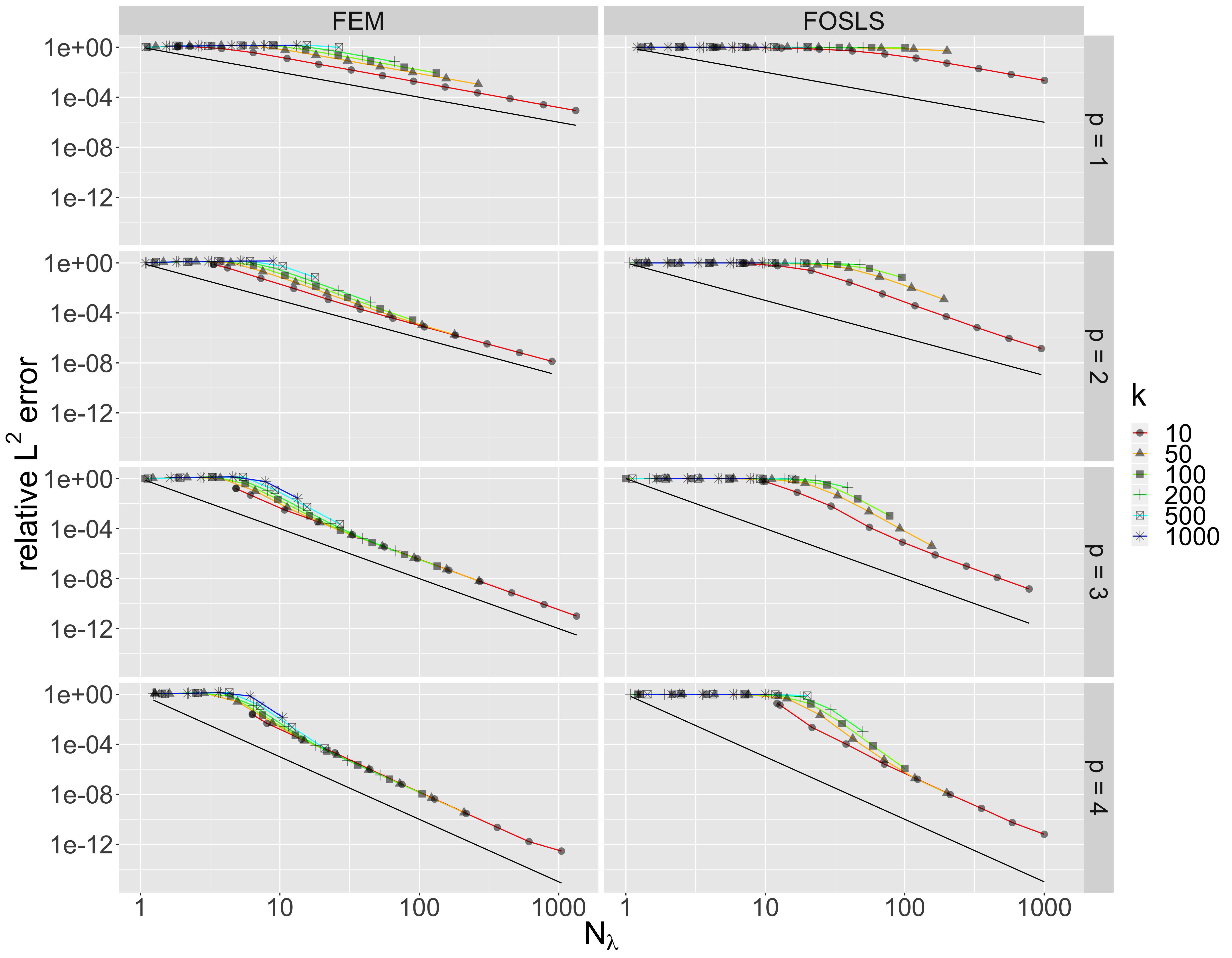
Figure 1: Comparison between the $h$-FEM (left) and $h$-FOSLS (right) for $p=1$, $2$, $3$, $4$ as described in Example 1. The reference line in black corresponds to $h^{p+1}$.

Example 2

For $\pi<\omega<2\pi$ let $\Omega=\{(r\cos\varphi,r\sin\varphi)\colon r\in(0,1),\varphi\in(0,\omega)\}\subset\mathbb{R}^{2}$ and consider

$$-\Delta u-k^{2}u =0\qquad \text{in }\Omega,$$

$$\partial_{n}u-iku =g \text{on }\partial\Omega.$$

The data $g$ is such that the exact solution is given by $u(x,y)=J_{\alpha}(kr)\cos(\alpha\varphi)$, with $\alpha=3\pi/2$. Standard regularity theory gives $u\in H^{1+\alpha-\varepsilon}(\Omega)$ for every $\varepsilon>0$. In the numerical experiments we keep $kh=5$ and perform a $p$-FEM and a $p$-FOSLS method up to $p=46$ and $p=29$, respectively. The results are visualized in Figure 2. We observe that the FEM has significantly smaller errors than the FOSLS. For a discussion of the expected $L^{2}(\Omega)$-convergence rates of the $p$-FEM, we refer the reader to (jensen-suri92, , Remark after Thm. 3 and Section 3).

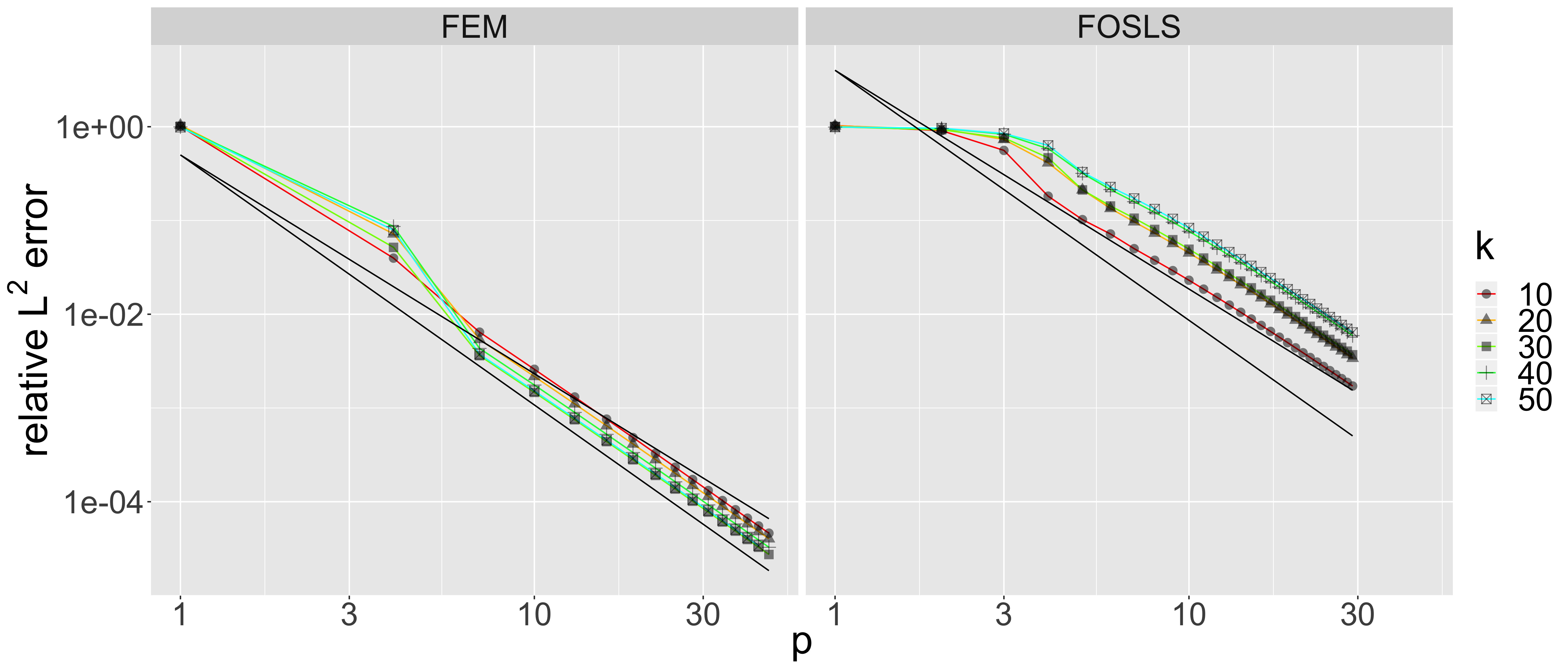
Figure 2: Comparison between the $p$-FEM (left) and $p$-FOSLS (right) for $kh=5$ as described in Example 2. We include the reference lines $p^{-4\cdot 2/3}=p^{-8/3}$ and $p^{-(2\cdot 2/3+1)}=p^{-7/3}$.

The next example focuses on the Helmholtz equation with right-hand side $f$ with finite Sobolev regularity.

Example 3

Let $\Omega=(-1,1)\subset\mathbb{R}$ and $f=-\chi_{(-1,0]}+\chi_{(0,1)}$, where $\chi_{A}$ denotes the indicator function on $A\subset\mathbb{R}$. The function $f$ is in $H^{1/2-\varepsilon}(\Omega)$ for every $\varepsilon>0$. We consider uniform meshes $\mathcal{T}_{h}$ on $\Omega$ such that the break point zero is not a node, as otherwise the piecewise smooth solution could be approximated very well. We study

$$-u^{\prime\prime}-k^{2}u =f\qquad \text{in }\Omega,$$

$$\partial_{n}u-iku =g \text{on }\partial\Omega.$$

where the data $g$ is such that the exact solution is given by

$$u(x)=\begin{cases}\cos(kx)+\frac{1}{k^{2}}&x\leq 0\\ (1+\frac{2}{k^{2}})\cos(kx)-\frac{1}{k^{2}}&x>0\end{cases}$$

Standard regularity theory gives $u\in H^{2.5-\varepsilon}(\Omega)$ for every $\varepsilon>0$. For the $h$-FEM we expect $O(h^{\min(2+0.5,p+1)})$. In fact for $p>1$ one can show (cf. (esterhazy-melenk14, , Cor. 4.6)) that $k\left\lVert u-u_{h}^{\mathrm{FEM}}\right\rVert_{L^{2}(\Omega)}\lesssim h^{2.5}$ and, by inspection, $\left\lVert u\right\rVert_{L^{2}(\Omega)}=O(1)$ (uniformly in $k$). It is therefore expedient to plot $k^{3.5}\left\lVert u-u_{h}^{\mathrm{FEM}}\right\rVert_{L^{2}(\Omega)}/\|u\|_{L^{2}(\Omega)}$ versus $N_{\lambda}\sim(kh)$. For the $h$-FOSLS Corollary 3 predicts only $O(h^{\min(1+0.5,p+1)})$. The numerical results show, however, for both methods convergence $O(h^{\min(2.5,p+1)})$. The results are visualized in Figure 3.

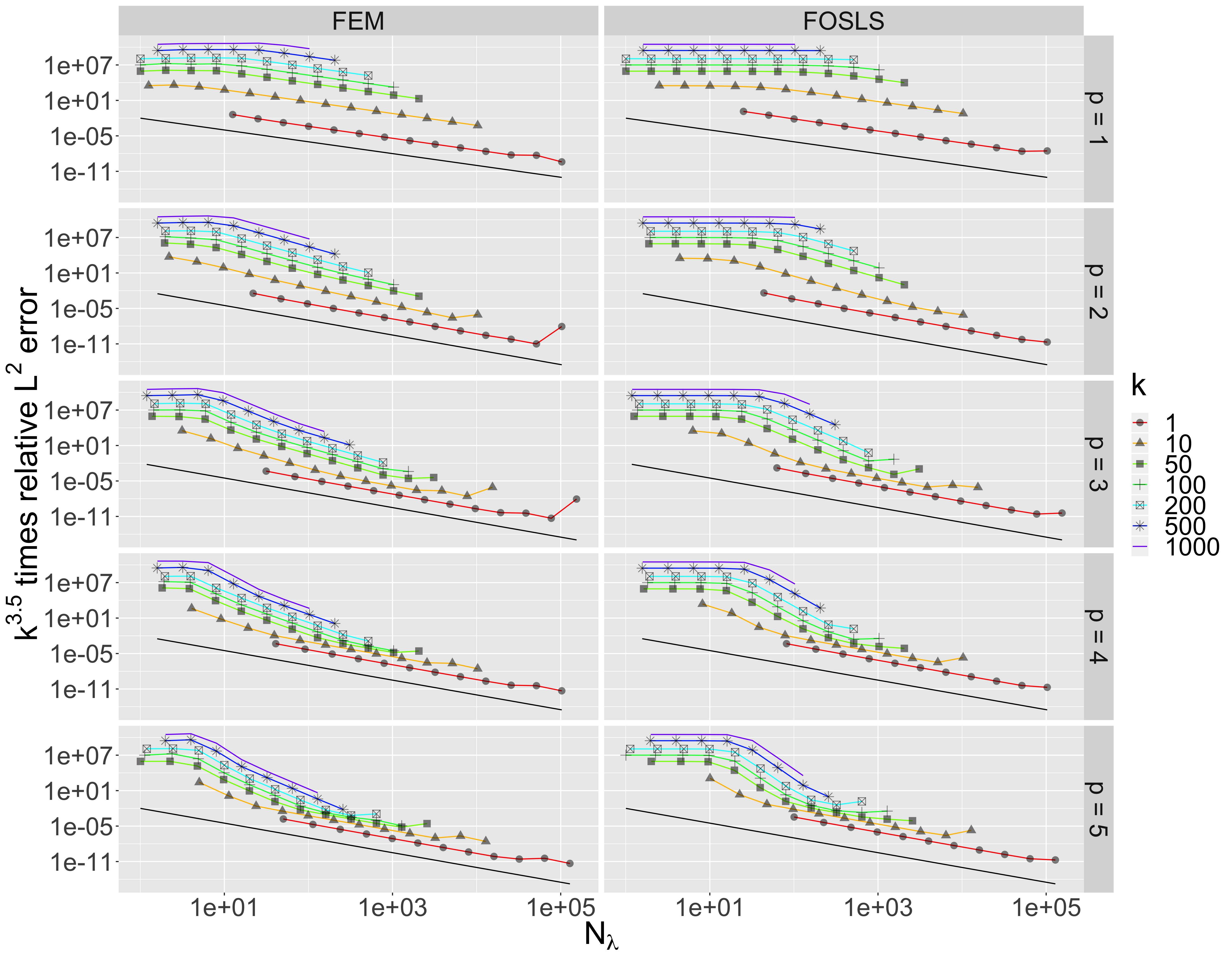
Figure 3: Comparison between the $h$-FEM (left) and $h$-FOSLS (right) for $p=1,\ldots,5$ as described in Example 3. The reference line in black corresponds to $h^{\min(2.5,p+1)}$.

Remark 8

The numerical results of Example 3 visualized in Figure 3 indicate that Corollary 3 is in fact suboptimal as it predicts only a convergence $O(h^{1.5})$ while we observe $O(h^{\min(2.5,p+1)})$. A starting point for understanding this better convergence behavior could be two observations: first, the duality argument in Theorem 5.1 is based on the regularity $(\boldsymbol{\psi},v)\in\boldsymbol{H}^{2}(\Omega)\times H^{2}(\Omega)$ of the dual solution $(\boldsymbol{\psi},v)$ whereas in fact (see the proof of Lemma 1) $(\boldsymbol{\psi},v)\in\boldsymbol{H}^{2}(\operatorname{div},\Omega)\times H^{2}(\Omega)$. Second, a more careful application of the Cauchy-Schwarz inequality (36) at the beginning of the proof of Theorem 5.1 is advisable. In this connection, we point to the fact that the terms in the square brackets in (36) are not of the same order. To illustrate this, we plot the components

$$e_{1}\coloneqq ik\boldsymbol{e^{\varphi}}+\nabla e^{u}\quad\text{ and }\quad e_{2}\coloneqq ike^{u}+\nabla\cdot\boldsymbol{e^{\varphi}}$$ (39)

in Figure 4 for the problem studied in Example 3. ∎

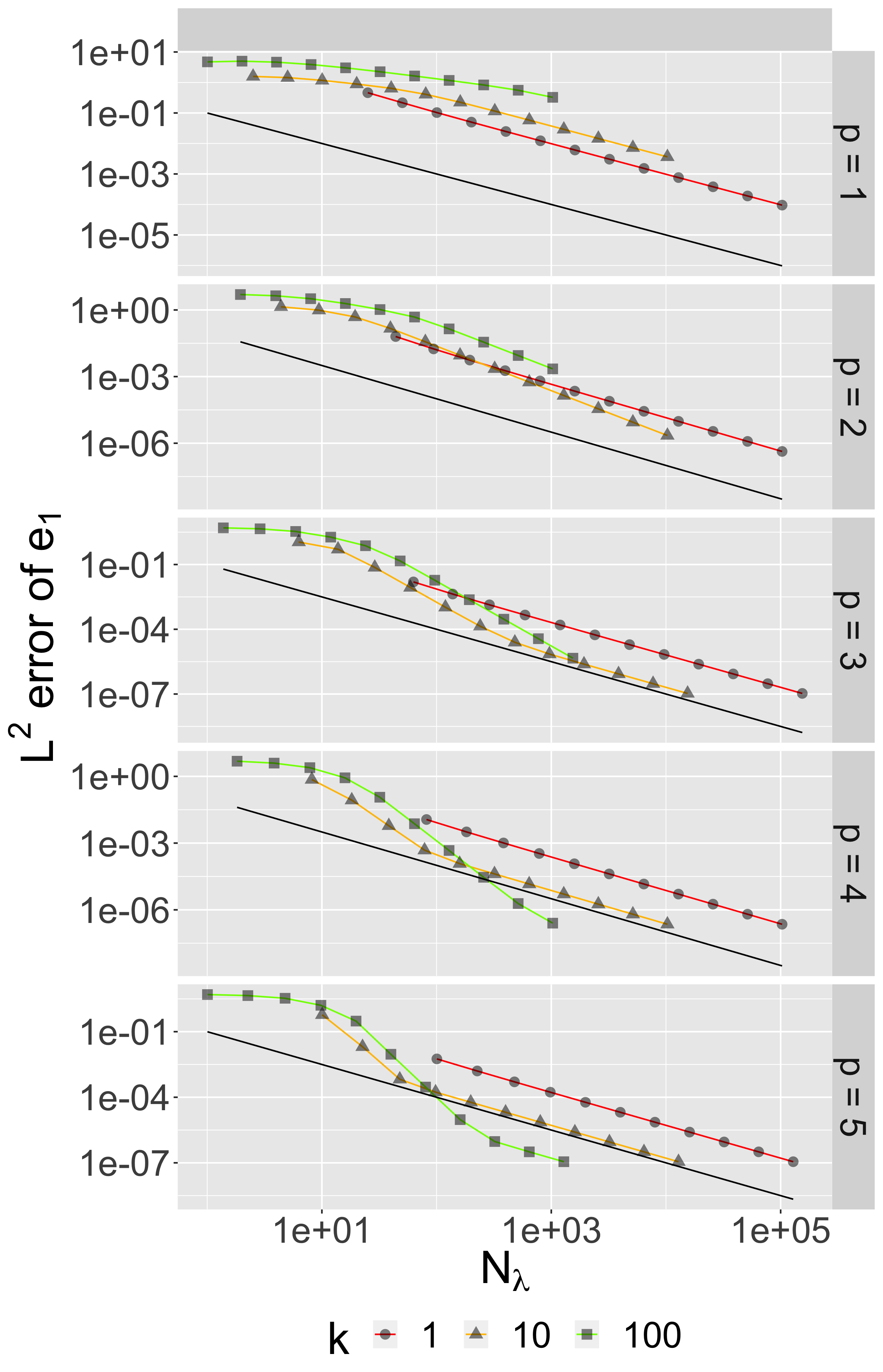
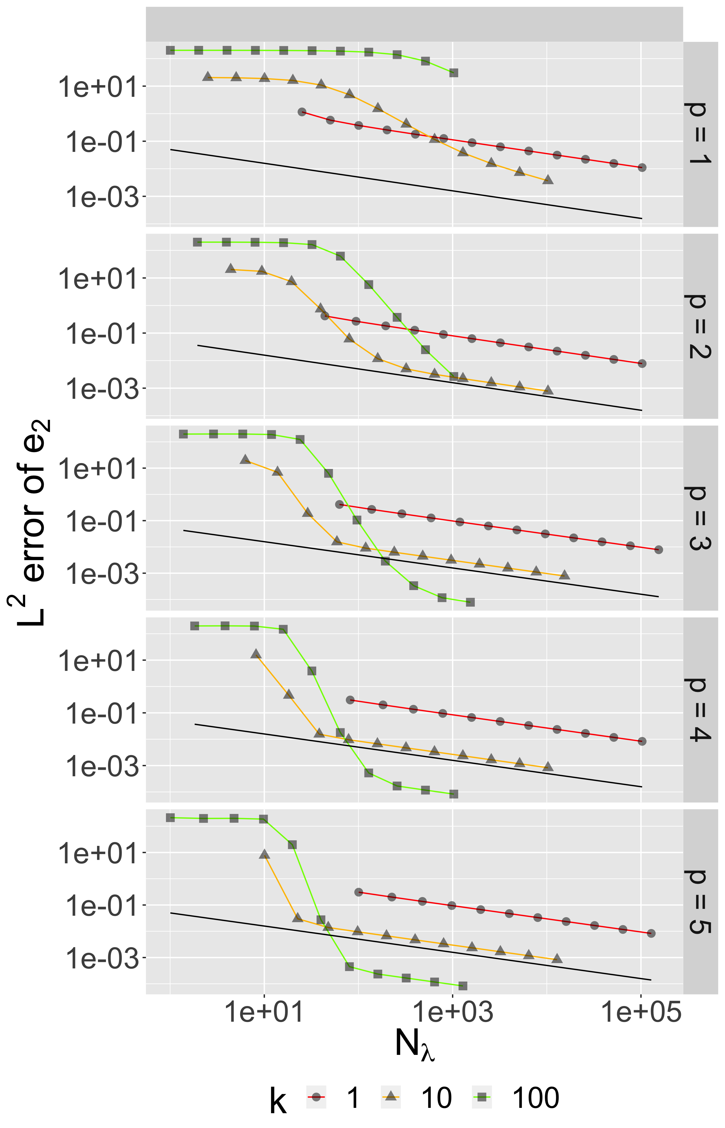
Figure 4: Comparison between the error terms $e_{1}\coloneqq\left\lVert ik\boldsymbol{e^{\varphi}}+\nabla e^{u}\right\rVert_{L^{2}(\Omega)}$ (left) and $e_{2}\coloneqq\left\lVert ike^{u}+\nabla\cdot\boldsymbol{e^{\varphi}}\right\rVert_{L^{2}(\Omega)}$ (right) for $p=1,\ldots,5$ as described in Remark 8 and Example 3. The reference line on the left corresponds to $h^{1}$ for $p=1$ and $h^{1.5}$ for $p>1$. The reference line on the right corresponds to $h^{1/2}$.

Acknowledgement: MB is grateful for the financial support by the Austrian Science Fund (FWF) through the doctoral school Dissipation and dispersion in nonlinear PDEs (grant W1245). MB thanks the workgroup of Joachim Schöberl (TU Wien) for help regarding the numerical experiments.

References

- (1) Ainsworth, M.: Discrete dispersion relation for -version finite element approximation at high wave number. SIAM J. Numer. Anal. 42(2), 553–575 (2004)
- (2) Baskin, D., Spence, E.A., Wunsch, J.: Sharp high-frequency estimates for the Helmholtz equation and applications to boundary integral equations. SIAM J. Math. Anal. 48(1), 229–267 (2016). URL https://doi.org/10.1137/15M102530X
- (3) Chen, H., Lu, P., Xu, X.: A hybridizable discontinuous Galerkin method for the Helmholtz equation with high wave number. SIAM J. Numer. Anal. 51(4), 2166–2188 (2013). URL https://doi.org/10.1137/120883451
- (4) Chen, H., Qiu, W.: A first order system least squares method for the Helmholtz equation. Journal of Computational and Applied Mathematics 309, 145 – 162 (2017). DOI https://doi.org/10.1016/j.cam.2016.06.019. URL http://www.sciencedirect.com/science/article/pii/S0377042716302916
- (5) Demkowicz, L., Gopalakrishnan, J., Muga, I., Zitelli, J.: Wavenumber explicit analysis of a DPG method for the multidimensional Helmholtz equation. Comput. Methods Appl. Mech. Engrg. 213/216, 126–138 (2012). URL https://doi.org/10.1016/j.cma.2011.11.024
- (6) Esterhazy, S., Melenk, J.M.: On stability of discretizations of the Helmholtz equation. In: Numerical analysis of multiscale problems, Lect. Notes Comput. Sci. Eng., vol. 83, pp. 285–324. Springer, Heidelberg (2012). DOI 10.1007/978-3-642-22061-6-9. URL https://doi.org/10.1007/978-3-642-22061-6-9
- (7) Esterhazy, S., Melenk, J.M.: An analysis of discretizations of the Helmholtz equation in and in negative norms. Comput. Math. Appl. 67(4), 830–853 (2014). DOI 10.1016/j.camwa.2013.10.005. URL https://doi.org/10.1016/j.camwa.2013.10.005
- (8) Feng, X., Wu, H.: Discontinuous Galerkin methods for the Helmholtz equation with large wave number. SIAM J. Numer. Anal. 47(4), 2872–2896 (2009). DOI 10.1137/080737538. URL http://dx.doi.org/10.1137/080737538
- (9) Feng, X., Wu, H.: -discontinuous Galerkin methods for the Helmholtz equation with large wave number. Math. Comput. 80, 1997–2024 (2011)
- (10) Feng, X., Xing, Y.: Absolutely stable local discontinuous Galerkin methods for the Helmholtz equation with large wave number. Math. Comp. 82(283), 1269–1296 (2013). URL https://doi.org/10.1090/S0025-5718-2012-02652-4
- (11) Ihlenburg, F.: Finite Element Analysis of Acoustic Scattering, Applied Mathematical Sciences, vol. 132. Springer Verlag (1998)
- (12) Ihlenburg, F., Babuška, I.: Finite element solution to the Helmholtz equation with high wave number. Part I: The -version of the FEM. Comput. Math. Appl. 30, 9–37 (1995)
- (13) Ihlenburg, F., Babuška, I.: Finite element solution to the Helmholtz equation with high wave number. Part II: The -version of the FEM. SIAM J. Numer. Anal. 34, 315–358 (1997)
- (14) Jensen, S., Suri, M.: On the l2 error for the p-version of the finite element method over polygonal domains. Comput. Methods Appl. Mech. Eng. 97(2), 233–243 (1992). DOI 10.1016/0045-7825(92)90165-G. URL http://dx.doi.org/10.1016/0045-7825(92)90165-G
- (15) Lee, B., Manteuffel, T.A., McCormick, S.F., Ruge, J.: First-order system least-squares for the Helmholtz equation. SIAM J. Sci. Comput. 21(5), 1927–1949 (2000). DOI 10.1137/S1064827598339773. URL https://doi.org/10.1137/S1064827598339773. Iterative methods for solving systems of algebraic equations (Copper Mountain, CO, 1998)
- (16) Melenk, J.M.: -finite element methods for singular perturbations, Lecture Notes in Mathematics, vol. 1796. Springer-Verlag, Berlin (2002). URL https://doi.org/10.1007/b84212
- (17) Melenk, J.M.: On approximation in meshless methods. In: Frontiers of numerical analysis, Universitext, pp. 65–141. Springer, Berlin (2005). URL https://doi.org/10.1007/3-540-28884-82
- (18) Melenk, J.M., Parsania, A., Sauter, S.: General dg-methods for highly indefinite helmholtz problems. Journal of Scientific Computing 57(3), 536–581 (2013). DOI 10.1007/s10915-013-9726-8. URL https://doi.org/10.1007/s10915-013-9726-8
- (19) Melenk, J.M., Rojik, C.: On commuting -version projection-based interpolation on tetrahedra (2018). URL https://arxiv.org/abs/1802.00197
- (20) Melenk, J.M., Sauter, S.: Convergence analysis for finite element discretizations of the Helmholtz equation with Dirichlet-to-Neumann boundary conditions. Math. Comp. 79(272), 1871–1914 (2010). URL https://doi.org/10.1090/S0025-5718-10-02362-8
- (21) Melenk, J.M., Sauter, S.: Wavenumber explicit convergence analysis for Galerkin discretizations of the Helmholtz equation. SIAM J. Numer. Anal. 49(3), 1210–1243 (2011). DOI 10.1137/090776202. URL https://doi.org/10.1137/090776202
- (22) Melenk, J.M., Sauter, S.: Wavenumber-explicit -fem analysis for maxwell’s equations with transparent boundary conditions (2018). URL https://arxiv.org/abs/1803.01619
- (23) Monk, P.: Finite element methods for Maxwell’s equations. Numerical Mathematics and Scientific Computation. Oxford University Press, New York (2003). URL https://doi.org/10.1093/acprof:oso/9780198508885.001.0001
- (24) Petrides, S., Demkowicz, L.F.: An adaptive DPG method for high frequency time-harmonic wave propagation problems. Comput. Math. Appl. 74(8), 1999–2017 (2017). URL https://doi.org/10.1016/j.camwa.2017.06.044
- (25) Schöberl, J.: Finite Element Software NETGEN/NGSolve version 6.2. https://ngsolve.org/
- (26) Schöberl, J.: NETGEN - An advancing front 2D/3D-mesh generator based on abstract rules. Computing and Visualization in Science 1(1), 41–52 (1997). DOI 10.1007/s007910050004. URL https://doi.org/10.1007/s007910050004
- (27) Schwab, C.: P- and Hp- Finite Element Methods: Theory and Applications in Solid and Fluid Mechanics. G.H.Golub and others. Clarendon Press (1998)
- (28) Zhu, L., Wu, H.: Preasymptotic error analysis of CIP-FEM and FEM for Helmholtz equation with high wave number. Part II: version. SIAM J. Numer. Anal. 51(3), 1828–1852 (2013). DOI 10.1137/120874643. URL https://doi.org/10.1137/120874643