Sharp ill-posedness of the Dirac-Klein-Gordon system in one dimension

Abstract.

We show the ill-posedness of the Cauchy problem for the Dirac-Klein-Gordon system in one dimension in the critical Sobolev space. From this, we finish the classification of the regularities for which this problem is well-posed or ill-posed.

1. Introduction

We consider the Cauchy problem for the Dirac-Klein-Gordon system:

(1.1) $$\left\{\begin{aligned} &(i\gamma_{0}\partial_{t}+\gamma_{1}\partial_{x})\psi+m\psi=\phi\psi,\\ &(\partial_{t}^{2}-\partial_{x}^{2}+M^{2})\phi=\psi^{\ast}\gamma^{0}\psi,\\ &\psi(0,x)=\psi_{0}(x),\ \phi(0,x)=\phi_{0}(x),\ \partial_{t}\phi(0,x)=\phi_{1}(x),\end{aligned}\right.$$

where $\psi=\bigl{(}\begin{smallmatrix}\psi_{1}\\ \psi_{2}\end{smallmatrix}\bigr{)}:\mathbb{R}^{1+1}\rightarrow\mathbb{C}^{2}$ and $\phi:\mathbb{R}^{1+1}\rightarrow\mathbb{R}$ are unknown functions of $(t,x)\in\mathbb{R}^{1+1}$, $\psi_{0}=\bigl{(}\begin{smallmatrix}\psi_{0,1}\\ \psi_{0,2}\end{smallmatrix}\bigr{)}:\mathbb{R}\rightarrow\mathbb{C}^{2}$ and $\phi_{0},\phi_{1}:\mathbb{R}\rightarrow\mathbb{R}$ are given functions of $x\in\mathbb{R}$. Here, $m$ and $M$ are nonnegative constants, and $\gamma_{0},\gamma_{1}$ are $2\times 2$ Hermitian matrices

(1.2) $$\gamma_{0}=\begin{pmatrix}1&0\\ 0&-1\end{pmatrix},\quad\gamma_{1}=\begin{pmatrix}0&-i\\ i&0\end{pmatrix}$$

which satisfy the anticommutation relations and leads to $(i\gamma_{0}\partial_{t}+\gamma_{1}\partial_{x})^{2}=(-\partial_{t}^{2}+\partial_{x}^{2})I_{2}$ where $I_{2}$ is the $2\times 2$ identity matrix, $\psi^{\ast}$ denotes the conjugate transpose of $\psi$.

We will discuss the well-posedness for the Cauchy problem in (1.1). A problem is called well-posed if a solution exists uniquely and the solution map is continuous. The last property is important in our main theorem in this paper. If the solution map is continuous, the sequence of initial data $u_{n}(0)\to u(0)$ requires the convergence of the corresponding sequence of solutions $u_{n}(t)\to u(t)$ with $t>0$. Here, we are concerned with initial data in the Sobolev spaces $H^{s}(\mathbb{R})$. For $s\in\mathbb{R}$, the Sobolev norm associated with regularity $s$ is given by

$$\|f\|_{H^{s}}=\|\langle\xi\rangle^{s}\hat{f}\|_{L^{2}}=\left(\int_{\mathbb{R}}\langle\xi\rangle^{2s}|\hat{f}(\xi)|^{2}d\xi\right)^{1/2}$$

where $\hat{f}(\xi)=\int_{\mathbb{R}}e^{-ix\xi}f(x)dx$ is the Fourier transform of $f(x)$. We consider the well-posedness in $H^{s}(\mathbb{R})\times H^{r}(\mathbb{R})$ which means

$$(\psi,\phi)\in H^{s}(\mathbb{R})\times H^{r}(\mathbb{R})$$

where we use the symbols $s$ and $r$ for the regularities of $\psi$ and $\phi$ respectively. For brevity, we shall refer to well-posedness from initial data $(\psi_{0},\phi_{0},\phi_{1})\in H^{s}(\mathbb{R})\times H^{r}(\mathbb{R})\times H^{r-1}(\mathbb{R})$ to the solution $(\psi,\phi,\partial_{t}\phi)\in H^{s}(\mathbb{R})\times H^{r}(\mathbb{R})\times H^{r-1}(\mathbb{R})$ as well-posedness in $H^{s}(\mathbb{R})\times H^{r}(\mathbb{R})$.

1.1. Known results

Since we are interested in the classification of well-posedness in this paper, we restrict ourselves to consider the time local issue, namely time local well-posedness or not, and we will not go into the time global issue. If any of the conditions which stipulate well-posedness, namely existence, uniqueness or continuous dependence on the initial data fails, we say that the problem is ill-posed. The first author with Nakanishi and Tsugawa in [16] proved time local well-posedness of (1.1) in the region $|s|\leq r\leq s+1$ except the following forbidden point

(1.3) $$(s,r)=\left(-\frac{1}{2},\frac{1}{2}\right).$$

We call this point the critical point in this paper. In the same paper [16], they proved ill-posedness in the two regions max$\{0,r\}<s$ and max$\{\frac{1}{2},s+1\}<r$. The authors of the current paper proved ill-posedness in the region $s<0,r<\frac{1}{2},s+r<0$ in [19], and on the two lines $s=0,r<0$ and $s<-\frac{1}{2},r=\frac{1}{2}$ in [20]. Thus, well-posedness or ill-posedness of the problem remained open only at the critical point (1.3) (see Figure 1).

Other earlier papers which obtained the well-posedness in subsets of the region $|s|\leq r\leq s+1$ are [2, 3, 4, 6, 7, 8, 9, 10, 15, 22, 23, 24]. There are also global well-posedness results with $s<0$ in which they used Bourgain’s frequency decomposition technique or I-method with a help of the charge conservation law [5, 25, 27].

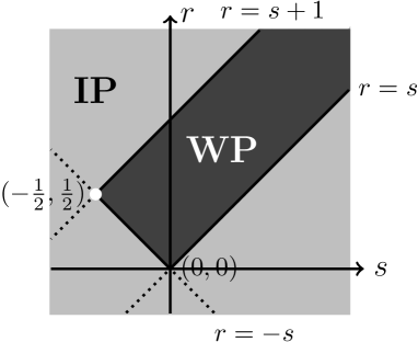
Figure 1. Well-posedness and ill-posedness regions

1.2. Previous attempts at the critcal point

In this subsection, we introduce two partial results connected with well-posedness or ill-posedness at the critical point (1.3). In [16], they proved that the solution map of the Dirac-Klein-Gordon system is not twice differentiable at the origin of $H^{-\frac{1}{2}}(\mathbb{R})\times H^{\frac{1}{2}}(\mathbb{R})$. We remark that the notion of well-posedness does not require twice differentiability for the solution map, and so, this falls slightly short of concluding ill-posedness of the problem.

Shiota in [26] proved that for any initial data $(\psi_{0},\phi_{0},\phi_{1})\in L^{1}(\mathbb{R})\times L^{\infty}(\mathbb{R})\times L^{1}(\mathbb{R})$, there exists a unique solution $(\psi,\phi)\in L^{1}(\mathbb{R})\times L^{\infty}(\mathbb{R})$, and the solution map in this setting is continuous. Even though Shiota has not published his result, there is an introduction to Shiota’s result and proof in the authors’ previous paper [20]. Here we remark the pair of spaces $H^{-\frac{1}{2}}(\mathbb{R})$ and $L^{1}(\mathbb{R})$, and also the pair of $H^{\frac{1}{2}}(\mathbb{R})$ and $L^{\infty}(\mathbb{R})$ share the same scaling property respectively, that is, for $f_{\lambda}(x)=f(\lambda x)$,

$$\frac{\|f_{\lambda}\|_{\dot{H}^{-\frac{1}{2}}}}{\|f_{\lambda}\|_{L^{1}}}=\frac{\|f\|_{\dot{H}^{-\frac{1}{2}}}}{\|f\|_{L^{1}}},\quad\frac{\|f_{\lambda}\|_{\dot{H}^{\frac{1}{2}}}}{\|f_{\lambda}\|_{L^{\infty}}}=\frac{\|f\|_{\dot{H}^{\frac{1}{2}}}}{\|f\|_{L^{\infty}}},\qquad\lambda>0.$$

Since there is no inclusion relation between both pairs $H^{-\frac{1}{2}}(\mathbb{R})$ and $L^{1}(\mathbb{R})$, and $H^{\frac{1}{2}}(\mathbb{R})$ and $L^{\infty}(\mathbb{R})$, this does not lead to the well-posedness of the problem at the critical point.

1.3. Main theorem in this paper

In this paper, we finish the problem. We show ill-posedness at the critical point (1.3) for the problem (1.1). We prove that the solution map of the problem is discontinuous everywhere in $H^{-\frac{1}{2}}(\mathbb{R})\times H^{\frac{1}{2}}(\mathbb{R})\times H^{-\frac{1}{2}}(\mathbb{R})$. Hence this gives a complete classification of the range of Sobolev regularity for well-posedness of (1.1). Those results between the ill-posedness in Sobolev spaces and the well-posedness by Shiota [26] in Lebesgue spaces reminds us the similar situations for the Chern-Simons-Dirac equation in 1d which is ill-posedness by the current authors [19] in Sobolev spaces and well-posedness by the current first author and Ogawa [17] in Lebesgue spaces. Now we state our main theorem.

Theorem 1.1.

For any $\psi_{0}\in H^{-\frac{1}{2}}(\mathbb{R})$, $(\phi_{0},\phi_{1})\in H^{\frac{1}{2}}(\mathbb{R})\times H^{-\frac{1}{2}}(\mathbb{R})$, and any $\varepsilon>0$, there exists a solution $(\psi_{\varepsilon},\phi_{\varepsilon})$ to (1.1) and $t_{\varepsilon}\in(0,\varepsilon)$ such that

$$\|\psi_{\varepsilon}(0)-\psi_{0}\|_{H^{-\frac{1}{2}}}+\|\phi_{\varepsilon}(0)-\phi_{0}\|_{H^{\frac{1}{2}}}+\|\partial_{t}\phi_{\varepsilon}(0)-\phi_{1}\|_{H^{-\frac{1}{2}}}<\varepsilon,$$

$$\|\phi_{\varepsilon}(t_{\varepsilon})\|_{H^{\frac{1}{2}}}>\varepsilon^{-1}.$$

As mentioned in [16] and [20], inconvenient interaction for well-posedness occurs in the nonlinearity $\psi^{\ast}\gamma^{0}\psi$ of the Klein-Gordon equation, and, therefore, we expect that the behavior of $\phi$ gives rise to the ill-posedness. The full details of the proof of Theorem 1.1 are given in the subsequent section, prior to that, we provide an overview of the main ideas. We set some sequence of initial data with parameter $N$ which we will take the limit $N\to\infty$ later. This sequence of initial data converges to 0. We apply an iteration argument, and for that, we write $\phi$ by the series

$$\phi=\sum_{k=1}^{\infty}\phi^{(k)},$$

where $\phi^{(k)}$ is the $k$-th iteration term defined by (2.11) below. The second iteration term is estimated from below with respect to $N$. We show the series converges to the solution of (1.1) by taking the existence time sufficiently small. We show the boundedness of $\phi-\phi^{(2)}$ with respect to $N$. More precisely, we estimate $\phi^{(2)}$ from below by making use of the quadratic interaction of linear solutions of the Dirac equation. We estimate the quadratic interaction, especially of high frequency of those solutions, so this is high $\times$ high $\to$ high type failure of a bilinear estimate. This is different from the abstract argument by Bejenaru-Tao [1], as similar arguments used by Kishimoto-Tsugawa [14] or the authors’ proof for the area $s<0$, $r<\frac{1}{2},s+r<0$ in [19] where they treated high $\times$ high $\to$ low type failure. We can’t apply such abstract theory to obtain the ill-posedness at the critical point (1.3). Our proof is quite straightforward in some sense, that is, an induction argument. We follow the argument by Iwabuchi-Ogawa [12] (see also [13]). We estimate each of the iteration terms, and for then, we make certain delicate estimates for the second iteration term and fortunately, thanks to the smoothing effect of the Duhamel terms, it is enough to roughly estimate the higher order iteration terms.

2. Proof of Theorem 1.1

We will prove Theorem 1.1 under the massless case $m=M=0$ and norm inflation at zero $\psi_{0}=\phi_{0}=\phi_{1}=0$. This is sufficient for the general case in Theorem 1.1 from the argument in [21].

2.1. Preliminaries and iteration setting

Here we introduce the modulation space $M^{0}_{2,1}(\mathbb{R})$, see [11].

Definition 2.1.

Define the space $M^{0}_{2,1}(\mathbb{R})$ as the completion of $C_{0}^{\infty}(\mathbb{R})$ with respect to the norm

$$\|f\|_{M^{0}_{2,1}}=\sum_{k\in\mathbb{Z}}\|\widehat{f}\|_{L^{2}([k-1,k+1])}.$$

The modulation space $M^{0}_{2,1}(\mathbb{R})$ satisfies the embeddings

$$H^{\frac{1}{2}+\varepsilon}(\mathbb{R})\hookrightarrow M^{0}_{2,1}(\mathbb{R})\hookrightarrow L^{2}(\mathbb{R}).$$

Moreover, $M^{0}_{2,1}(\mathbb{R})$ is a Banach algebra, in particular, there exists $C_{1}>1$ such that

(2.1) $$\|fg\|_{M^{0}_{2,1}}\leq C_{1}\|f\|_{M^{0}_{2,1}}\|g\|_{M^{0}_{2,1}}$$

holds true for any $f,g\in M^{0}_{2,1}(\mathbb{R})$.

By setting

$$u:=\psi_{1}-\psi_{2},\quad v:=\psi_{1}+\psi_{2},$$

the system (1.1) with $m=M=0$ is written as follows:

(2.2) $$\begin{cases}(\partial_{t}+\partial_{x})u=-i\phi v,\quad u(0)=u_{0},\\ (\partial_{t}-\partial_{x})v=-i\phi u,\quad v(0)=v_{0},\\ (\partial_{t}^{2}-\partial_{x}^{2})\phi=2\Re(u\bar{v}),\quad\phi(0)=\phi_{0},\ \partial_{t}\phi(0)=\phi_{1},\end{cases}$$

where $\Re z$ is the real part of $z\in\mathbb{C}$. For $N\in{\mathbb{N}}$, we set

(2.3) $$\hat{u}_{0}(\xi)=\sigma_{N}\mathbf{1}_{[5N,7N]}(\xi),$$

(2.4) $$\hat{v}_{0}(\xi)=\sigma_{N}(\log N)^{-\frac{1}{2}}\mathbf{1}_{[-N,0]}(\xi),$$

(2.5) $$\phi_{0}(x)=\phi_{1}(x)=0,$$

where $\sigma_{N}$ converges to zero but slower than $(\log\log N)^{-\frac{1}{2}}$ as $N\to\infty$. Elementary calculations yield

(2.6) $$\|u_{0}\|_{H^{-\frac{1}{2}}} =\sigma_{N}\Big{(}\int_{5N}^{7N}\frac{1}{\langle\xi\rangle}d\xi\Big{)}^{\frac{1}{2}}\sim\sigma_{N},$$

(2.7) $$\|v_{0}\|_{H^{-\frac{1}{2}}} =\sigma_{N}(\log N)^{-\frac{1}{2}}\Big{(}\int_{-N}^{0}\frac{1}{\langle\xi\rangle}d\xi\Big{)}^{\frac{1}{2}}\sim\sigma_{N},$$

(2.8) $$\|\phi_{0}\|_{H^{\frac{1}{2}}} =\|\phi_{1}\|_{H^{-\frac{1}{2}}}=0.$$

Let us define the first iteration

$$u^{(1)}(t,x)=u_{0}(x-t),\quad v^{(1)}(t,x)=v_{0}(x+t),\quad\phi^{(1)}(t,x)=0.$$

For $k\in\mathbb{Z}_{\geq 2}$, we define the higher order iteration functions as follows

(2.9) $$u^{(k)}(t,x) =-i\sum_{\begin{subarray}{c}k_{1},k_{2}\in\mathbb{N}\\ k_{1}+k_{2}=k\end{subarray}}\int_{0}^{t}(\phi^{(k_{1})}v^{(k_{2})})\left(t^{\prime},x-(t-t^{\prime})\right)dt^{\prime},$$

(2.10) $$v^{(k)}(t,x) =-i\sum_{\begin{subarray}{c}k_{1},k_{2}\in\mathbb{N}\\ k_{1}+k_{2}=k\end{subarray}}\int_{0}^{t}(\phi^{(k_{1})}u^{(k_{2})})\left(t^{\prime},x+(t-t^{\prime})\right)dt^{\prime},$$

(2.11) $$\phi^{(k)}(t,x) =2\sum_{\begin{subarray}{c}k_{1},k_{2}\in\mathbb{N}\\ k_{1}+k_{2}=k\end{subarray}}\int_{0}^{t}\frac{\sin(t-t^{\prime})|\partial_{x}|}{|\partial_{x}|}\Re\left(u^{(k_{1})}\overline{v^{(k_{2})}}\right)(t^{\prime},x)dt^{\prime}.$$

We remark here that $\phi^{(1)}=0$ gives

$$u^{(2l)} =v^{(2l)}=\phi^{(2l+1)}=0$$

for any $l\in\mathbb{N}$. We can reduce the number of functions which we need to estimate, but it seems that this does not help the main part of our argument. It still remains to estimate all of the crucial iteration functions.

2.2. Convergence of iteration terms

We shall first show that the following expansions converge in $L^{\infty}([0,T];M^{0}_{2,1}(\mathbb{R}))$ for sufficiently small $T>0$ with fixed $N$,

(2.12) $$u:=\sum_{k=1}^{\infty}u^{(k)},\quad v:=\sum_{k=1}^{\infty}v^{(k)},\quad\phi:=\sum_{k=1}^{\infty}\phi^{(k)},$$

and, moreover, these limits satisfy (2.2). We begin by establishing some precise estimates for $u^{(1)},v^{(1)}$ and $\phi^{(2)}$ in details. We have a constant $C_{2}>1$ such that, for any $t>0$,

(2.13) $$\begin{split}\|u^{(1)}(t)\|_{M^{0}_{2,1}}&=\sum_{k\in\mathbb{Z}}\|e^{it\xi}\hat{u}_{0}\|_{L^{2}[k-1,k+1]}=\sum_{k=5N}^{7N}\|\hat{u}_{0}\|_{L^{2}[k-1,k+1]}\\ &\leq C_{2}\sigma_{N}N,\end{split}$$

and also

$$\begin{split}\|v^{(1)}(t)\|_{M^{0}_{2,1}}&=\sum_{k\in\mathbb{Z}}\|e^{-it\xi}\hat{v}_{0}\|_{L^{2}[k-1,k+1]}=\sum_{k=0}^{N}\|\hat{v}_{0}\|_{L^{2}[k-1,k+1]}\\ &\leq C_{2}\sigma_{N}(\log N)^{-\frac{1}{2}}N.\end{split}$$

Since these estimates are uniform with respect to $t$, we also have

(2.14) $$\|u^{(1)}\|_{L^{\infty}_{t}M^{0}_{2,1}} \leq C_{2}\sigma_{N}N,$$

(2.15) $$\|v^{(1)}\|_{L^{\infty}_{t}M^{0}_{2,1}} \leq C_{2}\sigma_{N}(\log N)^{-\frac{1}{2}}N.$$

We next estimate $\phi^{(2)}$. A direct calculation shows

(2.16) $$\widehat{\phi^{(2)}}(t,\xi)=2\int_{0}^{t}\frac{\sin(t-t^{\prime})\xi}{\xi}\mathcal{F}\left[\Re(u_{0}(x-t^{\prime})\overline{v_{0}(x+t^{\prime})})\right]dt^{\prime}.$$

We calculate the Fourier transform. From $\widehat{\overline{f}}(\xi)=\overline{\widehat{f}}(-\xi)$, we have

$$\mathcal{F}\left[u_{0}(x-t^{\prime})\overline{v_{0}(x+t^{\prime})}\right] =(\widehat{u_{0}}(\xi)e^{-it^{\prime}\xi})*(\widehat{\overline{v_{0}}}(\xi)e^{it^{\prime}\xi})=(\widehat{u_{0}}(\xi)e^{-it^{\prime}\xi})*(\overline{\widehat{v_{0}}}(-\xi)e^{it^{\prime}\xi})$$

$$=\int_{\mathbb{R}}\widehat{u_{0}}(\xi-\eta)e^{-it^{\prime}(\xi-\eta)}\overline{\widehat{v_{0}}}(-\eta)e^{it^{\prime}\eta}d\eta,$$

and so

$$2\mathcal{F}\left[\Re(u_{0}(x-t^{\prime})\overline{v_{0}(x+t^{\prime})})\right]=\mathcal{F}\left[u_{0}(x-t^{\prime})\overline{v_{0}(x+t^{\prime})}+\overline{u_{0}(x-t^{\prime})}v_{0}(x+t^{\prime})\right]$$

$$=\int_{\mathbb{R}}\widehat{u_{0}}(\xi-\eta)e^{-it^{\prime}(\xi-\eta)}\overline{\widehat{v_{0}}}(-\eta)e^{it^{\prime}\eta}d\eta+\overline{\int_{\mathbb{R}}\widehat{u_{0}}(-\xi-\eta)e^{-it^{\prime}(-\xi-\eta)}\overline{\widehat{v_{0}}}(-\eta)e^{it^{\prime}\eta}d\eta}$$

$$=\int_{\mathbb{R}}\widehat{u_{0}}(\xi-\eta)e^{-it^{\prime}(\xi-\eta)}\overline{\widehat{v_{0}}}(-\eta)e^{it^{\prime}\eta}d\eta+\int_{\mathbb{R}}\overline{\widehat{u_{0}}}(-\xi-\eta)e^{-it^{\prime}(\xi+\eta)}\widehat{v_{0}}(-\eta)e^{-it^{\prime}\eta}d\eta.$$

Substituting into (2.16), we get two terms, the first of which is

(2.17) $$\begin{split}&\int_{0}^{t}\frac{\sin(t-t^{\prime})\xi}{\xi}\int_{\mathbb{R}}\widehat{u_{0}}(\xi-\eta)e^{-it^{\prime}(\xi-\eta)}\overline{\widehat{v_{0}}}(-\eta)e^{it^{\prime}\eta}d\eta dt^{\prime}\\ &=\int_{\mathbb{R}}\widehat{u_{0}}(\xi-\eta)\overline{\widehat{v_{0}}}(-\eta)\int_{0}^{t}\frac{e^{it\xi}e^{2it^{\prime}(-\xi+\eta)}-e^{-it\xi}e^{2it^{\prime}\eta}}{2i\xi}dt^{\prime}d\eta\\ &=\frac{1}{4\xi}\int_{\mathbb{R}}\left(e^{it\xi}\frac{e^{2it(\eta-\xi)}-1}{\xi-\eta}+e^{-it\xi}\frac{e^{2it\eta}-1}{\eta}\right)\widehat{u_{0}}(\xi-\eta)\overline{\widehat{v_{0}}}(-\eta)d\eta,\end{split}$$

and the second of which is

(2.18) $$\begin{split}&\int_{0}^{t}\frac{\sin(t-t^{\prime})\xi}{\xi}\int_{\mathbb{R}}\overline{\widehat{u_{0}}}(-\xi-\eta)e^{-it^{\prime}(\xi+\eta)}{\widehat{v_{0}}}(-\eta)e^{-it^{\prime}\eta}d\eta dt^{\prime}\\ &=\frac{1}{4\xi}\int_{\mathbb{R}}\left(e^{it\xi}\frac{e^{-2it(\xi+\eta)}-1}{\xi+\eta}-e^{-it\xi}\frac{e^{-2it\eta}-1}{\eta}\right)\overline{\widehat{u_{0}}}(-\xi-\eta){\widehat{v_{0}}}(-\eta)d\eta.\end{split}$$

From here we consider these terms with the sequence of initial data (2.3) and (2.4) for $\hat{u}_{0}$ and $\hat{v}_{0}$ respectively. Since these are real-valued functions, the complex conjugate disappear. The first term on the right-hand side of (2.17) is estimated as follows:

(2.19) $$\left|\frac{1}{\xi}\int_{\mathbb{R}}e^{it\xi}\frac{e^{2it(\eta-\xi)}-1}{\xi-\eta}\widehat{u_{0}}(\xi-\eta)\widehat{v_{0}}(-\eta)d\eta\right|\leq\sigma_{N}^{2}(\log N)^{-\frac{1}{2}}\frac{\bm{1}_{[5N,8N]}(\xi)}{\xi}.$$

For the second term in (2.17), we change the variable $\eta$ by $\eta/t$ and estimate

(2.20) $$\begin{split}&\left|\frac{1}{\xi}\int_{\mathbb{R}}e^{-it\xi}\frac{e^{2it\eta}-1}{\eta}\widehat{u_{0}}(\xi-\eta)\widehat{v_{0}}(-\eta)d\eta\right|\\ &\leq\sigma_{N}^{2}(\log N)^{-\frac{1}{2}}\int_{0}^{tN}\left|\frac{e^{2i\eta}-1}{\eta}\right|d\eta\ \frac{\bm{1}_{[5N,8N]}(\xi)}{\xi}\\ &\leq\sigma_{N}^{2}(\log N)^{-\frac{1}{2}}(2+\log tN)\ \frac{\bm{1}_{[5N,8N]}(\xi)}{\xi}\end{split}$$

for $tN\geq 1$. The estimate for (2.18) is similar but the support of the corresponding characteristic function is in $[-8N,-5N]$. In total, we obtain

$$|\widehat{\phi^{(2)}}(t,\xi)|\leq 2\sigma_{N}^{2}(\log tN)(\log N)^{-\frac{1}{2}}\frac{\bm{1}_{[5N,8N]}(\xi)+\bm{1}_{[-8N,-5N]}(\xi)}{\xi},$$

provided that $tN\gg 1$. Therefore, from

$$\left\|\mathcal{F}^{-1}\left(\frac{\bm{1}_{[5N,8N]}(\xi)+\bm{1}_{[-8N,-5N]}(\xi)}{\xi}\right)\right\|_{M^{0}_{2,1}}\sim\frac{8N-5N}{N}\sim 1,$$

we have

(2.21) $$\|\phi^{(2)}\|_{L^{\infty}_{t}M^{0}_{2,1}} \leq C_{3}\sigma_{N}^{2}(\log tN)(\log N)^{-\frac{1}{2}}.$$

We now set the time $t=t(N)$ as follows

$$t=N^{-1}(\log N)^{(\log N)^{\frac{1}{2}}}.$$

We enumerate properties of the terms for large $N$ which we will use below: As $N\to\infty$, then $t\to 0$ and

(2.22) $$tN =(\log N)^{(\log N)^{\frac{1}{2}}}\to\infty,$$

(2.23) $$\log(tN) =(\log N)^{\frac{1}{2}}\log\log N\to\infty,$$

(2.24) $$t^{3}N^{2} =N^{-1}(\log N)^{3(\log N)^{\frac{1}{2}}}\to 0,$$

(2.25) $$t^{3}N^{\frac{5}{2}} =N^{-\frac{1}{2}}(\log N)^{3(\log N)^{\frac{1}{2}}}\to 0.$$

To estimate the higher order iteration terms, we use the following lemma ([13], see also Lemma 4.2 in [19]):

Lemma 2.2.

Let $\{a_{n}\}$ be a positive sequence. Assume

(2.26) $$a_{n}\leq C\sum_{\begin{subarray}{c}n_{1},n_{2}\in\mathbb{N},\\ n_{1}+n_{2}=n\end{subarray}}a_{n_{1}}a_{n_{2}}$$

holds. Then, we have

$$a_{n}\leq\left(\frac{2}{3}\pi^{2}C\right)^{n-1}a_{1}^{n}.$$

Lemma 2.3.

There exists a constant $C>1$ such that for any $l\in\mathbb{N}$ and $t\gg N^{-1}$ the following estimates hold:

$$\|\phi^{(2l)}\|_{L^{\infty}_{t}M^{0}_{2,1}} \leq\sigma_{N}^{2l}(\log tN)(\log N)^{-\frac{1}{2}}\left(Ct^{3}N^{2}\right)^{l-1},$$

$$\|u^{(2l+1)}\|_{L^{\infty}_{t}M^{0}_{2,1}} \leq\sigma_{N}^{2l+1}(\log tN)(\log N)^{-1}tN\left(Ct^{3}N^{2}\right)^{l-1},$$

$$\|v^{(2l+1)}\|_{L^{\infty}_{t}M^{0}_{2,1}} \leq\sigma_{N}^{2l+1}(\log tN)(\log N)^{-\frac{1}{2}}tN\left(Ct^{3}N^{2}\right)^{l-1}.$$

Proof.

Let $\{a_{k}\}$ be the sequence defined by

$$a_{1}=\max(C_{2},C_{3}),\quad a_{k}:=2C_{1}\sum_{\begin{subarray}{c}k_{1},k_{2}\in\mathbb{N}\\ k_{1}+k_{2}=k\end{subarray}}a_{k_{1}}a_{k_{2}}$$

for $k\geq 2$, where $C_{1},C_{2}$ and $C_{3}$ are the constants appearing in (2.1), (2.13) and (2.21) respectively. From Lemma 2.2, it suffices to show that

(2.27) $$\|\phi^{(2l)}\|_{L^{\infty}_{t}M^{0}_{2,1}} \leq a_{2l}\sigma_{N}^{2l}(\log tN)(\log N)^{-\frac{1}{2}}\left(t^{3}N^{2}\right)^{l-1},$$

(2.28) $$\|u^{(2l+1)}\|_{L^{\infty}_{t}M^{0}_{2,1}} \leq a_{2l+1}\sigma_{N}^{2l+1}(\log tN)(\log N)^{-1}tN\left(t^{3}N^{2}\right)^{l-1},$$

(2.29) $$\|v^{(2l+1)}\|_{L^{\infty}_{t}M^{0}_{2,1}} \leq a_{2l+1}\sigma_{N}^{2l+1}(\log tN)(\log N)^{-\frac{1}{2}}tN\left(t^{3}N^{2}\right)^{l-1}.$$

We use an induction argument to obtain these estimates. We have done the estimate for $\phi^{(2)}$ in (2.21) which is (2.27) with $l=1$. By (2.11), we have

$$\|\phi^{(2l)}(t)\|_{M^{0}_{2,1}} \leq 2\sum_{\begin{subarray}{c}k_{1},k_{2}\in\mathbb{N}\\ k_{1}+k_{2}=2l\end{subarray}}\int_{0}^{t}(t-t^{\prime})\|u^{(k_{1})}\overline{v^{(k_{2})}}(t^{\prime})\|_{M^{0}_{2,1}}dt^{\prime}$$

$$\leq\sum_{\begin{subarray}{c}k_{1},k_{2}\in\mathbb{N}\\ k_{1}+k_{2}=2l\end{subarray}}C_{1}t^{2}\|u^{(k_{1})}\|_{L^{\infty}_{t}M^{0}_{2,1}}\|{v^{(k_{2})}}\|_{L^{\infty}_{t}M^{0}_{2,1}}.$$

Therefore

(2.30) $$\|\phi^{(2l)}\|_{L^{\infty}_{t}M^{0}_{2,1}} \leq C_{1}t^{2}\sum_{\begin{subarray}{c}k_{1},k_{2}\in\mathbb{N}\\ k_{1}+k_{2}=2l\end{subarray}}\|u^{(k_{1})}\|_{L^{\infty}_{t}M^{0}_{2,1}}\|{v^{(k_{2})}}\|_{L^{\infty}_{t}M^{0}_{2,1}}.$$

Similarly, by (2.9) and (2.10), we have

(2.31) $$\|u^{(2l+1)}\|_{L^{\infty}_{t}M^{0}_{2,1}} \leq C_{1}t\sum_{\begin{subarray}{c}k_{1},k_{2}\in\mathbb{N}\\ k_{1}+k_{2}=2l+1\end{subarray}}\|\phi^{(k_{1})}\|_{L^{\infty}_{t}M^{0}_{2,1}}\|{v^{(k_{2})}}\|_{L^{\infty}_{t}M^{0}_{2,1}},$$

(2.32) $$\|v^{(2l+1)}\|_{L^{\infty}_{t}M^{0}_{2,1}} \leq C_{1}t\sum_{\begin{subarray}{c}k_{1},k_{2}\in\mathbb{N}\\ k_{1}+k_{2}=2l+1\end{subarray}}\|\phi^{(k_{1})}\|_{L^{\infty}_{t}M^{0}_{2,1}}\|{v^{(k_{2})}}\|_{L^{\infty}_{t}M^{0}_{2,1}}.$$

We apply an induction argument with (2.14), (2.15), (2.27), (2.28) and (2.29). So we treat with $u^{(1)},v^{(1)}$ and others differently. Suppose that the estimates (2.27)–(2.29) hold up to some $l\in\mathbb{N}$. Then, from (2.30), we have for large $N$,

$$\|\phi^{(2l+2)}\|_{L^{\infty}M^{0}_{2,1}}$$

$$\leq C_{1}t^{2}\Bigg{\{}\|u^{(2l+1)}\|_{L^{\infty}_{t}M^{0}_{2,1}}\|{v^{(1)}}\|_{L^{\infty}M^{0}_{2,1}}+\|u^{(1)}\|_{L^{\infty}_{t}M^{0}_{2,1}}\|v^{(2l+1)}\|_{L^{\infty}_{t}M^{0}_{2,1}}$$

$$\hskip 80.0pt+\sum_{\begin{subarray}{c}l_{1},l_{2}\in\mathbb{N}\\ l_{1}+l_{2}=l\end{subarray}}\|u^{(2l_{1}+1)}\|_{L^{\infty}_{t}M^{0}_{2,1}}\|v^{(2l_{2}+1)}\|_{L^{\infty}M^{0}_{2,1}}\Bigg{\}}$$

$$\leq C_{1}a_{2l+1}a_{1}\sigma_{N}^{2l+2}(\log tN)(\log N)^{-\frac{3}{2}}(t^{3}N^{2})^{l}$$

$$\qquad+C_{1}a_{1}a_{2l+1}\sigma_{N}^{2l+2}(\log tN)(\log N)^{-\frac{1}{2}}(t^{3}N^{2})^{l}$$

$$\hskip 30.0pt+C_{1}\sum_{\begin{subarray}{c}l_{1},l_{2}\in\mathbb{N}\\ l_{1}+l_{2}=l\end{subarray}}a_{2l_{1}+1}a_{2l_{2}+1}\sigma_{N}^{2l+2}(\log tN)^{2}(\log N)^{-\frac{3}{2}}(tN)^{-2}(t^{3}N^{2})^{l}$$

$$\leq a_{2l+2}\sigma_{N}^{2l+2}(\log tN)(\log N)^{-\frac{1}{2}}(t^{3}N^{2})^{l}.$$

Similarly, for large $N$, we use (2.31)

$$\|u^{(2l+3)}\|_{L^{\infty}_{t}M^{0}_{2,1}}$$

$$\leq C_{1}t\Bigg{\{}\|\phi^{(2l+2)}\|_{L^{\infty}_{t}M^{0}_{2,1}}\|v^{(1)}\|_{L^{\infty}_{t}M^{0}_{2,1}}+\sum_{\begin{subarray}{c}l_{1},l_{2}\in\mathbb{N}\\ l_{1}+l_{2}=l+1\end{subarray}}\|\phi^{(2l_{1})}\|_{L^{\infty}_{t}M^{0}_{2,1}}\|v^{(2l_{2}+1)}\|_{M^{0}_{2,1}}\Bigg{\}}$$

$$\leq C_{1}a_{2l+2}a_{1}\sigma_{N}^{2l+3}(\log tN)(\log N)^{-1}tN(t^{3}N^{2})^{l}$$

$$\hskip 30.0pt+C_{1}\sum_{\begin{subarray}{c}l_{1},l_{2}\in\mathbb{N}\\ l_{1}+l_{2}=l+1\end{subarray}}a_{2l_{1}}a_{2l_{2}+1}\sigma_{N}^{2l+3}(\log tN)^{2}(\log N)^{-1}(tN)^{-1}(t^{3}N^{2})^{l}$$

$$\leq a_{2l+3}\sigma_{N}^{2l+3}(\log tN)(\log N)^{-1}tN(t^{3}N^{2})^{l},$$

and use (2.32) to have

$$\|v^{(2l+3)}\|_{L^{\infty}_{t}M^{0}_{2,1}}$$

$$\leq C_{1}t\Bigg{\{}\|\phi^{(2l+2)}\|_{L^{\infty}_{t}M^{0}_{2,1}}\|u^{(1)}\|_{L^{\infty}_{t}M^{0}_{2,1}}+\sum_{\begin{subarray}{c}l_{1},l_{2}\in\mathbb{N}\\ l_{1}+l_{2}=l+1\end{subarray}}\|\phi^{(2l_{1})}\|_{L^{\infty}_{t}M^{0}_{2,1}}\|u^{(2l_{2}+1)}\|_{L^{\infty}_{t}M^{0}_{2,1}}\Bigg{\}}$$

$$\leq C_{1}a_{2l+2}a_{1}\sigma_{N}^{2l+3}(\log tN)(\log N)^{-\frac{1}{2}}tN(t^{3}N^{2})^{l}$$

$$\hskip 30.0pt+C_{1}\sum_{\begin{subarray}{c}l_{1},l_{2}\in\mathbb{N}\\ l_{1}+l_{2}=l+1\end{subarray}}a_{2l_{1}}a_{2l_{2}+1}\sigma_{N}^{2l+3}(\log tN)^{2}(\log N)^{-\frac{3}{2}}(tN)^{-1}(t^{3}N^{2})^{l}$$

$$\leq a_{2l+3}\sigma_{N}^{2l+3}(\log tN)(\log N)^{-\frac{1}{2}}tN(t^{3}N^{2})^{l}.$$

Therefore, the estimates (2.27)–(2.29) hold true. ∎

This lemma says that the series (2.12) converges in $L^{\infty}([0,T];M^{0}_{2,1}(\mathbb{R}))$ provided that $T^{3}N^{2}<1$ which is satisfied for large $N$ from (2.24). Moreover, since we have a condition on the support of the iteration functions, we estimate the Sobolev norm with respect to the $x$ variable as follows

$$\begin{split}\|\phi^{(2l)}(t)\|_{H^{\frac{1}{2}}}&=\|\mathcal{F}^{-1}[\bm{1}_{[-100^{l}N,100^{l}N]}]\ast\phi^{(2l)}(t)\|_{H^{\frac{1}{2}}}\\ &\lesssim 100^{l}N^{\frac{1}{2}}\|\phi^{(2l)}(t)\|_{M^{0}_{2,1}}\\ &\lesssim\sigma_{N}^{2l}(\log tN)(\log N)^{-1/2}N^{\frac{1}{2}}(100Ct^{3}N^{2})^{l-1}.\end{split}$$

Then the same limit $\phi=\sum_{k=1}^{\infty}\phi^{(k)}$ in the modulation space $M^{0}_{2,1}$ as above also exists in $L^{\infty}([0,T];H^{\frac{1}{2}}(\mathbb{R}))$ provided that $100CT^{3}N^{2}<1$. Moreover if we take $100CT^{3}N^{\frac{5}{2}}<1$ we will have an extra $N^{-\frac{l-1}{2}}$ factor and estimate for each $l\geq 2$

$$\|\phi^{(2l)}(t)\|_{H^{\frac{1}{2}}} \lesssim\sigma_{N}^{2l}(\log tN)(\log N)^{-1/2}N^{\frac{1}{2}}N^{-\frac{l-1}{2}}(100Ct^{3}N^{\frac{5}{2}})^{l-1}$$

$$\lesssim\sigma_{N}^{2l}(\log tN)(\log N)^{-1/2}(100Ct^{3}N^{\frac{5}{2}})^{l-1}$$

where $l=2$ was the worst case but it holds, and other cases $l\geq 3$ were easier. Under the condition $100CT^{3}N^{\frac{5}{2}}<1$ which holds from (2.25), we have

(2.33) $$\sum_{l=2}^{\infty}\|\phi^{(2l)}\|_{L^{\infty}_{T}H^{\frac{1}{2}}}\lesssim\sigma_{N}^{4}(\log tN)(\log N)^{-1/2}.$$

2.3. Lower bound of $\phi^{(2)}$ and conclusion

Here, we establish an appropriate lower bound for $\|\phi^{(2)}(t)\|_{H^{\frac{1}{2}}}$. We decomposed $\widehat{\phi^{(2)}}$ in (2.16) into three terms, (2.18), (2.19) and (2.20). It suffices to establish a lower bound on (2.20) only since (2.18) is negligible if we restrict $\xi\geq 0$ in the norm and we have seen that (2.19) converges to zero faster than (2.20). We write (2.20) here again and estimate

$$\left|\frac{1}{\xi}\int_{\mathbb{R}}e^{-it\xi}\frac{e^{2it\eta}-1}{\eta}\widehat{u_{0}}(\xi-\eta)\widehat{v_{0}}(-\eta)d\eta\right|$$

$$\gtrsim\sigma_{N}^{2}(\log N)^{-1/2}\left|\int_{0}^{N}\frac{e^{2it\eta}-1}{\eta}d\eta\right|\frac{\bm{1}_{[6N,7N]}(\xi)}{|\xi|}$$

$$\gtrsim\sigma_{N}^{2}(\log N)^{-1/2}\log(tN)N^{-1}\bm{1}_{[6N,7N]}(\xi).$$

We obtain

$$\|\phi^{(2)}(t)\|_{H^{\frac{1}{2}}} \geq\left(\int_{0}^{\infty}\langle\xi\rangle|\widehat{\phi^{(2)}}(t,\xi)|^{2}d\xi\right)^{1/2}$$

$$\gtrsim\sigma_{N}^{2}(\log N)^{-1/2}\log(tN)N^{-1}\left(N(7N-6N)\right)^{1/2}$$

$$\sim\sigma_{N}^{2}(\log N)^{-\frac{1}{2}}(\log tN).$$

Therefore, the triangle inequality and Lemma 2.3 with (2.33) yield

(2.34) $$\begin{split}\|\phi(t)\|_{H^{\frac{1}{2}}}&\geq\|\phi^{(2)}(t)\|_{H^{\frac{1}{2}}}-\sum_{l=2}^{\infty}\|\phi^{(2l)}(t)\|_{H^{\frac{1}{2}}}\\ &\gtrsim\sigma_{N}^{2}(\log N)^{-\frac{1}{2}}(\log tN)-\sigma_{N}^{4}(\log N)^{-\frac{1}{2}}(\log tN)\\ &\gtrsim\sigma_{N}^{2}(\log N)^{-\frac{1}{2}}(\log tN)=\sigma_{N}^{2}\log\log N.\end{split}$$

Since $\sigma_{N}$ converges to zero slower than $(\log\log N)^{-\frac{1}{2}}$ as $N\to\infty$, the initial data (2.6), (2.7) and (2.8) converge to zero, still the solution (2.34) is bounded from below. Therefore we conclude the norm inflation for (2.2).

References

- [1] I. Bejenaru and T. Tao, Sharp well-posedness and ill-posedness results for a quadratic non-linear Schrödinger equation, J. Funct. Anal. 233 (2006), no. 1, 228–259.
- [2] N. Bournaveas, A new proof of global existence for the Dirac Klein-Gordon equations in one space dimension, J. Funct. Anal. 173 (2000), no. 1, 203–213.
- [3] N. Bournaveas and D. Gibbeson, Low regularity global solutions of the Dirac-Klein-Gordon equations in one space dimension, Differential Integral Equations 19 (2006), no. 2, 211–222.
- [4] N. Bournaveas and D. Gibbeson, Global charge class solutions of the Dirac-Klein-Gordon equations in one space dimension, Differential Integral Equations 19 (2006), no. 9, 1001–1018.
- [5] T. Candy, Bilinear estimates and applications to global well-posedness for the Dirac-Klein-Gordon equation on , J. Hyperbolic Differ. Equ. 10 (2013), no. 1, 1–35.
- [6] J. Chadam, Global solutions of the Cauchy problem for the (classical) coupled Maxwell-Dirac equations in one space dimension, J. Functional Analysis 13 (1973), 173–184.
- [7] J. Chadam and R. Glassey, On certain global solutions of the Cauchy problem for the (classical) coupled Klein-Gordon-Dirac equations in one and three space dimensions, Arch. Rational Mech. Anal. 54 (1974), 223-237.
- [8] Y. -F. Fang, A direct proof of global existence for the Dirac-Klein-Gordon equations in one space dimension, Taiwanese J. Math. 8 (2004), 33–41.
- [9] Y. -F. Fang, On the Dirac-Klein-Gordon equation in one space dimension, Differential Integral Equations 17 (2004), 1321–1346.
- [10] Y. -F. Fang and H. -C. Huang, A critical case of the Dirac-Klein-Gordon equations in one space dimension, Taiwanese J. Math. 12 (2008), no. 5, 1045–1059.
- [11] H. G. Feichtinger, Modulation spaces on locally compact Abelian groups, Technical Report, University of Vienna, 1983, in: “Proc. Internat. Conf. on Wavelets and Applications” (R. Radha, M. Krishna, and S. Yhangavelu eds.), New Delhi Allied Publishers, (2003), 1–56.
- [12] T. Iwabuchi and T. Ogawa, Ill-posedness for nonlinear Schrödinger equation with quadratic non-linearity in low dimensions, Trans. Amer. Math. Soc. 367 (2015), no. 4, 2613–2630.
- [13] N. Kishimoto, A remark on norm inflation for nonlinear Schrödinger equations, arXiv:1806.10066.
- [14] N. Kishimoto and T. Tsugawa, Local well-posedness for quadratic nonlinear Schrödinger equations and the “good” Bussinesq equation, Differential Integral Equations 23 (2010), no. 5-6, 463–493.
- [15] S. Machihara, The Cauchy problem for the 1-D Dirac–Klein–Gordon equation, NoDEA Nonlinear Differential Equations Appl. 14 (2007), no. 5-6, 625–641.
- [16] S. Machihara, K. Nakanishi, and K. Tsugawa, Well-posedness for nonlinear Dirac equations in one dimension, Kyoto J. Math. 50 (2010), no. 2, 403–451.
- [17] S. Machihara and T. Ogawa, Global wellposedness for a one-dimensional Chern-Simons-Dirac system in , Comm. Partial Differential Equations 42 (2017), no. 8, 1175–1198.
- [18] S. Machihara and M. Okamoto, Ill-posedness of the Cauchy problem for the Chern-Simons-Dirac system in one dimension, J. Differential Equations 258 (2015), 1356-1394.
- [19] S. Machihara and M. Okamoto, Sharp well-posedness and ill-posedness for the Chern-Simons-Dirac system in one dimension, Int. Math. Res. Not. IMRN 2016, no. 6, 1640–1694.
- [20] S. Machihara and M. Okamoto, Remarks on ill-posedness for the Dirac-Klein-Gordon system, Dyn. Partial Differ. Equ. 13 (2016), no. 3, 179–190.
- [21] M. Okamoto Norm inflation for the generalized Boussinesq and Kawahara equations, Nonlinear Anal. 157 (2017), 44–61.
- [22] H. Pecher, Low regularity well-posedness for the one-dimensional Dirac-Klein-Gordon system, Electron. J. Differential Equations (2006), No. 150, 13 pp.
- [23] S. Selberg and A. Tesfahun, Low regularity well-posedness of the Dirac-Klein-Gordon system in one space dimension, Commun. Contemp. Math. 10 (2008), no. 2, 181–194.
- [24] S. Selberg and A. Tesfahun, Remarks on regularity and uniqueness of the Dirac-Klein-Gordon equations in one space dimension, NoDEA Nonlinear Differential Equations Appl. 17 (2010), no. 4, 453–465.
- [25] S. Selberg, Global well-posedness below the charge norm for the Dirac-Klein-Gordon system in one space dimension, Int. Math. Res. Not. IMRN. 17 (2008), Art. ID rnm058, 25 pp.
- [26] R. Shiota, Well-posedness of the Cauchy problem for the one dimensional Dirac-Klein-Gordon system, Master’s Thesis, Saitama University, 2015.
- [27] A. Tesfahun, Global well-posedness of the 1D Dirac-Klein-Gordon system in Sobolev spaces of negative index, J. Hyperbolic Differ. Equ. 6. (2009), no 3, 631–661.