Two-loop effective potential for generalized gauge fixing

Abstract

We obtain the two-loop effective potential for general renormalizable theories, using a generalized gauge-fixing scheme that includes as special cases the background-field $R_{\xi}$ gauges, the Fermi gauges, and the familiar Landau gauge, and using dimensional regularization in the bare and $\overline{\rm{MS}}$ renormalization schemes. As examples, the results are then specialized to the Abelian Higgs model and to the Standard Model. In the case of the Standard Model, we study how the vacuum expectation value and the minimum vacuum energy depend numerically on the gauge-fixing parameters. The results at fixed two-loop order exhibit non-convergent behavior for sufficiently large gauge-fixing parameters; this can presumably be addressed by a resummation of higher-order contributions.

I Introduction

The effective potential Coleman:1973jx ; Jackiw:1974cv ; Sher:1988mj is a useful tool for the quantitative understanding of spontaneous symmetry breaking, with the most obvious application being to electroweak symmetry breaking in the Standard Model and its extensions.

In gauge theories, the effective potential is simplest and easiest to compute in Landau gauge. The 2-loop order effective potential was originally obtained for the Standard Model in Ford:1992pn , and extended to general theories in Martin:2001vx . The leading 3-loop contributions for the Standard Model were obtained in ref. Martin:2013gka in the approximation that the QCD and top-quark Yukawa couplings are treated as much larger than the other dimensionless couplings. These results were then extended to full 3-loop order for a general theory in ref. Martin:2017lqn , where they were written in terms of the basis of 3-loop vacuum integral functions with arbitrary masses, as given in Martin:2016bgz . (For an alternative treatment of the necessary basis integral functions, see Bauberger:2017nct .) When the tree-level Goldstone boson squared mass is small or negative, as indeed occurs in the Standard Model, infrared (IR) divergences or spurious imaginary parts arise in the effective potential, but it has been shown that a resummation of Goldstone boson propagator contributions cures this issue Martin:2014bca ; Elias-Miro:2014pca ; for further development and related perspectives, see Pilaftsis:2015cka ; Pilaftsis:2015bbs ; Kumar:2016ltb ; Braathen:2016cqe ; Pilaftsis:2017enx ; Braathen:2017izn ; Espinosa:2017aew . The 4-loop contributions to the Standard Model effective potential at leading order in QCD are also known Martin:2015eia . One application of these results is to precision calculations of physical masses and other observables in the Standard Model using the tadpole-free scheme, which means that perturbation theory is organized around a vacuum expectation value (VEV) defined as the minimum of the effective potential. This contrasts with the choice of expanding around the minimum of the tree-level potential, which is often done but then requires inclusion of tadpole diagrams and has formally slower convergence properties. Full two-loop electroweak corrections to the Higgs boson, $W$, $Z$, and top-quark masses in this tadpole-free scheme have been give in refs. Martin:2014cxa ; Martin:2015lxa ; Martin:2015rea ; Martin:2016xsp ; these rely on the two-loop Standard Model effective potential result. Softly-broken supersymmetric theories require a different renormalization scheme based on dimensional reduction rather than dimensional regularization, and the 2-loop effective potential for the minimal supersymmetric extension of the Standard Model has been obtained accordingly in refs. Hempfling:1993qq ; Zhang:1998bm ; Espinosa:1999zm ; Espinosa:2000df , Martin:2001vx , Martin:2002iu . All of these multi-loop results have been obtained in Landau gauge and no other, up to now. We think it is reasonable to assert that Landau gauge is the preferred choice whenever the effective potential plays a central role in high precision calculations.

However, it is also sometimes considered beneficial to make use of gauge invariance as a check of both calculations and conceptual understanding. This can be done by considering the effective potential obtained with other gauge-fixing schemes. It has long been understood Jackiw:1974cv ; Dolan:1974gu that the effective potential, and the vacuum expectation values of scalar fields defined by its minimum, does depend on the gauge-fixing choice. This is not a problem, because physical observables following from the effective potential, including its values at local minima, pole masses of particles, and properly defined transition rates, are independent of the choice of gauge fixing. Important results and a variety of perspectives on the issues related to the gauge dependence of the effective potential and the gauge independence of physical observables can be found in Jackiw:1974cv ; Dolan:1974gu ; Kang:1974yj ; Fischler:1974ue ; Frere:1974ia ; Nielsen:1975fs ; Fukuda:1975di ; Aitchison:1983ns ; Metaxas:1995ab ; Loinaz:1997td ; DelCima:1999gg ; Gambino:1999ai ; Alexander:2008hd ; Patel:2011th ; Lewandowski:2013uha ; DiLuzio:2014bua ; Nielsen:2014spa ; Andreassen:2014eha ; Andreassen:2014gha ; Espinosa:2015qea ; Plascencia:2015pga ; Lalak:2016zlv ; Espinosa:2016uaw ; Espinosa:2016nld ; Endo:2017gal ; Irges:2017ztc . The Nielsen identities Nielsen:1975fs ; Fukuda:1975di parameterize the fact that the gauge-fixing dependence of the effective potential can always be absorbed into a redefinition of the scalar fields. However, these identities hold to all orders in perturbation theory, and practical results that are truncated at finite order often require a careful treatment in order to demonstrate gauge-fixing independence of physical quantities. In some cases, there are subtleties involved in verifying that a particular version of a calculated quantity of interest is really a physical observable. Recently, it has been argued that resummations of diagrams to all orders in perturbation theory are necessary to make manifest the gauge-fixing independence Andreassen:2014eha and to cure Espinosa:2016uaw related infrared (IR) divergence problems Aitchison:1983ns ; Loinaz:1997td that occur in Fermi gauges.

One of the uses of the effective potential is to study the stability of the Standard Model vacuum with respect to the Higgs field Lindner:1988ww ; Arnold:1991cv ; Ford:1992mv ; Casas:1994qy ; Espinosa:1995se ; Casas:1996aq , Loinaz:1997td , Isidori:2001bm ; Espinosa:2007qp ; ArkaniHamed:2008ym ; Bezrukov:2009db ; Ellis:2009tp ; EliasMiro:2011aa ; Bezrukov:2012sa ; Degrassi:2012ry ; Alekhin:2012py ; Buttazzo:2013uya , DiLuzio:2014bua ; Espinosa:2015qea ; Espinosa:2016nld , Andreassen:2017rzq ; Chigusa:2017dux . The observed value of the Higgs boson mass near 125 GeV implies that the electroweak vacuum is metastable, if one assumes that the Standard Model holds without extension up to very high energy scales. As noted particularly in Loinaz:1997td ; DiLuzio:2014bua , it is non-trivial to identify an instability scale that is gauge-independent. Care is needed to identify physical observables correlated with the vacuum instability problem, and to ensure that practical calculations of them in perturbation theory maintain the gauge invariance that in principle should govern an all-orders calculation, as dictated by the Nielsen identities.

In this paper, we provide a calculation of the 2-loop effective potential in a general linear gauge-fixing scheme, but leave aside such issues as resummation. We will provide results for a general gauge theory, and then specialize to the Abelian Higgs model and the Standard Model as examples.

To establish notations and conventions, let us write the bosonic degrees of freedom in the Lagrangian as a list of real gauge vector bosons $A^{a}_{\mu}(x)$ and a list of real scalar fields $\Phi_{j}(x)$. The latter transform under the gauge group with generators $t^{a}_{jk}$, which are Hermitian, antisymmetric, and therefore purely imaginary matrices. The indices $j,k,\ldots$ label the real scalars, and $a,b,\ldots$ are adjoint representation indices for the real vector fields $A^{a}_{\mu}$, with coupling constants $g_{a}$ and totally antisymmetric structure constants $f^{abc}$, determined by $[t^{a},t^{b}]=if^{abc}t^{c}$. Before gauge fixing, the Lagrangian is:

$${\cal L}_{\rm YM} = -\frac{1}{4}F^{\mu\nu a}F_{\mu\nu}^{a}-\frac{1}{2}D^{\mu}\Phi_{j}D_{\mu}\Phi_{j}-V(\Phi_{j})+{\cal L}_{\rm fermions},$$ (1.1)

where $V(\Phi_{j})$ is the tree-level scalar potential, and

$$F_{\mu\nu}^{a} = \partial_{\mu}A_{\nu}^{a}-\partial_{\nu}A_{\mu}^{a}+g_{a}f^{abc}A_{\mu}^{b}A_{\nu}^{c},$$ (1.2)

$$D_{\mu}\Phi_{j} = \partial_{\mu}\Phi_{j}-ig_{a}A^{a}_{\mu}t^{a}_{jk}\Phi_{k}.$$ (1.3)

Now we write each real scalar field as the sum of a constant background field $\phi_{j}$ and a dynamical field $R_{j}$,

$$\Phi_{j}(x) = \phi_{j}+R_{j}(x).$$ (1.4)

In this background, the fermion Lagrangian for a general renormalizable theory can be written as

$${\cal L}_{\rm fermions} = i\psi^{\dagger I}\overline{\sigma}^{\mu}D_{\mu}\psi_{I}-\frac{1}{2}(M^{II^{\prime}}\psi_{I}\psi_{I^{\prime}}+Y^{jIJ}R_{j}\psi_{I}\psi_{J}+{\rm c.c.}).$$ (1.5)

Here $\psi_{I}$ are two-component left-handed fermion fields, labeled by capital letters from the middle of the alphabet, $I,J,K,\ldots$. The covariant derivative acting on fermions is

$$D_{\mu}\psi_{I} = \partial_{\mu}\psi_{I}-ig_{a}A^{a}_{\mu}T^{aJ}_{I}\psi_{J},$$ (1.6)

with gauge group generator Hermitian matrices $T^{aJ}_{I}$, which also satisfy $[T^{a},T^{b}]=if^{abc}T^{c}$. In eq. (1.5), $Y^{jIJ}$ are Yukawa couplings, and $M^{II^{\prime}}$ are $\phi_{j}$-dependent fermion masses. It is assumed that (by performing an appropriate unitary rotation on the fermion indices) the fields $\psi_{I}$ have been arranged to be eigenstates of the background field-dependent squared masses

$$M_{I}^{2}=M_{I^{\prime}}^{2}=|M^{II^{\prime}}|^{2},$$ (1.7)

such that the mass matrix $M^{II^{\prime}}$ connects pairs of fermion fields with opposite conserved charges. Thus, it is understood that primed indices $I^{\prime},J^{\prime},K^{\prime}\ldots$ label the mass partners of fermions with the opposite charges labeled $I,J,K,\ldots$ when they form a Dirac pair, while $I^{\prime}=I$ for each fermion with a Majorana mass and no conserved charge left unbroken by the background fields $\phi_{j}$. Because two-component fermion fields are intrinsically complex, the heights of the fermion indices are significant, and raising and lowering them is taken to indicate complex conjugation, so that:

$$M_{II^{\prime}}=(M^{II^{\prime}})^{*};\qquad\quad Y_{jIJ}=(Y^{jIJ})^{*};\qquad\quad T^{aI}_{J}=(T^{aJ}_{I})^{*}.$$ (1.8)

The effective potential is then a function of the constant background fields $\phi_{j}$, and can be evaluated in a loop expansion:

$$V_{\rm eff}(\phi_{j}) = V^{(0)}(\phi_{j})+\frac{1}{16\pi^{2}}V^{(1)}(\phi_{j})+\frac{1}{(16\pi^{2})^{2}}V^{(2)}(\phi_{j})+\ldots,$$ (1.9)

where $V^{(0)}(\phi_{j})=V(\phi_{j})$ is the tree-level part, and the contribution $V^{(n)}$ is obtained for $n\geq 1$ from the sum of 1-particle irreducible $n$-loop Feynman diagrams with no external legs. Carrying out the evaluation of the loop corrections requires gauge fixing and regularization of divergences.

A useful consistency check is obtained from renormalization group invariance of the $\overline{\rm{MS}}$ form of the effective potential. Writing the loop expansion of the beta function for each $\overline{\rm{MS}}$ parameter $X$ (including the background fields $\phi_{j}$, and the gauge-fixing parameters discussed below) as

$$Q\frac{dX}{dQ}\equiv\beta_{X} = \frac{1}{16\pi^{2}}\beta^{(1)}_{X}+\frac{1}{(16\pi^{2})^{2}}\beta^{(2)}_{X}+\ldots,$$ (1.10)

then the requirement

$$Q\frac{dV_{\rm eff}}{dQ}=\Bigl{(}Q\frac{\partial}{\partial Q}+\sum_{X}\beta_{X}\frac{\partial}{\partial X}\Bigr{)}V_{\rm eff} = 0$$ (1.11)

yields

$$Q\frac{\partial}{\partial Q}V^{(\ell)}+\sum_{n=0}^{\ell-1}\Bigl{(}\sum_{X}\beta_{X}^{(\ell-n)}\frac{\partial}{\partial X}V^{(n)}\Bigr{)} = 0$$ (1.12)

at each loop order $\ell=1,2,\ldots$.

II Generalized gauge fixing

To treat the gauge fixing, consider an off-shell BRST BRST formalism for the gauge invariance, with Grassmann-odd ghost and anti-ghost fields $\eta^{a}$ and $\overline{\eta}^{a}$, and bosonic Nakanishi-Lautrup NakanishiLautrup auxiliary fields $b^{a}$. The BRST transformations of the fields are essentially gauge transformations parameterized by the ghost fields $\eta^{a}$:

$$\delta_{\rm BRST}A_{\mu}^{a} = \partial_{\mu}\eta^{a}-g_{a}f^{abc}\eta^{b}A^{c}_{\mu},$$ (2.1)

$$\delta_{\rm BRST}R_{j} = ig_{a}\eta^{a}t^{a}_{jk}(\phi_{k}+R_{k}),$$ (2.2)

$$\delta_{\rm BRST}\psi_{I} = ig_{a}\eta^{a}T^{aJ}_{I}\psi_{I},$$ (2.3)

$$\delta_{\rm BRST}\eta^{a} = -\frac{1}{2}g_{a}f^{abc}\eta^{b}\eta^{c},$$ (2.4)

$$\delta_{\rm BRST}\overline{\eta}^{a} = b^{a},$$ (2.5)

$$\delta_{\rm BRST}b^{a} = 0.$$ (2.6)

From these one can check the nilpotency of the BRST transformations:

$$\delta_{\rm BRST}(\delta_{\rm BRST}X)=0$$ (2.7)

for any field $X$. (Note that $\delta_{\rm BRST}$ is Grassmann-odd; it obtains a minus sign when moved past a fermion or ghost field.) The Lagrangian in eq. (1.1) is invariant under this BRST transformation. Together, these facts mean that we can obtain a BRST-invariant gauge-fixed Lagrangian by:

$${\cal L} = {\cal L}_{\rm YM}+{\cal L}_{\rm g.f.}+{\cal L}_{\rm ghost},$$ (2.8)

where the gauge-fixing plus ghost part is obtained as a BRST variation:

$${\cal L}_{\rm g.f.}+{\cal L}_{\rm ghost} = \delta_{\rm BRST}\Bigl{(}\overline{\eta}^{a}\Bigl{[}\frac{1}{2}\xi_{a}b^{a}-\partial^{\mu}A^{a}_{\mu}-ig_{a}\mathchoice{\accentset{\displaystyle\text{\smash{\raisebox{-5.59721pt}{$\widetildesym$}}}}{\phi}}{\accentset{\textstyle\text{\smash{\raisebox{-5.59721pt}{$\widetildesym$}}}}{\phi}}{\accentset{\scriptstyle\text{\smash{\raisebox{-3.91806pt}{$\widetildesym$}}}}{\phi}}{\accentset{\scriptscriptstyle\text{\smash{\raisebox{-2.7986pt}{$\widetildesym$}}}}{\phi}}_{j}^{a}t^{a}_{jk}R_{k}\Bigr{]}\Bigr{)}.$$ (2.9)

Here $\xi_{a}$ and $\mathchoice{\accentset{\displaystyle\text{\smash{\raisebox{-5.59721pt}{$\widetildesym$}}}}{\phi}}{\accentset{\textstyle\text{\smash{\raisebox{-5.59721pt}{$\widetildesym$}}}}{\phi}}{\accentset{\scriptstyle\text{\smash{\raisebox{-3.91806pt}{$\widetildesym$}}}}{\phi}}{\accentset{\scriptscriptstyle\text{\smash{\raisebox{-2.7986pt}{$\widetildesym$}}}}{\phi}}_{j}^{a}$ are gauge-fixing parameters; in general the latter may or may not be related to the background scalar fields $\phi_{j}$ that the effective potential depends on. It follows that

$${\cal L}_{\rm g.f.} = \frac{1}{2}\xi_{a}b^{a}b^{a}-b^{a}\Bigl{(}\partial^{\mu}A^{a}_{\mu}+ig_{a}\mathchoice{\accentset{\displaystyle\text{\smash{\raisebox{-5.59721pt}{$\widetildesym$}}}}{\phi}}{\accentset{\textstyle\text{\smash{\raisebox{-5.59721pt}{$\widetildesym$}}}}{\phi}}{\accentset{\scriptstyle\text{\smash{\raisebox{-3.91806pt}{$\widetildesym$}}}}{\phi}}{\accentset{\scriptscriptstyle\text{\smash{\raisebox{-2.7986pt}{$\widetildesym$}}}}{\phi}}^{a}_{j}t^{a}_{jk}R_{k}\Bigr{)}$$ (2.10)

and

$${\cal L}_{\rm ghost} = -\partial_{\mu}\overline{\eta}^{a}\partial^{\mu}\eta^{a}+g_{a}f^{abc}\partial^{\mu}\overline{\eta}^{a}\eta^{b}A_{\mu}^{c}+[g_{a}t^{a}_{kj}\mathchoice{\accentset{\displaystyle\text{\smash{\raisebox{-5.59721pt}{$\widetildesym$}}}}{\phi}}{\accentset{\textstyle\text{\smash{\raisebox{-5.59721pt}{$\widetildesym$}}}}{\phi}}{\accentset{\scriptstyle\text{\smash{\raisebox{-3.91806pt}{$\widetildesym$}}}}{\phi}}{\accentset{\scriptscriptstyle\text{\smash{\raisebox{-2.7986pt}{$\widetildesym$}}}}{\phi}}^{a}_{j}][g_{b}t^{b}_{kl}(\phi_{l}+R_{l})]\overline{\eta}^{a}\eta^{b}.$$ (2.11)

By integrating out the auxiliary fields $b^{a}$, one can re-write eq. (2.10) as:

$${\cal L}_{\rm g.f.} = -\frac{1}{2\xi_{a}}\left(\partial^{\mu}A^{a}_{\mu}+ig_{a}\mathchoice{\accentset{\displaystyle\text{\smash{\raisebox{-5.59721pt}{$\widetildesym$}}}}{\phi}}{\accentset{\textstyle\text{\smash{\raisebox{-5.59721pt}{$\widetildesym$}}}}{\phi}}{\accentset{\scriptstyle\text{\smash{\raisebox{-3.91806pt}{$\widetildesym$}}}}{\phi}}{\accentset{\scriptscriptstyle\text{\smash{\raisebox{-2.7986pt}{$\widetildesym$}}}}{\phi}}^{a}_{j}t^{a}_{jk}R_{k}\right)^{2}.$$ (2.12)

There are various special cases of the above general gauge-fixing condition that are of interest:

• Landau gauge:  $\mathchoice{\accentset{\displaystyle\text{\smash{\raisebox{-5.59721pt}{$\widetildesym$}}}}{\phi}}{\accentset{\textstyle\text{\smash{\raisebox{-5.59721pt}{$\widetildesym$}}}}{\phi}}{\accentset{\scriptstyle\text{\smash{\raisebox{-3.91806pt}{$\widetildesym$}}}}{\phi}}{\accentset{\scriptscriptstyle\text{\smash{\raisebox{-2.7986pt}{$\widetildesym$}}}}{\phi}}^{a}_{j}=0$ and $\xi_{a}\rightarrow 0$. This condition is renormalization group invariant, and avoids kinetic mixing between scalar and vector fields. The resulting simplicity is why this gauge condition is by far the most popular one for practical applications involving the effective potential.

• Fermi gauges:  $\mathchoice{\accentset{\displaystyle\text{\smash{\raisebox{-5.59721pt}{$\widetildesym$}}}}{\phi}}{\accentset{\textstyle\text{\smash{\raisebox{-5.59721pt}{$\widetildesym$}}}}{\phi}}{\accentset{\scriptstyle\text{\smash{\raisebox{-3.91806pt}{$\widetildesym$}}}}{\phi}}{\accentset{\scriptscriptstyle\text{\smash{\raisebox{-2.7986pt}{$\widetildesym$}}}}{\phi}}^{a}_{j}=0$. This condition is renormalization group invariant. However, the parameters $\xi_{a}$ do run with the renormalization scale (except when they vanish). A further complication is that when $\xi_{a}\not=0$, the scalar and vector fields have propagator mixing with each other, which arises due to cross-terms $A^{a}_{\mu}\partial^{\mu}R_{j}$ in the scalar kinetic term in eq. (1.1). In the Landau gauge limit $\xi_{a}\rightarrow 0$, the effects of this cross-term disappear from the scalar and vector propagators.

• “Standard” $R_{\xi}$ gauges:  $\mathchoice{\accentset{\displaystyle\text{\smash{\raisebox{-5.59721pt}{$\widetildesym$}}}}{\phi}}{\accentset{\textstyle\text{\smash{\raisebox{-5.59721pt}{$\widetildesym$}}}}{\phi}}{\accentset{\scriptstyle\text{\smash{\raisebox{-3.91806pt}{$\widetildesym$}}}}{\phi}}{\accentset{\scriptscriptstyle\text{\smash{\raisebox{-2.7986pt}{$\widetildesym$}}}}{\phi}}^{a}_{j}=\xi_{a}\phi_{j}^{{\rm cl}}$, where the $\phi_{j}^{{\rm cl}}$ are the classical VEVs that minimize the tree-level scalar potential. This gauge-fixing condition is not renormalization group invariant. In applications other than the effective potential, one can also set the background fields $\phi_{j}$ to be equal to $\phi_{j}^{{\rm cl}}$, which results in cancellation of the scalar-vector propagator kinetic mixing. However, when calculating the effective potential $V_{\rm eff}(\phi_{j})$, the whole point is to allow variation of the background scalar fields $\phi_{j}$ that appear in the scalar kinetic terms, the scalar potential, and in the fermion Lagrangian, so they cannot be fixed equal to the tree-level VEVs $\phi^{{\rm cl}}_{j}$ that appear in the gauge-fixing term. Therefore the $A^{a}_{\mu}\partial^{\mu}R_{j}$ cross-terms in the scalar kinetic term in eq. (1.1) do not cancel against those in eq. (2.12), so that there is kinetic mixing between the scalar and vector fields.

• Background-field $R_{\xi}$ gauges:  $\mathchoice{\accentset{\displaystyle\text{\smash{\raisebox{-5.59721pt}{$\widetildesym$}}}}{\phi}}{\accentset{\textstyle\text{\smash{\raisebox{-5.59721pt}{$\widetildesym$}}}}{\phi}}{\accentset{\scriptstyle\text{\smash{\raisebox{-3.91806pt}{$\widetildesym$}}}}{\phi}}{\accentset{\scriptscriptstyle\text{\smash{\raisebox{-2.7986pt}{$\widetildesym$}}}}{\phi}}^{a}_{j}=\xi_{a}\phi_{j}$. This avoids kinetic mixing between scalar and vector fields, by canceling the cross-terms $A^{a}_{\mu}\partial^{\mu}R_{j}$ in the scalar kinetic term in eq. (1.1) against those in the gauge-fixing term eq. (2.12), after integration by parts. However, this condition is not renormalization group invariant, as noted immediately below.

• Generalized background-field $R_{\xi,\widetilde{\xi}}$ gauges:  $\mathchoice{\accentset{\displaystyle\text{\smash{\raisebox{-5.59721pt}{$\widetildesym$}}}}{\phi}}{\accentset{\textstyle\text{\smash{\raisebox{-5.59721pt}{$\widetildesym$}}}}{\phi}}{\accentset{\scriptstyle\text{\smash{\raisebox{-3.91806pt}{$\widetildesym$}}}}{\phi}}{\accentset{\scriptscriptstyle\text{\smash{\raisebox{-2.7986pt}{$\widetildesym$}}}}{\phi}}^{a}_{j}=\widetilde{\xi}_{a}\phi_{j}$ where $\widetilde{\xi}_{a}$ is a gauge-fixing parameter that is taken to be independent of $\xi_{a}$. As a result, there is propagator kinetic mixing between the scalars and vectors, proportional to $\xi_{a}-\widetilde{\xi}_{a}$. Also, it turns out that $\xi_{a}$ and $\widetilde{\xi}_{a}$ have different counterterms, and run differently with the renormalization scale (except in the Landau gauge case $\widetilde{\xi}_{a}=\xi_{a}=0$). To understand this, note that invariance of the Lagrangian under the BRST symmetry does not require any special relationship between $\xi_{a}$ and $\widetilde{\xi}_{a}$. Therefore, they are free to be renormalized differently, and explicit calculation (given below for the Abelian Higgs model and the Standard Model) shows that indeed they are. In contrast, while $\widetilde{\xi}_{a}$ appears in both ${\cal L}_{\rm g.f.}$ and ${\cal L}_{\rm ghost}$, those instances of $\widetilde{\xi}_{a}$ are required to be the same by the BRST invariance.

In this paper, we choose to specialize slightly to a particular version of the last, generalized background-field $R_{\xi,\widetilde{\xi}}$ gauge-fixing condition. However, the 37 two-loop effective potential functions that we will use to write the results [listed below in eq. (3.27), and evaluated in eqs. (3.30)-(3.66) and (3.108)-(3.144)] are actually generally applicable, because they correspond to the complete set of two-loop vacuum Feynman diagram topologies, and so in principle are sufficient to evaluate the two-loop effective potential even in the case of arbitrary $\tilde{\phi}^{a}_{j}$, or if the parameter $\xi_{a}$ is generalized to a matrix $\xi_{ab}$.

To see why the qualifier “particular version” appears in the preceding paragraph, note that when the rank of the gauge group is larger than 1, the gauge fixing actually depends on a choice of basis for the gauge generators, because the form of eq. (2.12) is not invariant under an arbitrary orthogonal rotation of the real vector labels $a$. To choose a nice basis, consider the real rectangular matrix:

$$F^{a}{}_{j} \equiv ig_{a}t^{a}_{jk}\phi_{k}.$$ (2.13)

The Singular Value Decomposition Theorem of linear algebra says that a real rectangular matrix can be put into a diagonal form by an invertible change of basis, so that for some (perhaps background field-dependent) orthogonal matrices $({\cal O}_{V})^{ab}$ and $({\cal O}_{S})_{kj}$,

$$({\cal O}_{V})^{ab}F^{b}{}_{k}({\cal O}_{S})_{kj}=M_{a}\delta^{a}_{j}.$$ (2.14)

Assume that we have already rotated to the diagonal basis, which will be distinguished from now on by boldfaced indices ${\bf a},{\bf b},\bf{c},\ldots$ for the vectors, and ${\bf j},{\bf k},{\bf l},\ldots$ for the scalars, so that:

$$F^{\bf a}{}_{\bf j}\>=\>M_{\bf a}\delta^{\bf a}_{\bf j},$$ (2.15)

where the $M_{\bf a}$ are the singular values, with magnitudes equal to the gauge boson masses. In general, this basis will mix vector bosons belonging to different simple or $U(1)$ factors of the gauge Lie algebra; in particular, this occurs in the Standard Model, where the mass eigenstate $Z$ boson and photon are mixtures of the $SU(2)_{L}$ and $U(1)_{Y}$ gauge eigenstate vector fields.

In this basis, eq. (2.15) provides a natural correspondence between the massive vector bosons and a subset of the dynamical scalar bosons. The members of this subset of the scalar bosons will be called Goldstone scalars because of this association with massive vector bosons and therefore with broken generators. However, the contributions to the Goldstone scalar tree-level squared masses from the scalar potential $V$ do not vanish, because we are not expanding around the minimum of the tree-level potential.

It is convenient to split the lists of real vector fields and real scalar fields into those which have non-zero $M_{\bf a}$, denoted by $Z^{A}_{\mu}$ and $G_{A}$, respectively, and the remaining ones, which will be denoted by $A^{a}_{\mu}$ and $R_{j}$. Thus, indices $A,B,C,\ldots$ are used to span the sub-spaces corresponding to massive vectors and their corresponding Goldstone scalars, while from now on non-boldfaced indices $a,b,c,\ldots$ span only the complementary subspace for massless vectors, and non-boldfaced $j,k,l,\ldots$ now span only the complementary subspace of non-Goldstone scalars. Thus the lists of vectors and scalars split up as:

$$\{A^{\bf a}_{\mu}\}=\{Z^{A}_{\mu},\,A^{a}_{\mu}\},\qquad\quad\{R_{\bf j}\}=\{G_{A},\,R_{j}\}.$$ (2.16)

The ghosts and anti-ghosts also split into these sectors in the same way as the vectors:

$$\{\eta^{\bf a}\}=\{\eta^{A},\,\eta^{a}\},\qquad\quad\{\overline{\eta}^{\bf a}\}=\{\overline{\eta}^{A},\,\overline{\eta}^{a}\},$$ (2.17)

where the same orthogonal rotation on the adjoint representation indices has been used as for the vector fields. One can also write:

$$\{M_{\bf a}\} = \{M_{A},\>0\},$$ (2.18)

$$\{\xi_{\bf a}\} = \{\xi_{A},\>\xi_{a}\},$$ (2.19)

$$\{\widetilde{\xi}_{\bf a}\} = \{\widetilde{\xi}_{A},\>0\}.$$ (2.20)

The vanishing of $\widetilde{\xi}_{a}$ in eq. (2.20) follows from eq. (2.18), because the $\widetilde{\xi}_{\bf a}$ always appear multiplied by the corresponding $M_{\bf a}$. In the following, the gauge interaction terms in the Lagrangian will be written in terms of couplings:

$$g^{\bf abc},\qquad g^{\bf a}_{\bf jk},\qquad g^{{\bf a}J}_{I},$$ (2.21)

which are obtained respectively from the couplings $g_{a}f^{abc}$, $ig_{a}t^{a}_{jk}$, and $g_{a}T^{aJ}_{I}$ appearing in eq. (1.6), by performing the same basis change via orthogonal rotations on vector and scalar indices as in eq. (2.14). Note that we rely on the index height to distinguish these vector-vector-vector, vector-scalar-scalar, and vector-fermion-fermion interaction couplings, because they all use the letter $g$, and because scalar and vector indices can both be $A,B,\ldots$.

The gauge-fixing and ghost terms in the Lagrangian then become:

$${\cal L}_{\rm g.f.} = -\frac{1}{2\xi_{A}}\bigl{(}\partial^{\mu}Z_{\mu}^{A}-\widetilde{\xi}_{A}M_{A}G_{A}\bigr{)}^{2}-\frac{1}{2\xi_{a}}\bigl{(}\partial^{\mu}A_{\mu}^{a}\bigr{)}^{2},$$ (2.22)

$${\cal L}_{\rm ghost} = -\partial^{\mu}\overline{\eta}^{{\bf a}}\partial_{\mu}\eta^{{\bf a}}-\widetilde{\xi}_{A}M_{A}^{2}\overline{\eta}^{A}\eta^{A}+g^{\bf abc}A^{\bf a}_{\mu}\eta^{\bf b}\partial^{\mu}\overline{\eta}^{\bf c}-\widetilde{\xi}_{A}g^{\bf a}_{A{\bf j}}M_{A}R_{\bf j}\overline{\eta}^{A}\eta^{\bf a}.$$ (2.23)

This gauge-fixing can be specialized to the Landau gauge (by taking $\widetilde{\xi}_{A}=0$ and $\xi_{A},\xi_{a}\rightarrow 0$), or the Fermi gauges (by taking $\widetilde{\xi}_{A}=0$), or the background-field $R_{\xi}$ gauges either in the bare theory or at some particular renormalization scale (by taking $\widetilde{\xi}_{A}=\xi_{A}$).

There are contributions to the scalar squared masses from the tree-level potential:

$$\mu^{2}_{\bf jk}=\frac{\partial^{2}V}{\partial R_{\bf j}\partial R_{\bf k}}\Bigl{|}_{R_{\bf n}=0},$$ (2.24)

which, in the basis we are using, can be divided into sectors as:

$$\begin{pmatrix}\mu^{2}_{jk}\phantom{x}&\mu^{2}_{Bj}\\ \mu^{2}_{Ak}\phantom{x}&\mu^{2}_{AB}\end{pmatrix}.$$ (2.25)

One can always specify a basis consistent with the one chosen so far, by doing a further rotation (if necessary) among only the non-Goldstone scalar fields $R_{j}$, with the result that

$$\mu^{2}_{jk}=\mu^{2}_{j}\delta_{jk}$$ (2.26)

is diagonal. However, in the most general case $\mu^{2}_{AB}$ is not diagonal and $\mu^{2}_{Ak}$ need not vanish. In the remainder of this section we will discuss this general case, and in Section IV we will discuss the simplifications that occur in the favorable case $\mu^{2}_{AB}=\delta_{AB}\mu^{2}_{A}$ and $\mu^{2}_{Ak}=0$, with examples including the Abelian Higgs model and the Standard Model.

The part of the Lagrangian quadratic in the bosonic and ghost fields is, after integration by parts:

$${\cal L} = \frac{1}{2}R_{j}\left[\partial^{2}-\mu_{j}^{2}\right]R_{j}+\frac{1}{2}G_{A}\left[\partial^{2}-(\widetilde{\xi}_{A}^{2}/\xi_{A})M_{A}^{2}\right]G_{A}-\frac{1}{2}\mu^{2}_{AB}G_{A}G_{B}-\mu^{2}_{Aj}G_{A}R_{j}$$ (2.27)

$$+\frac{1}{2}A_{\mu}^{a}\left[\eta^{\mu\nu}\partial^{2}+(1/\xi_{a}-1)\partial^{\mu}\partial^{\nu}\right]A_{\nu}^{a}+\frac{1}{2}Z_{\mu}^{A}\left[\eta^{\mu\nu}(\partial^{2}-M_{A}^{2})+(1/\xi_{A}-1)\partial^{\mu}\partial^{\nu}\right]Z_{\nu}^{A}$$

$$+M_{A}(1-\widetilde{\xi}_{A}/\xi_{A})Z_{\mu}^{A}\partial^{\mu}G_{A}+\overline{\eta}_{A}[\partial^{2}-\widetilde{\xi}_{A}M_{A}^{2}]\eta_{A}+\overline{\eta}_{a}\partial^{2}\eta_{a}$$

By taking the inverse of the quadratic kinetic differential operator, one obtains propagator Feynman rules of the form shown in Figures 2.1 and 2.2. The propagators for scalars and the massive vector bosons both involve the same unphysical squared mass poles $M^{2}_{\kappa}$, labeled by $\kappa=1,\ldots,N$, with $N$ the total number of real scalars plus massive vector bosons. The $M^{2}_{\kappa}$ are the roots of a polynomial in $-p^{2}$ of order $N$, involving the quantities $M^{2}_{A}$, $\xi_{A}$, $\widetilde{\xi}_{A}$, $\mu^{2}_{j}$, $\mu^{2}_{Aj}$, and $\mu^{2}_{AB}$. The $M^{2}_{\kappa}$ may well be complex, and are not always obtainable in closed algebraic form, but can be solved for numerically on a case-by-case basis. The propagator Feynman rules also involve residue coefficients $a_{\bf jk}^{(\kappa)}$, $b_{AB}^{(\kappa)}$, and $c_{A\bf j}^{(\kappa)}$, which similarly require numerical evaluation in the most general case. The massive vector boson propagators also have poles at the physical squared masses $M_{A}^{2}$.

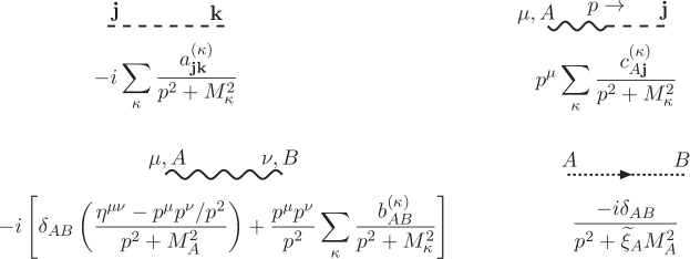
Figure 2.1: The scalar, massive vector $Z_{A}^{\mu}$, and corresponding ghost propagators, in the general case of arbitrary mixing between Goldstone scalars and other scalar and vector bosons. The squared mass poles $M^{2}_{\kappa}$ arise as the roots of a polynomial of order $N$ in $-p^{2}$, where $N$ is the total number of real scalar bosons and massive vector bosons, with $\kappa=1,\ldots,N$.

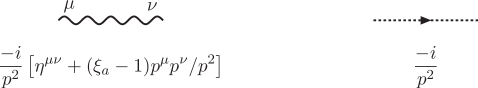
Figure 2.2: Feynman rules for the propagators of the massless vectors $A_{\mu}^{a}$ (wavy lines), and the corresponding massless ghosts $\overline{\eta}^{a},\eta^{a}$ (dotted lines with arrows), each carrying 4-momentum $p^{\mu}$.

The massless vectors and their corresponding ghosts are unmixed, and their propagator Feynman rules are shown in Figure 2.2. The two-component fermion propagators follow from eq. (1.5) in the usual way Dreiner:2008tw ; Martin:2012us , and are shown in Figure 2.3.

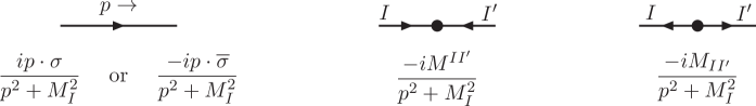
Figure 2.3: Feynman rules for the propagators of the two-component fermions (using the conventions of Dreiner:2008tw ; Martin:2012us ), each carrying 4-momentum $p^{\mu}$. The arrows follow the helicity, and the large dots represent fermion mass insertions.

The interaction part of the Lagrangian can now be written in the form:

$${\cal L}_{\rm int} = -\frac{1}{6}\lambda^{\bf jkl}R_{\bf j}R_{\bf k}R_{\bf l}-\frac{1}{24}\lambda^{\bf jklm}R_{\bf j}R_{\bf k}R_{\bf l}R_{\bf m}-\frac{1}{2}(Y^{{\bf j}IJ}R_{\bf j}\psi_{I}\psi_{J}+{\rm c.c.})$$ (2.28)

$$+g_{I}^{{\bf a}J}A^{\bf a}_{\mu}\psi^{\dagger I}\overline{\sigma}^{\mu}\psi_{J}-g^{\bf a}_{\bf jk}A_{\mu}^{\bf a}R_{\bf j}\partial^{\mu}R_{\bf k}-\frac{1}{2}g^{\bf a}_{\bf jn}g^{\bf b}_{\bf kn}A_{\mu}^{\bf a}A^{\mu\bf b}R_{\bf j}R_{\bf k}$$

$$-g^{\bf a}_{A\bf j}M_{A}R_{\bf j}Z_{\mu}^{A}A^{\mu\bf a}-g^{\bf a}_{A\bf j}\widetilde{\xi}_{A}M_{A}R_{\bf j}\overline{\eta}^{A}\eta^{\bf a}$$

$$-g^{\bf abc}A^{\mu\bf a}A^{\nu\bf b}\partial_{\mu}A^{\bf c}_{\nu}-\frac{1}{4}g^{\bf abe}g^{\bf cde}A^{\mu\bf a}A^{\nu\bf b}A_{\mu}^{\bf c}A_{\nu}^{\bf d}+g^{\bf abc}A_{\mu}^{\bf a}\eta^{\bf b}\partial^{\mu}\overline{\eta}^{\bf c},$$

where the $\phi$-dependent (scalar)³ and (scalar)⁴ couplings are defined from the tree-level scalar potential by

$$\lambda^{\bf jkl} = \frac{\partial^{3}V}{\partial R_{\bf j}\partial R_{\bf k}\partial R_{\bf l}}\Bigl{|}_{R_{\bf n}=0},$$ (2.29)

$$\lambda^{\bf jklm} = \frac{\partial^{4}V}{\partial R_{\bf j}\partial R_{\bf k}\partial R_{\bf l}\partial R_{\bf m}}.$$ (2.30)

The interaction vertex Feynman rules can be obtained in the usual way, and are shown in Figure 2.4. Here we have defined a vector-vector-scalar coupling $G^{\bf ab}_{\bf j}$ in terms of the scalar-scalar-vector coupling, according to:

$$G^{ab}_{\bf j} = 0,$$ (2.31)

$$G^{Aa}_{\bf j} = G^{aA}_{\bf j}\>=\>g^{a}_{A\bf j}M_{A},$$ (2.32)

$$G^{AB}_{\bf j} = g^{B}_{A\bf j}M_{A}+g^{A}_{B\bf j}M_{B}.$$ (2.33)

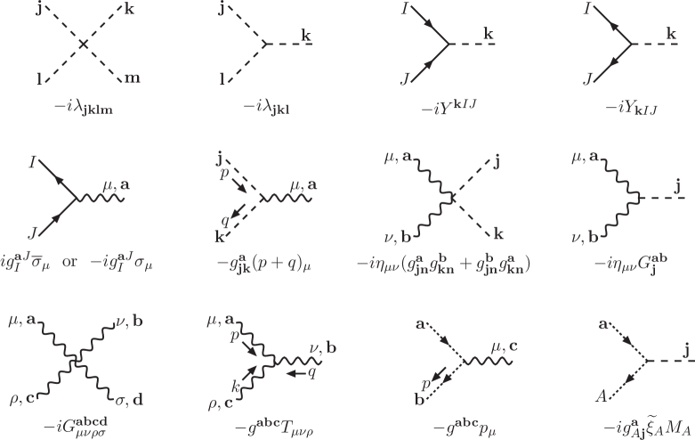
Figure 2.4: Feynman rules for interactions. Dashed lines represent scalars, solid lines with arrows represent fermions, wavy lines represent vectors, and dotted lines with arrows represent ghosts. Bold-faced letters from the beginning of the alphabet ($\bf a$, $\bf b$, $\bf c$, $\ldots$) run over all real vectors in the theory and their corresponding ghosts and anti-ghosts. Bold-faced letters from the middle of the alphabet ($\bf j$, $\bf k$, $\bf l$, $\ldots$) run over all of the real scalars in the theory. Capital letters from the middle of the alphabet $(I,J,\ldots)$ represent two-component fermions. The vector-vector-scalar coupling $G^{\bf ab}_{\bf j}$ is given by eqs. (2.31)-(2.33). The (vector)⁴ coupling is defined by $G^{\bf abcd}_{\mu\nu\rho\sigma}=g^{\bf abe}g^{\bf cde}[\eta_{\mu\rho}\eta_{\nu\sigma}-\eta_{\mu\sigma}\eta_{\nu\rho}]+g^{\bf ace}g^{\bf bde}[\eta_{\mu\nu}\eta_{\rho\sigma}-\eta_{\mu\sigma}\eta_{\nu\rho}]+g^{\bf ade}g^{\bf bce}[\eta_{\mu\nu}\eta_{\rho\sigma}-\eta_{\mu\rho}\eta_{\nu\sigma}].$ The (vector)³ coupling tensor is defined by $T_{\mu\nu\rho}=\eta_{\mu\nu}(p-q)_{\rho}+\eta_{\nu\rho}(q-k)_{\mu}+\eta_{\mu\rho}(k-p)_{\nu}$. In the last, ghost-antighost-scalar, interaction, the index $A$ corresponds to a vector with non-zero physical mass.

III Effective potential at two-loop order

III.1 General form

In this section we present the results for the effective potential, with the general gauge fixing described above.

The 1-loop effective potential contribution is:

$$V^{(1)} = \sum_{\kappa}f(\kappa)-2\sum_{I}f(I)+\sum_{A}[3f_{V}(A)-2f(A_{\eta})].$$ (3.1)

where $f(x)$ and $f_{V}(x)$ are renormalization scheme-dependent loop integral functions, which will be given below in the bare and $\overline{\rm{MS}}$ renormalization schemes. Here and below, we use a notation in which an index is used as a synonym for the squared mass whenever it appears as the argument of a loop integral function. For example, in eq. (3.1), $\kappa$ stands for $M_{\kappa}^{2}$, and $I$ stands for $M_{I}^{2}$, and $A$ for $M_{A}^{2}$, and we also use

$$A_{\eta} = \widetilde{\xi}_{A}M_{A}^{2},$$ (3.2)

$$a_{\eta} = 0$$ (3.3)

for the ghost squared masses.

For the 2-loop effective potential, there are 23 non-vanishing Feynman diagrams, shown in Figure 3.1.

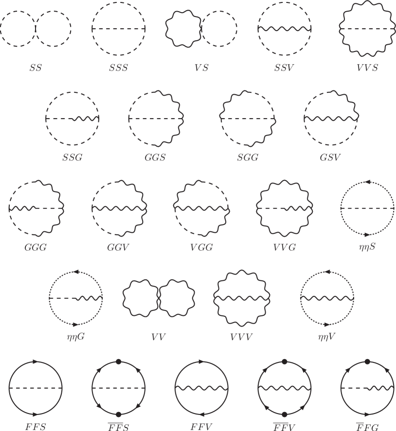
Figure 3.1: The non-vanishing 2-loop Feynman diagrams for the effective potential, for gauge-fixing choices that have propagator mixing between massive vectors and Goldstone scalars. Scalar bosons, fermions, vector bosons, and ghosts are represented by dashed, solid, wavy, and dotted lines, respectively. The arrows on fermion lines indicate the helicity, and large dots represent fermion mass insertions. For the $\overline{F}\overline{F}S$ and $\overline{F}FG$ diagrams, there are also diagrams with all fermion arrows reversed.

It follows that the two-loop contributions to the effective potential are given, in terms of the couplings and propagator parameters defined above, by:

$$V^{(2)}_{SS} = \frac{1}{8}\lambda^{\bf jklm}a_{\bf jk}^{(\kappa)}a_{\bf lm}^{(\sigma)}f_{SS}(\kappa,\sigma),$$ (3.4)

$$V^{(2)}_{SSS} = \frac{1}{12}\lambda^{\bf jkl}\lambda^{\bf mnp}a_{\bf jm}^{(\kappa)}a_{\bf kn}^{(\sigma)}a_{\bf lp}^{(\rho)}f_{SSS}(\kappa,\sigma,\rho),$$ (3.5)

$$V^{(2)}_{VS} = \frac{1}{2}g^{\bf a}_{\bf jk}g^{\bf a}_{\bf jl}a^{(\kappa)}_{\bf kl}f_{VS}({\bf a},\kappa)+\frac{1}{2}g^{A}_{\bf jk}g^{B}_{\bf jl}a^{(\kappa)}_{\bf kl}b^{(\sigma)}_{AB}f_{\overline{V}S}(\sigma,\kappa),$$ (3.6)

$$V^{(2)}_{SSV} = \frac{1}{4}g^{\bf a}_{\bf jk}g^{\bf a}_{\bf lm}a_{\bf jl}^{(\kappa)}a_{\bf km}^{(\sigma)}f_{SSV}(\kappa,\sigma,{\bf a})+\frac{1}{4}g^{A}_{\bf jk}g^{B}_{\bf lm}a_{\bf jl}^{(\kappa)}a_{\bf km}^{(\sigma)}b_{AB}^{(\rho)}f_{SS\overline{V}}(\kappa,\sigma,\rho),$$ (3.7)

$$V^{(2)}_{VVS} = \frac{1}{4}G^{\bf ab}_{\bf j}G^{\bf ab}_{\bf k}a_{\bf jk}^{(\kappa)}f_{VVS}({\bf a},{\bf b},\kappa)+\frac{1}{2}G^{{\bf a}A}_{\bf j}G^{{\bf a}B}_{\bf k}a_{\bf jk}^{(\kappa)}b_{AB}^{(\sigma)}f_{\overline{V}VS}(\sigma,{\bf a},\kappa)$$ (3.8)

$$+\frac{1}{4}G^{AB}_{\bf j}G^{CD}_{\bf k}a_{\bf jk}^{(\kappa)}b_{AC}^{(\sigma)}b_{BD}^{(\rho)}f_{\overline{V}\overline{V}S}(\sigma,\rho,\kappa),$$

$$V^{(2)}_{SSG} = \frac{1}{2}\lambda^{\bf jkl}g^{A}_{\bf mn}a_{\bf jm}^{(\kappa)}a_{\bf kn}^{(\sigma)}c_{A\bf l}^{(\rho)}f_{SSG}(\kappa,\sigma,\rho),$$ (3.9)

$$V^{(2)}_{GGS} = \frac{1}{2}\lambda^{\bf jkl}G^{AB}_{\bf m}a_{\bf jm}^{(\kappa)}c_{A\bf k}^{(\sigma)}c_{B\bf l}^{(\rho)}f_{GGS}(\sigma,\rho,\kappa),$$ (3.10)

$$V^{(2)}_{SGG} = \frac{1}{2}g^{A}_{\bf jk}g^{B}_{\bf lm}a_{\bf jl}^{(\kappa)}c_{A\bf l}^{(\sigma)}c_{B\bf k}^{(\rho)}f_{SGG}(\kappa,\sigma,\rho),$$ (3.11)

$$V^{(2)}_{GSV} = g^{\bf a}_{\bf jk}G^{A\bf a}_{\bf l}a_{\bf jl}^{(\kappa)}c_{A\bf k}^{(\sigma)}f_{GSV}(\sigma,\kappa,{\bf a})+g^{B}_{\bf jk}G^{AC}_{\bf l}a_{\bf jl}^{(\kappa)}c_{A\bf k}^{(\sigma)}b_{BC}^{(\rho)}f_{GS\overline{V}}(\sigma,\kappa,\rho),$$ (3.12)

$$V^{(2)}_{GGG} = \frac{1}{2}g^{C}_{\bf jk}G^{AB}_{\bf l}c_{A\bf j}^{(\kappa)}c_{B\bf k}^{(\sigma)}c_{C\bf l}^{(\rho)}f_{GGG}(\kappa,\sigma,\rho),$$ (3.13)

$$V^{(2)}_{GGV} = \frac{1}{2}g^{{\bf a}AB}g^{\bf a}_{\bf jk}c_{A\bf j}^{(\kappa)}c_{B\bf k}^{(\sigma)}f_{GGV}(\kappa,\sigma,{\bf a}),$$ (3.14)

$$V^{(2)}_{VGG} = \frac{1}{2}G^{A\bf a}_{\bf j}G^{B\bf a}_{\bf k}c_{A\bf k}^{(\kappa)}c_{B\bf j}^{(\sigma)}f_{VGG}({\bf a},\kappa,\sigma)+\frac{1}{2}G^{AC}_{\bf j}G^{BD}_{\bf k}c_{A\bf k}^{(\kappa)}c_{B\bf j}^{(\sigma)}b_{CD}^{(\rho)}f_{\overline{V}GG}(\rho,\kappa,\sigma),$$ (3.15)

$$V^{(2)}_{VVG} = \frac{1}{2}g^{{\bf ab}A}G^{\bf ab}_{\bf j}c_{A\bf j}^{(\kappa)}f_{VVG}({\bf a},{\bf b},\kappa)+g^{AB{\bf a}}G^{C\bf a}_{\bf j}c_{A\bf j}^{(\kappa)}b_{BC}^{(\sigma)}f_{\overline{V}VG}(\sigma,{\bf a},\kappa),$$ (3.16)

$$V^{(2)}_{\eta\eta S} = \frac{1}{2}g^{A}_{B\bf j}g^{B}_{A\bf k}\widetilde{\xi}_{A}\widetilde{\xi}_{B}M_{A}M_{B}a_{\bf jk}^{(\kappa)}f_{\eta\eta S}(A_{\eta},B_{\eta},\kappa),$$ (3.17)

$$V^{(2)}_{\eta\eta G} = g^{{\bf a}AB}g^{\bf a}_{A\bf j}\widetilde{\xi}_{A}M_{A}c_{B\bf j}^{(\kappa)}f_{\eta\eta G}({\bf a}_{\eta},A_{\eta},\kappa),$$ (3.18)

$$V^{(2)}_{VV} = \frac{1}{4}\bigl{(}g^{\bf abc}\bigr{)}^{2}f_{VV}({\bf a},{\bf b})+\frac{1}{2}g^{{\bf ab}A}g^{{\bf ab}B}b_{AB}^{(\kappa)}f_{\overline{V}V}(\kappa,{\bf a})$$ (3.19)

$$+\frac{1}{4}g^{{\bf a}AB}g^{{\bf a}CD}b_{AC}^{(\kappa)}b_{BD}^{(\sigma)}f_{\overline{V}\overline{V}}(\kappa,\sigma),$$

$$V^{(2)}_{VVV} = \frac{1}{12}\bigl{(}g^{\bf abc}\bigr{)}^{2}f_{VVV}({\bf a},{\bf b},{\bf c})+\frac{1}{4}g^{{\bf ab}A}g^{{\bf ab}B}b_{AB}^{(\kappa)}f_{\overline{V}VV}(\kappa,{\bf a},{\bf b})$$ (3.20)

$$+\frac{1}{4}g^{{\bf a}AB}g^{{\bf a}CD}b_{AC}^{(\kappa)}b_{BD}^{(\sigma)}f_{\overline{V}\overline{V}V}(\kappa,\sigma,{\bf a}),$$

$$V^{(2)}_{\eta\eta V} = \frac{1}{4}\bigl{(}g^{\bf abc}\bigr{)}^{2}f_{\eta\eta V}({\bf a}_{\eta},{\bf b}_{\eta},{\bf c})+\frac{1}{4}g^{{\bf ab}A}g^{{\bf ab}B}b_{AB}^{(\kappa)}f_{\eta\eta\overline{V}}({\bf a}_{\eta},{\bf b}_{\eta},\kappa),$$ (3.21)

$$V^{(2)}_{FFS} = \frac{1}{2}Y^{{\bf j}IJ}Y_{{\bf k}IJ}a_{\bf jk}^{(\kappa)}f_{FFS}(I,J,\kappa),$$ (3.22)

$$V^{(2)}_{\overline{F}\overline{F}S} = \frac{1}{4}(Y^{{\bf j}IJ}Y^{{\bf k}I^{\prime}J^{\prime}}M_{II^{\prime}}M_{JJ^{\prime}}+{\rm c.c.})a_{\bf jk}^{(\kappa)}f_{\overline{F}\overline{F}S}(I,J,\kappa),$$ (3.23)

$$V^{(2)}_{FFV} = \frac{1}{2}g^{{\bf a}J}_{I}g^{{\bf a}I}_{J}f_{FFV}(I,J,{\bf a})+\frac{1}{2}g^{AJ}_{I}g^{BI}_{J}b_{AB}^{(\kappa)}f_{FF\overline{V}}(I,J,\kappa),$$ (3.24)

$$V^{(2)}_{\overline{F}\overline{F}V} = \frac{1}{2}g^{{\bf a}J}_{I}g^{{\bf a}J^{\prime}}_{I^{\prime}}M^{II^{\prime}}M_{JJ^{\prime}}f_{\overline{F}\overline{F}V}(I,J,{\bf a})+\frac{1}{2}g^{AJ}_{I}g^{BJ^{\prime}}_{I^{\prime}}M^{II^{\prime}}M_{JJ^{\prime}}b_{AB}^{(\kappa)}f_{\overline{F}\overline{F}\overline{V}}(I,J,\kappa),$$ (3.25)

$$V^{(2)}_{\overline{F}FG} = i\left(g^{AJ}_{I}Y_{jI^{\prime}J}M^{II^{\prime}}-{\rm c.c.}\right)c_{A\bf j}^{(\kappa)}f_{\overline{F}FG}(I,J,\kappa).$$ (3.26)

In these equations, all indices (including $\kappa,\sigma,\rho$) are summed over in each term.

It remains to find the following 37 two-loop integral functions:

$$f_{SS}(x,y),\>\>\>\>f_{SSS}(x,y,z),\>\>\>\>f_{VS}(x,y),\>\>\>\>f_{\overline{V}S}(x,y),\>\>\>\>f_{SSV}(x,y,z),\>\>\>\>$$

$$f_{SS\overline{V}}(x,y,z),\>\>\>\>f_{VVS}(x,y,z),\>\>\>\>f_{\overline{V}VS}(x,y,z),\>\>\>\>f_{\overline{V}\overline{V}S}(x,y,z),\>\>\>\>f_{SSG}(x,y,z),\>\>\>\>$$

$$f_{GGS}(x,y,z),\>\>\>\>f_{SGG}(x,y,z),\>\>\>\>f_{GSV}(x,y,z),\>\>\>\>f_{GS\overline{V}}(x,y,z),\>\>\>\>f_{GGG}(x,y,z),\>\>\>\>$$

$$f_{GGV}(x,y,z),\>\>\>\>f_{VGG}(x,y,z),\>\>\>\>f_{\overline{V}GG}(x,y,z),\>\>\>\>f_{VVG}(x,y,z),\>\>\>\>$$

$$f_{\overline{V}VG}(x,y,z),\>\>\>\>f_{\eta\eta S}(x,y,z),\>\>\>\>f_{\eta\eta G}(x,y,z),\>\>\>\>f_{VV}(x,y),\>\>\>\>$$

$$f_{\overline{V}V}(x,y),\>\>\>\>f_{\overline{V}\overline{V}}(x,y),\>\>\>\>f_{VVV}(x,y,z),\>\>\>\>f_{\overline{V}VV}(x,y,z),\>\>\>\>f_{\overline{V}\overline{V}V}(x,y,z),\>\>\>\>$$

$$f_{\eta\eta V}(x,y,z),\>\>\>\>f_{\eta\eta\overline{V}}(x,y,z),\>\>\>\>f_{FFS}(x,y,z),\>\>\>\>f_{\overline{F}\overline{F}S}(x,y,z),\>\>\>\>$$

$$f_{FFV}(x,y,z),\>\>\>\>f_{FF\overline{V}}(x,y,z),\>\>\>\>f_{\overline{F}\overline{F}V}(x,y,z),\>\>\>\>f_{\overline{F}\overline{F}\overline{V}}(x,y,z),\>\>\>\>f_{\overline{F}FG}(x,y,z).$$ (3.27)

In the next subsection III.2, we present the results for the loop integration functions in the case that all parameters of the theory are taken to be bare parameters using dimensional regularization Bollini:1972ui ; Ashmore:1972uj ; Cicuta:1972jf ; tHooft:1972fi ; tHooft:1973mm . In subsection III.3, we present the result in the more practically relevant case that all parameters are renormalized in the $\overline{\rm{MS}}$ Bardeen:1978yd ; Braaten:1981dv scheme. In both cases, we write the results in terms of 1-loop and 2-loop basis vacuum integrals following the conventions of refs. Martin:2001vx ; Martin:2017lqn ; these are reviewed for convenience in Appendix A below.

III.2 Results for two-loop effective potential functions in terms of bare parameters

In this section, we report the results for the 2-loop effective potential in terms of bare parameters. This means that all of the masses and couplings appearing in eqs. (3.1) and (3.4)-(3.26) are the bare ones, and the corresponding loop integral functions will be distinguished by using $\bf f$ in place of $f$ in the names of the functions. Then then 1-loop integrals appearing in eq. (3.1) are:

$${\bf f}(x) = x{\bf A}(x)/d,$$ (3.28)

$${\bf f}_{V}(x) = (d-1)x{\bf A}(x)/3d.$$ (3.29)

(The notations for the basis integrals ${\bf A}(x)$ and ${\bf I}(x,y,z)$ are reviewed in Appendix A.) For the two-loop integrals appearing in eqs. (3.4)-(3.26), we obtain:

$${\bf f}_{SSS}(x,y,z) = -{\bf I}(x,y,z),$$ (3.30)

$${\bf f}_{SS}(x,y) = {\bf A}(x){\bf A}(y),$$ (3.31)

$${\bf f}_{VS}(x,y) = (d-1){\bf A}(x){\bf A}(y),$$ (3.32)

$${\bf f}_{\overline{V}S}(x,y) = {\bf A}(x){\bf A}(y),$$ (3.33)

$${\bf f}_{SSV}(x,y,z) = \frac{1}{z}\Bigl{[}-\lambda(x,y,z){\bf I}(x,y,z)+(x-y)^{2}{\bf I}(0,x,y)+z{\bf A}(x){\bf A}(y)$$ (3.34)

$$+(y-x-z){\bf A}(x){\bf A}(z)+(x-y-z){\bf A}(y){\bf A}(z)\Bigr{]},$$

$${\bf f}_{SS\overline{V}}(x,y,z) = \frac{1}{z}\Bigl{\{}(x-y)^{2}[{\bf I}(x,y,z)-{\bf I}(0,x,y)]+(x-y-z){\bf A}(x){\bf A}(z)$$ (3.35)

$$+(y-x-z){\bf A}(y){\bf A}(z)\Bigr{\}},$$

$${\bf f}_{\overline{V}\overline{V}S}(x,y,z) = \frac{1}{4xy}\Bigl{[}-(x+y-z)^{2}{\bf I}(x,y,z)+(x-z)^{2}{\bf I}(0,x,z)+(y-z)^{2}{\bf I}(0,y,z)$$ (3.36)

$$-z^{2}{\bf I}(0,0,z)+(z-x-y){\bf A}(x){\bf A}(y)+y{\bf A}(x){\bf A}(z)+x{\bf A}(y){\bf A}(z)\Bigr{]},$$

$${\bf f}_{\overline{V}VS}(x,y,z) = -{\bf f}_{\overline{V}\overline{V}S}(x,y,z)-{\bf I}(x,y,z),$$ (3.37)

$${\bf f}_{VVS}(x,y,z) = {\bf f}_{\overline{V}\overline{V}S}(x,y,z)+(2-d){\bf I}(x,y,z),$$ (3.38)

$${\bf f}_{SSG}(x,y,z) = (x-y){\bf I}(x,y,z)+[{\bf A}(x)-{\bf A}(y)]{\bf A}(z),$$ (3.39)

$${\bf f}_{GGS}(x,y,z) = \frac{1}{2}\Bigl{[}(x+y-z){\bf I}(x,y,z)+{\bf A}(x){\bf A}(y)-{\bf A}(x){\bf A}(z)-{\bf A}(y){\bf A}(z)\Bigr{]},$$ (3.40)

$${\bf f}_{SGG}(x,y,z) = -(x-y)(x-z){\bf I}(x,y,z)+(y-x){\bf A}(x){\bf A}(y)+(z-x){\bf A}(x){\bf A}(z)$$ (3.41)

$$+x{\bf A}(y){\bf A}(z),$$

$${\bf f}_{GSV}(x,y,z) = -\frac{1}{2}{\bf f}_{SSV}(x,y,z),$$ (3.42)

$${\bf f}_{GS\overline{V}}(x,y,z) = \frac{1}{2z}\Bigl{[}(y-x)(x-y+z){\bf I}(x,y,z)+(x-y)^{2}{\bf I}(0,x,y)$$ (3.43)

$$+(x-y+2z){\bf A}(y){\bf A}(z)+(y-x){\bf A}(x){\bf A}(z)\Bigr{]},$$

$${\bf f}_{GGG}(x,y,z) = \frac{1}{2}\bigl{\{}(x-y)[(z-x-y){\bf I}(x,y,z)-{\bf A}(x){\bf A}(y)]$$ (3.44)

$$+(x+y)[{\bf A}(y)-{\bf A}(x)]{\bf A}(z)\bigr{\}},$$

$${\bf f}_{GGV}(x,y,z) = \frac{1}{2}\bigl{[}\lambda(x,y,z){\bf I}(x,y,z)+(x+y-z){\bf A}(x){\bf A}(y)$$ (3.45)

$$+(x+z-y){\bf A}(x){\bf A}(z)+(y+z-x){\bf A}(y){\bf A}(z)\bigr{]},$$

$${\bf f}_{VGG}(x,y,z) = \frac{1}{4x}\bigl{[}\lambda(x,y,z){\bf I}(x,y,z)-(y-z)^{2}{\bf I}(0,y,z)+(x+y-z){\bf A}(x){\bf A}(y)$$ (3.46)

$$+(x-y+z){\bf A}(x){\bf A}(z)-x{\bf A}(y){\bf A}(z)\bigr{]},$$

$${\bf f}_{\overline{V}GG}(x,y,z) = \frac{1}{4x}\bigl{[}(x+y-z)(x+z-y){\bf I}(x,y,z)+(y-z)^{2}{\bf I}(0,y,z)-x{\bf A}(y){\bf A}(z)$$ (3.47)

$$+(x+y-z){\bf A}(x){\bf A}(z)+(x+z-y){\bf A}(x){\bf A}(y)\bigr{]},$$

$${\bf f}_{VVG}(x,y,z) = \frac{1}{4xy}\Bigl{\{}(x-y)[\lambda(x,y,z)+4(d-1)xy]{\bf I}(x,y,z)-x(x-z)^{2}{\bf I}(0,x,z)$$ (3.48)

$$+y(y-z)^{2}{\bf I}(0,y,z)+(x-y)(x+y-z){\bf A}(x){\bf A}(y)$$

$$+y[(4d-6)x+y-z]{\bf A}(x){\bf A}(z)-x[(4d-6)y+x-z]{\bf A}(y){\bf A}(z)\Bigr{\}},$$

$${\bf f}_{\overline{V}VG}(x,y,z) = -\frac{1}{4}{\bf f}_{SSV}(z,y,x),$$ (3.49)

$${\bf f}_{\eta\eta S}(x,y,z) = {\bf I}(x,y,z),$$ (3.50)

$${\bf f}_{\eta\eta G}(x,y,z) = -{\bf f}_{GGS}(x,z,y),$$ (3.51)

$${\bf f}_{VV}(x,y) = \frac{(d-1)^{3}}{d}{\bf A}(x){\bf A}(y),$$ (3.52)

$${\bf f}_{\overline{V}V}(x,y) = \frac{(d-1)^{2}}{d}{\bf A}(x){\bf A}(y),$$ (3.53)

$${\bf f}_{\overline{V}\overline{V}}(x,y) = \frac{(d-1)}{d}{\bf A}(x){\bf A}(y),$$ (3.54)

$${\bf f}_{VVV}(x,y,z) = \frac{1}{4xyz}\Bigl{\{}-\lambda(x,y,z)[\lambda(x,y,z)+4(d-1)(xy+xz+yz)]{\bf I}(x,y,z)$$ (3.55)

$$+(x-y)^{2}[x^{2}+y^{2}+(4d-6)xy]{\bf I}(0,x,y)-z^{4}{\bf I}(0,0,z)$$

$$+(x-z)^{2}[x^{2}+z^{2}+(4d-6)xz]{\bf I}(0,x,z)-y^{4}{\bf I}(0,0,y)$$

$$+(y-z)^{2}[y^{2}+z^{2}+(4d-6)yz]{\bf I}(0,y,z)-x^{4}{\bf I}(0,0,x)$$

$$+[(7-4d)(x^{2}+y^{2}-xz-yz)+(2-4d+4/d)xy+z^{2}]z{\bf A}(x){\bf A}(y)$$

$$+[(7-4d)(x^{2}+z^{2}-xy-yz)+(2-4d+4/d)xz+y^{2}]y{\bf A}(x){\bf A}(z)$$

$$+[(7-4d)(y^{2}+z^{2}-xy-xz)+(2-4d+4/d)yz+x^{2}]x{\bf A}(y){\bf A}(z)\Bigr{\}},$$

$${\bf f}_{\overline{V}VV}(x,y,z) = \frac{1}{4xyz}\Bigl{\{}(y-z)^{2}[\lambda(x,y,z)+4(d-1)yz]{\bf I}(x,y,z)$$ (3.56)

$$-(y-z)^{2}[y^{2}+z^{2}+(4d-6)yz]{\bf I}(0,y,z)-(x-z)^{2}z^{2}{\bf I}(0,x,z)$$

$$-(x-y)^{2}y^{2}{\bf I}(0,x,y)+y^{4}{\bf I}(0,0,y)+z^{4}{\bf I}(0,0,z)-x(y-z)^{2}{\bf A}(y){\bf A}(z)$$

$$+[(7-4d)y(z-y)+(x-z)z+(6-4d-4/d)xy]z{\bf A}(x){\bf A}(y)$$

$$+[(7-4d)z(y-z)+(x-y)y+(6-4d-4/d)xz]y{\bf A}(x){\bf A}(z)\Bigr{\}},$$

$${\bf f}_{\overline{V}\overline{V}V}(x,y,z) = \frac{1}{4xy}\Bigl{\{}-z\lambda(x,y,z){\bf I}(x,y,z)+(x-z)^{2}z{\bf I}(0,x,z)+(y-z)^{2}z{\bf I}(0,y,z)$$ (3.57)

$$-z^{3}{\bf I}(0,0,z)+[z^{2}-xz-yz+4xy(1/d-1)]{\bf A}(x){\bf A}(y)$$

$$+z[x{\bf A}(y)+y{\bf A}(x)]{\bf A}(z)\Bigr{\}},$$

$${\bf f}_{\eta\eta V}(x,y,z) = \frac{1}{2z}\bigl{[}\lambda(x,y,z){\bf I}(x,y,z)-(x-y)^{2}{\bf I}(0,x,y)$$ (3.58)

$$-z{\bf A}(x){\bf A}(y)+(x-y+z){\bf A}(x){\bf A}(z)+(y-x+z){\bf A}(y){\bf A}(z)\bigr{]},$$

$${\bf f}_{\eta\eta\overline{V}}(x,y,z) = \frac{1}{2z}\bigl{[}(y-x-z)(x-y-z){\bf I}(x,y,z)+(x-y)^{2}{\bf I}(0,x,y)-z{\bf A}(x){\bf A}(y)$$ (3.59)

$$+(y-x+z){\bf A}(x){\bf A}(z)+(x-y+z){\bf A}(y){\bf A}(z)\bigr{]},$$

$${\bf f}_{FFS}(x,y,z) = (x+y-z){\bf I}(x,y,z)+{\bf A}(x){\bf A}(y)-{\bf A}(x){\bf A}(z)-{\bf A}(y){\bf A}(z),$$ (3.60)

$${\bf f}_{\overline{F}\overline{F}S}(x,y,z) = 2{\bf I}(x,y,z),$$ (3.61)

$${\bf f}_{FFV}(x,y,z) = \frac{1}{z}\Bigl{\{}[\lambda(x,y,z)+(d-1)z(x+y-z)]{\bf I}(x,y,z)-(x-y)^{2}{\bf I}(0,x,y)$$ (3.62)

$$+[x-y+(2-d)z]{\bf A}(x){\bf A}(z)+[y-x+(2-d)z]{\bf A}(y){\bf A}(z)$$

$$+(d-2)z{\bf A}(x){\bf A}(y)\Bigr{\}},$$

$${\bf f}_{FF\overline{V}}(x,y,z) = \frac{1}{z}\bigl{\{}(xz+yz-x^{2}+2xy-y^{2}){\bf I}(x,y,z)+(x-y)^{2}{\bf I}(0,x,y)$$ (3.63)

$$+(x-y)[{\bf A}(y)-{\bf A}(x)]{\bf A}(z)\bigr{\}},$$

$${\bf f}_{\overline{F}\overline{F}V}(x,y,z) = 2(d-1){\bf I}(x,y,z),$$ (3.64)

$${\bf f}_{\overline{F}\overline{F}\overline{V}}(x,y,z) = 2{\bf I}(x,y,z),$$ (3.65)

$${\bf f}_{\overline{F}FG}(x,y,z) = (y+z-x){\bf I}(x,y,z)-{\bf A}(x){\bf A}(y)-{\bf A}(x){\bf A}(z)+{\bf A}(y){\bf A}(z).$$ (3.66)

III.3 Results in terms of $\overline{\rm{MS}}$ parameters

In this subsection, we provide the results for the effective potential loop integral functions, this time as they appear in in the $\overline{\rm{MS}}$ scheme with renormalization scale $Q$, and $\overline{\ln}(x)\equiv\ln(x/Q^{2})$, and renormalized basis integrals $A(x)$ and $I(x,y,z)$ given in Appendix A.

The one-loop functions for the $\overline{\rm{MS}}$ scheme can be obtained from the ones for the bare scheme by including counterterms for the ultraviolet 1-loop sub-divergences, and then taking the limit as $\epsilon\rightarrow 0$. One has

$$f(x) = \lim_{\epsilon\rightarrow 0}\Bigl{[}{\bf f}(x)+\frac{x^{2}}{4\epsilon}\Bigr{]},$$ (3.67)

$$f_{V}(x) = \lim_{\epsilon\rightarrow 0}\Bigl{[}{\bf f}_{V}(x)+\frac{x^{2}}{4\epsilon}\Bigr{]},$$ (3.68)

with the results:

$$f(x) = \frac{x^{2}}{4}\bigl{[}\overline{\ln}(x)-3/2],$$ (3.69)

$$f_{V}(x) = \frac{x^{2}}{4}\bigl{[}\overline{\ln}(x)-5/6],$$ (3.70)

which should be used in eq. (3.1) for the $\overline{\rm{MS}}$ scheme.

Similarly, the two-loop functions appearing in eqs. (3.4)-(3.26) in the $\overline{\rm{MS}}$ scheme can be obtained by taking the limit $\epsilon\rightarrow 0$ after including counterterms for the 1-loop and 2-loop sub-divergences. The 2-loop counterterms are determined by modified minimal subtraction and the requirement that the resulting functions are finite as $\epsilon\rightarrow 0$. The inclusions of counterterms are as follows:

$$f_{SSS}(x,y,z) = \lim_{\epsilon\rightarrow 0}\Bigl{\{}{\bf f}_{SSS}(x,y,z)+\frac{1}{2\epsilon^{2}}(x+y+z)-\frac{1}{2\epsilon}(x+y+z)$$ (3.71)

$$+\frac{1}{\epsilon}\left[{\bf A}(x)+{\bf A}(y)+{\bf A}(z)\right]\Bigr{\}},$$

$$f_{SS}(x,y) = \lim_{\epsilon\rightarrow 0}\Bigl{\{}{\bf f}_{SS}+\frac{1}{\epsilon^{2}}xy+\frac{1}{\epsilon}\left[y{\bf A}(x)+x{\bf A}(y)\right]\Bigr{\}},$$ (3.72)

$$f_{VS}(x,y) = \lim_{\epsilon\rightarrow 0}\Bigl{\{}{\bf f}_{VS}+\frac{3}{\epsilon^{2}}xy+\frac{1}{\epsilon}\left[(d-1)y{\bf A}(x)+3x{\bf A}(y)\right]\Bigr{\}},$$ (3.73)

$$f_{\overline{V}S}(x,y) = \lim_{\epsilon\rightarrow 0}\Bigl{\{}{\bf f}_{\overline{V}S}+\frac{1}{\epsilon^{2}}xy+\frac{1}{\epsilon}\left[y{\bf A}(x)+x{\bf A}(y)\right]\Bigr{\}},$$ (3.74)

$$f_{SSV}(x,y,z) = \lim_{\epsilon\rightarrow 0}\Bigl{\{}{\bf f}_{SSV}(x,y,z)+\frac{1}{2\epsilon^{2}}\left(-3x^{2}-3y^{2}-3xz-3yz+z^{2}\right)$$ (3.75)

$$+\frac{1}{6\epsilon}\left(3x^{2}+3y^{2}-7z^{2}+18xy+15xz+15yz\right)$$

$$+\frac{1}{\epsilon}\left[-3x{\bf A}(x)-3y{\bf A}(y)+(1-d)(x+y-z/3){\bf A}(z)\right]\Bigr{\}},$$

$$f_{SS\overline{V}}(x,y,z) = \lim_{\epsilon\rightarrow 0}\Bigl{\{}{\bf f}_{SS\overline{V}}(x,y,z)+\frac{1}{2\epsilon^{2}}[\lambda(x,y,z)-z^{2}]+\frac{1}{2\epsilon}(x-y)^{2}$$ (3.76)

$$+\frac{1}{\epsilon}\bigl{[}(x-y-z){\bf A}(x)+(y-x-z){\bf A}(y)-(x+y){\bf A}(z)\bigr{]}\Bigr{\}},$$

$$f_{VVS}(x,y,z) = \lim_{\epsilon\rightarrow 0}\Bigl{\{}{\bf f}_{VVS}(x,y,z)+\frac{1}{8\epsilon^{2}}(9x+9y+12z)+\frac{1}{8\epsilon}(2z-15x-15y)$$ (3.77)

$$+\frac{3}{4\epsilon}\left[(d-1){\bf A}(x)+(d-1){\bf A}(y)+4{\bf A}(z)\right]\Bigr{\}},$$

$$f_{\overline{V}VS}(x,y,z) = \lim_{\epsilon\rightarrow 0}\Bigl{\{}{\bf f}_{\overline{V}VS}(x,y,z)+\frac{3}{8\epsilon^{2}}(x+y)-\frac{1}{8\epsilon}(x+5y+6z)$$ (3.78)

$$+\frac{1}{4\epsilon}\left[3{\bf A}(x)+(d-1){\bf A}(y)\right]\Bigr{\}},$$

$$f_{\overline{V}\overline{V}S}(x,y,z) = \lim_{\epsilon\rightarrow 0}\Bigl{\{}{\bf f}_{\overline{V}\overline{V}S}(x,y,z)+\frac{1}{8\epsilon^{2}}(x+y+4z)+\frac{1}{8\epsilon}(-3x-3y+2z)$$ (3.79)

$$+\frac{1}{4\epsilon}\left[{\bf A}(x)+{\bf A}(y)+4{\bf A}(z)\right]\Bigr{\}},$$

$$f_{SSG}(x,y,z) = \lim_{\epsilon\rightarrow 0}\Bigl{\{}{\bf f}_{SSG}(x,y,z)+\frac{1}{2\epsilon^{2}}(x-y)(z-x-y)+\frac{1}{2\epsilon}(x-y)(x+y+z)$$ (3.80)

$$+\frac{1}{\epsilon}\left[(y-x+z){\bf A}(x)+(y-x-z){\bf A}(y)\right]\Bigr{\}},$$

$$f_{GGS}(x,y,z) = \lim_{\epsilon\rightarrow 0}\Bigl{\{}{\bf f}_{GGS}(x,y,z)+\frac{1}{4\epsilon^{2}}(z^{2}-x^{2}-y^{2}-2xz-2yz)+\frac{1}{4\epsilon}(x+y-z)(x+y+z)$$ (3.81)

$$+\frac{1}{2\epsilon}\left[-x{\bf A}(x)-y{\bf A}(y)+(z-2x-2y){\bf A}(z)\right]\Bigr{\}},$$

$$f_{SGG}(x,y,z) = \lim_{\epsilon\rightarrow 0}\Bigl{\{}{\bf f}_{SGG}(x,y,z)+\frac{1}{2\epsilon^{2}}(y+z-x)(xy+xz+yz-x^{2})$$ (3.82)

$$+\frac{1}{2\epsilon}(x-y)(z-x)(x+y+z)$$

$$+\frac{1}{\epsilon}\left[(\lambda(x,y,z)+3yz){\bf A}(x)+yz{\bf A}(y)+yz{\bf A}(z)\right]\Bigr{\}},$$

$$f_{GSV}(x,y,z) = \lim_{\epsilon\rightarrow 0}\Bigl{\{}{\bf f}_{GSV}(x,y,z)+\frac{1}{4\epsilon^{2}}(3x^{2}+3y^{2}+3xz+3yz-z^{2})$$ (3.83)

$$+\frac{1}{4\epsilon}(7z^{2}/3-x^{2}-6xy-y^{2}-5xz-5yz)$$

$$+\frac{1}{2\epsilon}\left[3x{\bf A}(x)+3y{\bf A}(y)+(d-1)(x+y-z/3){\bf A}(z)\right]\Bigr{\}},$$

$$f_{GS\overline{V}}(x,y,z) = \lim_{\epsilon\rightarrow 0}\Bigl{\{}{\bf f}_{GS\overline{V}}(x,y,z)+\frac{1}{4\epsilon^{2}}(2xy+xz+3yz-2y^{2})+\frac{1}{4\epsilon}(y-x)(2x+z)$$ (3.84)

$$+\frac{1}{\epsilon}\left[(x-y+z){\bf A}(y)+(x+y){\bf A}(z)/2\right]\Bigr{\}},$$

$$f_{GGG}(x,y,z) = \lim_{\epsilon\rightarrow 0}\Bigl{\{}{\bf f}_{GGG}(x,y,z)+\frac{1}{4\epsilon^{2}}(x-y)(x^{2}+y^{2}-z^{2}-2xz-2yz)$$ (3.85)

$$+\frac{1}{4\epsilon}(x-y)(z-x-y)(x+y+z)$$

$$+\frac{1}{2\epsilon}\left[x(x-y-2z){\bf A}(x)+y(x-y+2z){\bf A}(y)+(y-x)z{\bf A}(z)\right]\Bigr{\}},$$

$$f_{GGV}(x,y,z) = \lim_{\epsilon\rightarrow 0}\Bigl{\{}{\bf f}_{GGV}(x,y,z)$$ (3.86)

$$+\frac{1}{4\epsilon^{2}}(-x^{3}-y^{3}-z^{3}+3x^{2}y+3xy^{2}+3x^{2}z+3xz^{2}+3y^{2}z+3yz^{2})$$

$$+\frac{1}{4\epsilon}(x^{3}+y^{3}+7z^{3}/3-x^{2}y-xy^{2}-x^{2}z-y^{2}z-5xz^{2}-5yz^{2}-6xyz)$$

$$+\frac{1}{2\epsilon}\bigl{[}x(3y+3z-x){\bf A}(x)+y(3x+3z-y){\bf A}(y)$$

$$+(d-1)z(x+y-z/3){\bf A}(z)\bigr{]}\Bigr{\}},$$

$$f_{VGG}(x,y,z) = \lim_{\epsilon\rightarrow 0}\Bigl{\{}{\bf f}_{VGG}(x,y,z)+\frac{1}{8\epsilon^{2}}(3y^{2}+3z^{2}-x^{2}+3xy+3xz)$$ (3.87)

$$+\frac{1}{8\epsilon}(7x^{2}/3-y^{2}-z^{2}-5xy-5xz-6yz)$$

$$+\frac{1}{4\epsilon}\left[(d-1)(y+z-x/3){\bf A}(x)+3y{\bf A}(y)+3z{\bf A}(z)\right]\Bigr{\}},$$

$$f_{\overline{V}GG}(x,y,z) = \lim_{\epsilon\rightarrow 0}\Bigl{\{}{\bf f}_{\overline{V}GG}(x,y,z)+\frac{1}{8\epsilon^{2}}(xy+xz-x^{2}-y^{2}-z^{2})$$ (3.88)

$$+\frac{1}{8\epsilon}(x^{2}-y^{2}-z^{2}+xy+xz+2yz)$$

$$+\frac{1}{4\epsilon}\left[(y+z-x){\bf A}(x)-y{\bf A}(y)-z{\bf A}(z)\right]\Bigr{\}},$$

$$f_{VVG}(x,y,z) = \lim_{\epsilon\rightarrow 0}\Bigl{\{}{\bf f}_{VVG}(x,y,z)+\frac{1}{\epsilon^{2}}(x-y)(9z/8-x-y)$$ (3.89)

$$+\frac{1}{24\epsilon}(x-y)(38x+38y+9z)$$

$$+\frac{1}{12\epsilon}(d-1)\left[(9y+9z-8x){\bf A}(x)-(9x+9z-8y){\bf A}(y)\right]\Bigr{\}},$$

$$f_{\overline{V}VG}(x,y,z) = \lim_{\epsilon\rightarrow 0}\Bigl{\{}{\bf f}_{\overline{V}VG}(x,y,z)+\frac{1}{8\epsilon^{2}}(3y^{2}+3z^{2}-x^{2}+3xy+3xz)$$ (3.90)

$$+\frac{1}{8\epsilon}(x^{2}-5y^{2}-z^{2}-xy-xz-6yz)$$

$$+\frac{1}{4\epsilon}\left[(3y+3z-x){\bf A}(x)+(d-1)y{\bf A}(y)+3z{\bf A}(z)\right]\Bigr{\}},$$

$$f_{\eta\eta S}(x,y,z) = \lim_{\epsilon\rightarrow 0}\Bigl{\{}{\bf f}_{\eta\eta S}(x,y,z)-\frac{1}{2\epsilon^{2}}(x+y+z)+\frac{1}{2\epsilon}(x+y+z)$$ (3.91)

$$-\frac{1}{\epsilon}\left[{\bf A}(x)+{\bf A}(y)+{\bf A}(z)\right]\Bigr{\}},$$

$$f_{\eta\eta G}(x,y,z) = \lim_{\epsilon\rightarrow 0}\Bigl{\{}{\bf f}_{\eta\eta G}(x,y,z)+\frac{1}{4\epsilon^{2}}(x^{2}-y^{2}+z^{2}+2xy+2yz)+\frac{1}{4\epsilon}(y-x-z)(x+y+z)$$ (3.92)

$$+\frac{1}{2\epsilon}\left[x{\bf A}(x)+(2x-y+2z){\bf A}(y)+z{\bf A}(z)\right]\Bigr{\}},$$

$$f_{VV}(x,y) = \lim_{\epsilon\rightarrow 0}\Bigl{\{}{\bf f}_{VV}(x,y)+\frac{27}{4\epsilon^{2}}xy+\frac{9}{8\epsilon}xy+\frac{9}{4\epsilon}(d-1)\left[y{\bf A}(x)+x{\bf A}(y)\right]\Bigr{\}},$$ (3.93)

$$f_{\overline{V}V}(x,y) = \lim_{\epsilon\rightarrow 0}\Bigl{\{}{\bf f}_{\overline{V}V}(x,y)+\frac{9}{4\epsilon^{2}}xy+\frac{3}{8\epsilon}xy+\frac{3}{4\epsilon}\left[3y{\bf A}(x)+(d-1)x{\bf A}(y)\right]\Bigr{\}},$$ (3.94)

$$f_{\overline{V}\overline{V}}(x,y) = \lim_{\epsilon\rightarrow 0}\Bigl{\{}{\bf f}_{\overline{V}\overline{V}}(x,y)+\frac{3}{4\epsilon^{2}}xy+\frac{1}{8\epsilon}xy+\frac{3}{4\epsilon}\left[y{\bf A}(x)+x{\bf A}(y)\right]\Bigr{\}},$$ (3.95)

$$f_{VVV}(x,y,z) = \lim_{\epsilon\rightarrow 0}\Bigl{\{}{\bf f}_{VVV}(x,y,z)-\frac{1}{4\epsilon^{2}}\left[25(x^{2}+y^{2}+z^{2})+36(xy+xz+yz)\right]$$ (3.96)

$$+\frac{1}{24\epsilon}\left[128(x^{2}+y^{2}+z^{2})+387(xy+xz+yz)\right]$$

$$+\frac{1}{6\epsilon}(1-d)\bigl{[}(25x+18y+18z){\bf A}(x)+(25y+18x+18z){\bf A}(y)$$

$$+(25z+18x+18y){\bf A}(z)\bigr{]}\Bigr{\}},$$

$$f_{\overline{V}VV}(x,y,z) = \lim_{\epsilon\rightarrow 0}\Bigl{\{}{\bf f}_{\overline{V}VV}(x,y,z)+\frac{1}{8\epsilon^{2}}(2x^{2}+6y^{2}+6z^{2}-21xy-21xz-18yz)$$ (3.97)

$$+\frac{1}{4\epsilon}(4y^{2}+4z^{2}-x^{2}-xy-xz-3yz)+\frac{1}{4\epsilon}\bigl{[}2(x-6y-6z){\bf A}(x)$$

$$+(d-1)(2y-3x-3z){\bf A}(y)+(d-1)(2z-3x-3y){\bf A}(z)\bigr{]}\Bigr{\}},$$

$$f_{\overline{V}\overline{V}V}(x,y,z) = \lim_{\epsilon\rightarrow 0}\Bigl{\{}{\bf f}_{\overline{V}\overline{V}V}(x,y,z)-\frac{3}{8\epsilon^{2}}(2xy+xz+yz)+\frac{1}{8\epsilon}(6z^{2}+xz+yz-xy)$$ (3.98)

$$-\frac{3}{4\epsilon}\left[(y+z){\bf A}(x)+(x+z){\bf A}(y)\right]\Bigr{\}},$$

$$f_{\eta\eta V}(x,y,z) = \lim_{\epsilon\rightarrow 0}\Bigl{\{}{\bf f}_{\eta\eta V}(x,y,z)+\frac{1}{4\epsilon^{2}}(3x^{2}+3y^{2}-z^{2}+3xz+3yz)$$ (3.99)

$$+\frac{1}{12\epsilon}(7z^{2}-3x^{2}-3y^{2}-18xy-15xz-15yz)$$

$$+\frac{1}{2\epsilon}\left[3x{\bf A}(x)+3y{\bf A}(y)+(d-1)(x+y-z/3){\bf A}(z)\right]\Bigr{\}},$$

$$f_{\eta\eta\overline{V}}(x,y,z) = \lim_{\epsilon\rightarrow 0}\Bigl{\{}{\bf f}_{\eta\eta\overline{V}}(x,y,z)+\frac{1}{4\epsilon^{2}}(xz+yz-x^{2}-y^{2}-z^{2})$$ (3.100)

$$+\frac{1}{4\epsilon}(z^{2}-x^{2}-y^{2}+2xy+xz+yz)$$

$$+\frac{1}{2\epsilon}\left[-x{\bf A}(x)-y{\bf A}(y)+(x+y-z){\bf A}(z)\right]\Bigr{\}},$$

$$f_{FFS}(x,y,z) = \lim_{\epsilon\rightarrow 0}\Bigl{\{}{\bf f}_{FFS}(x,y,z)+\frac{1}{2\epsilon^{2}}(z^{2}-x^{2}-y^{2}-2xz-2yz)+\frac{1}{2\epsilon}(x+y-z)(x+y+z)$$ (3.101)

$$+\frac{1}{\epsilon}\left[-x{\bf A}(x)-y{\bf A}(y)+(z-2x-2y){\bf A}(z)\right]\Bigr{\}},$$

$$f_{\overline{F}\overline{F}S}(x,y,z) = \lim_{\epsilon\rightarrow 0}\Bigl{\{}{\bf f}_{\overline{F}\overline{F}S}(x,y,z)-\frac{1}{\epsilon^{2}}(x+y+z)+\frac{1}{\epsilon}(x+y+z)$$ (3.102)

$$-\frac{2}{\epsilon}\left[{\bf A}(x)+{\bf A}(y)+{\bf A}(z)\right]\Bigr{\}},$$

$$f_{FFV}(x,y,z) = \lim_{\epsilon\rightarrow 0}\Bigl{\{}{\bf f}_{FFV}(x,y,z)+\frac{1}{2\epsilon^{2}}z(2z-3x-3y)-\frac{1}{2\epsilon}z(x+y+8z/3)$$ (3.103)

$$+\frac{1}{\epsilon}(1-d)(x+y-2z/3){\bf A}(z)\Bigr{\}},$$

$$f_{FF\overline{V}}(x,y,z) = \lim_{\epsilon\rightarrow 0}\Bigl{\{}{\bf f}_{FF\overline{V}}(x,y,z)-\frac{1}{\epsilon^{2}}(x^{2}+y^{2}+xz/2+yz/2)+\frac{1}{2\epsilon}(4xy+xz+yz)$$ (3.104)

$$-\frac{1}{\epsilon}\left[2x{\bf A}(x)+2y{\bf A}(y)+(x+y){\bf A}(z)\right]\Bigr{\}},$$

$$f_{\overline{F}\overline{F}V}(x,y,z) = \lim_{\epsilon\rightarrow 0}\Bigl{\{}{\bf f}_{\overline{F}\overline{F}V}(x,y,z)-\frac{3}{\epsilon^{2}}(x+y+z)+\frac{1}{\epsilon}(x+y+5z)$$ (3.105)

$$-\frac{6}{\epsilon}\left[{\bf A}(x)+{\bf A}(y)+(d-1){\bf A}(z)/3\right]\Bigr{\}},$$

$$f_{\overline{F}\overline{F}\overline{V}}(x,y,z) = \lim_{\epsilon\rightarrow 0}\Bigl{\{}{\bf f}_{\overline{F}\overline{F}\overline{V}}(x,y,z)-\frac{1}{\epsilon^{2}}(x+y+z)+\frac{1}{\epsilon}(x+y+z)$$ (3.106)

$$-\frac{2}{\epsilon}\left[{\bf A}(x)+{\bf A}(y)+{\bf A}(z)\right]\Bigr{\}},$$

$$f_{\overline{F}FG}(x,y,z) = \lim_{\epsilon\rightarrow 0}\Bigl{\{}{\bf f}_{\overline{F}FG}(x,y,z)+\frac{1}{2\epsilon^{2}}(x^{2}-y^{2}-z^{2}-2xy-2xz)+\frac{1}{2\epsilon}(y+z-x)(x+y+z)$$ (3.107)

$$+\frac{1}{\epsilon}\left[(x-2y-2z){\bf A}(x)-y{\bf A}(y)-z{\bf A}(z)\right]\Bigr{\}}.$$

Using eqs. (A.6) and (A.11), we thus obtain the $\overline{\rm{MS}}$ two-loop functions:

$$f_{SSS}(x,y,z) = -I(x,y,z),$$ (3.108)

$$f_{SS}(x,y) = A(x)A(y),$$ (3.109)

$$f_{VS}(x,y) = 3A(x)A(y)+2xA(y),$$ (3.110)

$$f_{\overline{V}S}(x,y) = A(x)A(y),$$ (3.111)

$$f_{SSV}(x,y,z) = \frac{1}{z}\Bigl{[}-\lambda(x,y,z)I(x,y,z)+(x-y)^{2}I(0,x,y)+(y-x-z)A(x)A(z)$$ (3.112)

$$+(x-y-z)A(y)A(z)\Bigr{]}+A(x)A(y)+2(3x+3y-z)A(z)/3,$$

$$f_{SS\overline{V}}(x,y,z) = \frac{1}{z}\Bigl{\{}(x-y)^{2}[I(x,y,z)-I(0,x,y)]+(x-y-z)A(x)A(z)$$ (3.113)

$$+(y-x-z)A(y)A(z)\Bigr{\}},$$

$$f_{\overline{V}\overline{V}S}(x,y,z) = \frac{1}{4xy}\Bigl{[}-(x+y-z)^{2}I(x,y,z)+(x-z)^{2}I(0,x,z)+(y-z)^{2}I(0,y,z)$$ (3.114)

$$-z^{2}I(0,0,z)+(z-x-y)A(x)A(y)+yA(x)A(z)+xA(y)A(z)\Bigr{]},$$

$$f_{\overline{V}VS}(x,y,z) = -f_{\overline{V}\overline{V}S}(x,y,z)-I(x,y,z)-A(y)/2,$$ (3.115)

$$f_{VVS}(x,y,z) = f_{\overline{V}\overline{V}S}(x,y,z)-2I(x,y,z)+A(x)/2+A(y)/2+2A(z)-x-y-z,$$ (3.116)

$$f_{SSG}(x,y,z) = (x-y)I(x,y,z)+[A(x)-A(y)]A(z),$$ (3.117)

$$f_{GGS}(x,y,z) = \frac{1}{2}\Bigl{[}(x+y-z)I(x,y,z)+A(x)A(y)-A(x)A(z)-A(y)A(z)\Bigr{]},$$ (3.118)

$$f_{SGG}(x,y,z) = -(x-y)(x-z)I(x,y,z)+(y-x)A(x)A(y)+(z-x)A(x)A(z)$$ (3.119)

$$+xA(y)A(z),$$

$$f_{GSV}(x,y,z) = -\frac{1}{2}f_{SSV}(x,y,z),$$ (3.120)

$$f_{GS\overline{V}}(x,y,z) = \frac{1}{2z}\Bigl{[}(y-x)(x-y+z)I(x,y,z)+(x-y)^{2}I(0,x,y)$$ (3.121)

$$+(x-y+2z)A(y)A(z)+(y-x)A(x)A(z)\Bigr{]},$$

$$f_{GGG}(x,y,z) = \frac{1}{2}\bigl{\{}(x-y)[(z-x-y)I(x,y,z)-A(x)A(y)]$$ (3.122)

$$+(x+y)[A(y)-A(x)]A(z)\bigr{\}},$$

$$f_{GGV}(x,y,z) = \frac{1}{2}\bigl{[}\lambda(x,y,z)I(x,y,z)+(x+y-z)A(x)A(y)+(x+z-y)A(x)A(z)$$ (3.123)

$$+(y+z-x)A(y)A(z)\bigr{]}+z(z/3-x-y)A(z),$$

$$f_{VGG}(x,y,z) = \frac{1}{4x}\bigl{[}\lambda(x,y,z)I(x,y,z)-(y-z)^{2}I(0,y,z)+(x+y-z)A(x)A(y)$$ (3.124)

$$+(x-y+z)A(x)A(z)-xA(y)A(z)\bigr{]}$$

$$+(x/6-y/2-z/2)A(x),$$

$$f_{\overline{V}GG}(x,y,z) = \frac{1}{4x}\bigl{[}(x+y-z)(x-y+z)I(x,y,z)+(y-z)^{2}I(0,y,z)+(x-y+z)A(x)A(y)$$ (3.125)

$$+(x+y-z)A(x)A(z)-xA(y)A(z)\bigr{]},$$

$$f_{VVG}(x,y,z) = \frac{1}{4xy}\Bigl{\{}(x-y)[\lambda(x,y,z)+12xy]I(x,y,z)-x(x-z)^{2}I(0,x,z)$$ (3.126)

$$+y(y-z)^{2}I(0,y,z)+(x-y)(x+y-z)A(x)A(y)$$

$$+y[10x+y-z]A(x)A(z)-x[10y+x-z]A(y)A(z)\Bigr{\}}$$

$$+(y/2+z/2-2x/3)A(x)-(x/2+z/2-2y/3)A(y)$$

$$+(x-y)(x+y+z),$$

$$f_{\overline{V}VG}(x,y,z) = -\frac{1}{4}f_{SSV}(z,y,x)+(y/2+z/2-x/6)A(x)-yA(y)/2,$$ (3.127)

$$f_{\eta\eta S}(x,y,z) = I(x,y,z),$$ (3.128)

$$f_{\eta\eta G}(x,y,z) = -f_{GGS}(x,z,y),$$ (3.129)

$$f_{VV}(x,y) = \frac{27}{4}A(x)A(y)+\frac{45}{8}[yA(x)+xA(y)]+\frac{63}{16}xy,$$ (3.130)

$$f_{\overline{V}V}(x,y) = \frac{9}{4}A(x)A(y)+\frac{15}{8}yA(x)+\frac{3}{8}xA(y)+xy/16,$$ (3.131)

$$f_{\overline{V}\overline{V}}(x,y) = \frac{3}{4}A(x)A(y)+\frac{1}{8}[yA(x)+xA(y)]-xy/16,$$ (3.132)

$$f_{VVV}(x,y,z) = \frac{1}{4xyz}\Bigl{\{}-\lambda(x,y,z)\bigl{[}\lambda(x,y,z)+12(xy+xz+yz)\bigr{]}I(x,y,z)$$ (3.133)

$$+(x-y)^{2}(x^{2}+y^{2}+10xy)I(0,x,y)-z^{4}I(0,0,z)$$

$$+(x-z)^{2}(x^{2}+z^{2}+10xz)I(0,x,z)-y^{4}I(0,0,y)$$

$$+(y-z)^{2}(y^{2}+z^{2}+10yz)I(0,y,z)-x^{4}I(0,0,x)$$

$$+(z^{2}-9x^{2}-9y^{2}+9xz+9yz-13xy)zA(x)A(y)$$

$$+(y^{2}-9x^{2}-9z^{2}+9xy+9yz-13xz)yA(x)A(z)$$

$$+(x^{2}-9y^{2}-9z^{2}+9xy+9xz-13yz)xA(y)A(z)\Bigr{\}}$$

$$-\bigl{[}(40x+3y+3z)A(x)+(40y+3x+3z)A(y)$$

$$+(40z+3x+3y)A(z)\bigr{]}/24+\lambda(x,y,z)+161(xy+xz+yz)/16,$$

$$f_{\overline{V}VV}(x,y,z) = \frac{1}{4xyz}\Bigl{\{}(y-z)^{2}[\lambda(x,y,z)+12yz]I(x,y,z)$$ (3.134)

$$-(y-z)^{2}[y^{2}+z^{2}+10yz]I(0,y,z)-(x-z)^{2}z^{2}I(0,x,z)$$

$$-(x-y)^{2}y^{2}I(0,x,y)+y^{4}I(0,0,y)+z^{4}I(0,0,z)-x(y-z)^{2}A(y)A(z)$$

$$+[xz-z^{2}-11xy-9yz+9y^{2}]zA(x)A(y)$$

$$+[xy-y^{2}-11xz-9yz+9z^{2}]yA(x)A(z)\Bigr{\}}$$

$$+[-15(y+z)A(x)+(8y-4z-3x)A(y)+(8z-4y-3x)A(z)]/8$$

$$+(y-z)^{2}-x(y+z)/16,$$

$$f_{\overline{V}\overline{V}V}(x,y,z) = \frac{1}{4xy}\Bigl{\{}-z\lambda(x,y,z)I(x,y,z)+(x-z)^{2}zI(0,x,z)+(y-z)^{2}zI(0,y,z)$$ (3.135)

$$-z^{3}I(0,0,z)+[z^{2}-xz-yz-3xy]A(x)A(y)$$

$$+z[xA(y)+yA(x)]A(z)\Bigr{\}}-[yA(x)+xA(y)]/8+xy/16,$$

$$f_{\eta\eta V}(x,y,z) = \frac{1}{2z}\bigl{[}\lambda(x,y,z)I(x,y,z)-(x-y)^{2}I(0,x,y)-zA(x)A(y)$$ (3.136)

$$+(x-y+z)A(x)A(z)+(y-x+z)A(y)A(z)\bigr{]}$$

$$+(z/3-x-y)A(z),$$

$$f_{\eta\eta\overline{V}}(x,y,z) = \frac{1}{2z}\bigl{[}(y-x-z)(x-y-z)I(x,y,z)+(x-y)^{2}I(0,x,y)-zA(x)A(y)$$ (3.137)

$$+(y-x+z)A(x)A(z)+(x-y+z)A(y)A(z)\bigr{]},$$

$$f_{FFS}(x,y,z) = (x+y-z)I(x,y,z)+A(x)A(y)-A(x)A(z)-A(y)A(z),$$ (3.138)

$$f_{\overline{F}\overline{F}S}(x,y,z) = 2I(x,y,z),$$ (3.139)

$$f_{FFV}(x,y,z) = \frac{1}{z}\Bigl{\{}[\lambda(x,y,z)+3z(x+y-z)]I(x,y,z)-(x-y)^{2}I(0,x,y)$$ (3.140)

$$+[x-y-2z]A(x)A(z)+[y-x-2z]A(y)A(z)+2zA(x)A(y)\Bigr{\}}$$

$$-2xA(x)-2yA(y)+(2z/3-2x-2y)A(z)+(x+y-z)(x+y+z),$$

$$f_{FF\overline{V}}(x,y,z) = \frac{1}{z}\bigl{\{}(xz+yz-x^{2}+2xy-y^{2})I(x,y,z)+(x-y)^{2}I(0,x,y)$$ (3.141)

$$+(x-y)[A(y)-A(x)]A(z)\bigr{\}},$$

$$f_{\overline{F}\overline{F}V}(x,y,z) = 6I(x,y,z)-4A(x)-4A(y)+2x+2y+2z,$$ (3.142)

$$f_{\overline{F}\overline{F}\overline{V}}(x,y,z) = 2I(x,y,z),$$ (3.143)

$$f_{\overline{F}FG}(x,y,z) = (y+z-x)I(x,y,z)-A(x)A(y)-A(x)A(z)+A(y)A(z).$$ (3.144)

The results for $f_{SS}$, $f_{SSS}$, $f_{VS}$, $f_{SSV}$, $f_{VVS}$, $f_{VV}$, $f_{VVV}$, $f_{\eta\eta V}$, $f_{FFS}$, $f_{\overline{F}\overline{F}S}$, $f_{FFV}$, and $f_{\overline{F}\overline{F}V}$ agree with those found in refs. Ford:1992pn ; Martin:2001vx ; the other functions do not contribute in Landau gauge. In ref. Martin:2001vx , some of these functions were combined, so that a function $f_{\rm gauge}$ included all of the effects of $f_{VVV}$, $f_{VV}$, and $f_{\eta\eta V}$. In the present paper we choose to keep them separate so that the functions are in correspondence with the Feynman diagrams, to keep their origins clear.

Despite the factors of $1/x$, $1/y$, or $1/z$ appearing in the above expressions, the two-loop integral functions are all finite and well-defined in the limits of massless vector bosons. To make this plain, one can take the appropriate limits $x\rightarrow 0$, etc. The limiting cases that are not immediately obvious are:

$$f_{SSV}(x,y,0) = (x+y)^{2}-2xA(x)-2yA(y)+3A(x)A(y)+3(x+y)I(0,x,y),$$ (3.145)

$$f_{SS\overline{V}}(x,y,0) = -(x+y)^{2}+2xA(x)+2yA(y)-2A(x)A(y)-(x+y)I(0,x,y),$$ (3.146)

$$f_{VVS}(0,y,z) = \frac{1}{4y}\bigl{[}(3z-9y)I(0,y,z)-3zI(0,0,z)+3A(y)A(z)+8yA(z)$$ (3.147)

$$-y(3y+2z)\bigr{]},$$

$$f_{VVS}(0,0,z) = -3I(0,0,z)+7A(z)/2-5z/4,$$ (3.148)

$$f_{\overline{V}VS}(0,y,z) = \frac{1}{4y}\bigl{[}-3(y+z)I(0,y,z)+3zI(0,0,z)-3A(y)A(z)-y(y+2z)\bigr{]},$$ (3.149)

$$f_{\overline{V}VS}(x,0,z) = \frac{1}{4x}\bigl{[}-3(x+z)I(0,x,z)+3zI(0,0,z)-3A(x)A(z)+2xA(x)$$ (3.150)

$$-x(x+2z)\bigr{]},$$

$$f_{\overline{V}VS}(0,0,z) = -3A(z)/2+z/4,$$ (3.151)

$$f_{\overline{V}\overline{V}S}(0,y,z) = \frac{1}{4y}\bigl{[}(3z-y)I(0,y,z)-3zI(0,0,z)+3A(y)A(z)-2yA(y)+y(y+2z)\bigr{]},\phantom{xxx}$$ (3.152)

$$f_{\overline{V}\overline{V}S}(0,0,z) = -I(0,0,z)+3A(z)/2-z/4,$$ (3.153)

$$f_{GSV}(x,y,0) = \bigl{[}-3(x+y)I(0,x,y)-3A(x)A(y)+2xA(x)+2yA(y)-(x+y)^{2}\bigr{]}/2,$$ (3.154)

$$f_{GS\overline{V}}(x,y,0) = yI(0,x,y)+A(x)A(y)-xA(x)-yA(y)+(x+y)^{2}/2,$$ (3.155)

$$f_{VGG}(0,y,z) = \bigl{[}-3(y+z)I(0,y,z)-3A(y)A(z)+2yA(y)+2zA(z)-(y+z)^{2}\bigr{]}/4,$$ (3.156)

$$f_{\overline{V}GG}(0,y,z) = \bigl{[}(y+z)I(0,y,z)+A(y)A(z)-2yA(y)-2zA(z)+(y+z)^{2}\bigr{]}/4,$$ (3.157)

$$f_{VVG}(0,y,z) = \frac{1}{4y}\bigl{[}(z^{2}+yz-8y^{2})I(0,y,z)-z^{2}I(0,0,z)+(z-8y)A(y)A(z)\bigr{]}$$ (3.158)

$$+(y-3z)A(y)/6-zA(z)/2+(y+z)(z-3y)/4,$$

$$f_{VVG}(0,0,z) = 0,$$ (3.159)

$$f_{\overline{V}VG}(0,y,z) = \bigl{[}-3(y+z)I(0,y,z)-3A(y)A(z)+2zA(z)-(y+z)^{2}\bigr{]}/4,$$ (3.160)

$$f_{VVV}(0,y,z) = \frac{1}{4yz}\bigl{[}(y+z)(7y-z)(7z-y)I(0,y,z)+7y^{3}I(0,0,y)+7z^{3}I(0,0,z)$$ (3.161)

$$+7(yz-y^{2}-z^{2})A(y)A(z)\bigr{]}-\frac{5}{24}\bigl{[}(32y+3z)A(y)+(32z+3y)A(z)\bigr{]}$$

$$+4y^{2}+4z^{2}+217yz/16,$$

$$f_{VVV}(0,0,z) = 25zI(0,0,z)/2-61zA(z)/6+23z^{2}/4,$$ (3.162)

$$f_{\overline{V}VV}(0,y,z) = \frac{1}{4yz}\bigl{[}-3(y+z)^{3}I(0,y,z)+3y^{3}I(0,0,y)+3z^{3}I(0,0,z)$$ (3.163)

$$-3(y^{2}+6yz+z^{2})A(y)A(z)\bigr{]}+6yA(y)+6zA(z)$$

$$-2y^{2}-2z^{2}-15yz/2,$$

$$f_{\overline{V}VV}(x,0,z) = \frac{1}{4x}\bigl{[}(xz-2x^{2}+7z^{2})I(0,x,z)-7z^{2}I(0,0,z)+(7z-11x)A(x)A(z)\bigr{]}$$ (3.164)

$$-11zA(x)/8+(z-3x/8)A(z)+z(8z-5x)/16,$$

$$f_{\overline{V}VV}(x,0,0) = -xI(0,0,x)/2,$$ (3.165)

$$f_{\overline{V}VV}(0,0,z) = -3zI(0,0,z)/2+9zA(z)/2-5z^{2}/4,$$ (3.166)

$$f_{\overline{V}\overline{V}V}(0,y,z) = \frac{1}{4y}\bigl{[}3(y+z)zI(0,y,z)-3z^{2}I(0,0,z)+3zA(y)A(z)\bigr{]}$$ (3.167)

$$-zA(y)/2+z(y+2z)/4,$$

$$f_{\overline{V}\overline{V}V}(0,0,z) = 3zA(z)/2-z^{2}/4,$$ (3.168)

$$f_{\eta\eta V}(x,y,0) = \bigl{[}-3(x+y)I(0,x,y)-3A(x)A(y)+2xA(x)+2yA(y)-(x+y)^{2}\bigr{]}/2,$$ (3.169)

$$f_{\eta\eta\overline{V}}(x,y,0) = \bigl{[}(x+y)I(0,x,y)+A(x)A(y)-2xA(x)-2yA(y)+(x+y)^{2}\bigr{]}/2,$$ (3.170)

$$f_{FFV}(x,y,0) = 0,$$ (3.171)

$$f_{FF\overline{V}}(x,y,0) = 2(x+y)I(0,x,y)+2A(x)A(y)-2xA(x)-2yA(y)+(x+y)^{2}.$$ (3.172)

For convenience, the results listed in eqs. (3.108)-(3.172) are also given in electronic form in an ancillary file distributed with this paper, called functions. In order to carry out the renormalization group invariance check of eq.(1.12) in specific models, it is useful to have the derivatives of the above integral functions with respect to the renormalization scale $Q$. These are provided in Appendix B.

IV Examples

IV.1 Simplifications for models without Goldstone boson mixing

In favorable cases, the Goldstone sector scalar squared masses are separate from the non-Goldstone scalars, and diagonal, so that the contributions in eqs. (2.24) and (2.25) satisfy:

$$\mu^{2}_{Aj} = 0,$$ (4.1)

$$\mu^{2}_{AB} = \delta_{AB}\mu^{2}_{A}.$$ (4.2)

This implies a significant simplification, because now the propagators for each index $A$ do not mix, and the unphysical squared masses $M^{2}_{\kappa}$ occurring in the scalar and massive vector propagators are obtained as the solutions of only quadratic equations. This happy circumstance occurs for theories with only one background field $\phi_{j}$ in a single irreducible representation of the gauge group, as in the Abelian Higgs model and the Standard Model. However, eq. (4.1) fails to hold in theories such as the Minimal Supersymmetric Standard Model or more general two Higgs doublet models; those theories do have mixing between the Goldstone and physical Higgs scalar bosons, and so must be treated with the more general formalism given in section III above.

In the following, we present the results for the case that eqs. (4.1) and (4.2) hold; then the propagator Feynman rules for the bosons simplify to the forms shown in Figures 4.1 and 4.2.

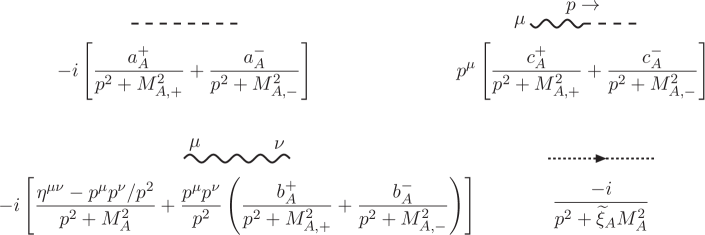
Figure 4.1: Feynman rules for the propagators of the Goldstone scalars $G_{A}$ (dashed lines), massive vectors $Z_{\mu}^{A}$ (wavy lines), and the corresponding ghosts and antighosts $\eta^{A},\overline{\eta}^{A}$ (dotted lines with arrows), each carrying 4-momentum $p^{\mu}$, in the special case that eqs. (4.1) and (4.2) hold. The squared masses $M_{A,\pm}^{2}$ and the coefficients $a_{A}^{\pm}$, $b_{A}^{\pm}$, and $c_{A}^{\pm}$ are defined in eqs. (4.3)-(4.6).

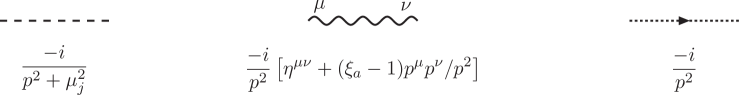
Figure 4.2: Feynman rules for the propagators of the non-Goldstone scalars $R_{j}$ (dashed lines), massless vectors $A_{\mu}^{a}$ (wavy lines), and the corresponding massless ghosts $\overline{\eta}^{a},\eta^{a}$ (dotted lines with arrows), each carrying 4-momentum $p^{\mu}$, in the special case that eqs. (4.1) and (4.2) hold.

The unphysical squared mass poles $M_{\kappa}^{2}$ for the massive vectors and Goldstone scalars are now at

$$M_{A,\pm}^{2} \equiv \widetilde{\xi}_{A}M_{A}^{2}+\frac{1}{2}\biggl{(}\mu_{A}^{2}\pm\sqrt{\mu_{A}^{2}\left[\mu_{A}^{2}+4(\widetilde{\xi}_{A}-\xi_{A})M_{A}^{2}\right]}\biggr{)},$$ (4.3)

for each index $A$, with residue coefficients

$$a_{A}^{\pm} = \frac{M_{A,\pm}^{2}-\xi_{A}M_{A}^{2}}{M_{A,\pm}^{2}-M_{A,\mp}^{2}},$$ (4.4)

$$b_{A}^{\pm} = \frac{(2\xi_{A}-\widetilde{\xi}_{A})\widetilde{\xi}_{A}M_{A}^{2}-\xi_{A}M_{A,\mp}^{2}}{M_{A,\pm}^{2}-M_{A,\mp}^{2}},$$ (4.5)

$$c_{A}^{\pm} = \frac{(\xi_{A}-\widetilde{\xi}_{A})M_{A}}{M_{A,\pm}^{2}-M_{A,\mp}^{2}}.$$ (4.6)

Note that the superscript labels $\pm$ here correspond to the labels $\kappa$ appearing in Figure 2.1, and

$$a_{A}^{+}+a_{A}^{-} = 1,$$ (4.7)

$$b_{A}^{+}+b_{A}^{-} = \xi_{A},$$ (4.8)

$$c_{A}^{+}+c_{A}^{-} = 0.$$ (4.9)

The massive vectors $Z_{\mu}^{A}$ and their associated Goldstone scalars $G_{A}$ have propagator mixing proportional to $\xi_{A}-\widetilde{\xi}_{A}$, and they have three distinct poles in $-p^{2}$, at $M_{A}^{2}$, $M_{A,+}^{2}$, and $M_{A,-}^{2}$. The latter two squared mass poles are real (but not necessarily positive!) if and only if

$$4(\xi_{A}-\widetilde{\xi}_{A})M_{A}^{2}\mu_{A}^{2} \leq (\mu_{A}^{2})^{2}.$$ (4.10)

Note that care is needed to cancel $\mu_{A}^{2}$ in this inequality, because it can have either sign. At one-loop order, complex squared mass poles do not lead to an imaginary part of the effective potential Espinosa:2016uaw , but the two-loop order basis integral $I(x,y,z)$ has a less obvious branch cut structure when one or more of its arguments are complex. In this paper, we will simply avoid choices of the gauge-fixing parameters that make the squared mass arguments complex.

As simple special cases, we have:

Background-field $$R_{\xi} M^{2}_{A,+}=\xi_{A}M_{A}^{2}+\mu_{A}^{2},\>\>\>\>\>\>\>\>M^{2}_{A,-}=M^{2}_{A,\eta}=\xi_{A}M_{A}^{2},$$ gauge: (4.11)

$$a_{A}^{+}=1,\>\>\>\>\>a_{A}^{-}=0,\>\>\>\>\>b_{A}^{+}=0,\>\>\>\>\>b_{A}^{-}=\xi_{A},\>\>\>\>\>c_{A}^{\pm}=0,$$

and the further specialization

Landau gauge: $$M^{2}_{A,+}=\mu_{A}^{2},\>\>\>\>\>\>\>\>\>\>M^{2}_{A,-}=M^{2}_{A,\eta}=0,$$ (4.13)

$$a_{A}^{+}=1,\>\>\>\>\>a_{A}^{-}=0,\>\>\>\>\>b_{A}^{\pm}=0,\>\>\>\>\>c_{A}^{\pm}=0.$$

As before, we use the index of a field as a synonym for the squared mass whenever it appears as the argument of a loop integral function, so that in the following,

$$A = M^{2}_{A},$$ (4.14)

$$A_{\pm} = M^{2}_{A,\pm},$$ (4.15)

$$A_{\eta} = \widetilde{\xi}_{A}M^{2}_{A}.$$ (4.16)

The 1-loop contribution to the effective potential can now be re-expressed as:

$$V^{(1)} = \sum_{j}f(j)-2\sum_{I}f(I)+\sum_{A}\left[3f_{V}(A)+f(A_{+})+f(A_{-})-2f(A_{\eta})\right].$$ (4.17)

In order to facilitate compact expressions below, we also extend the squared-mass notations to the massless vector fields, so that when appearing as the argument of a two-loop integral function, $\bf a$ and ${\bf a}_{\pm}$ and ${\bf a}_{\eta}$ are to be interpreted according to eqs. (4.14)-(4.16) when ${\bf a}=A$, and are taken to vanish when ${\bf a}=a$. We also define residue coefficients

$$b_{a}^{+} = 0,$$ (4.18)

$$b_{a}^{-} = \xi_{a},$$ (4.19)

so that the notation $b_{\bf a}^{\pm}$ is to be interpreted by either eq. (4.5) or eqs. (4.18)-(4.19), depending on whether the corresponding vector field is massive or not. Similarly, for scalar fields, the notation for coefficients $a_{\bf j}^{\pm}$ is to be interpreted using eq. (4.4) when ${\bf j}=A$ is a Goldstone scalar, or

$$a_{j}^{+} = 1,$$ (4.20)

$$a_{j}^{-} = 0,$$ (4.21)

when ${\bf j}=j$ is a non-Goldstone scalar. Furthermore, when ${\bf j}_{\pm}$ appears as an argument in a loop integral function, it is to be interpreted either according to eq. (4.15) for a Goldstone scalar or

$$j_{+} = \mu_{j}^{2},$$ (4.22)

for a non-Goldstone scalar. [Note that $j_{-}$ is not relevant as the argument of a loop integral function, because of eq. (4.21).] The two-loop contributions to the effective potential, given in the most general case in eqs. (3.4)-(3.26), now become:

$$V^{(2)}_{SS} = \frac{1}{8}\lambda^{\bf jjkk}a_{\bf j}^{\epsilon}a_{\bf k}^{\epsilon^{\prime}}f_{SS}({\bf j}_{\epsilon},{\bf k}_{\epsilon^{\prime}}),$$ (4.23)

$$V^{(2)}_{SSS} = \frac{1}{12}\bigl{(}\lambda^{\bf jkl}\bigr{)}^{2}a_{\bf j}^{\epsilon}a_{\bf k}^{\epsilon^{\prime}}a_{\bf l}^{\epsilon^{\prime\prime}}f_{SSS}({\bf j}_{\epsilon},{\bf k}_{\epsilon^{\prime}},{\bf l}_{\epsilon^{\prime\prime}}),$$ (4.24)

$$V^{(2)}_{VS} = \frac{1}{2}\left(g^{\bf a}_{\bf jk}\right)^{2}a_{\bf j}^{\epsilon}\left[f_{VS}({\bf a},{\bf j}_{\epsilon})+b_{\bf a}^{\epsilon^{\prime}}f_{\overline{V}S}({\bf a}_{\epsilon^{\prime}},{\bf j}_{\epsilon})\right],$$ (4.25)

$$V^{(2)}_{SSV} = \frac{1}{4}\left(g^{\bf a}_{\bf jk}\right)^{2}a_{\bf j}^{\epsilon}a_{\bf k}^{\epsilon^{\prime}}\left[f_{SSV}({\bf j}_{\epsilon},{\bf k}_{\epsilon^{\prime}},{\bf a})+b_{\bf a}^{\epsilon^{\prime\prime}}f_{SS\overline{V}}({\bf j}_{\epsilon},{\bf k}_{\epsilon^{\prime}},{\bf a}_{\epsilon^{\prime\prime}})\right],$$ (4.26)

$$V^{(2)}_{VVS} = \frac{1}{4}\bigl{(}G^{\bf ab}_{\bf j}\bigr{)}^{2}a_{\bf j}^{\epsilon}\left[f_{VVS}({\bf a},{\bf b},{\bf j}_{\epsilon})+2b_{\bf a}^{\epsilon^{\prime}}f_{\overline{V}VS}({\bf a}_{\epsilon^{\prime}},{\bf b},{\bf j}_{\epsilon})+b_{\bf a}^{\epsilon^{\prime}}b_{\bf b}^{\epsilon^{\prime\prime}}f_{\overline{V}\overline{V}S}({\bf a}_{\epsilon^{\prime}},{\bf b}_{\epsilon^{\prime\prime}},{\bf j}_{\epsilon})\right],$$ (4.27)

$$V^{(2)}_{SSG} = \frac{1}{2}\lambda^{A\bf jk}g^{A}_{\bf jk}a_{\bf j}^{\epsilon}a_{\bf k}^{\epsilon^{\prime}}c_{A}^{\epsilon^{\prime\prime}}f_{SSG}({\bf j}_{\epsilon},{\bf k}_{\epsilon^{\prime}},A_{\epsilon^{\prime\prime}}),$$ (4.28)

$$V^{(2)}_{GGS} = \frac{1}{2}\lambda^{AB\bf j}G^{AB}_{\bf j}c_{A}^{\epsilon}c_{B}^{\epsilon^{\prime}}a_{\bf j}^{\epsilon^{\prime\prime}}f_{GGS}(A_{\epsilon},B_{\epsilon^{\prime}},{\bf j}_{\epsilon^{\prime\prime}}),$$ (4.29)

$$V^{(2)}_{SGG} = \frac{1}{2}g^{A}_{B\bf j}g^{B}_{A\bf j}a_{\bf j}^{\epsilon}c_{A}^{\epsilon^{\prime}}c_{B}^{\epsilon^{\prime\prime}}f_{SGG}({\bf j}_{\epsilon},A_{\epsilon^{\prime}},B_{\epsilon^{\prime\prime}}),$$ (4.30)

$$V^{(2)}_{GSV} = g^{\bf a}_{{\bf j}A}G^{A\bf a}_{\bf j}c_{A}^{\epsilon}a_{\bf j}^{\epsilon^{\prime}}\left[f_{GSV}(A_{\epsilon},{\bf j}_{\epsilon^{\prime}},{\bf a})+b_{\bf a}^{\epsilon^{\prime\prime}}f_{GS\overline{V}}(A_{\epsilon},{\bf j}_{\epsilon^{\prime}},{\bf a}_{\epsilon^{\prime\prime}})\right],$$ (4.31)

$$V^{(2)}_{GGG} = \frac{1}{2}g^{C}_{AB}G^{AB}_{C}c_{A}^{\epsilon}c_{B}^{\epsilon^{\prime}}c_{C}^{\epsilon^{\prime\prime}}f_{GGG}(A_{\epsilon},B_{\epsilon^{\prime}},C_{\epsilon^{\prime\prime}}),$$ (4.32)

$$V^{(2)}_{GGV} = \frac{1}{2}g^{{\bf a}AB}g^{\bf a}_{AB}c_{A}^{\epsilon}c_{B}^{\epsilon^{\prime}}f_{GGV}(A_{\epsilon},B_{\epsilon^{\prime}},{\bf a}),$$ (4.33)

$$V^{(2)}_{VGG} = \frac{1}{2}G^{A\bf a}_{B}G^{B\bf a}_{A}c_{A}^{\epsilon}c_{B}^{\epsilon^{\prime}}\left[f_{VGG}({\bf a},A_{\epsilon},B_{\epsilon^{\prime}})+b_{\bf a}^{\epsilon^{\prime\prime}}f_{\overline{V}GG}({\bf a}_{\epsilon^{\prime\prime}},A_{\epsilon},B_{\epsilon^{\prime}})\right],$$ (4.34)

$$V^{(2)}_{VVG} = \frac{1}{2}g^{{\bf ab}A}G^{\bf ab}_{A}c_{A}^{\epsilon}\Bigl{[}f_{VVG}({\bf a},{\bf b},A_{\epsilon})+2b_{\bf a}^{\epsilon^{\prime}}f_{\overline{V}VG}({\bf a}_{\epsilon^{\prime}},{\bf b},A_{\epsilon})\Bigr{]},$$ (4.35)

$$V^{(2)}_{\eta\eta S} = \frac{1}{2}g^{A}_{B\bf j}g^{B}_{A\bf j}\widetilde{\xi}_{A}\widetilde{\xi}_{B}M_{A}M_{B}a_{\bf j}^{\epsilon}f_{\eta\eta S}(A_{\eta},B_{\eta},{\bf j}_{\epsilon}),$$ (4.36)

$$V^{(2)}_{\eta\eta G} = g^{{\bf a}AB}g^{\bf a}_{AB}\widetilde{\xi}_{A}M_{A}c_{B}^{\epsilon}f_{\eta\eta G}({\bf a}_{\eta},A_{\eta},B_{\epsilon}),$$ (4.37)

$$V^{(2)}_{VV} = \frac{1}{4}\bigl{(}g^{\bf abc}\bigr{)}^{2}\left[f_{VV}({\bf a},{\bf b})+2b_{\bf a}^{\epsilon}f_{\overline{V}V}({\bf a}_{\epsilon},{\bf b})+b_{\bf a}^{\epsilon}b_{\bf b}^{\epsilon^{\prime}}f_{\overline{V}\overline{V}}({\bf a}_{\epsilon},{\bf b}_{\epsilon^{\prime}})\right],$$ (4.38)

$$V^{(2)}_{VVV} = \frac{1}{12}\bigl{(}g^{\bf abc}\bigr{)}^{2}\Bigl{[}f_{VVV}({\bf a},{\bf b},{\bf c})+3b_{\bf a}^{\epsilon}f_{\overline{V}VV}({\bf a}_{\epsilon},{\bf b},{\bf c})+3b_{\bf a}^{\epsilon}b_{\bf b}^{\epsilon^{\prime}}f_{\overline{V}\overline{V}V}({\bf a}_{\epsilon},{\bf b}_{\epsilon^{\prime}},{\bf c})\Bigr{]},$$ (4.39)

$$V^{(2)}_{\eta\eta V} = \frac{1}{4}\bigl{(}g^{\bf abc}\bigr{)}^{2}\left[f_{\eta\eta V}({\bf a}_{\eta},{\bf b}_{\eta},{\bf c})+b_{\bf c}^{\epsilon}f_{\eta\eta\overline{V}}({\bf a}_{\eta},{\bf b}_{\eta},{\bf c}_{\epsilon})\right],$$ (4.40)

$$V^{(2)}_{FFS} = \frac{1}{2}Y^{{\bf j}IJ}Y_{{\bf j}IJ}a_{\bf j}^{\epsilon}f_{FFS}(I,J,{\bf j}_{\epsilon}),$$ (4.41)

$$V^{(2)}_{\overline{F}\overline{F}S} = \frac{1}{4}(Y^{{\bf j}IJ}Y^{{\bf j}I^{\prime}J^{\prime}}M_{II^{\prime}}M_{JJ^{\prime}}+{\rm c.c.})a_{\bf j}^{\epsilon}f_{\overline{F}\overline{F}S}(I,J,{\bf j}_{\epsilon}),$$ (4.42)

$$V^{(2)}_{FFV} = \frac{1}{2}g^{{\bf a}J}_{I}g^{{\bf a}I}_{J}\left[f_{FFV}(I,J,{\bf a})+b_{\bf a}^{\epsilon}f_{FF\overline{V}}(I,J,{\bf a}_{\epsilon})\right],$$ (4.43)

$$V^{(2)}_{\overline{F}\overline{F}V} = \frac{1}{2}g^{{\bf a}J}_{I}g^{{\bf a}J^{\prime}}_{I^{\prime}}M^{II^{\prime}}M_{JJ^{\prime}}\left[f_{\overline{F}\overline{F}V}(I,J,{\bf a})+b_{\bf a}^{\epsilon}f_{\overline{F}\overline{F}\overline{V}}(I,J,{\bf a}_{\epsilon})\right],$$ (4.44)

$$V^{(2)}_{\overline{F}FG} = i\left(g^{AJ}_{I}Y_{AI^{\prime}J}M^{II^{\prime}}-{\rm c.c.}\right)c_{A}^{\epsilon}f_{\overline{F}FG}(I,J,A_{\epsilon}).$$ (4.45)

In these equations, all indices are summed over in each term that they appear in, including $\epsilon,{\epsilon^{\prime}},{\epsilon^{\prime\prime}}$ each summed over $\pm$.

IV.2 Abelian Higgs model

Consider as an example the Abelian Higgs model. The Lagrangian is:

$${\cal L}=-\frac{1}{4}F^{\mu\nu}F_{\mu\nu}-D^{\mu}\Phi^{*}D_{\mu}\Phi-\Lambda-m^{2}|\Phi|^{2}-\lambda|\Phi|^{4}+{\cal L}_{\rm g.f.}+{\cal L}_{\rm ghosts},$$ (4.46)

where $\Phi$ is a complex scalar field charged under a $U(1)$ gauge symmetry with vector field $Z_{\mu}$ and field strength

$$F_{\mu\nu} = \partial_{\mu}Z_{\nu}-\partial_{\nu}Z_{\mu},$$ (4.47)

with covariant derivatives

$$D_{\mu}\Phi = (\partial_{\mu}-ieZ_{\mu})\Phi,$$ (4.48)

$$D^{\mu}\Phi^{*} = (\partial^{\mu}+ieZ^{\mu})\Phi^{*},$$ (4.49)

and $\lambda$ is a positive scalar self-interaction coupling, $m^{2}$ is a squared mass, and $\Lambda$ is a field-independent vacuum energy (needed for renormalization scale invariance of the effective potential). Now write:

$$\Phi(x) = \frac{1}{\sqrt{2}}[\phi+H(x)+iG(x)],$$ (4.50)

where $\phi$ is the position-independent background scalar field, and $H,G$ are real scalar fields. Then:

$${\cal L} = -\frac{1}{4}F_{\mu\nu}F^{\mu\nu}-\frac{1}{2}(\partial_{\mu}H+eZ_{\mu}G)^{2}-\frac{1}{2}(\partial_{\mu}G-eZ_{\mu}(\phi+H))^{2}$$ (4.51)

$$-\Lambda-\frac{1}{2}m^{2}[G^{2}+(\phi+H)^{2}]-\frac{\lambda}{4}[G^{2}+(\phi+H)^{2}]^{2}$$

$$+{\cal L}_{\rm g.f.}+{\cal L}_{\rm ghost},$$

where, in terms of the Nakanishi-Lautrup Lagrange multiplier field $b$ and the ghost and anti-ghost fields $\eta$ and $\bar{\eta}$,

$${\cal L}_{\rm g.f.} = \frac{1}{2}\xi b^{2}-b(\partial_{\mu}Z^{\mu}-e\widetilde{\xi}\phi G),$$ (4.52)

$${\cal L}_{\rm ghost} = -\partial_{\mu}\bar{\eta}\partial^{\mu}\eta-\widetilde{\xi}e^{2}\phi(\phi+H)\bar{\eta}\eta.$$ (4.53)

This Lagrangian is invariant under the Grassmann-odd BRST symmetry:

$$\delta_{\rm BRST}Z_{\mu} = \partial_{\mu}\eta,$$ (4.54)

$$\delta_{\rm BRST}G = e(\phi+H)\eta,$$ (4.55)

$$\delta_{\rm BRST}H = -eG\eta,$$ (4.56)

$$\delta_{\rm BRST}\bar{\eta} = b,$$ (4.57)

$$\delta_{\rm BRST}\eta = 0,$$ (4.58)

$$\delta_{\rm BRST}b = 0.$$ (4.59)

Because the BRST symmetry does not require any particular relation for $\xi$ and $\widetilde{\xi}$, there is no reason that they should not be renormalized differently, with independent counterterms.

The parameters of the theory are: $\phi$, $e$, $\lambda$, $m^{2}$, $\Lambda$, $\xi$, and $\widetilde{\xi}$. This model can be obtained from the general case by:

$$g_{a} \rightarrow e,$$ (4.60)

$$t^{a}_{GH}=-t^{a}_{HG} = -i,$$ (4.61)

$$g^{a}_{GH}=-g^{a}_{HG} = e,$$ (4.62)

$$\widetilde{\phi}^{a}_{H} = \widetilde{\xi}\phi,$$ (4.63)

$$\widetilde{\phi}^{a}_{G} = 0,$$ (4.64)

$$F^{Z}{}_{G} = e\phi,$$ (4.65)

$$F^{Z}{}_{H} = 0.$$ (4.66)

Because there is only one Goldstone boson and it does not mix with the non-Goldstone scalar $H$, the formalism of the previous subsection IV.1 applies. The squared mass eigenvalues for use as arguments of loop integral functions are:

$$H \equiv m^{2}+3\lambda\phi^{2},$$ (4.67)

$$Z \equiv e^{2}\phi^{2},$$ (4.68)

$$Z_{\pm} \equiv \widetilde{\xi}Z+\frac{1}{2}\left[G\pm\sqrt{G[G+4(\widetilde{\xi}-\xi)Z]}\right],$$ (4.69)

$$\eta \equiv \widetilde{\xi}Z,$$ (4.70)

where

$$G \equiv \mu^{2}_{G}=m^{2}+\lambda\phi^{2}.$$ (4.71)

We also have bosonic propagator residue coefficients:

$$a_{\pm} = \frac{Z_{\pm}-\xi Z}{Z_{\pm}-Z_{\mp}},$$ (4.72)

$$b_{\pm} = \frac{(2\xi-\widetilde{\xi})\widetilde{\xi}Z-\xi Z_{\mp}}{Z_{\pm}-Z_{\mp}},$$ (4.73)

$$c_{\pm} = \frac{(\xi-\widetilde{\xi})e\phi}{Z_{\pm}-Z_{\mp}}.$$ (4.74)

The effective potential in terms of bare parameters can be written as

$$V_{\rm eff} = V^{(0)}_{B}+\frac{1}{16\pi^{2}}V^{(1)}_{B}+\frac{1}{(16\pi^{2})^{2}}V^{(2)}_{B}+\ldots,$$ (4.75)

where the subscript $B$ stands for bare. The tree-level and 1-loop contributions are:

$$V_{B}^{(0)} = \mu^{2\epsilon}\Bigl{(}\Lambda_{B}+\frac{1}{2}m^{2}_{B}\phi^{2}_{B}+\frac{1}{4}\lambda_{B}\phi^{4}_{B}\Bigr{)},$$ (4.76)

$$V_{B}^{(1)} = \Bigl{[}H_{B}{\bf A}(H_{B})+Z_{+,B}{\bf A}(Z_{+,B})+Z_{-,B}{\bf A}(Z_{-,B})-2\eta_{B}{\bf A}(\eta_{B})$$ (4.77)

$$+(3-2\epsilon)Z_{B}{\bf A}(Z_{B})\Bigr{]}/(4-2\epsilon),\phantom{xxx}$$

where $H_{B}$, $Z_{B}$, $Z_{\pm,B}$, and $\eta_{B}$ are obtained from eqs. (4.67)-(4.70) by substituting bare parameters everywhere, and $\epsilon=(4-d)/2$ in $d$ spacetime dimensions, and $\mu$ is the regularization scale (see Appendix A). The 2-loop contributions to the effective potential in the bare scheme can also be obtained from eqs. (4.23)-(4.45), yielding:

$$V^{(2),B}_{SS} = \frac{3\lambda}{4}\Bigl{[}{\bf f}_{SS}(H,H)+a_{+}^{2}{\bf f}_{SS}(Z_{+},Z_{+})+a_{-}^{2}{\bf f}_{SS}(Z_{-},Z_{-})+2a_{+}a_{-}{\bf f}_{SS}(Z_{+},Z_{-})\Bigr{]}$$ (4.78)

$$+\frac{\lambda}{2}\Bigl{[}a_{+}{\bf f}_{SS}(H,Z_{+})+a_{-}{\bf f}_{SS}(H,Z_{-})\Bigr{]},$$

$$V^{(2),B}_{SSS} = \lambda^{2}\phi^{2}\,\bigl{[}3{\bf f}_{SSS}(H,H,H)+a_{+}^{2}{\bf f}_{SSS}(H,Z_{+},Z_{+})$$ (4.79)

$$+a_{-}^{2}{\bf f}_{SSS}(H,Z_{-},Z_{-})+2a_{+}a_{-}{\bf f}_{SSS}(H,Z_{+},Z_{-})\bigr{]},$$

$$V^{(2),B}_{VS} = \frac{e^{2}}{2}\Bigl{[}{\bf f}_{VS}(Z,H)+b_{+}{\bf f}_{\overline{V}S}(Z_{+},H)+b_{-}{\bf f}_{\overline{V}S}(Z_{-},H)$$ (4.80)

$$+a_{+}{\bf f}_{VS}(Z,Z_{+})+a_{-}{\bf f}_{VS}(Z,Z_{-})+a_{+}b_{+}{\bf f}_{\overline{V}S}(Z_{+},Z_{+})$$

$$+a_{-}b_{-}{\bf f}_{\overline{V}S}(Z_{-},Z_{-})+a_{-}b_{+}{\bf f}_{\overline{V}S}(Z_{+},Z_{-})+a_{+}b_{-}{\bf f}_{\overline{V}S}(Z_{-},Z_{+})\Bigr{]},$$

$$V^{(2),B}_{SSV} = \frac{e^{2}}{2}\Bigl{[}a_{+}{\bf f}_{SSV}(H,Z_{+},Z)+a_{-}{\bf f}_{SSV}(H,Z_{-},Z)$$ (4.81)

$$+a_{+}b_{+}{\bf f}_{SS\overline{V}}(H,Z_{+},Z_{+})+a_{-}b_{-}{\bf f}_{SS\overline{V}}(H,Z_{-},Z_{-})$$

$$+a_{+}b_{-}{\bf f}_{SS\overline{V}}(H,Z_{+},Z_{-})+a_{-}b_{+}{\bf f}_{SS\overline{V}}(H,Z_{-},Z_{+})\Bigr{]},$$

$$V^{(2),B}_{VVS} = e^{4}\phi^{2}\Bigl{[}{\bf f}_{VVS}(Z,Z,H)+2b_{+}{\bf f}_{\overline{V}VS}(Z_{+},Z,H)$$ (4.82)

$$+2b_{-}{\bf f}_{\overline{V}VS}(Z_{-},Z,H)+b_{+}^{2}{\bf f}_{\overline{V}\overline{V}S}(Z_{+},Z_{+},H)$$

$$+b_{-}^{2}{\bf f}_{\overline{V}\overline{V}S}(Z_{-},Z_{-},H)+2b_{+}b_{-}{\bf f}_{\overline{V}\overline{V}S}(Z_{+},Z_{-},H)\Bigr{]},$$

$$V^{(2),B}_{SSG} = -2\lambda e\phi\Bigl{[}a_{+}c_{+}{\bf f}_{SSG}(H,Z_{+},Z_{+})+a_{-}c_{-}{\bf f}_{SSG}(H,Z_{-},Z_{-})$$ (4.83)

$$+a_{+}c_{-}{\bf f}_{SSG}(H,Z_{+},Z_{-})+a_{-}c_{+}{\bf f}_{SSG}(H,Z_{-},Z_{+})\Bigr{]},$$

$$V^{(2),B}_{GGS} = 2\lambda e^{2}\phi^{2}\Bigl{[}c_{+}^{2}{\bf f}_{GGS}(Z_{+},Z_{+},H)+c_{-}^{2}{\bf f}_{GGS}(Z_{-},Z_{-},H)$$ (4.84)

$$+2c_{+}c_{-}{\bf f}_{GGS}(Z_{+},Z_{-},H)\Bigr{]},$$

$$V^{(2),B}_{SGG} = \frac{1}{2}e^{2}\Bigl{[}c_{+}^{2}{\bf f}_{SGG}(H,Z_{+},Z_{+})+c_{-}^{2}{\bf f}_{SGG}(H,Z_{-},Z_{-})$$ (4.85)

$$+2c_{+}c_{-}{\bf f}_{SGG}(H,Z_{+},Z_{-})\Bigr{]},$$

$$V^{(2),B}_{GSV} = -2e^{3}\phi\Bigl{[}c_{+}{\bf f}_{GSV}(Z_{+},H,Z)+c_{-}{\bf f}_{GSV}(Z_{-},H,Z)$$ (4.86)

$$+c_{+}b_{+}{\bf f}_{GS\overline{V}}(Z_{+},H,Z_{+})+c_{-}b_{-}{\bf f}_{GS\overline{V}}(Z_{-},H,Z_{-})$$

$$+c_{+}b_{-}{\bf f}_{GS\overline{V}}(Z_{+},H,Z_{-})+c_{-}b_{+}{\bf f}_{GS\overline{V}}(Z_{-},H,Z_{+})\Bigr{]},$$

$$V^{(2),B}_{\eta\eta S} = \frac{1}{2}{\widetilde{\xi}}^{2}e^{4}\phi^{2}{\bf f}_{\eta\eta S}(\eta,\eta,H),$$ (4.87)

where the model-independent integral functions were given above in subsection III.2. There is no need to distinguish between bare and renormalized parameters in the 2-loop part, because the difference is of higher order in the loop expansion.

Now we can derive the $\overline{\rm{MS}}$ version of $V_{\rm eff}$, using an alternative but equivalent method to that described above in the general case. To do so, consider the relationships between bare and $\overline{\rm{MS}}$ parameters:

$$m_{B}^{2} = m^{2}+\frac{1}{16\pi^{2}}\frac{c^{m^{2}}_{1,1}}{\epsilon}++\frac{1}{(16\pi^{2})^{2}}\Bigl{[}\frac{c^{m^{2}}_{2,2}}{\epsilon^{2}}+\frac{c^{m^{2}}_{2,1}}{\epsilon}\Bigr{]}+\ldots,$$ (4.88)

$$\lambda_{B} = \mu^{2\epsilon}\Bigl{(}\lambda+\frac{1}{16\pi^{2}}\frac{c^{\lambda}_{1,1}}{\epsilon}+\frac{1}{(16\pi^{2})^{2}}\Bigl{[}\frac{c^{\lambda}_{2,2}}{\epsilon^{2}}+\frac{c^{\lambda}_{2,1}}{\epsilon}\Bigr{]}+\ldots\Bigr{)},$$ (4.89)

$$\Lambda_{B} = \mu^{-2\epsilon}\Bigl{(}\Lambda+\frac{1}{16\pi^{2}}\frac{c^{\Lambda}_{1,1}}{\epsilon}+\frac{1}{(16\pi^{2})^{2}}\Bigl{[}\frac{c^{\Lambda}_{2,2}}{\epsilon^{2}}+\frac{c^{\Lambda}_{2,1}}{\epsilon}\Bigr{]}+\ldots\Bigr{)},$$ (4.90)

$$e_{B} = \mu^{\epsilon}\Bigl{(}e+\frac{1}{16\pi^{2}}\frac{c^{e}_{1,1}}{\epsilon}+\ldots\Bigr{)},$$ (4.91)

$$\xi_{B} = \xi+\frac{1}{16\pi^{2}}\frac{c^{\xi}_{1,1}}{\epsilon}+\ldots,$$ (4.92)

$$\widetilde{\xi}_{B} = \widetilde{\xi}+\frac{1}{16\pi^{2}}\frac{c^{\widetilde{\xi}}_{1,1}}{\epsilon}+\ldots,$$ (4.93)

$$\phi_{B}^{2} = \mu^{-2\epsilon}\phi^{2}\Bigl{(}1+\frac{1}{16\pi^{2}}\frac{c^{\phi}_{1,1}}{\epsilon}+\frac{1}{(16\pi^{2})^{2}}\Bigl{[}\frac{c^{\phi}_{2,2}}{\epsilon^{2}}+\frac{c^{\phi}_{2,1}}{\epsilon}\Bigr{]}+\ldots\Bigr{)},$$ (4.94)

with counterterm coefficients:

$$c^{m^{2}}_{1,1} = (4\lambda-3e^{2})m^{2},$$ (4.95)

$$c^{m^{2}}_{2,1} = (-10\lambda^{2}+16\lambda e^{2}+43e^{4}/6)m^{2},$$ (4.96)

$$c^{m^{2}}_{2,2} = (28\lambda^{2}-24\lambda e^{2}+10e^{4})m^{2},$$ (4.97)

$$c^{\lambda}_{1,1} = 10\lambda^{2}-6\lambda e^{2}+3e^{4},$$ (4.98)

$$c^{\lambda}_{2,1} = -60\lambda^{3}+28\lambda^{2}e^{2}+79\lambda e^{4}/3-52e^{6}/3,$$ (4.99)

$$c^{\lambda}_{2,2} = 100\lambda^{3}-90\lambda^{2}e^{2}+47\lambda e^{4}-8e^{6},$$ (4.100)

$$c^{\Lambda}_{1,1} = (m^{2})^{2}/2,$$ (4.101)

$$c^{\Lambda}_{2,1} = 2e^{2}(m^{2})^{2},$$ (4.102)

$$c^{\Lambda}_{2,2} = (2\lambda-3e^{2}/2)(m^{2})^{2},$$ (4.103)

$$c^{e}_{1,1} = e^{3}/6,$$ (4.104)

which can be obtained from existing results in the literature MVI ; MVII ; MVIII , and

$$c^{\xi}_{1,1} = -e^{2}\xi/3,$$ (4.105)

$$c^{\widetilde{\xi}}_{1,1} = e^{2}\widetilde{\xi}(\xi-\widetilde{\xi}-10/3),$$ (4.106)

$$c^{\phi}_{1,1} = e^{2}(3-\xi+2\widetilde{\xi}),$$ (4.107)

$$c^{\phi}_{2,1} = -2\lambda^{2}+e^{4}\left(-5/3+\widetilde{\xi}[1+\xi]\right),$$ (4.108)

$$c^{\phi}_{2,2} = e^{4}\left(5-3\xi+\xi^{2}/2+\widetilde{\xi}[3-\xi+\widetilde{\xi}]\right).$$ (4.109)

We obtained eqs. (4.105)-(4.109) by requiring no $1/\epsilon$ or $1/\epsilon^{2}$ poles survive in $V_{\rm eff}$ when written in terms of the $\overline{\rm{MS}}$ parameters. This involves re-expanding $V_{\rm eff}$ from eq. (4.75) both in $1/16\pi^{2}$ and in $\epsilon$ to get the $\overline{\rm{MS}}$ version of the expansion:

$$V_{\rm eff} = V^{(0)}+\frac{1}{16\pi^{2}}V^{(1)}+\frac{1}{(16\pi^{2})^{2}}V^{(2)}+\ldots.$$ (4.110)

The tree-level and 1-loop contributions in the $\overline{\rm{MS}}$ expansion are:

$$V^{(0)} = \Lambda+\frac{1}{2}m^{2}\phi^{2}+\frac{1}{4}\lambda\phi^{4},$$ (4.111)

$$V^{(1)} = f(H)+3f_{V}(Z)+f(Z_{+})+f(Z_{-})-2f(\eta),$$ (4.112)

where $f(x)$ and $f_{V}(x)$ were given in eqs. (3.69) and (3.70) above. The results obtained for the 2-loop $\overline{\rm{MS}}$ contribution $V^{(2)}$ are just given by eqs. (4.78)-(4.87) with each function ${\bf f}$ substituted by the corresponding function $f$ from subsection III.3. Using eqs. (3.108)-(3.127) and then combining the coefficients of basis functions, one obtains:

$$V^{(2)} = \sum_{j}C^{\cal I}_{j}{\cal I}_{j}+\sum_{j,k}C^{\cal AA}_{j,k}{\cal A}_{j}{\cal A}_{k}+\sum_{j}C^{\cal A}_{j}{\cal A}_{j}+C$$ (4.113)

where

$${\cal I} = \{I(H,H,H),\>\>I(H,Z,Z),\>\>I(H,Z,Z_{-}),\>\>I(H,Z,Z_{+}),\>\>I(H,Z_{-},Z_{-}),\>\>$$ (4.114)

$$I(H,Z_{-},Z_{+}),\>\>I(H,Z_{+},Z_{+}),\>\>I(H,\eta,\eta)\},$$

$${\cal A} = \{A(H),\>\>A(Z),\>\>A(Z_{+}),\>\>A(Z_{-})\},$$ (4.115)

and the coefficients $C^{\cal I}_{j}$, $C^{\cal AA}_{j,k}$, $C^{\cal A}_{j}$, and $C$ are rational functions of the $\overline{\rm{MS}}$ parameters of the theory. Although there is significant simplification in the coefficients after combining diagrams, some of them are still somewhat complicated, so the explicit result for $V^{(2)}$ is relegated to an ancillary electronic file V2AH distributed with this paper, in a form suitable for evaluation by computers.

The beta functions of the parameters of the theory in the general form of eq. (1.10), at the orders needed to check renormalization group invariance, are:

$$\beta^{(1)}_{\Lambda} = (m^{2})^{2},$$ (4.116)

$$\beta^{(2)}_{\Lambda} = 8e^{2}(m^{2})^{2},$$ (4.117)

$$\beta^{(1)}_{m^{2}} = (8\lambda-6e^{2})m^{2},$$ (4.118)

$$\beta^{(2)}_{m^{2}} = (86e^{4}/3+64\lambda e^{2}-40\lambda^{2})m^{2},$$ (4.119)

$$\beta^{(1)}_{\lambda} = 6e^{4}-12e^{2}\lambda+20\lambda^{2},$$ (4.120)

$$\beta^{(2)}_{\lambda} = -208e^{6}/3+316e^{4}\lambda/3+112e^{2}\lambda^{2}-240\lambda^{3},$$ (4.121)

$$\beta^{(1)}_{e} = e^{3}/3,$$ (4.122)

$$\beta^{(1)}_{\phi} = (3-\xi+2\widetilde{\xi})e^{2}\phi,$$ (4.123)

$$\beta^{(2)}_{\phi} = [e^{4}(-10/3+2\widetilde{\xi}+2\xi\widetilde{\xi})-4\lambda^{2}]\phi,$$ (4.124)

$$\beta^{(1)}_{\xi} = -2e^{2}\xi/3,$$ (4.125)

$$\beta^{(1)}_{\widetilde{\xi}} = 2e^{2}(\xi-\widetilde{\xi}-10/3)\widetilde{\xi}.$$ (4.126)

These can be obtained from the counterterms provided above.

The background field $R_{\xi}$ gauge-fixing result is obtained by setting $\widetilde{\xi}=\xi$, which simplifies $V^{(2)}$ greatly, resulting in:

$$V^{(2)}_{\widetilde{\xi}=\xi} = \Bigl{\{}[HZ-H^{2}/4-3Z^{2}]I(H,Z,Z)+[(H+Z-G)\eta-\eta^{2}/2-\lambda(G,H,Z)/2]I(H,Z,Z_{+})$$ (4.127)

$$-[(H-G)^{2}/4]I(H,Z_{+},Z_{+})+[(H+\eta-Z)^{2}/2-2\eta H]I(H,Z,\eta)$$

$$+[(H-Z_{+})^{2}/2]I(H,\eta,Z_{+})+[\eta H-\eta^{2}/2-H^{2}/4]I(H,\eta,\eta)-[3(H-G)^{2}/4]I(H,H,H)$$

$$+[H/4-Z/2]A(Z)^{2}+[H/4-\eta/2]A(\eta)^{2}+[3(H-G)/8]A(Z_{+})^{2}$$

$$+[3(H-G)/8]A(H)^{2}+[(H+2Z-\eta-G)/2]A(Z)A(Z_{+})+[(Z_{+}-H)/2]A(\eta)A(Z_{+})$$

$$+[(Z+\eta-H)/2]A(Z)A(\eta)+[(3Z-H+G)/2]A(H)A(Z)$$

$$+[(H+2Z-G)/4]A(H)A(Z_{+})+[(H-Z-G)/2]A(H)A(\eta)$$

$$+Z[G+H+2Z/3]A(Z)+3Z^{2}A(H)+Z^{2}A(Z_{+})-Z^{2}(2Z+H)\Bigr{\}}/\phi^{2},$$

where now $Z_{-}=\eta=\xi Z$ and $Z_{+}=\eta+G$. This gauge has the nice property that all squared mass arguments are real and positive as long as $\xi$ is positive with $\xi Z>-G$, in which case there are no infrared problems for small $G$. However, as noted above, this gauge-fixing condition is not respected by renormalization, as can be seen from eqs. (4.125) and (4.126), which clearly do not preserve $\xi=\widetilde{\xi}$ if imposed as an initial condition. Moreover, if the $\overline{\rm{MS}}$ gauge fixing parameters obey $\xi=\widetilde{\xi}$ at some particular choice of renormalization scale, then the corresponding bare parameters will not obey this condition.

IV.3 The Standard Model

In this section we obtain the Standard Model results as a special case of the results above. The parameters of the theory consist of the constant background Higgs scalar field $\phi$, a field-independent vacuum energy $\Lambda$, a Higgs scalar squared mass parameter $m^{2}$, a Higgs self-interaction coupling $\lambda$, gauge couplings $g_{3},g,g^{\prime}$, the top-quark Yukawa coupling $y_{t}$, and gauge-fixing parameters $\xi_{\gamma}$, $\xi_{Z}$, $\widetilde{\xi}_{Z}$, $\xi_{W}$, $\widetilde{\xi}_{W}$. The 2-loop effective potential does depend on the QED gauge-fixing parameter $\xi_{\gamma}$, but not on the corresponding QCD $SU(3)_{c}$ gauge-fixing parameter $\xi_{QCD}$. There is no parameter $\widetilde{\xi}_{\gamma}$, because the photon is massless. The Yukawa couplings of all fermions other than the top quark are negligible, and neglected.

The field content with $n_{G}$ generations consists of:

Real vectors: $$A,Z,W_{R},W_{I},$$ (4.128)

Real scalars: $$H,G_{0},G_{I},G_{R},$$ (4.129)

2-component fermions: $$t,\,\bar{t},\,b,\,\bar{b},\,\tau,\,\bar{\tau},\,\nu_{\tau}\>+\>(n_{G}-1)\times\left(u,\,\bar{u},\,d,\,\bar{d},\,e,\,\bar{e},\,\nu_{e}\right),\phantom{xxxx}$$ (4.130)

and the color octet gluons, which do not pose any problems with respect to gauge fixing. The charged $W$ bosons and charged Goldstone scalars have been split into real and imaginary parts $W_{R}$, $W_{I}$ and $G_{R}$, $G_{I}$ respectively. We now list all of the (non-QCD) interactions of the Standard Model.

The scalar cubic interactions are

$$\lambda^{HHH} = 6\lambda\phi,$$ (4.131)

$$\lambda^{HG_{0}G_{0}} = \lambda^{HG_{R}G_{R}}\>=\>\lambda^{HG_{I}G_{I}}\>=\>2\lambda\phi,$$ (4.132)

and the scalar quartic couplings are

$$\lambda^{HHHH} = \lambda^{G_{0}G_{0}G_{0}G_{0}}\>=\>\lambda^{G_{R}G_{R}G_{R}G_{R}}\>=\>\lambda^{G_{I}G_{I}G_{I}G_{I}}\>=\>6\lambda,$$ (4.133)

$$\lambda^{HHG_{0}G_{0}} = \lambda^{HHG_{R}G_{R}}=\lambda^{HHG_{I}G_{I}}=\lambda^{G_{0}G_{0}G_{R}G_{R}}=\lambda^{G_{0}G_{0}G_{I}G_{I}}=\lambda^{G_{R}G_{R}G_{I}G_{I}}=2\lambda,\phantom{xxx}$$ (4.134)

with both of these lists supplemented by all cases dictated by the symmetry under interchange of any two scalars. The Yukawa couplings (neglecting all fermion mass effects other than the top quark) are given by

$$Y^{Ht\bar{t}}=-Y^{G_{R}b\bar{t}}=iY^{G_{0}t\bar{t}}=iY^{G_{I}b\bar{t}} = y_{t}/\sqrt{2},$$ (4.135)

with symmetry under interchange of the fermion (last two) indices. The electroweak gauge boson interactions with the fermions are given by couplings of the type $g^{{\bf a}J}_{I}$:

$$g^{Zf}_{f} = I_{f}gc_{W}-Y_{f}g^{\prime}s_{W},$$ (4.136)

$$g^{Z\bar{f}}_{\bar{f}} = Q_{f}g^{\prime}s_{W},$$ (4.137)

$$g^{Af}_{f} = -g^{A\bar{f}}_{\bar{f}}=Q_{f}e,$$ (4.138)

where

$$e = gg^{\prime}/\sqrt{g^{2}+g^{\prime 2}},$$ (4.139)

$$s_{W} = g^{\prime}/\sqrt{g^{2}+g^{\prime 2}},$$ (4.140)

$$c_{W} = g/\sqrt{g^{2}+g^{\prime 2}},$$ (4.141)

and $Q_{u}=2/3$ and $Q_{d}=-1/3$ and $Q_{\nu}=0$ and $Q_{e}=-1$, and $I_{u}=I_{\nu}=1/2$ and $I_{d}=I_{e}=-1/2$, and $Y_{f}=Q_{f}-I_{f}$ for each $f$, and

$$g^{W_{R}u}_{d}=g^{W_{R}d}_{u}=g^{W_{R}\nu}_{e}=g^{W_{R}e}_{\nu}=g/2,$$ (4.142)

$$g^{W_{I}u}_{d}=-g^{W_{I}d}_{u}=g^{W_{I}\nu}_{e}=-g^{W_{I}e}_{\nu}=ig/2.$$ (4.143)

The non-zero vector-scalar-scalar interaction couplings of the type $g^{\bf a}_{\bf jk}$ are

$$g^{A}_{G_{I}G_{R}} = e,$$ (4.144)

$$g^{Z}_{G_{0}H} = \sqrt{g^{2}+g^{\prime 2}}/2,$$ (4.145)

$$g^{Z}_{G_{I}G_{R}} = (g^{2}-g^{\prime 2})/(2\sqrt{g^{2}+g^{\prime 2}}),$$ (4.146)

$$g^{W_{R}}_{G_{R}G_{0}} = g^{W_{R}}_{G_{I}H}\>=\>g^{W_{I}}_{G_{0}G_{I}}\>=\>g^{W_{I}}_{G_{R}H}\>=\>g/2,$$ (4.147)

with antisymmetry under interchange of the scalar (lowered) indices. The vector-vector-scalar-scalar interactions are determined in terms of these [see eq. (2.28) and fig. 2.4], and so there is no need to list them separately. The non-zero vector-vector-scalar couplings of the type $G^{\bf ab}_{\bf j}$ follow from eqs. (2.31)-(2.33), and are given by:

$$G^{AW_{R}}_{G_{R}}\>=\>-G^{AW_{I}}_{G_{I}} = ge\phi/2,$$ (4.148)

$$G^{ZW_{I}}_{G_{I}}\>=\>-G^{ZW_{R}}_{G_{R}} = g^{\prime}e\phi/2,$$ (4.149)

$$G^{W_{R}W_{R}}_{H}\>=\>G^{W_{I}W_{I}}_{H} = g^{2}\phi/2,$$ (4.150)

$$G^{ZZ}_{H} = (g^{2}+g^{\prime 2})\phi/2,$$ (4.151)

and others determined by symmetry under interchanging the vector (raised) indices. Finally there are the totally anti-symmetric vector-vector-vector couplings defined by:

$$g^{AW_{R}W_{I}} = e,$$ (4.152)

$$g^{ZW_{R}W_{I}} = g^{2}/\sqrt{g^{2}+g^{\prime 2}}.$$ (4.153)

The matrix $F^{\bf a}{}_{\bf j}$ of gauge boson masses, using the ordered bases $(W_{R},W_{I},Z,A)$ and $(G_{I},G_{R},G_{0},H)$, is diagonal, and positive in the convention chosen here when $\phi$ is positive, with non-zero entries:

$$F^{W_{R}}{}_{G_{I}}=F^{W_{I}}{}_{G_{R}} = M_{W}=g\phi/2,$$ (4.154)

$$F^{Z}{}_{G_{0}} = M_{Z}=\sqrt{g^{2}+g^{\prime 2}}\phi/2.$$ (4.155)

The gauge-fixing part of the Lagrangian is:

$${\cal L} = -\frac{1}{2\xi_{\gamma}}(\partial_{\mu}A^{\mu})^{2}-\frac{1}{2\xi_{Z}}(\partial_{\mu}Z^{\mu}-\widetilde{\xi}_{Z}M_{Z}G_{0})^{2}$$ (4.156)

$$-\frac{1}{2\xi_{W}}(\partial_{\mu}W_{R}^{\mu}-\widetilde{\xi}_{W}M_{W}G_{I})^{2}-\frac{1}{2\xi_{W}}(\partial_{\mu}W_{I}^{\mu}-\widetilde{\xi}_{W}M_{W}G_{R})^{2}.$$

As an aside, we note that our choice of basis for the gauge-fixing terms differs from the choice made in ref. DiLuzio:2014bua , in which the neutral bosons have a gauge fixing Lagrangian that is instead equivalent to the form:

$$-\frac{1}{2\xi_{1}}(\partial_{\mu}B^{\mu}-\widetilde{\xi}_{1}M_{B}G_{0})^{2}-\frac{1}{2\xi_{2}}(\partial_{\mu}W_{0}^{\mu}-\widetilde{\xi}_{2}M_{W}G_{0})^{2}$$ (4.157)

where $M_{B}=g^{\prime}\phi/2$ and $B^{\mu}=c_{W}A^{\mu}-s_{W}Z^{\mu}$ and $W_{0}^{\mu}=c_{W}Z^{\mu}+s_{W}A^{\mu}$ are the gauge-eigenstate neutral vector fields for $U(1)_{Y}$ and $SU(2)_{L}$ respectively. Note that there is no redefinition of gauge-fixing parameters that can make this choice equivalent to ours in general, because the cross-terms are different; in particular, eq. (4.157) implies a mixing between the photon and the $Z$ boson (unless $\xi_{1}=\xi_{2}$) and between the photon and the neutral Goldstone boson (unless $\xi_{1}\widetilde{\xi}_{2}=-\xi_{2}\widetilde{\xi}_{1}$). We prefer our choice of a mass-eigenstate basis for the gauge fixing terms because it avoids this tree-level gauge-dependent mixing of the photon. This inequivalence illustrates the general remark made just before eq. (2.13) above, concerning the fact that the form of the gauge-fixing terms depends on the choice of basis. (The equivalence could be restored if the gauge fixing parameter $\xi_{\bf a}$ were generalized to a matrix $\xi_{\bf ab}$.)

The squared mass poles associated with the electroweak bosons and their ghosts are at 0 and

$$H = m^{2}+3\lambda\phi^{2},$$ (4.158)

$$Z = (g^{2}+g^{\prime 2})\phi^{2}/4,$$ (4.159)

$$Z_{\pm} = \widetilde{\xi}_{Z}Z+\frac{1}{2}\left[G\pm\sqrt{G[G+4(\widetilde{\xi}_{Z}-\xi_{Z})Z]}\right],$$ (4.160)

$$\eta_{Z} = \widetilde{\xi}_{Z}Z,$$ (4.161)

$$W = g^{2}\phi^{2}/4,$$ (4.162)

$$W_{\pm} = \widetilde{\xi}_{W}W+\frac{1}{2}\left[G\pm\sqrt{G[G+4(\widetilde{\xi}_{W}-\xi_{W})W]}\right],$$ (4.163)

$$\eta_{W} = \widetilde{\xi}_{W}W,$$ (4.164)

where

$$G=m^{2}+\lambda\phi^{2},$$ (4.165)

which coincides the Landau gauge version of the common Goldstone squared mass. The only other non-zero squared mass is that of the top quark,

$$T=y_{t}^{2}\phi^{2}/2.$$ (4.166)

Because there is no mixing among the Goldstone bosons or between them and $H$, the results of subsection IV.1 apply. Using those results, and combining coefficients of basis functions, the tree-level and one-loop results for the Standard Model in the $\overline{\rm{MS}}$ scheme are

$$V^{(0)} = \Lambda+m^{2}\phi^{2}/2+\lambda\phi^{4}/4,$$ (4.167)

$$V^{(1)} = f(H)-12f(T)+6f_{V}(W)+2f(W_{+})+2f(W_{-})-4f(\eta_{W})$$ (4.168)

$$+3f_{V}(Z)+f(Z_{+})+f(Z_{-})-2f(\eta_{Z}),$$

and, using eqs. (3.108)-(3.172), the two-loop part $V^{(2)}$ can be written in the same form as eq. (4.113), but now with:

$${\cal A} = \{A(H),\>A(t),\>A(W),\>A(W_{+}),\>A(W_{-}),\>A(\eta_{W}),\>A(Z),\>A(Z_{+}),\>A(Z_{-}),\>A(\eta_{Z})\},\phantom{xx}$$ (4.169)

and

$${\cal I} = \{I(H,T,T),\>\>I(T,T,Z),\>\>I(T,T,Z_{-}),\>\>I(T,T,Z_{+}),\>\>I(0,T,W),\>\>I(0,T,W_{-}),\>\>$$ (4.170)

$$I(0,T,W_{+}),\>\>I(0,0,W),\>\>I(0,0,Z),\>\>I(0,W,W_{-}),\>\>I(0,W,W_{+}),\>\>I(0,W_{-},W_{+}),\>\>$$

$$I(0,\eta_{W},W),\>\>I(0,\eta_{W},W_{-}),\>\>I(0,\eta_{W},W_{+}),\>\>I(H,H,H),\>\>I(H,W,W),\>\>$$

$$I(H,W,W_{-}),\>\>I(H,W,W_{+}),\>\>I(H,W_{-},W_{-}),\>\>I(H,W_{-},W_{+}),\>\>I(H,W_{+},W_{+}),\>\>$$

$$I(H,\eta_{W},\eta_{W}),\>\>I(H,Z,Z),\>\>I(H,Z,Z_{-}),\>\>I(H,Z,Z_{+}),\>\>I(H,Z_{-},Z_{-}),\>\>I(H,Z_{-},Z_{+}),\>\>$$

$$I(H,Z_{+},Z_{+}),\>\>I(H,\eta_{Z},\eta_{Z}),\>\>I(W,W,Z),\>\>I(W,W_{-},Z),\>\>I(W,W_{-},Z_{-}),\>\>I(W,W_{-},Z_{+}),\>\>$$

$$I(W,W_{+},Z),\>\>I(W,W_{+},Z_{-}),\>\>I(W,W_{+},Z_{+}),\>\>I(W_{-},W_{-},Z),\>\>I(W_{-},W_{+},Z),\>\>$$

$$I(W_{-},W_{+},Z_{-}),\>\>I(W_{-},W_{+},Z_{+}),\>\>I(W_{+},W_{+},Z),\>\>I(\eta_{W},\eta_{Z},W),\>\>I(\eta_{W},\eta_{W},Z),\>\>$$

$$I(\eta_{W},\eta_{W},Z_{-}),\>\>I(\eta_{W},\eta_{W},Z_{+}),\>\>I(\eta_{W},\eta_{Z},W_{-}),\>\>I(\eta_{W},\eta_{Z},W_{+})\}.$$

The coefficients in this result for $V^{(2)}$ are rather complicated, so they are again relegated to an electronic ancillary file V2SM distributed with this paper, in a form suitable for evaluation by computers. For convenience, we also include separate files V2SMFermi and V2SMbackgroundRxi and V2SMLandau for the specializations to Fermi gauges (with $\widetilde{\xi}_{Z}=\widetilde{\xi}_{W}=0$) and to background field $R_{\xi}$ gauges (with $\widetilde{\xi}_{Z}=\xi_{Z}$ and $\widetilde{\xi}_{W}=\xi_{W}$) and Landau gauge (with $\xi_{A}=\widetilde{\xi}_{Z}=\xi_{Z}=\widetilde{\xi}_{W}=\xi_{W}=0$), respectively.

The check of renormalization group invariance of the effective potential can now be carried out as in eq. (1.12), with the beta functions:

$$\beta_{\Lambda}^{(1)} = 2(m^{2})^{2},$$ (4.171)

$$\beta_{\Lambda}^{(2)} = (12g^{2}+4g^{\prime 2}-12y_{t}^{2})(m^{2})^{2},$$ (4.172)

$$\beta_{m^{2}}^{(1)} = m^{2}(6y_{t}^{2}+12\lambda-9g^{2}/2-3g^{\prime 2}/2),$$ (4.173)

$$\beta_{m^{2}}^{(2)} = m^{2}(40g_{3}^{2}y_{t}^{2}-27y_{t}^{4}/2+45y_{t}^{2}g^{2}/4+85y_{t}^{2}g^{\prime 2}/12-72y_{t}^{2}\lambda+(5n_{G}-385/16)g^{4}$$ (4.174)

$$+15g^{2}g^{\prime 2}/8+(25n_{G}/9+157/48)g^{\prime 4}+72g^{2}\lambda+24g^{\prime 2}\lambda-60\lambda^{2}),$$

$$\beta_{\lambda}^{(1)} = -6y_{t}^{4}+12y_{t}^{2}\lambda+9g^{4}/8+3g^{2}g^{\prime 2}/4+3g^{\prime 4}/8-9g^{2}\lambda-3g^{\prime 2}\lambda+24\lambda^{2},$$ (4.175)

$$\beta_{\lambda}^{(2)} = -32g_{3}^{2}y_{t}^{4}+80g_{3}^{2}y_{t}^{2}\lambda+30y_{t}^{6}-8y_{t}^{4}g^{\prime 2}/3-3y_{t}^{4}\lambda-9y_{t}^{2}g^{4}/4+21y_{t}^{2}g^{2}g^{\prime 2}/2$$ (4.176)

$$-19y_{t}^{2}g^{\prime 4}/4+45y_{t}^{2}g^{2}\lambda/2+85y_{t}^{2}g^{\prime 2}\lambda/6-144y_{t}^{2}\lambda^{2}+(497/16-4n_{G})g^{6}$$

$$-(97/48+4n_{G}/3)g^{4}g^{\prime 2}-(239/48+20n_{G}/9)g^{2}g^{\prime 4}-(59/48+20n_{G}/9)g^{\prime 6}$$

$$+(10n_{G}-313/8)g^{4}\lambda+39g^{2}g^{\prime 2}\lambda/4+(229/24+50n_{G}/9)g^{\prime 4}\lambda+108g^{2}\lambda^{2}$$

$$+36g^{\prime 2}\lambda^{2}-312\lambda^{3},$$

$$\beta_{g^{\prime}}^{(1)} = (20n_{G}/9+1/6)g^{\prime 3},$$ (4.177)

$$\beta_{g}^{(1)} = (4n_{G}/3-43/6)g^{3},$$ (4.178)

$$\beta^{(1)}_{\phi} = \bigl{[}-3y_{t}^{2}+9g^{2}/4+3g^{\prime 2}/4+(\widetilde{\xi}_{W}-\xi_{W}/2)g^{2}+(\widetilde{\xi}_{Z}/2-\xi_{Z}/4)(g^{2}+g^{\prime 2})\bigr{]}\phi,$$ (4.179)

$$\beta^{(2)}_{\phi} = \bigl{\{}y_{t}^{2}[27y_{t}^{2}/4-20g_{3}^{2}-45g^{2}/8-85g^{\prime 2}/24]-6\lambda^{2}$$ (4.180)

$$+(511/32-5n_{G}/2)g^{4}-9g^{2}g^{\prime 2}/16-(25n_{G}/18+31/96)g^{\prime 4}$$

$$-3y_{t}^{2}[\widetilde{\xi}_{W}g^{2}+\widetilde{\xi}_{Z}(g^{2}+g^{\prime 2})/2]+\xi_{W}[(\widetilde{\xi}_{W}/4-2-\xi_{W}/8-\xi_{Z}/4)g^{4}+\widetilde{\xi}_{Z}g^{2}g^{\prime 2}/4]$$

$$+\xi_{\gamma}(\widetilde{\xi}_{W}-3)e^{2}g^{2}/4+\xi_{Z}[-g^{4}c_{W}^{2}-e^{2}g^{2}/4+\widetilde{\xi}_{W}e^{2}g^{\prime 2}/4+\widetilde{\xi}_{Z}(g^{2}+g^{\prime 2})^{2}/8]$$

$$+\widetilde{\xi}_{W}(17g^{4}+g^{2}g^{\prime 2})/4+\widetilde{\xi}_{Z}(17g^{4}+4g^{2}g^{\prime 2}+g^{\prime 4})/8\bigr{\}}\phi,$$

$$\beta_{\xi_{W}}^{(1)} = \xi_{W}g^{2}\left[25/3-8n_{G}/3-\xi_{W}-c_{W}^{2}\xi_{Z}-s_{W}^{2}\xi_{\gamma}\right],$$ (4.181)

$$\beta_{\widetilde{\xi}_{W}}^{(1)} = \widetilde{\xi}_{W}\bigl{[}6y_{t}^{2}+(41/6-8n_{G}/3)g^{2}-3g^{\prime 2}/2+\xi_{\gamma}e^{2}/2+(\xi_{W}/2-\widetilde{\xi}_{W})g^{2}$$ (4.182)

$$+\xi_{Z}g^{\prime 2}s_{W}^{2}/2-\widetilde{\xi}_{Z}(g^{2}+g^{\prime 2})/2\bigr{]},$$

$$\beta_{\xi_{Z}}^{(1)} = \xi_{Z}\left[g^{2}c_{W}^{2}(25/3-8n_{G}/3-2\xi_{W})-g^{\prime 2}s_{W}^{2}(1/3+40n_{G}/9)\right],$$ (4.183)

$$\beta_{\widetilde{\xi}_{Z}}^{(1)} = \widetilde{\xi}_{Z}\bigl{[}6y_{t}^{2}+(41/6-8n_{G}/3)g^{2}c_{W}^{2}-(11/6+40n_{G}/9)g^{\prime 2}s_{W}^{2}-6e^{2}+\xi_{W}e^{2}$$ (4.184)

$$-\widetilde{\xi}_{W}g^{2}+(\xi_{Z}-\widetilde{\xi}_{Z})(g^{2}+g^{\prime 2})/2\bigr{]}$$

$$\beta_{\xi_{\gamma}}^{(1)} = \xi_{\gamma}e^{2}\left[8-64n_{G}/9-2\xi_{W}\right].$$ (4.185)

Equations (4.171) and (4.172) were obtained in ref. Martin:2017lqn , and eqs. (4.173)-(4.178) and the parts of eqs. (4.179) and (4.180) that do not depend on the gauge-fixing parameters $\xi_{W}$, $\xi_{Z}$, $\widetilde{\xi}_{W}$, $\widetilde{\xi}_{Z}$ can be found in the literature, for example in refs. MVI -MVIII . The results dependent on the gauge-fixing parameters in eqs. (4.179)-(4.184) were obtained here by requiring that $V_{\rm eff}$ satisfies renormalization group invariance. Again we note that any equality among any subset of the parameters $\xi_{W}$, $\xi_{Z}$, $\widetilde{\xi}_{W}$, $\widetilde{\xi}_{Z}$, and $\xi_{\gamma}$ will not be preserved under renormalization group evolution, except in the special case that the corresponding parameters vanish. Also, if the $\overline{\rm{MS}}$ gauge fixing parameters obey $\xi_{W}=\widetilde{\xi}_{W}$ and/or $\xi_{Z}=\widetilde{\xi}_{Z}$ at some particular choice of renormalization scale, then the corresponding bare parameters will not obey these conditions, and vice versa.

V Numerical results for the Standard Model

Consider the Standard Model with the following input parameters as a benchmark (the same as in refs. Martin:2015lxa ; Martin:2015rea ; Martin:2016xsp ; Martin:2015eia ; Martin:2017lqn , but with various other approximations for the effective potential):

$$Q = M_{t}=173.34\>\mbox{GeV},$$ (5.1)

$$y_{t}(Q) = 0.93690,$$ (5.2)

$$g_{3}(Q) = 1.1666,$$ (5.3)

$$g(Q) = 0.647550,$$ (5.4)

$$g^{\prime}(Q) = 0.358521,$$ (5.5)

$$\lambda(Q) = 0.12597,$$ (5.6)

$$m^{2}(Q) = -(92.890\>\mbox{GeV})^{2}$$ (5.7)

$$\Lambda(Q) = 0.$$ (5.8)

Then, in the Landau gauge, the minimum of the (real part of the) 2-loop effective potential is at

$$v_{0}\equiv\phi_{\rm min}^{(\xi=0)} = 246.950\>\mbox{GeV},$$ (5.9)

$$V_{\rm eff}^{(\xi=0)}(v_{0}) = -(105.560\>\mbox{GeV})^{4}.$$ (5.10)

With this choice of input parameters, the Landau gauge Goldstone boson $\overline{\rm{MS}}$ squared mass is $G=-(\mbox{30.763 GeV})^{2}$, so that $V_{\rm eff}$ is actually complex at its minimum. For simplicity we do not apply the Goldstone boson resummation procedure Martin:2014bca ; Elias-Miro:2014pca to eliminate the spurious imaginary part here. Instead, we simply minimize the real part of $V_{\rm eff}$, and it should be understood below that the spurious imaginary part is always dropped. As shown in ref. Martin:2014bca , the practical numerical difference between the VEV obtained by minimizing the real part of the non-resummed effective potential and the VEV obtained by minimizing the Goldstone boson-resummed effective potential, which is always real, is very small.

In Figure 5.1, we show the results for $v=\phi_{\rm min}$ and $V_{\rm eff}(v)$ as a function of $\xi$ for the cases:

$$\mbox{background field $R_{\xi}$ gauge}: \xi\equiv\xi_{W}=\widetilde{\xi}_{W}=\xi_{Z}=\widetilde{\xi}_{Z}=\xi_{\gamma},$$ (5.11)

$$\mbox{Fermi gauges}: \xi\equiv\xi_{W}=\xi_{Z}=\xi_{\gamma},\quad\mbox{and}\quad\widetilde{\xi}_{W}=\widetilde{\xi}_{Z}=0.$$ (5.12)

In the background field $R_{\xi}$ gauge, for small $\xi$ one finds that $M^{2}_{Z,+}$ and $M^{2}_{W,+}$ are negative and so $V_{\rm eff}(v)$ has a spurious imaginary part, but $M^{2}_{Z,+}$ becomes positive for $\xi>0.11112$, and $M^{2}_{W,+}$ is positive for $\xi>0.14388$, so that there is no spurious imaginary part at the minimum of the two-loop effective potential for $\xi$ larger than this. (Very small cusps are visible on the background field $R_{\xi}$ gauge curve for $v$, corresponding to the points where $M^{2}_{Z,+}$ and $M^{2}_{W,+}$ go through 0.) In the Fermi gauge, $M^{2}_{Z,+}$ and $M^{2}_{W,+}$ are positive but $M^{2}_{Z,-}$ and $M^{2}_{W,-}$ are negative for all positive $\xi$, so that the effective potential always has a spurious imaginary part, which again is ignored in the minimization.

Although $v$ is a non-trivial function of $\xi$, the minimum vacuum energy $V_{\rm eff}(v)$ is a physical observable (for example, by weakly coupling to gravity) and in principle should be completely independent of $\xi$ when computed to all orders in perturbation theory. In the second panel of Figure 5.1, it can be seen that the latter property indeed holds in the background field $R_{\xi}$ gauge to better than 1 part per mille for $\xi\mathrel{\hbox to0.0pt{\lower 4.0pt\hbox{$\sim$}\hss}\raise 1.0pt\hbox{$<$}}16$ and to better than 1% for $\xi\mathrel{\hbox to0.0pt{\lower 4.0pt\hbox{$\sim$}\hss}\raise 1.0pt\hbox{$<$}}37$, but the situation rapidly deteriorates for larger $\xi$. In Fermi gauge, the deviation is larger, but $V_{\rm eff}(v)$ differs from its Landau gauge value by less than 1 part per mille for all $\xi\mathrel{\hbox to0.0pt{\lower 4.0pt\hbox{$\sim$}\hss}\raise 1.0pt\hbox{$<$}}1.88$ and by less than 1% for $\xi\mathrel{\hbox to0.0pt{\lower 4.0pt\hbox{$\sim$}\hss}\raise 1.0pt\hbox{$<$}}14$; the deviation again grows rapidly for larger $\xi$. In the second panel of Figure 5.1 the results from the 1-loop effective potential approximations are also shown, as dashed lines; the deviations are significantly worse than at 2-loop order.

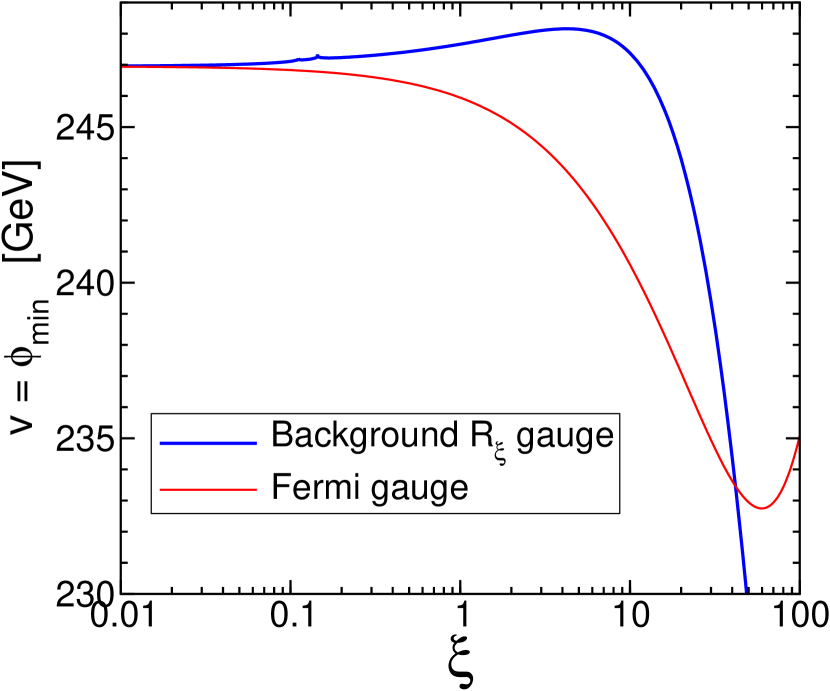
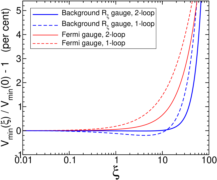
Figure 5.1: The Higgs VEV (top panel), and the resulting fractional change in the vacuum energy compared to the Landau gauge $\xi=0$ result, in per cent (bottom panel), at the minimum of the 2-loop Standard Model effective potential, as a function of the gauge-fixing parameter $\xi$. The solid blue (thicker) curves show the result for the background field $R_{\xi}$ gauges (with $\xi\equiv\xi_{W}=\widetilde{\xi}_{W}=\xi_{Z}=\widetilde{\xi}_{Z}=\xi_{\gamma}$), and the solid red (thinner) curves are the results for the Fermi gauges (with $\xi\equiv\xi_{W}=\xi_{Z}=\xi_{\gamma}$ and $\widetilde{\xi}_{W}=\widetilde{\xi}_{Z}=0$.) The other input parameters are as given in eqs. (5.1)-(5.8) of the text. In the top panel, very small cusps are barely visible in the background field $R_{\xi}$ gauge $v$ curve at the points $\xi=0.11112$ and $0.14388$ below which $M^{2}_{Z,+}$ and $M^{2}_{W,+}$, respectively, are negative. In the bottom panel, we also show for comparison the results from the 1-loop approximations, as dashed lines. The dependence of the VEV on $\xi$ is expected, but in principle the minimum value of the vacuum energy is an observable and should be independent of $\xi$. The significant deviation from this idealized behavior shown in the bottom panel is due to a breakdown in perturbation theory truncated at 2-loop order for large $\xi$.

In Figure 5.2, we show results for the background field $R_{\xi}$ gauge for seven different choices of the renormalization scale $Q$. In each case we show the deviation of $V_{\rm eff,min}(\xi,Q)$ compared to the benchmark value $V_{\rm eff,min}(0,M_{t})$ obtained in Landau gauge and with $Q$ set equal to $M_{t}=173.34$ GeV. To make this graph, the parameters in eqs. (5.1)-(5.8) are first run according to their 2-loop renormalization group equations to the scale $Q$, and then the minimum value of the two-loop effective potential $V_{\rm eff,min}(\xi,Q)$ is obtained. Since $V_{\rm eff,min}(\xi,Q)$ is a physical observable, it should in principle be independent of both $\xi$ and $Q$ if calculated to all orders. We see that for $\xi$ less than of order roughly 30, in the 2-loop approximation the dependence on $\xi$ is much smaller than the dependence on the renormalization scale, but for larger $\xi$ this is no longer true as perturbation theory breaks down.

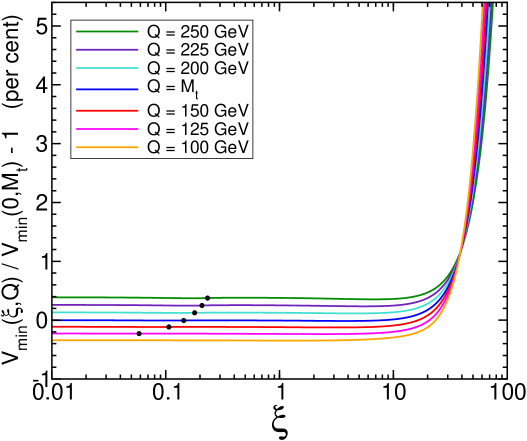
Figure 5.2: The fractional change in the vacuum energy in per cent, at the minimum of the 2-loop Standard Model effective potential, as a function of the background $R_{\xi}$ gauge-fixing parameter $\xi\equiv\xi_{W}=\widetilde{\xi}_{W}=\xi_{Z}=\widetilde{\xi}_{Z}=\xi_{\gamma}$. The comparison value $V_{\rm min}(0,M_{t})$ is the Landau gauge result with the input parameters of eqs. (5.1)-(5.8) at $Q=M_{t}$. To find $V_{\rm min}(\xi,Q)$, these parameters are then run using their 2-loop renormalization group equations to the scale $Q$, the gauge fixing is then imposed with parameter $\xi$, and the 2-loop effective potential is minimized. From top to bottom on the left, the curves are $Q=250$ GeV, $225$ GeV, $200$ GeV, $M_{t}=173.34$ GeV, $150$ GeV, $125$ GeV, and $100$ GeV. On each curve, the black dot is the point to the right of which the effective potential is real at its minimum; to the left of the dot, it is actually the real part of the effective potential that is minimized.

The increasingly strong deviation of $V_{\rm eff,min}(\xi)/V_{\rm eff,min}(0)$ from 1 is evidently due to the failure of the 2-loop truncation of the perturbative expansion for large $\xi$. The fact that the $\xi\rightarrow\infty$ limit of the effective potential is problematic when calculated at finite loop order in Fermi gauges has been noted already in Andreassen:2014eha ; Espinosa:2016uaw ; Irges:2017ztc . In ref. Andreassen:2014eha , it was shown how a resummation of a class of diagrams to all orders in perturbation theory restores the gauge-fixing independence within Fermi gauges. The Fermi gauge fixing also has IR divergence problems Aitchison:1983ns ; Loinaz:1997td ; Andreassen:2014eha in the limit that the minimum of the tree-level potential coincides with the minimum of the full effective potential. Ref. Espinosa:2016uaw showed that the same resummation that fixes the IR problems of Fermi gauges also cures the gauge dependence issue. We expect that a suitable resummation of higher-order diagrams will also eliminate the problematic behavior for large $\xi$ in more general gauge-fixing schemes, including the background field $R_{\xi}$ gauge-fixing scheme illustrated here. However, this is beyond the scope of the present paper. In any case, it is worth noting that for a range of reasonable values of $\xi$ (say, $0.25<\xi<10$) the background field $R_{\xi}$ gauge does not have infrared subtleties or spurious imaginary parts (which can occur at smaller $\xi$, depending on $Q$) and the minimum value does not have a significant dependence on the gauge-fixing parameter (which occurs at larger $\xi$).

VI Outlook

In this paper, we have obtained the two-loop effective potential for a general renormalizable theory, using a generalized gauge fixing scheme that includes the Landau gauge, the Fermi gauges, and the background-field $R_{\xi}$ gauges as special cases. The essential results are given as 37 loop integral functions in eqs. (3.108)-(3.144), with special cases arising for vanishing vector boson masses given in eqs. (3.145)-(3.172). For convenience, these results are also provided in an ancillary electronic file called functions.

In the most general case, these 37 functions contribute to the two-loop effective potential as in eqs. (3.4)-(3.26). The practical implementation of this result is sometimes complicated by the fact that the squared masses appearing as arguments of the loop integral functions can be complex. As far as we know, a complete treatment of the two-loop vacuum integral basis functions $I(x,y,z)$ for complex arguments does not yet exist, and would be a worthwhile subject of future investigations. In favorable cases such as the Standard Model or the Abelian Higgs model, the absence of Goldstone mixing with other scalars allows a significant simplification, as given in eqs. (4.23)-(4.45), because the squared masses are then always solutions of quadratic equations. However even in these simplified cases the squared masses can still be complex, depending on the choice of gauge-fixing parameters. In the numerical examples of the present paper, we simply avoided choices that could lead to complex squared masses.

For softly broken supersymmetric theories the results above will need to be extended. This is because the $\overline{\rm{MS}}$ scheme based on dimensional regularization introduces an explicit violation of supersymmetry. For applications to the Minimal Supersymmetric Standard Model or its extensions, it will be necessary to instead use the $\overline{\rm{DR}}^{\prime}$ scheme based on dimensional reduction, which respects supersymmetry. This will require a slightly different calculation than the one here, as has already been done Martin:2001vx in the Landau gauge special case.

In our numerical study of the Standard Model case, we found that fixed-order perturbation theory breaks down for sufficiently large $\xi$ (although moderately large choices $\xi\mathrel{\hbox to0.0pt{\lower 4.0pt\hbox{$\sim$}\hss}\raise 1.0pt\hbox{$<$}}10$ seem to be fine, and introduce a smaller variation than does the choice of renormalization scale, at least for the minimum vacuum energy as a test observable). This is not unexpected, and given the results of e.g. refs. Andreassen:2014eha ; Espinosa:2016uaw it seems likely that some appropriate resummation to all orders in perturbation theory of selected higher-order corrections will cure that problem in the most general cases. This could also be a worthwhile subject of future work.

However, an alternate point of view, to which we are sympathetic, is that the complications associated with generalized gauge-fixing schemes provide a strong motivation to simply stick to Landau gauge. This avoids all possibilities of complex squared masses, kinetic mixing between Goldstone scalars and massive vector degrees of freedom, as well as the non-trivial running of the gauge-fixing parameters. By sticking only to Landau gauge, one does lose the checks that come from requiring independence of physical observables with respect to varying gauge-fixing parameters, but there are other powerful checks within Landau gauge coming from the cancellations of unphysical Goldstone contributions to physical quantities, as shown for example in refs. Martin:2014cxa -Martin:2016xsp . From that point of view, the present paper might serve as a pointed warning about the difficulties to be faced for those who would dare to venture outside of Landau gauge.

Appendix A: Basis integrals

In this Appendix, we review the conventions and notations for the 1-loop and 2-loop basis integrals, which follow refs. Martin:2001vx ; Martin:2017lqn ; Martin:2016bgz .

Define the Euclidean integral notation in

$$d=4-2\epsilon$$ (A.1)

dimensions:

$$\int_{p} \equiv (16\pi^{2})\frac{\mu^{2\epsilon}}{(2\pi)^{d}}\int d^{d}p.$$ (A.2)

Here $\mu$ is the regularization scale, related to the $\overline{\rm{MS}}$ renormalization scale $Q$ by

$$4\pi\mu^{2} = e^{\gamma_{E}}Q^{2}.$$ (A.3)

Then the basis integrals appearing in the two-loop effective potential in terms of bare parameters are defined as:

$${\bf A}(x) = \int_{p}\frac{1}{p^{2}+x}\>=\>x(e^{\gamma_{E}}Q^{2}/x)^{\epsilon}\Gamma(-1+\epsilon),$$ (A.4)

$${\bf I}(x,y,z) = \int_{p}\int_{q}\frac{1}{[p^{2}+x][q^{2}+y][(p-q)^{2}+z]}.$$ (A.5)

Expanding in small $\epsilon$, we write:

$${\bf A}(x)=-\frac{x}{\epsilon}+A(x)+\epsilon A_{\epsilon}(x)+\ldots,$$ (A.6)

with

$$A(x) = x\overline{\ln}(x)-x,$$ (A.7)

where

$$\overline{\ln}(x)=\ln(x/Q^{2}),$$ (A.8)

and $A_{\epsilon}(x)$ is known, but we won’t ever need its explicit form and it won’t appear in the final expressions for the renormalized effective potential. Sometimes the following identities can be useful:

$$\frac{d}{dx}A(x) = A(x)/x+1,$$ (A.9)

$$\frac{d}{dx}A_{\epsilon}(x) = [A_{\epsilon}(x)-A(x)]/x.$$ (A.10)

We also expand:

$${\bf I}(x,y,z) = -(x+y+z)/2\epsilon^{2}+[A(x)+A(y)+A(z)-(x+y+z)/2]/\epsilon$$ (A.11)

$$+I(x,y,z)+A_{\epsilon}(x)+A_{\epsilon}(y)+A_{\epsilon}(z)+{\cal O}(\epsilon),$$

where $I(x,y,z)$ is known in terms of dilogarithms. The basis integrals needed for the 2-loop effective potential contribution written in terms of $\overline{\rm{MS}}$ parameters are just the non-bold-faced integrals $A(x)$ and $I(x,y,z)$. In any 2-loop quantity written in terms of $\overline{\rm{MS}}$ parameters, all of the $A_{\epsilon}$ functions always cancel against 1-loop contributions; this is a useful check.

Below, define for convenience:

$$D=[p^{2}+x][q^{2}+y][(p-q)^{2}+z].$$ (A.12)

Then a useful integral table is:

$$\int_{p}\int_{q}\>\frac{1}{D} = {\bf I}(x,y,z),$$ (A.13)

$$\int_{p}\int_{q}\>\frac{p^{2}}{D} = {\bf A}(y){\bf A}(z)-x{\bf I}(x,y,z),$$ (A.14)

$$\int_{p}\int_{q}\>\frac{p\cdot q}{D} = \frac{1}{2}\left[(z-x-y){\bf I}(x,y,z)-{\bf A}(x){\bf A}(y)+{\bf A}(x){\bf A}(z)+{\bf A}(y){\bf A}(z)\right],$$ (A.15)

$$\int_{p}\int_{q}\>\frac{(p^{2})^{2}}{D} = x^{2}{\bf I}(x,y,z)-(x+y+z){\bf A}(y){\bf A}(z),$$ (A.16)

$$\int_{p}\int_{q}\>\frac{p^{2}q^{2}}{D} = xy{\bf I}(x,y,z)-x{\bf A}(x){\bf A}(z)-y{\bf A}(y){\bf A}(z),$$ (A.17)

$$\int_{p}\int_{q}\>\frac{p^{2}(p\cdot q)}{D} = \frac{1}{2}\bigl{[}x(x+y-z){\bf I}(x,y,z)+x{\bf A}(x){\bf A}(y)-x{\bf A}(x){\bf A}(z)$$ (A.18)

$$-(x+2y){\bf A}(y){\bf A}(z)\bigr{]},$$

$$\int_{p}\int_{q}\>\frac{(p\cdot q)^{2}}{D} = \frac{1}{4}\bigl{[}(x+y-z)^{2}{\bf I}(x,y,z)+(x+y-z){\bf A}(x){\bf A}(y)$$ (A.19)

$$+(z-3x-y){\bf A}(x){\bf A}(z)+(z-x-3y){\bf A}(y){\bf A}(z)\bigr{]},$$

$$\int_{p}\int_{q}\>\frac{(p^{2})^{3}}{D} = -x^{3}{\bf I}(x,y,z)+\left[x^{2}+y^{2}+z^{2}+xy+xz+(2+4/d)yz\right]{\bf A}(y){\bf A}(z),$$ (A.20)

$$\int_{p}\int_{q}\>\frac{(p^{2})^{2}q^{2}}{D} = -x^{2}y{\bf I}(x,y,z)+x^{2}{\bf A}(x){\bf A}(z)+y(x+y+z){\bf A}(y){\bf A}(z),$$ (A.21)

$$\int_{p}\int_{q}\>\frac{(p^{2})^{2}(p\cdot q)}{D} = \frac{1}{2}\Bigl{[}x^{2}(z-x-y){\bf I}(x,y,z)-x^{2}{\bf A}(x){\bf A}(y)+x^{2}{\bf A}(x){\bf A}(z)$$ (A.22)

$$+[x^{2}+2xy+2y^{2}+(2+4/d)yz]{\bf A}(y){\bf A}(z)\Bigr{]},$$

$$\int_{p}\int_{q}\>\frac{p^{2}q^{2}(p\cdot q)}{D} = \frac{1}{2}\Bigl{[}xy(z-x-y){\bf I}(x,y,z)-xy{\bf A}(x){\bf A}(y)+x(2x+y){\bf A}(x){\bf A}(z)$$ (A.23)

$$+y(x+2y){\bf A}(y){\bf A}(z)\Bigr{]},$$

$$\int_{p}\int_{q}\>\frac{p^{2}(p\cdot q)^{2}}{D} = \frac{1}{4}\Bigl{[}-x(x+y-z)^{2}{\bf I}(x,y,z)+(x^{2}+3xy+4y^{2}-xz+4yz/d){\bf A}(y){\bf A}(z)$$ (A.24)

$$+x(z-x-y){\bf A}(x){\bf A}(y)+x(3x+y-z){\bf A}(x){\bf A}(z)\Bigr{]},$$

$$\int_{p}\int_{q}\>\frac{(p\cdot q)^{3}}{D} = \frac{1}{8}\Bigl{[}(z-x-y)^{3}{\bf I}(x,y,z)$$ (A.25)

$$+[-x^{2}-y^{2}-z^{2}-(2+4/d)xy+2xz+2yz]{\bf A}(x){\bf A}(y)$$

$$+[7x^{2}+y^{2}+z^{2}+4xy+(4/d-4)xz-2yz]{\bf A}(x){\bf A}(z)$$

$$+[7y^{2}+x^{2}+z^{2}+4xy+(4/d-4)yz-2xz]{\bf A}(y){\bf A}(z)\Bigr{]},$$

and others obtained by $p\leftrightarrow q$ and $x\leftrightarrow y$. Other integrals can be obtained from the above by e.g.

$$\frac{1}{p^{2}(p^{2}+x)} = \frac{1}{x}\left[\frac{1}{p^{2}}-\frac{1}{p^{2}+x}\right].$$ (A.26)

We also make use of the notation:

$$\lambda(x,y,z) = x^{2}+y^{2}+z^{2}-2xy-2xz-2yz.$$ (A.27)

Appendix B: Derivatives with respect to the renormalization scale

In this Appendix, we collect the derivatives of the loop integral functions with respect to the $\overline{\rm{MS}}$ renormalization scale $Q$.

$$Q\frac{\partial}{\partial Q}f_{SS}(x,y) = -2yA(x)-2xA(y),$$ (B.1)

$$Q\frac{\partial}{\partial Q}f_{SSS}(x,y,z) = 2[x+y+z-A(x)-A(y)-A(z)],$$ (B.2)

$$Q\frac{\partial}{\partial Q}f_{VS}(x,y) = -4xy-6yA(x)-6xA(y),$$ (B.3)

$$Q\frac{\partial}{\partial Q}f_{\overline{V}S}(x,y) = -2yA(x)-2xA(y),$$ (B.4)

$$Q\frac{\partial}{\partial Q}f_{SSV}(x,y,z) = -2x^{2}-12xy-2y^{2}-6xz-6yz+10z^{2}/3+6xA(x)+6yA(y)$$ (B.5)

$$+(6x+6y-2z)A(z),$$

$$Q\frac{\partial}{\partial Q}f_{SS\overline{V}}(x,y,z) = 2[-(x-y)^{2}+(y-x+z)A(x)+(x-y+z)A(y)$$ (B.6)

$$+(x+y)A(z)],$$

$$Q\frac{\partial}{\partial Q}f_{VVS}(x,y,z) = 9x/2+9y/2-z-9A(x)/2-9A(y)/2-6A(z),$$ (B.7)

$$Q\frac{\partial}{\partial Q}f_{\overline{V}VS}(x,y,z) = [x+3y+6z-3A(x)-3A(y)]/2,$$ (B.8)

$$Q\frac{\partial}{\partial Q}f_{\overline{V}\overline{V}S}(x,y,z) = 3x/2+3y/2-z-A(x)/2-A(y)/2-2A(z),$$ (B.9)

$$Q\frac{\partial}{\partial Q}f_{SSG}(x,y,z) = 2(y-x)(x+y+z)+2(x-y-z)A(x)+2(x-y+z)A(y),$$ (B.10)

$$Q\frac{\partial}{\partial Q}f_{GGS}(x,y,z) = (z-x-y)(x+y+z)+xA(x)+yA(y)+(2x+2y-z)A(z),$$ (B.11)

$$Q\frac{\partial}{\partial Q}f_{SGG}(x,y,z) = 2[(x-y)(x-z)(x+y+z)-yzA(y)-yzA(z)$$ (B.12)

$$+(2xy+2xz-x^{2}-yz-y^{2}-z^{2})A(x)],$$

$$Q\frac{\partial}{\partial Q}f_{GSV}(x,y,z) = x^{2}+6xy+y^{2}+3xz+3yz-5z^{2}/3-3xA(x)-3yA(y)$$ (B.13)

$$+(z-3x-3y)A(z),$$

$$Q\frac{\partial}{\partial Q}f_{GS\overline{V}}(x,y,z) = (x-y)(2x+z)+2(y-x-z)A(y)-(x+y)A(z),$$ (B.14)

$$Q\frac{\partial}{\partial Q}f_{GGG}(x,y,z) = (x-y)(x+y-z)(x+y+z)+x(y-x+2z)A(x)$$ (B.15)

$$-y(x-y+2z)A(y)+(x-y)zA(z),$$

$$Q\frac{\partial}{\partial Q}f_{GGV}(x,y,z) = -x^{3}-y^{3}-5z^{3}/3+x^{2}y+x^{2}z+xy^{2}+y^{2}z+3xz^{2}+3yz^{2}$$ (B.16)

$$+6xyz+x(x-3y-3z)A(x)+y(y-3x-3z)A(y)$$

$$+z(z-3x-3y)A(z),$$

$$Q\frac{\partial}{\partial Q}f_{VGG}(x,y,z) = \bigl{[}y^{2}+6yz+z^{2}+3xy+3xz-5x^{2}/3-3yA(y)-3zA(z)$$ (B.17)

$$+(x-3y-3z)A(x)\bigr{]}/2,$$

$$Q\frac{\partial}{\partial Q}f_{\overline{V}GG}(x,y,z) = [y^{2}-2yz+z^{2}-xy-xz-x^{2}+yA(y)+zA(z)$$ (B.18)

$$+(x-y-z)A(x)]/2,$$

$$Q\frac{\partial}{\partial Q}f_{VVG}(x,y,z) = [(y-x)(22x+22y+27z)/3+(8x-9y-9z)A(x)$$ (B.19)

$$+(9x-8y+9z)A(y)]/2,$$

$$Q\frac{\partial}{\partial Q}f_{\overline{V}VG}(x,y,z) = [-x^{2}+xy+3y^{2}+xz+6yz+z^{2}+(x-3y-3z)A(x)$$ (B.20)

$$-3yA(y)-3zA(z)]/2,$$

$$Q\frac{\partial}{\partial Q}f_{\eta\eta S}(x,y,z) = 2[-x-y-z+A(x)+A(y)+A(z)],$$ (B.21)

$$Q\frac{\partial}{\partial Q}f_{\eta\eta G}(x,y,z) = (x-y+z)(x+y+z)-xA(x)+(y-2x-2z)A(y)-zA(z),$$ (B.22)

$$Q\frac{\partial}{\partial Q}f_{VV}(x,y) = -45xy/2-27yA(x)/2-27xA(y)/2,$$ (B.23)

$$Q\frac{\partial}{\partial Q}f_{\overline{V}V}(x,y) = -9xy/2-9yA(x)/2-9xA(y)/2,$$ (B.24)

$$Q\frac{\partial}{\partial Q}f_{\overline{V}\overline{V}}(x,y) = -xy/2-3yA(x)/2-3xA(y)/2,$$ (B.25)

$$Q\frac{\partial}{\partial Q}f_{VVV}(x,y,z) = (-28x^{2}-243xy-28y^{2}-243xz-243yz-28z^{2})/6$$ (B.26)

$$+(25x+18y+18z)A(x)+(18x+25y+18z)A(y)$$

$$+(18x+18y+25z)A(z),$$

$$Q\frac{\partial}{\partial Q}f_{\overline{V}VV}(x,y,z) = x^{2}+4xy-6y^{2}+4xz+9yz-6z^{2}+(6y+6z-x)A(x)$$ (B.27)

$$+3(3x-2y+3z)A(y)/2+3(3x+3y-2z)A(z)/2,$$

$$Q\frac{\partial}{\partial Q}f_{\overline{V}\overline{V}V}(x,y,z) = [xy-xz-yz-6z^{2}+3(y+z)A(x)+3(x+z)A(y)]/2,$$ (B.28)

$$Q\frac{\partial}{\partial Q}f_{\eta\eta V}(x,y,z) = x^{2}+6xy+y^{2}+3xz+3yz-5z^{2}/3-3xA(x)-3yA(y)$$ (B.29)

$$+(z-3x-3y)A(z),$$

$$Q\frac{\partial}{\partial Q}f_{\eta\eta\overline{V}}(x,y,z) = x^{2}-2xy+y^{2}-xz-yz-z^{2}+xA(x)+yA(y)$$ (B.30)

$$+(z-x-y)A(z),$$

$$Q\frac{\partial}{\partial Q}f_{FFS}(x,y,z) = 2[(z-x-y)(x+y+z)+xA(x)+yA(y)$$ (B.31)

$$+(2x+2y-z)A(z)],$$

$$Q\frac{\partial}{\partial Q}f_{\overline{F}\overline{F}S}(x,y,z) = 4[-x-y-z+A(x)+A(y)+A(z)],$$ (B.32)

$$Q\frac{\partial}{\partial Q}f_{FFV}(x,y,z) = z(6x+6y+8z/3)+(6x+6y-4z)A(z),$$ (B.33)

$$Q\frac{\partial}{\partial Q}f_{FF\overline{V}}(x,y,z) = -8xy-2xz-2yz+4xA(x)+4yA(y)+2(x+y)A(z),$$ (B.34)

$$Q\frac{\partial}{\partial Q}f_{\overline{F}\overline{F}V}(x,y,z) = -4(x+y+3z)+12A(x)+12A(y)+12A(z),$$ (B.35)

$$Q\frac{\partial}{\partial Q}f_{\overline{F}\overline{F}\overline{V}}(x,y,z) = 4[-x-y-z+A(x)+A(y)+A(z)],$$ (B.36)

$$Q\frac{\partial}{\partial Q}f_{\overline{F}FG}(x,y,z) = 2[(x-y-z)(x+y+z)+(2y+2z-x)A(x)$$ (B.37)

$$+yA(y)+zA(z)].$$

Acknowledgments: This work was supported in part by the National Science Foundation grant number PHY-1719273. HHP was supported in part by US Department of Energy Contract de-sc0011095.

References

- (1) S. R. Coleman and E. J. Weinberg, “Radiative Corrections as the Origin of Spontaneous Symmetry Breaking,” Phys. Rev. D 7, 1888 (1973). doi:10.1103/PhysRevD.7.1888
- (2) R. Jackiw, “Functional evaluation of the effective potential,” Phys. Rev. D 9, 1686 (1974). doi:10.1103/PhysRevD.9.1686
- (3) For a review of developments before 1988, see M. Sher, “Electroweak Higgs Potentials and Vacuum Stability,” Phys. Rept. 179, 273 (1989). doi:10.1016/0370-1573(89)90061-6
- (4) C. Ford, I. Jack and D.R.T. Jones, “The Standard model effective potential at two loops,” Nucl. Phys. B 387, 373 (1992) [Erratum-ibid. B 504, 551 (1997)] [hep-ph/0111190].
- (5) S.P. Martin, “Two loop effective potential for a general renormalizable theory and softly broken supersymmetry,” Phys. Rev. D 65, 116003 (2002) [hep-ph/0111209].
- (6) S. P. Martin, “Three-loop Standard Model effective potential at leading order in strong and top Yukawa couplings,” Phys. Rev. D 89, no. 1, 013003 (2014) [arXiv:1310.7553 [hep-ph]].
- (7) S. P. Martin, “Effective potential at three loops,” Phys. Rev. D 96, no. 9, 096005 (2017) [arXiv:1709.02397 [hep-ph]].
- (8) S. P. Martin and D. G. Robertson, “Evaluation of the general 3-loop vacuum Feynman integral,” Phys. Rev. D 95, no. 1, 016008 (2017) [arXiv:1610.07720 [hep-ph]]. This paper describes the software package 3VIL, which efficiently computes the 3-loop vacuum basis integrals with arbitrary masses.
- (9) A. Freitas, “Three-loop vacuum integrals with arbitrary masses,” JHEP 1611, 145 (2016) [arXiv:1609.09159 [hep-ph]]. S. Bauberger and A. Freitas, “TVID: Three-loop Vacuum Integrals from Dispersion relations,” arXiv:1702.02996 [hep-ph].
- (10) S. P. Martin, “Taming the Goldstone contributions to the effective potential,” Phys. Rev. D 90, no. 1, 016013 (2014) [arXiv:1406.2355 [hep-ph]].
- (11) J. Elias-Miro, J. R. Espinosa and T. Konstandin, “Taming Infrared Divergences in the Effective Potential,” JHEP 1408, 034 (2014) [arXiv:1406.2652 [hep-ph]].
- (12) A. Pilaftsis and D. Teresi, “Symmetry Improved 2PI Effective Action and the Infrared Divergences of the Standard Model,” J. Phys. Conf. Ser. 631, no. 1, 012008 (2015) [arXiv:1502.07986 [hep-ph]].
- (13) A. Pilaftsis and D. Teresi, “Symmetry-Improved 2PI Approach to the Goldstone-Boson IR Problem of the SM Effective Potential,” Nucl. Phys. B 906, 381 (2016) [arXiv:1511.05347 [hep-ph]].
- (14) N. Kumar and S. P. Martin, “Resummation of Goldstone boson contributions to the MSSM effective potential,” Phys. Rev. D 94, no. 1, 014013 (2016) [arXiv:1605.02059 [hep-ph]].
- (15) J. Braathen and M. D. Goodsell, “Avoiding the Goldstone Boson Catastrophe in general renormalisable field theories at two loops,” JHEP 1612, 056 (2016) [arXiv:1609.06977 [hep-ph]].
- (16) A. Pilaftsis and D. Teresi, “Exact RG Invariance and Symmetry Improved 2PI Effective Potential,” Nucl. Phys. B 920, 298 (2017) [arXiv:1703.02079 [hep-ph]].
- (17) J. Braathen, M. D. Goodsell and F. Staub, “Supersymmetric and non-supersymmetric models without catastrophic Goldstone bosons,” Eur. Phys. J. C 77, no. 11, 757 (2017) [arXiv:1706.05372 [hep-ph]].
- (18) J. R. Espinosa and T. Konstandin, “Resummation of Goldstone Infrared Divergences: A Proof to All Orders,” Phys. Rev. D 97, no. 5, 056020 (2018) [arXiv:1712.08068 [hep-ph]].
- (19) S. P. Martin, “Four-Loop Standard Model Effective Potential at Leading Order in QCD,” Phys. Rev. D 92, no. 5, 054029 (2015) [arXiv:1508.00912 [hep-ph]].
- (20) S. P. Martin and D. G. Robertson, “Higgs boson mass in the Standard Model at two-loop order and beyond,” Phys. Rev. D 90, no. 7, 073010 (2014) [arXiv:1407.4336 [hep-ph]].
- (21) S. P. Martin, “Pole Mass of the W Boson at Two-Loop Order in the Pure Scheme,” Phys. Rev. D 91, no. 11, 114003 (2015) [arXiv:1503.03782 [hep-ph]].
- (22) S. P. Martin, “-Boson Pole Mass at Two-Loop Order in the Pure Scheme,” Phys. Rev. D 92, no. 1, 014026 (2015) [arXiv:1505.04833 [hep-ph]].
- (23) S. P. Martin, “Top-quark pole mass in the tadpole-free scheme,” Phys. Rev. D 93, no. 9, 094017 (2016) [arXiv:1604.01134 [hep-ph]].
- (24) R. Hempfling and A. H. Hoang, “Two loop radiative corrections to the upper limit of the lightest Higgs boson mass in the minimal supersymmetric model,” Phys. Lett. B 331, 99 (1994) [hep-ph/9401219].
- (25) R. J. Zhang, “Two loop effective potential calculation of the lightest CP even Higgs boson mass in the MSSM,” Phys. Lett. B 447, 89 (1999) [hep-ph/9808299].
- (26) J. R. Espinosa and R. J. Zhang, “MSSM lightest CP even Higgs boson mass to O(alpha(s) alpha(t)): The Effective potential approach,” JHEP 0003, 026 (2000) [hep-ph/9912236].
- (27) J. R. Espinosa and R. J. Zhang, “Complete two loop dominant corrections to the mass of the lightest CP even Higgs boson in the minimal supersymmetric standard model,” Nucl. Phys. B 586, 3 (2000) [hep-ph/0003246].
- (28) S. P. Martin, “Two loop effective potential for the minimal supersymmetric standard model,” Phys. Rev. D 66, 096001 (2002) [hep-ph/0206136].
- (29) L. Dolan and R. Jackiw, “Gauge Invariant Signal for Gauge Symmetry Breaking,” Phys. Rev. D 9, 2904 (1974). doi:10.1103/PhysRevD.9.2904
- (30) J. S. Kang, “Gauge Invariance of the Scalar-Vector Mass Ratio in the Coleman-Weinberg Model,” Phys. Rev. D 10 3455 (1974). doi:10.1103/PhysRevD.10.3455
- (31) W. Fischler and R. Brout, “Gauge Invariance in Spontaneously Broken Symmetry,” Phys. Rev. D 11, 905 (1975). doi:10.1103/PhysRevD.11.905
- (32) J.-M. Frere and P. Nicoletopoulos, “Gauge Invariant Content of the Effective Potential,” Phys. Rev. D 11, 2332 (1975). doi:10.1103/PhysRevD.11.2332
- (33) N. K. Nielsen, “On the Gauge Dependence of Spontaneous Symmetry Breaking in Gauge Theories,” Nucl. Phys. B 101, 173 (1975). doi:10.1016/0550-3213(75)90301-6
- (34) R. Fukuda and T. Kugo, “Gauge Invariance in the Effective Action and Potential,” Phys. Rev. D 13, 3469 (1976). doi:10.1103/PhysRevD.13.3469
- (35) I. J. R. Aitchison and C. M. Fraser, “Gauge Invariance and the Effective Potential,” Annals Phys. 156, 1 (1984). doi:10.1016/0003-4916(84)90209-4
- (36) D. Metaxas and E. J. Weinberg, “Gauge independence of the bubble nucleation rate in theories with radiative symmetry breaking,” Phys. Rev. D 53, 836 (1996) [hep-ph/9507381].
- (37) W. Loinaz and R. S. Willey, “Gauge dependence of lower bounds on the Higgs mass derived from electroweak vacuum stability constraints,” Phys. Rev. D 56, 7416 (1997) [hep-ph/9702321].
- (38) O. M. Del Cima, D. H. T. Franco and O. Piguet, “Gauge independence of the effective potential revisited,” Nucl. Phys. B 551, 813 (1999) [hep-th/9902084].
- (39) P. Gambino and P. A. Grassi, “The Nielsen identities of the SM and the definition of mass,” Phys. Rev. D 62, 076002 (2000) [hep-ph/9907254].
- (40) L. P. Alexander and A. Pilaftsis, “The One-Loop Effective Potential in Non-Linear Gauges,” J. Phys. G 36, 045006 (2009) [arXiv:0809.1580 [hep-ph]].
- (41) H. H. Patel and M. J. Ramsey-Musolf, “Baryon Washout, Electroweak Phase Transition, and Perturbation Theory,” JHEP 1107, 029 (2011) [arXiv:1101.4665 [hep-ph]].
- (42) A. Lewandowski, “Renormalization of Nielsen Identities,” arXiv:1307.4055 [hep-th].
- (43) L. Di Luzio and L. Mihaila, “On the gauge dependence of the Standard Model vacuum instability scale,” JHEP 1406, 079 (2014) [arXiv:1404.7450 [hep-ph]].
- (44) N. K. Nielsen, “Removing the gauge parameter dependence of the effective potential by a field redefinition,” Phys. Rev. D 90, no. 3, 036008 (2014) [arXiv:1406.0788 [hep-ph]].
- (45) A. Andreassen, W. Frost and M. D. Schwartz, “Consistent Use of Effective Potentials,” Phys. Rev. D 91, no. 1, 016009 (2015) [arXiv:1408.0287 [hep-ph]].
- (46) A. Andreassen, W. Frost and M. D. Schwartz, “Consistent Use of the Standard Model Effective Potential,” Phys. Rev. Lett. 113, no. 24, 241801 (2014) [arXiv:1408.0292 [hep-ph]].
- (47) J. R. Espinosa, G. F. Giudice, E. Morgante, A. Riotto, L. Senatore, A. Strumia and N. Tetradis, “The cosmological Higgstory of the vacuum instability,” JHEP 1509, 174 (2015) [arXiv:1505.04825 [hep-ph]].
- (48) A. D. Plascencia and C. Tamarit, “Convexity, gauge-dependence and tunneling rates,” JHEP 1610, 099 (2016) [arXiv:1510.07613 [hep-ph]].
- (49) Z. Lalak, M. Lewicki and P. Olszewski, “Gauge fixing and renormalization scale independence of tunneling rate in Abelian Higgs model and in the standard model,” Phys. Rev. D 94, no. 8, 085028 (2016) [arXiv:1605.06713 [hep-ph]].
- (50) J. R. Espinosa, M. Garny and T. Konstandin, “Interplay of Infrared Divergences and Gauge-Dependence of the Effective Potential,” Phys. Rev. D 94, no. 5, 055026 (2016) [arXiv:1607.08432 [hep-ph]].
- (51) J. R. Espinosa, M. Garny, T. Konstandin and A. Riotto, “Gauge-Independent Scales Related to the Standard Model Vacuum Instability,” Phys. Rev. D 95, no. 5, 056004 (2017) [arXiv:1608.06765 [hep-ph]].
- (52) M. Endo, T. Moroi, M. M. Nojiri and Y. Shoji, “On the Gauge Invariance of the Decay Rate of False Vacuum,” Phys. Lett. B 771, 281 (2017) [arXiv:1703.09304 [hep-ph]].
- (53) N. Irges and F. Koutroulis, “Renormalization of the Abelian Higgs model in the and Unitary gauges and the physicality of its scalar potential,” Nucl. Phys. B 924, 178 (2017) [arXiv:1703.10369 [hep-ph]].
- (54) M. Lindner, M. Sher and H. W. Zaglauer, “Probing Vacuum Stability Bounds at the Fermilab Collider,” Phys. Lett. B 228, 139 (1989).
- (55) P. B. Arnold and S. Vokos, “Instability of hot electroweak theory: bounds on m(H) and M(t),” Phys. Rev. D 44, 3620 (1991).
- (56) C. Ford, D. R. T. Jones, P. W. Stephenson and M. B. Einhorn, “The Effective potential and the renormalization group,” Nucl. Phys. B 395, 17 (1993) [hep-lat/9210033].
- (57) J. A. Casas, J. R. Espinosa and M. Quirós, “Improved Higgs mass stability bound in the standard model and implications for supersymmetry,” Phys. Lett. B 342, 171 (1995) [hep-ph/9409458].
- (58) J. R. Espinosa and M. Quiros, “Improved metastability bounds on the standard model Higgs mass,” Phys. Lett. B 353, 257 (1995) [hep-ph/9504241].
- (59) J. A. Casas, J. R. Espinosa and M. Quiros, “Standard model stability bounds for new physics within LHC reach,” Phys. Lett. B 382 (1996) 374 [hep-ph/9603227].
- (60) G. Isidori, G. Ridolfi and A. Strumia, “On the metastability of the standard model vacuum,” Nucl. Phys. B 609, 387 (2001) [hep-ph/0104016].
- (61) J. R. Espinosa, G. F. Giudice and A. Riotto, “Cosmological implications of the Higgs mass measurement,” JCAP 0805, 002 (2008) [0710.2484].
- (62) N. Arkani-Hamed, S. Dubovsky, L. Senatore and G. Villadoro, “(No) Eternal Inflation and Precision Higgs Physics,” JHEP 0803, 075 (2008) [0801.2399].
- (63) F. Bezrukov and M. Shaposhnikov, “Standard Model Higgs boson mass from inflation: Two loop analysis,” JHEP 0907, 089 (2009) [0904.1537].
- (64) J. Ellis, J. R. Espinosa, G. F. Giudice, A. Hoecker and A. Riotto, “The Probable Fate of the Standard Model,” Phys. Lett. B 679, 369 (2009) [0906.0954].
- (65) J. Elias-Miro, J. R. Espinosa, G. F. Giudice, G. Isidori, A. Riotto and A. Strumia, “Higgs mass implications on the stability of the electroweak vacuum,” Phys. Lett. B 709, 222 (2012) [1112.3022].
- (66) F. Bezrukov, M. Y. Kalmykov, B. A. Kniehl and M. Shaposhnikov, “Higgs Boson Mass and New Physics,” JHEP 1210, 140 (2012) [1205.2893].
- (67) G. Degrassi, S. Di Vita, J. Elias-Miro, J. R. Espinosa, G. F. Giudice, G. Isidori and A. Strumia, “Higgs mass and vacuum stability in the Standard Model at NNLO,” JHEP 1208, 098 (2012) [1205.6497].
- (68) S. Alekhin, A. Djouadi and S. Moch, “The top quark and Higgs boson masses and the stability of the electroweak vacuum,” Phys. Lett. B 716, 214 (2012) [1207.0980].
- (69) D. Buttazzo, G. Degrassi, P. P. Giardino, G. F. Giudice, F. Sala, A. Salvio and A. Strumia, “Investigating the near-criticality of the Higgs boson,” JHEP 1312, 089 (2013) [arXiv:1307.3536 [hep-ph]].
- (70) A. Andreassen, W. Frost and M. D. Schwartz, “Scale Invariant Instantons and the Complete Lifetime of the Standard Model,” Phys. Rev. D 97, no. 5, 056006 (2018) [arXiv:1707.08124 [hep-ph]].
- (71) S. Chigusa, T. Moroi and Y. Shoji, “State-of-the-Art Calculation of the Decay Rate of Electroweak Vacuum in the Standard Model,” Phys. Rev. Lett. 119, no. 21, 211801 (2017) [arXiv:1707.09301 [hep-ph]].
- (72) C. Becchi, A. Rouet and R. Stora, “Renormalization of the Abelian Higgs-Kibble Model,” Commun. Math. Phys. 42, 127 (1975). doi:10.1007/BF01614158 “Renormalization of Gauge Theories,” Annals Phys. 98, 287 (1976). doi:10.1016/0003-4916(76)90156-1 I. V. Tyutin, “Gauge Invariance in Field Theory and Statistical Physics in Operator Formalism,” preprint of P.N. Lebedev Physical Institute, No. 39, 1975, arXiv:0812.0580 [hep-th].
- (73) N. Nakanishi, “Covariant Quantization of the Electromagnetic Field in the Landau Gauge,” Prog. Theor. Phys. 35, 1111 (1966). doi:10.1143/PTP.35.1111 B. Lautrup, “Canonical Quantum Electrodynamics In Covariant Gauges,” Kong. Dan. Vid. Sel. Mat. Fys. Med. 35, no. 11 (1967).
- (74) H. K. Dreiner, H. E. Haber and S. P. Martin, “Two-component spinor techniques and Feynman rules for quantum field theory and supersymmetry,” Phys. Rept. 494, 1 (2010) [arXiv:0812.1594 [hep-ph]], which uses the (,,,) metric. For a more concise account, which uses the (,,,) metric as in the present paper, see Martin:2012us .
- (75) S. P. Martin, “TASI 2011 lectures notes: two-component fermion notation and supersymmetry,” arXiv:1205.4076 [hep-ph].
- (76) C. G. Bollini and J. J. Giambiagi, “Dimensional Renormalization: The Number of Dimensions as a Regularizing Parameter,” Nuovo Cim. B 12, 20 (1972). C. G. Bollini and J. J. Giambiagi, “Lowest order divergent graphs in nu-dimensional space,” Phys. Lett. B 40, 566 (1972).
- (77) J. F. Ashmore, “A Method of Gauge Invariant Regularization,” Lett. Nuovo Cim. 4, 289 (1972).
- (78) G. M. Cicuta and E. Montaldi, “Analytic renormalization via continuous space dimension,” Lett. Nuovo Cim. 4, 329 (1972).
- (79) G. ’t Hooft and M. J. G. Veltman, “Regularization and Renormalization of Gauge Fields,” Nucl. Phys. B 44, 189 (1972).
- (80) G. ’t Hooft, “Dimensional regularization and the renormalization group,” Nucl. Phys. B 61, 455 (1973).
- (81) W. A. Bardeen, A. J. Buras, D. W. Duke and T. Muta, “Deep Inelastic Scattering Beyond the Leading Order in Asymptotically Free Gauge Theories,” Phys. Rev. D 18, 3998 (1978).
- (82) E. Braaten and J. P. Leveille, “Minimal Subtraction and Momentum Subtraction in QCD at Two Loop Order,” Phys. Rev. D 24, 1369 (1981).
- (83) M. E. Machacek and M. T. Vaughn, “Two Loop Renormalization Group Equations in a General Quantum Field Theory. 1. Wave Function Renormalization,” Nucl. Phys. B 222, 83 (1983). doi:10.1016/0550-3213(83)90610-7
- (84) M. E. Machacek and M. T. Vaughn, “Two Loop Renormalization Group Equations in a General Quantum Field Theory. 2. Yukawa Couplings,” Nucl. Phys. B 236, 221 (1984). doi:10.1016/0550-3213(84)90533-9
- (85) M. E. Machacek and M. T. Vaughn, “Two Loop Renormalization Group Equations in a General Quantum Field Theory. 3. Scalar Quartic Couplings,” Nucl. Phys. B 249, 70 (1985). doi:10.1016/0550-3213(85)90040-9