Binary contraction method for the construction of time-dependent dividing surfaces in driven chemical reactions

Abstract

Transition state theory formally provides a simplifying approach for determining chemical reaction rates and pathways. Given an underlying potential energy surface for a reactive system, one can determine the dividing surface in phase space which separates reactant and product regions, and thereby also these regions. This is often a difficult task, and it is especially demanding for high-dimensional time-dependent systems or when a non-local dividing surface is required. Recently, approaches relying on Lagrangian descriptors have been successful at resolving the dividing surface in some of these challenging cases, but this method can also be computationally expensive due to the necessity of integrating the corresponding phase space function. In this paper, we present an alternative method by which time-dependent, locally recrossing-free dividing surfaces can be constructed without the calculation of any auxiliary phase space function, but only from simple dynamical properties close to the energy barrier.

I Introduction

Predicting the rate of a chemical reaction is a central problem in the study of reaction dynamics. Their dynamics are governed by classical equations of motion (EOM) driven by potentials whose primary nontrivial features can be approximated locally via rank-1 saddle points. Transition state theory (TST) Pitzer et al. (1962); Pechukas (1981); Garrett and Truhlar (1979); Truhlar et al. (1985); Natanson et al. (1991); Truhlar et al. (1996); Truhlar and Garrett (2000); Komatsuzaki and Berry (2001); Waalkens et al. (2008); Bartsch et al. (2008); Kawai and Komatsuzaki (2010); Hernandez et al. (2010); Sharia and Henkelman (2016) then provides a powerful framework for predicting both reaction rates and pathways. The theory is based on the identification of the dividing surface (DS) between reactant and product regions associated with a given rank-1 saddle which ipso facto defines these regions. In order to obtain exact —that is, not approximate— reaction rates, the DS must be free of recrossings. Otherwise, TST overestimates the reaction rate due to the incorrect attribution of non-reactive flux to the reaction rate. The central idea for constructing non-recrossing DSs is to resolve the good action-angle variables in phase space or the associated normally hyperbolic invariant manifold (NHIM) via its stable and unstable manifolds Lichtenberg and Liebermann (1982); Hernandez et al. (1993); Ott (2002); Wiggins (2013).

Local approximations to the saddle geometry can be applied in the case of low temperatures because passage over the rank-1 saddle is dominated by trajectories that cross near it. Harmonic approximations significantly reduce the computational effort because the reaction rate can then be directly formulated from the properties of the potential energy surface at the saddle. For higher-energy contributions which can feel the anharmonic potential in the vicinity of the saddle, normal form expansions Pollak and Pechukas (1978); Pechukas and Pollak (1979); Hernandez and Miller (1993); Hernandez (1994); Uzer et al. (2002); Teramoto et al. (2011); Li et al. (2006); Waalkens and Wiggins (2004); Çiftçi and Waalkens (2013) can be used to construct non-recrossing DSs to the desired accuracy.

A significant challenge arises if the DS is required for a potential energy surface whose reaction dynamics is determined by a non-local region, or that is time-dependent such as when external forces are present. In recent years, this challenge has been successfully approached using Lagrangian descriptors (LDs) Mendoza and Mancho (2010); Mancho et al. (2013); Craven and Hernandez (2015, 2016), which define a phase space function allowing for the identification of both stable and unstable manifolds. Despite their success in the application to non-autonomous systems Junginger et al. (2016); Junginger and Hernandez (2016a); Feldmaier et al. (2017), we recognize that LD-based methods can require a considerable amount of computational time making it difficult to systems with large parameter sets or many degrees of freedom.

In this paper, we introduce a method that efficiently computes discrete points on the NHIM from very simple dynamical properties close to the energy barrier. A benefit of this algorithm lies in its avoidance of the calculation of any phase space function at the cost of the integration of a relatively small number of trajectories. It converges exponentially allowing for the determination of high-accuracy DSs with relatively small computational effort. The computational efficiency in the determination of these high-accuracy points can be extended through machine-learning algorithms —e.g., based on neural networks Schraft et al. (2018). Specifically, a lower-resolution grid of points can be used as a training set for a neural net thereby providing a non-iterative and smooth interpolation of the NHIM. The recrossing-free dividing surface attached to this NHIM can then be used in TST to compute reaction rates by propagating trajectories from a suitably chosen initial distribution Feldmaier et al. (2017). Note that application of TST requires the knowledge of which time each trajectory changes from reactant to product, and this is achieved with the help of a recrossing-free time-dependent dividing surface Feldmaier et al. (2017); Schraft et al. (2018); Junginger and Hernandez (2016b).

The paper is organized as follows: In Sec. II.1 we give a brief review of LDs and discuss a method based on nested iterations with LDs to obtain points on the NHIM. We then introduce in Sec. II.2 an efficient binary contraction method that does not rely on LDs, but which accomplishes the same goal. Important aspects of the contraction method are discussed in Secs. II.2.1 and II.2.2 in more detail. In Sec. III we compare the performance of the binary contraction method with the LD approach in a practical application. The accuracy of the NHIM is also verified by showing that points initially arbitrarily close to the NHIM deviate away from it in time without recrossing it. The limits and implications of this method in addressing higher-dimensional rank-1 saddles, multiple-ranked saddles, roaming reactions and quantum effects are discussed in Sec. IV. Conclusions are drawn in Sec. V.

II Methods

We describe a driven chemical reaction as a dynamical system with $d$ degrees of freedom of which only one is unstable and the remainder are stable. The unstable degree of freedom is used to classify the reaction coordinate, while we refer to the stable degrees of freedom that are coupled to the dynamics of the reaction coordinate as the bath coordinates. We model such a system by a Hamiltonian with a time-dependent rank-1 saddle driven by the underlying time-dependent potential.

When $d=1$, the dynamics in the vicinity of a saddle point can be surmised by the hyperbolic fixed points in a moving frame. Stable and unstable manifolds —that is, continuous sets of points in phase space where trajectories either exponentially approach or leave the hyperbolic point, respectively— can be attached to the hyperbolic points. A critical observation lies in the fact that dynamical propagation contracts the stable manifold towards, and expands the unstable manifold away from the hyperbolic fixed points.

In higher dimensions ($d>1$), the notion of a hyperbolic fixed point is generalized by the $(2d-2)$-dimensional NHIM mentioned above, and points on the stable and unstable manifolds exponentially approach to or depart from the NHIM. Once the NHIM is known, a recrossing-free DS with increased dimension $2d-1$, which separates the $(2d)$-dimensional phase space into the product and reactant region can easily be attached to the NHIM Feldmaier et al. (2017).

II.1 Nested iterations with LDs

An LD is generally defined via the integral of a positive definite function along a trajectory within a given time interval $[t-\tau,~{}t+\tau]$. Here, $t$ describes the time coordinate and $\tau$ is some positive value large enough to cover the relevant dynamics. The phase space function used to define the LD is the velocity $\mathbf{v}$ of the particle, which makes the LD,

$$\mathcal{L}(\mathbf{x},\mathbf{v},t)=\int_{t-\tau}^{t+\tau}||\mathbf{v}(t^{\prime})||\,\mathrm{d}t^{\prime}\,,$$ (1)

a measure of the arc length of the corresponding trajectory Mancho et al. (2013); Craven and Hernandez (2015); Junginger and Hernandez (2016b, a). An example of a two-dimensional LD plot in the $xv_{x}$-plane computed for the open, three-dimensional model system introduced later in Sec. III is shown in Fig. 1(a). The connection between the LD and the stable and unstable manifolds is surprisingly simple Craven and Hernandez (2015, 2016). Since, the dynamics on these manifolds is extremal, said property is also true for the LD. To be precise, a particle on such a manifold approaches the fixed point either in forward or in backward time. Consequently, the LD reveals minimal values on each of the manifolds and their intersection —that is, the hyperbolic fixed point— is a (local) minimum of the LD.

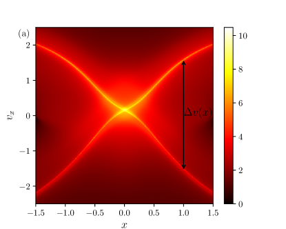
Figure 1: (a) Two-dimensional LD plot in the $xv_{x}$-plane. The function $\Delta v(x)$ is given by the difference in $v_{x}$ between the extreme values for the forward and backward time component of the LD. (b) Plot of the function $\Delta v(x)$ for the figure in (a). The dotted line indicates the value zero of the function.

One can use this approach to construct an algorithm to find the intersection of the closure of the stable and unstable manifold —i.e. the NHIM— as follows. First, at a given reaction coordinate $x$ and bath coordinates, one can perform an optimization in the reaction velocity $v_{x}$ extremizing the LD so as to obtain the associated positions of stable and unstable manifolds [see Fig. 1(a)]. From this, one computes their difference $\Delta v(x)$ in $v_{x}$-space as a function of the reaction coordinate $x$. A one-dimensional root search for $\Delta v(x_{0})=0$ [see Fig. 1(b)] yields the position $x_{0}$, where the stable and unstable manifold intersect, i.e., a point on the NHIM. This can be repeated for a set of bath coordinates and time to obtain the time-dependent NHIM up to the desired resolution.

Although one can readily identify the intersection of the manifolds in Fig. 1(a), the construction of a high accuracy image requires the computation of tens of thousands of trajectories and is only useful for demonstration purposes or to determine a rough estimate for the location of the NHIM. Meanwhile, the computation of a single value of $\Delta v(x)$ —i.e., a search of the manifolds for a fixed reaction coordinate— requires the computation of several LDs because extremal optimizations are in general iterative processes. This is especially taxing as one considers the fact that root finding methods, in and of themselves, are also iterative and require multiple values of $\Delta v(x)$ to provide accurate results. Doing so, provides a multiplicative factor to the required amount of computations. For multidimensional systems, these nested iterations have to be performed several times over large sets of bath coordinates, and this may easily result in the integration of several millions of trajectories.

II.2 Binary contraction method

In this section, we provide an alternative method that does not explicitly search for the stable and unstable manifolds, and thereby avoids the nested iterations of the LD approach. To accomplish this, we assume that the saddle region is an appropriate interval in the reaction coordinate $[x_{1},x_{2}]$ that covers the relevant dynamics of the time-dependent saddle. It can be found by sampling LDs in the region of interest, and has the structure shown in Fig. 1(a). In doing so, we are able to discriminate between four types of trajectories tied to one of four regions in phase space as shown in Fig. 2(a). Trajectories in regions (II) and (IV) are characterized as reactive, going from reactants to products and vice versa, respectively. Trajectories in regions (I) and (III) are non-reactive, remaining as products to products and reactants to reactants, respectively. Thus, every trajectory can be assigned to one of the four regions by integrating it forward and backward in time. While trajectories near the stable manifolds can spend a long time in the vicinity of the NHIM, they will eventually leave the barrier region when they are integrated sufficiently long. For orbits extremely close to the stable manifolds, the classification to the regions (I)-(IV) may nevertheless depend on rounding errors or numerical errors of the integrator, which means that the stable and unstable manifolds and thus the crossing point on the NHIM can only be determined with finite numerical accuracy. For the benchmark example of this work, the accuracy of the integrator was sufficient for the determination of the four regions as illustrated in Sec. III.1.

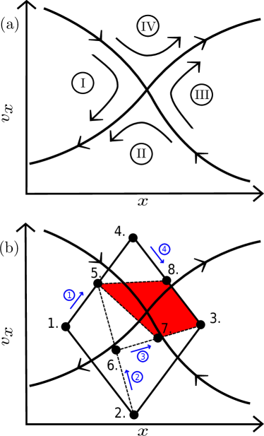
Figure 2: (a) View of the phase space in reaction coordinate and velocity. Stable and unstable manifold intersect and divide the plane in four regions marked by (I)–(IV). The dynamics in a region is dictated by the dynamics on the manifolds that form the region’s boundary. The arrows indicate the general path of trajectories in a positive time direction. (b) The intersection of the manifolds is found by contracting a quadrangle with a binary search algorithm applied to all four edges consecutively. The highlighted quadrangle is the result of contracting all edges of the quadrangle with the vertices 1, 2, 3, and 4 once in a counter-clockwise manner. The arrows with encircled numbers indicate the order and direction how vertices are replaced. The procedure can be iterated to obtain the intersection point with the desired accuracy.

Our binary contraction method is based on the observation that in the immediate vicinity of the hyperbolic point, the reactive and non-reactive regions are arbitrarily close to each other but still separated by stable and unstable manifolds. This is illustrated in Fig. 2(a). The manifolds associated with the NHIM determine the particle dynamics in the saddle region due to the asymptotic behavior of the related trajectories. More precisely, these regions determine which directions a particle enters and leaves the saddle region.

Similar to the LD method, we integrate the trajectories forward and backward in time. However, here the propagation of the trajectories does not occur for a fixed amount of time, rather each of the integrations in forward and backward time is stopped when the particle leaves the saddle region. This allows us to determine which of the four regions corresponds to the given initial phase space point. Using this information, we can construct a quadrangle in the $xv_{x}$-plane, with each vertex in one of the four regions. The algorithm is then divided into five steps [see Fig. 2(b)]:

1. Construct a quadrangle with each of its vertices in one of the four regions (I)–(IV).

2. Determine the midpoint between two adjacent vertices of the quadrangle.

3. Determine which region the midpoint corresponds to by integrating the dynamics in forward and backward time.

4. Use the new vertex to replace the vertex in the same region. (If the region identified for the midpoint is not identical to either of the original points, perform an error correction as described in Sec. II.2.2.)

5. Repeat steps 2–4 for all edges, e.g., in a counter-clockwise manner as in Fig. 2, until the longest edge of the quadrangle is below a desired error tolerance.

As implemented in our scheme, we walk through all the edges counterclockwise and successively in step 5. Alternative walks through the edges could provide faster or slower convergence, and the optimization of this scheme would be of possible interest to future work.

In Fig. 2(b), we illustrate these steps for the initial quadrangle with vertices $\{1,2,3,4\}$. First, our algorithm contracts vertices 1 and 4, leading to the new quadrangle $\{5,2,3,4\}$. It is then applied to vertices 5 and 2 to create $\{5,6,3,4\}$. In the next step, the new vertex 6 (and not one of the old vertex points as in the two previous steps) is replaced with vertex 7 resulting in $\{5,7,3,4\}$. After step 4, the highlighted quadrangle $\{5,7,3,8\}$ is created. Since this process is similar to a binary search algorithm, we call this method binary contraction.

Repeating this for all lines on the quadrangle ensures the reduction of mutual phase space distances between the vertices. Since reducing these distances in the $xv_{x}$-plane to an arbitrarily small size is only possible in the immediate vicinity of the hyperbolic point, we know that the quadrangle converges towards it. By computing the geometric center of the quadrangle in that plane, we have found the position of the hyperbolic point with an accuracy proportional to the size of the final quadrangle. By applying this method on a $xv_{x}$-plane of the reaction coordinates in a higher dimensional system, one can construct the NHIM $(x^{\mathrm{NHIM}}(\mathbf{y},\mathbf{v}_{y},t_{0}),v_{x}^{\mathrm{NHIM}}(\mathbf{y},\mathbf{v_{y}},t_{0}))$ for any suitable set of bath coordinates $(\mathbf{y},\mathbf{v_{y}})$ and initial time $t_{0}$. As the contraction still takes place on a two-dimensional plane, the efficiency of the method is not impacted by additional dimensions in phase space.

An efficient initialization of the quadrangle in step 1, as well as the error correction in step 4 will now be discussed in detail in Secs. II.2.1 and II.2.2, respectively.

II.2.1 Exception handling in initialization

An important prerequisite of the binary contraction method is the identification of good initial conditions for the iteration. To construct a valid quadrangle, we rely on the observation that the shape of the cross which divides the regions in the $xv_{x}$-plane is robust in the vicinity of the hyperbolic fixed point. The construction of the NHIM can be visualized readily with the help of an LD plot such as that shown in Fig. 1(a). One first constructs a quadrangle by guessing a phase space coordinate $(x_{0},v_{x_{0}})$ in the vicinity of the NHIM. Then one constructs the vertices with constant shifts in the $xv_{x}$-plane $\Delta x$ and $\Delta v_{x}$, such that $(x_{0}\pm\Delta x,v_{x_{0}})$ and $(x_{0},v_{x_{0}}\pm\Delta v_{x})$ form the vertices of the quadrangle.

For the initial set of selected vertices, we integrate the trajectories and compare their types to see if the construction of the required quadrangle was successful in the sense that there is a vertex in each of the 4 regions. If this is true, the iteration will start at this point. However some constructions may fail because they rely on both the accuracy of the guess and the size of the shifts. To mitigate this issue, one may increase shift sizes and try again. In addition, one can implement a bookkeeping method to combine valid vertices constructed from different shift sizes. Optimally, using a light-weight extrapolation method to determine an accurate guess from previous results would allow for a quick construction. This is especially efficient if we construct the NHIM in higher dimensions from a few already known points. In practice, a combination of both extrapolation and managed variation of shift sizes have proven to be highly effective for constructing the initial quadrangle.

One could also try to use an LD-based approach to determine points on the stable and unstable manifolds from which one can interpolate a valid quadrangle. However, because of the efficiency of the iteration in the binary contraction method, it would be ill-advised to use an initialization method that is computationally taxing in comparison, as the latter could dominate the runtime and overall cost of the computation.

II.2.2 Increasing convergence for edge cases

Depending on the choice of the underlying EOM and plane, one may run into situations where the borders of the regions form a heavily distorted cross. In situations like these, it is possible that the quadrangle contracts into an area where the intersection is not present, see Fig. 3. For an iteration that is completely inclusive —that is, one that contracts the quadrangle into a subset of itself— this may lead to convergence problems. This issue arises when the midpoint of a line is not contained in either of the regions of the original vertices, as this is the only situation where the quadrangle does not contract further.

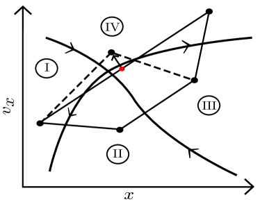
Figure 3: Edge case where a convergence failure may occur. The connecting line between vertices in regions (I) and (IV) crosses into other regions. The highlighted midpoint is detected to be in region (III) instead of (I) or (IV), and a new vertex is searched in the direction orthogonal to the connecting line. The dotted lines highlight the new quadrangle after a successful correction.

In that case, we allow the quadrangle to expand outward in the direction where the failure was discovered. The expansion is controlled such that the possible contraction of the iteration dominates.

Using this procedure, the quadrangle not only contracts around the intersection of the region, but also tumbles along the stable and unstable manifolds to actively center itself around the intersection. Although this procedure adds computational complexity to the iteration, we have observed that, on average, there is no noticeable increase in the computational time required. On the contrary, it even accelerates the computation for situations where convergence might not have been reached otherwise because it opens the quadrangle to more equally wrap around the targeted fixed point.

III Results

III.1 Tracing the motion of the NHIM for fixed bath coordinates

In this section, we will compare the performance of the LD-based method with nested iterations to the binary contraction method by computing several points on the NHIM and comparing the average number of necessary trajectories to compute a single point as a function of the algorithm’s tolerance. This is accomplished by applying both methods to a three-dimensional model system with a time-dependently moving rank-1 saddle. To this end, we use a three-dimensional extension of the two-dimensional time-dependent potential introduced in Ref. Feldmaier et al. (2017)

$$V(x,y,z,t) =E_{b}\exp{\left(-a{\left[x-\hat{x}\sin{(\omega_{x}t)}\right]}^{2}\right)}$$

$$+\frac{\omega_{y}^{2}}{2}{\left(y-\frac{2}{\pi}\arctan{(2x)}\right)}^{2}$$

$$+\frac{\omega_{z}^{2}}{2}{\left(z-\frac{2}{\pi}\arctan{(2x)}\right)}^{2}\ ,$$ (2)

and we use parameters in simulation units $E_{b}=2$, $a=1$, $\hat{x}=0.4$, $\omega_{x}=\pi$, $\omega_{y}=2$, and $\omega_{z}=1$. With these parameters, the potential has a periodicity of $T=2$. The algorithms are set to find a point on the NHIM for fixed bath coordinates $y=z=v_{y}=0$ and $v_{z}=0.5$, for 200 equidistant, initial time coordinates during one oscillation period, thereby tracing the NHIM’s time-dependent motion. Note that this tracing of the NHIM is not, in general, a trajectory of the system, since the results of the algorithms are not propagated by the dynamics of the system to find further points on the NHIM. Each point is computed separately. This allows us to control the accuracy of the data, as well as the specific bath coordinate for which the point is computed.

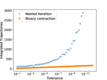
Figure 4: Number of integrated trajectories per hyperbolic fixed point found as function of the error tolerance of the algorithms. The difference in the scaling behavior is evident.

The results in Fig. 4 show that the binary contraction method requires far fewer trajectories to reach a given tolerance. Especially for very low tolerances, i.e., for high accuracy, it is highly superior in terms of performance. The difference in scaling is also quite evident, as the contraction exhibits an exponential convergence to the hyperbolic fixed point, while the performance of the nested iterations is clearly worse, even for large values of the tolerance. The fast convergence of the binary contraction method is evident from the fact that it divides the lengths of the quadrangle’s sides by roughly two for every successful iteration, therefore contracting the quadrangle exponentially fast.

Figure 5: The binary contraction in action for the model system with the time-dependent potential given in Eq. (2). One iteration corresponds to one counter-clockwise revolution around the quadrangle, contracting each side once, starting from the vertex line $\{1,2\}$ of the quadrangle $\{1,2,3,4\}$. In the next iteration the quadrangle $\{2,7,4,8\}$ is obtained. The LD values are shown through shading in the background, where one can clearly discern a cross which corresponds to the stable and unstable manifolds in the darkest shade. The quadrangles rapidly contract towards their intersection.

This is further illustrated in Fig. 5, where we apply the method to the model system with the time-dependent potential (2) for a specific choice of the bath coordinates and time. [Note that in this figure we use a different set of bath coordinates and time compared to Fig. 1(a).] The quadrangles of the first and second iteration are marked by numbers 1–8, and the dashed lines complete intermediate quadrangles. The quadrangles converge rapidly towards the intersection of the stable and unstable manifolds as marked by the largest values of the LD shown in the darkest shade of gray.

III.2 Propagation of trajectories initially in close vicinity to the NHIM

Using our method to efficiently compute high-accuracy points on the NHIM for any suitable bath coordinate and time, we investigate how trajectories deviate from the NHIM when they are started in its close vicinity. In this section, we present the results of an investigation for the model system defined in Eq. (2) as it is sufficient to illustrate the behavior even for systems with higher dimensionality as long as our earlier stated assumptions are satisfied.

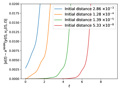
Figure 6: The $x$-coordinate distance of trajectories from the NHIM over time. The trajectories were propagated from the close vicinity of the NHIM with the initial position at increasing distances from the NHIM as listed in the legend and seen in the curves from left to right. Trajectories starting closer to the NHIM stay in its vicinity for a longer amount of time before deviating from it.

The binary contraction was performed to find the reaction coordinate $(x^{\mathrm{NHIM}},v_{x}^{\mathrm{NHIM}})$ of the NHIM for a given bath coordinate. The results of the contraction, performed for several different accuracies, are used as initial conditions for trajectories starting very close to the NHIM.

The properties of the resulting trajectories are shown in Fig. 6. Trajectories initially in close vicinity to the NHIM deviate exponentially from it, as expected. Those trajectories that started closer to the NHIM stay in its vicinity for longer time. When trajectories were initiated on the numerically computed NHIM, the situation was rather different in that they would also eventually deviate from the NHIM. In order to limit this deviation, the accuracy of the calculation had to be increased by continuing the iterative process of the contraction until the longest distance between adjacent vertices of the quadrangle was below $10^{-12}$. It is important to note that this accuracy only applies to the discrete dynamics of the numerically integrated system. The analytical accuracy of the trajectories is bound by the accuracy of the integration method used, as well as the size of the discrete time step. Nevertheless, for the discrete dynamics, this degree of accuracy can be achieved as long as sufficient numerical stability is provided. Consequently, the binary contraction method can indeed be used to obtain stable and accurate estimates of the NHIM up to the desired numerical accuracy.

IV Discussion

This work has been restricted to rank-1 saddles primarily because the construction of the time-dependent transition state trajectory remains a challenge even for this case. Much of the early work Bartsch et al. (2005a, b, 2006) on the transition state trajectory utilizing perturbation theory presumes such rank-1 saddles but is restricted by its radius of convergence. The more recent use of the LD was meant to get around this problem but it can be challenging when there is higher dimensionality Mendoza and Mancho (2010); Mancho et al. (2013); Craven and Hernandez (2015, 2016); Junginger et al. (2016); Junginger and Hernandez (2016a); Feldmaier et al. (2017). Below, we discuss the extent to which the binary contraction method addresses this challenge, and the implications on activated reactions with more general features.

The simple geometric structure drawn in, for example, Fig. 2 may appear to be a challenge to the binary contraction method for rank-1 barriers with multidimensional orthogonal coordinates. However, regardless of dimensionality the method contracts onto a quadrangle whose vertices reside on a two-dimensional plane via the midpoints between the vertices. The number of trajectories necessary to contract the quadrangle to the desired size does not increase with the dimensionality of the problem. However, the complexity of the equations of motion that may increase in higher dimensional systems will increase the computational cost of computing these trajectories. Additionally, one needs to keep in mind that even though the complexity of the contraction for a single point on the NHIM scales modestly with the dimensionality of the equations of motion, the number of points needed to characterize the NHIM for a given system may scale exponentially with its dimensionality, depending on how one chooses to construct the DS.

Although we have been successful in applying the binary contraction method to a system with a rank-1 saddle potential, we have yet to see how well it can be applied to systems with higher ranked saddle potentials, such as the systems investigated in Refs. 39; 40; 41, where the classification of trajectories is not as straightforward as for rank-1 saddle potentials because the characterization of the dynamics does not necessarily contract to the requisite quadrangle. Thus it remains to be seen if this approach can be extended to higher-rank saddles.

Another challenge to this and related approaches lies in its possible application to roaming pathways for which no clear saddle exists Townsend et al. (2004); Ulusoy et al. (2013); Maugière et al. (2014); Bowman and Suits (2011); Bowman (2014). However, if a NHIM exists for such a reaction, then that NHIM would by definition not be associated to a rank-1 saddle potential. This makes the identification of trajectories for the binary contraction even more of a challenge because the requisite quadrangle does not exist. Thus the future use of a binary contraction method to address roaming reactions would require a classification scheme to identify which trajectories —on a contracted two-dimensional surface— are reactive or not.

Finally, an additional concern for this and other related approaches addressing chemical reactions using transition state theory is whether quantum effects provide a significant correction Miller (1974); Garrett et al. (1982). Indeed, one of the constructions of semiclassical transition state theory has relied on the construction of the good-action variables that underlie the NIHM Miller (1977); Miller et al. (1990); Hernandez and Miller (1993); Hernandez (1994); Nguyen et al. (2011); Barker et al. (2012). Thus, one possible new direction beyond this work would involve the use of the binary contraction method to construct not use the NIHM but also an underlying coordinate space that represents the nonseparable but integrable coordinates needed to construct a semiclassical rate formula. However, this would only be necessary if the chosen system exhibits significant quantum effects. The present work is restricted to fully classical treatments of driven chemical reactions. Such dynamics arises frequently, particularly when heavy molecular motions occur in solution.

V Conclusion

We have introduced an exponentially converging algorithm that finds hyperbolic fixed points, i.e. the NHIM for non-autonomous systems with rank-1 saddles. The binary contraction method achieves the high efficiency by avoiding the explicit search for stable and unstable manifolds in nested iterations with LDs. The method relies on the identification of the saddle region, as well as the ability to describe the system in coordinates where the stable and unstable manifold intersect within two-dimensional planes in phase space.

By independently performing the algorithm on several two-dimensional planes one can map the NHIM via the bath coordinates of the system. We have discussed ideas to make this method reliable for difficult phase space structures, and methods for efficient initialization even in higher dimensions.

We have confirmed the relative stability of the NHIM computed numerically from the binary contraction method. Specifically, trajectories initiated on the time-dependent NHIM remain in its vicinity over time subject to the accuracy of the initial computation of the NHIM. The binary contraction method presented here is a useful advance to the existing set of methods for the comprehensive handling of driven chemical reactions. Using TST, fluxes and rates in such systems can be obtained by propagating a large ensemble of trajectories and determining the time when each trajectory crosses a time-dependent DS Feldmaier et al. (2017). The binary contraction method provides, in a first step, a large set of points on the NHIM, which can then be used, in a second step, to construct a time-dependent and locally recrossing-free DS by interpolating the discrete points on the NHIM. As with the other approaches —listed in the discussion in Sec. IV,— it remains challenging to address high dimensionality in the degrees of freedom orthogonal to the reaction coordinate. This could perhaps be resolved using machine learning methods, such as neural networks, as demonstrated in Ref. 34.

References

- Pitzer et al. (1962) K. S. Pitzer, F. T. Smith, and H. Eyring, The Transition State, Special Publ. (Chemical Society, London, 1962) p. 53.
- Pechukas (1981) P. Pechukas, Annu. Rev. Phys. Chem. 32, 159 (1981).
- Garrett and Truhlar (1979) B. C. Garrett and D. G. Truhlar, J. Phys. Chem. 83, 1052 (1979).
- Truhlar et al. (1985) D. G. Truhlar, A. D. Issacson, and B. C. Garrett, “Theory of chemical reaction dynamics,” (CRC Press, Boca Raton, FL, 1985) pp. 65–137.
- Natanson et al. (1991) G. A. Natanson, B. C. Garrett, T. N. Truong, T. Joseph, and D. G. Truhlar, J. Chem. Phys. 94, 7875 (1991).
- Truhlar et al. (1996) D. G. Truhlar, B. C. Garrett, and S. J. Klippenstein, J. Phys. Chem. 100, 12771 (1996).
- Truhlar and Garrett (2000) D. G. Truhlar and B. C. Garrett, J. Phys. Chem. B 104, 1069 (2000).
- Komatsuzaki and Berry (2001) T. Komatsuzaki and R. S. Berry, Proc. Natl. Acad. Sci. U.S.A. 98, 7666 (2001).
- Waalkens et al. (2008) H. Waalkens, R. Schubert, and S. Wiggins, Nonlinearity 21, R1 (2008).
- Bartsch et al. (2008) T. Bartsch, J. M. Moix, R. Hernandez, S. Kawai, and T. Uzer, Adv. Chem. Phys. 140, 191 (2008).
- Kawai and Komatsuzaki (2010) S. Kawai and T. Komatsuzaki, Phys. Rev. Lett. 105, 048304 (2010).
- Hernandez et al. (2010) R. Hernandez, T. Bartsch, and T. Uzer, Chem. Phys. 370, 270 (2010).
- Sharia and Henkelman (2016) O. Sharia and G. Henkelman, New J. Phys. 18, 013023 (2016).
- Lichtenberg and Liebermann (1982) A. J. Lichtenberg and M. A. Liebermann, Regular and Stochastic Motion (Springer, New York, 1982).
- Hernandez et al. (1993) R. Hernandez, W. H. Miller, C. B. Moore, and W. F. Polik, J. Chem. Phys. 99, 950 (1993).
- Ott (2002) E. Ott, Chaos in dynamical systems, second edition ed. (Cambridge University Press, Cambridge, 2002).
- Wiggins (2013) S. Wiggins, Normally hyperbolic invariant manifolds in dynamical systems, Vol. 105 (Springer Science & Business Media, 2013).
- Pollak and Pechukas (1978) E. Pollak and P. Pechukas, J. Chem. Phys. 69, 1218 (1978).
- Pechukas and Pollak (1979) P. Pechukas and E. Pollak, J. Chem. Phys. 71, 2062 (1979).
- Hernandez and Miller (1993) R. Hernandez and W. H. Miller, Chem. Phys. Lett. 214, 129 (1993).
- Hernandez (1994) R. Hernandez, J. Chem. Phys. 101, 9534 (1994).
- Uzer et al. (2002) T. Uzer, C. Jaffé, J. Palacián, P. Yanguas, and S. Wiggins, Nonlinearity 15, 957 (2002).
- Teramoto et al. (2011) H. Teramoto, M. Toda, and T. Komatsuzaki, Phys. Rev. Lett. 106, 054101 (2011).
- Li et al. (2006) C.-B. Li, A. Shoujiguchi, M. Toda, and T. Komatsuzaki, Phys. Rev. Lett. 97, 028302 (2006).
- Waalkens and Wiggins (2004) H. Waalkens and S. Wiggins, J. Phys. A 37, L435 (2004).
- Çiftçi and Waalkens (2013) U. Çiftçi and H. Waalkens, Phys. Rev. Lett. 110, 233201 (2013).
- Mendoza and Mancho (2010) C. Mendoza and A. M. Mancho, Phys. Rev. Lett. 105, 038501 (2010).
- Mancho et al. (2013) A. M. Mancho, S. Wiggins, J. Curbelo, and C. Mendoza, Commun. Nonlinear Sci. Numer. Simul. 18, 3530 (2013).
- Craven and Hernandez (2015) G. T. Craven and R. Hernandez, Phys. Rev. Lett. 115, 148301 (2015).
- Craven and Hernandez (2016) G. T. Craven and R. Hernandez, Phys. Chem. Chem. Phys. 18, 4008 (2016).
- Junginger et al. (2016) A. Junginger, G. T. Craven, T. Bartsch, F. Revuelta, F. Borondo, R. M. Benito, and R. Hernandez, Phys. Chem. Chem. Phys. 18, 30270 (2016).
- Junginger and Hernandez (2016a) A. Junginger and R. Hernandez, Phys. Chem. Chem. Phys. 18, 30282 (2016a).
- Feldmaier et al. (2017) M. Feldmaier, A. Junginger, J. Main, G. Wunner, and R. Hernandez, Chem. Phys. Lett. 687, 194 (2017).
- Schraft et al. (2018) P. Schraft, A. Junginger, M. Feldmaier, R. Bardakcioglu, J. Main, G. Wunner, and R. Hernandez, Phys. Rev. E 97, 042309 (2018).
- Junginger and Hernandez (2016b) A. Junginger and R. Hernandez, J. Phys. Chem. B 120, 1720 (2016b).
- Bartsch et al. (2005a) T. Bartsch, R. Hernandez, and T. Uzer, Phys. Rev. Lett. 95, 058301 (2005a).
- Bartsch et al. (2005b) T. Bartsch, T. Uzer, and R. Hernandez, J. Chem. Phys. 123, 204102 (2005b).
- Bartsch et al. (2006) T. Bartsch, T. Uzer, J. M. Moix, and R. Hernandez, J. Chem. Phys. 124, 244310 (2006).
- Haller et al. (2010) G. Haller, T. Uzer, J. Palacián, P. Yanguas, and C. Jaffé, Communications in Nonlinear Science and Numerical Simulation 15, 48 (2010).
- Haller et al. (2011) G. Haller, T. Uzer, J. Palacián, P. Yanguas, and C. Jaffé, Nonlinearity 24, 527 (2011).
- Nagahata et al. (2013) Y. Nagahata, H. Teramoto, C.-B. Li, S. Kawai, and T. Komatsuzaki, Phys. Rev. E 88, 042923 (2013).
- Townsend et al. (2004) D. Townsend, S. A. Lahankar, S. K. Lee, S. D. Chambreau, A. G. Suits, X. Zhang, J. L. Rheinecker, L. B. Harding, and J. M. Bowman, Science 306, 1158 (2004).
- Ulusoy et al. (2013) I. S. Ulusoy, J. F. Stanton, and R. Hernandez, J. Phys. Chem. A 117, 10567 (2013).
- Maugière et al. (2014) F. A. L. Maugière, P. Collins, G. Ezra, S. C. Farantos, and S. Wiggins, Chem. Phys. Lett. 592, 282 (2014).
- Bowman and Suits (2011) J. M. Bowman and A. G. Suits, Phys. Today 64, 33 (2011).
- Bowman (2014) J. M. Bowman, Mol. Phys. 112, 2516 (2014).
- Miller (1974) W. H. Miller, J. Chem. Phys. 61, 1823 (1974).
- Garrett et al. (1982) B. C. Garrett, A. D. Isaacson, R. T. Skodje, and D. G. Truhlar, J. Phys. Chem. 86, 2252 (1982).
- Miller (1977) W. H. Miller, Faraday Discuss. Chem. Soc. 62, 40 (1977).
- Miller et al. (1990) W. H. Miller, R. Hernandez, N. C. Handy, D. Jayatilaka, and A. Willetts, Chem. Phys. Lett. 172, 62 (1990).
- Nguyen et al. (2011) T. L. Nguyen, J. F. Stanton, and J. R. Barker, J. Phys. Chem. A 115, 5118 (2011).
- Barker et al. (2012) J. R. Barker, T. L. Nguyen, and J. F. Stanton, J. Phys. Chem. A 116, 6408 (2012).