The FRIED grid of mass loss rates for externally irradiated protoplanetary discs

Abstract

We present an open access grid of 3930 calculations of externally evaporating protoplanetary discs. This spans a range of disc sizes (1–400 AU), disc masses, UV field strengths (10–10⁴ G₀) and stellar masses (0.05–1.9 M_⊙). The grid is publicly available for download, and offers a means of cheaply including external photoevaporation in disc evolutionary calculations. It can also be queried using an online tool for quick estimates of instantaneous mass loss rates (e.g for convenient evaluation of real observed systems). fried itself illustrates that for discs around stars $\leq 0.3$ M_⊙ external photoevaporation is effective down to small radii ($<50$ AU) down to UV fields at least as weak as 10 G₀. At the other end of the scale, in a $10^{4}$ G₀ environment photoevaporation is effective down to 1 AU even for stellar masses at least as high as 1.9 M_⊙. We also illustrate in which regimes CO survives in the photoevaporative outflow for significant mass loss rates; marking a system a good candidate to detect external photoevaporation in weak–intermediate UV environments through sub–Keplerian rotation. Finally we make illustrative mass loss rate estimates for discs in Taurus based on the Guilloteau et al. (2011) star–disc parameters, finding that around half are expected to have both significant mass loss and retain CO in the photoevaporative outflow.

1 introduction

Planets are now known to exist around most stars (at least in the relatively local Milky Way) and exhibit a diverse range of architectures (Winn & Fabrycky, 2015). One of the key drivers in modern astrophysics is to understand the reason for this diversity, as well as how our own Solar system fits in to the wider population. To do so we must understand how the circumstellar “protoplanetary” discs of material around young stars not only ubiquitously give rise to planet formation, but also do so in a way that leads to high diversity in the resulting planetary parameters. To this end, substantial advances in our observational and theoretical capabilities have been made in recent years. Multi-wavelength observations from instruments like SPHERE (e.g. Garufi et al., 2017), ALMA (e.g. ALMA Partnership et al., 2015; Cieza et al., 2017; Fedele et al., 2018) and the GPI (e.g. Rapson et al., 2015; Currie et al., 2015) are giving us the best observational insight yet into the inner workings of protoplanetary discs and planet formation (for reviews and discussion on future advances see Williams & Cieza, 2011; Andrews, 2015; Sicilia-Aguilar et al., 2016). Similarly, theoretical models are making rapid advances to capture the rich physics of planet-forming discs, which includes chemistry, magnetic fields, dust and gas dynamics and radiation transport (for reviews and discussion of current and future advances in modelling of protoplanetary discs see Haworth et al., 2016a; Morbidelli & Raymond, 2016).

However, the problem is complicated further in that protoplanetary discs are found around young stars (the discs are typically dispersed well before 10Myr, e.g. Ribas et al., 2015) and young stars are typically still in the clusters from which they formed. There are therefore environmental factors that need to be accounted for. These are: one-off gravitational encounters, a binary (or tertiary, etc.) companion, and irradiation of a disc by other stellar members of the young cluster.

There is growing evidence that gravitational encounters are generally of secondary importance to photoevaporation. For example Scally & Clarke (2001) demonstrated this when comparing dynamical and radiative distruption of discs in an Orion like environment. Furthermore, Winter et al. (2018a) and Winter et al. (2018b) demonstrate that dynamical interactions are, statistically speaking, always a secondary effect in sculpting a disc population compared to photoevaporation, even in much weaker UV environments. Interactions have to be very close in order to see a significant effect on the disc evolution (Winter et al., 2018a). Protoplanetary discs can more obviously be affected by a binary companion, potentially being significantly disrupted as in the case of RW Aurigae (Cabrit et al., 2006; Dai et al., 2015; Rodriguez et al., 2018) truncated (Goldreich & Tremaine, 1980) or warped (Papaloizou & Pringle, 1983; Facchini et al., 2018). There is also evidence that this affects the resulting planetary populations (e.g. Zucker & Mazeh, 2002; Desidera & Barbieri, 2007).

The external photoevaporation of protoplanetary discs has been a challenging effect to gauge observationally. For many years, only the proplyds – discs within close proximity of O stars – were obviously observed to be photoevaporating (e.g. McCaughrean & O’dell, 1996; O’Dell, 1998, 2001; Henney et al., 2002). These are typically irradiated by a UV field of order $10^{5}$ G₀. The effects of photoevaporation in the vicinity of O stars have also been studied recently by, for example, Ansdell et al. (2017), Eisner et al. (2018) using the spatial distribution of disc properties. Some direct measures of the mass loss rate from discs near O stars have been made, for example by Churchwell et al. (1987), Henney & O’Dell (1999) and Henney et al. (2002), finding mass loss rates of order $10^{-6}$ M_⊙ yr^-1.

In recent years there has been growing evidence of external photoevaporation in weaker radiation environments. Kim et al. (2016) found proplyds in a $\sim 3\times 10^{3}$ G₀ environment and Haworth et al. (2017) used numerical models to propose external photoevaporation as the reason for the large CO halo around IM Lup, which is only in a $\sim 4$ G₀ environment (Cleeves et al., 2016). Nevertheless, external photoevaporation in weak–intermediate radiation environments is generally unconstrained, in part because it has not yet been actively searched for since the signatures of external photoevaporation aren’t well known. As most stars are not in such a strong UV environment as the proplyds (Fatuzzo & Adams, 2008) understanding the evolution of discs in weaker environments is important.

Modelling the external photoevaporation of discs is difficult because the thermodynamic properties of the flow are set by photodissociation physics for the UV fields that the majority of star–discs are exposed to (in the limit of being very close to a strong EUV source, photoionisation dominates, see Figure 12 of Winter et al., 2018b). Computing the thermal structure of a photodissociation region (PDR) requires the solution of a chemical network that is also sensitive to the non-local distribution of matter. That is, the temperature at one point in the flow is sensitive to the rest of the flow structure because this sets the cooling by the escape of line photons and also the attenuation of the UV field by dust/molecular self-shielding in outward lying regions of the photoevaporative flow. For this reason, for a long time only semi-analytic models of the flow structure and hence mass loss rate could be produced (e.g. Hollenbach et al., 1994; Johnstone et al., 1998; Adams et al., 2004; Facchini et al., 2016). These are quick to compute but are only able to obtain solutions in certain subsets of parameter space. To date they also all only consider 1 M_⊙ stars.

Computing solutions for arbitrary parts of the parameter space requires full photochemical-dynamical models that iteratively solve the PDR chemistry/temperature with the dynamics. This is both difficult to implement and computationally expensive, but has now been achieved by Haworth et al. (2016b) using the torus-3dpdr code (discussed in section 3.1). Because these mass loss rates are difficult to compute, and expensive, having a large grid of publicly available pre-computed models would therefore open up consideration of external photoevaporation to the wider community.

The value of pre-computed mass loss rates from models such as the above is that they can either be used to estimate the instantaneous mass loss rate for real systems, or can be applied to viscous evolutionary models of discs (Clarke, 2007; Anderson et al., 2013; Kalyaan et al., 2015; Haworth et al., 2017, 2018; Winter et al., 2018b).

In this paper we present the results of a large grid of external photoevaporation models as described above, which we refer to as the fried (FUV Radiation Induced Evaporation of Discs) grid. This covers a wide parameter space of stellar mass, disc mass, disc radius and UV field. It is publicly available for direct download, but we also provide an online tool for making quick mass loss rate estimates. The rest of this paper is as follows. In section 3 we discuss how the fried grid is constructed, in section 4 we provide an overview of the resulting grid and the online resources. Finally in section 5 we apply the grid to an illustrative population of discs.

2 Preamble: easy access summary

Our aim is for the grid of models in this paper to be widely used, and for both theoretical and observational applications. Since the models themselves are rather technical we therefore begin with a more accessible summary of the grid.

We have calculated the mass loss rate of gas (the mass loss rate of dust is related to, but different from the gas mass loss rate, Facchini et al., 2016; Haworth et al., 2018) from protoplanetary discs that are stripped of material due to external irradiation by nearby stars. We have done this for a large variety of stellar/disc parameters as well as UV field strengths and tabulated this in the fried grid. Estimating this mass loss rate directly (without our grid) is both technically and computationally challenging, and so isn’t usually considered either observationally or in numerical models.

The grid itself is summarised in Figures 5-9, which each show the mass loss rate (colour scale) as a function of disc size ($y-$axis), disc mass ($x-$axis), and stellar mass in UV environments of $10$, $10^{2}$, $10^{3}$, $5\times 10^{3}$ and $10^{4}$ G₀ respectively. Each panel in these Figures represents a different stellar mass. Having these mass loss rate estimates over such a large parameter space allows estimates of the instantaneous mass loss rate to be made for real observed systems. That is, if you know the stellar mass, disc mass and disc radius you could estimate the mass loss rate as a function of the UV field (and similarly for other combinations of known/unknown parameters).

To use the grid, the most efficient and flexible way is to download it in its entirety. There is also an online tool for which you can provide the star–disc parameters and it will interpolate and return a mass loss rate (discussed in more detail in section 4.3).

At present fried includes only a single metallicity/PAH option, but can expand to accommodate this in future releases.

3 constructing the fried grid

Here we describe the construction of our grid of photoevaporation models in detail. We begin by discussing the details of any given individual calculation and then discuss the coverage of the grid in section 3.4.

3.1 Photoevaporation calculations

The disc photoevaporation calculations are computed using the torus-3dpdr extension (Bisbas et al., 2015) of the torus Monte Carlo radiation transport and hydrodynamics code (Harries, 2000; Haworth et al., 2015; Ali et al., 2018). The approach is very similar to that first detailed and benchmarked in Haworth et al. (2016b).

The models involve iteratively performing hydrodynamics steps over some time interval $\Delta t$ and PDR chemistry calculations. The thermal properties set by the PDR calculation then set the pressure distribution in the dynamical step. The calculations in this paper are 1D spherical, with the bulk of the mass loss assumed to be driven from the disc outer edge, where there is a large mass reservoir that is least gravitationally bound to the star (see Adams et al., 2004, for a discussion on this). Under such a scheme the mass loss rate is

$$\dot{M}_{w}=4\pi R^{2}\rho\dot{R}\mathcal{F}$$ (1)

where $\dot{R}$ is the flow velocity, with density $\rho$ at distance $R$, and $\mathcal{F}$ is the fraction of solid angle subtended by the disc outer edge $R_{d}$, which Adams et al. (2004) define as

$$\mathcal{F}=\frac{H_{d}}{\sqrt{H_{d}^{2}+R_{d}^{2}}}$$ (2)

The hydrodynamics itself is a grid based finite volume scheme with a point source gravitational potential set by the parent star. We generally use a van Leer (1979) flux limiter and a Courant–Friedrichs–Lewy parameter of 0.3.

The PDR calculation considers 33 species and 330 reactions, and was tailored to give temperatures accurate to within around 10 per cent of the UMIST 2012 chemical network database of 215 species and over 3000 reactions (McElroy et al., 2013). A summary of the species included and the initial abundances assumed is given in Table 1. Note that chemical equilibrium is assumed, so the initial abundances are unimportant other than to set the initial distribution of metals and computational time taken to reach equilibrium. In the models of Haworth et al. (2016b), which are similar to those here, we justified the assumption of equilibrium by showing that the thermal timescale was indeed faster than the flow timescale. Recently, time-dependent models tailored to the study the FUV internal photoevaporation of discs by the host star have been computed by Wang & Goodman (2017) and Nakatani et al. (2018).

The main cooling in these models is the escape of line photons of C I, C II, O I and CO (see the right hand panel in Figure 2 of Facchini et al., 2016). PAH heating is potentially the most important heating mechanism (left hand panel in Figure 2 of Facchini et al., 2016). The PAH abundance in the outer regions of discs is highly uncertain, with some evidence for depletion in the outer disc (e.g. Geers et al., 2006; Oliveira et al., 2010; Perez-Becker & Chiang, 2011). The PAH scheme used in torus-3dpdr follows Wolfire et al. (2003) and assumes a PAH–to–dust mass ratio for the ISM of $2.6\times 10^{-2}$. In prior studies of external disc photoevaporation Facchini et al. (2016) assumed this ISM like PAH abundance and Haworth et al. (2017), Haworth et al. (2018) conservatively assumed a negligible PAH abundance. Similarly Gorti et al. (2015) use a low PAH abundance of one hundredth the ISM value. Here we choose an intermediate option. Given the abundance uncertainty and possible depletion at large radii of PAHs in discs, for this initial grid we use a PAH abundance of 10 per cent the canonical ISM value, i.e. a PAH-to-dust mass ratio of $2.6\times 10^{-3}$.

The grid could be expanded in future to account for variations in PAH abundance and/or metallicity. Following Facchini et al. (2016) at this stage for simplicitys we always assume a mean particle mass of 1.3 in the hydrodynamics.

Table 1: The upper section is a summary of the species included and initial gas abundances for the reduced network used in this paper. The sum of hydrogen atoms in atomic and molecular hydrogen is unity. The other abundances are with respect to the sum of hydrogen. The lower sections summarise the other microphysical parameters.

Gas
Species	Initial abundance	Species	Initial abundance
H	$4\times 10^{-1}$	H2	$3\times 10^{-1}$
He	$8.5\times 10^{-2}$	C+	$2.692\times 10^{-4}$
O	$4.898\times 10^{-4}$	Mg+	$3.981\times 10^{-5}$
H+	0	H2+	0
H3+	0	He+	0
O+	0	O2	0
O2+	0	OH+	0
C	0	CO	0
CO+	0	OH	0
HCO+	0	Mg	0
H2O	0	H2O+	0
H3O	0	CH	0
CH+	0	CH2	0
CH2+	0	CH3	0
CH3+	0	CH4	0
CH4+	0	CH5+	0
e-	0
Dust
$\sigma_{\textrm{FUV}}$	$2.7\times 10^{-23}$ cm2	Cross section in wind
$\delta$	$3\times 10^{-4}$	Dust-to-gas mass ratio in wind
$f_{\textrm{PAH}}$	0.1	PAH abundance relative to ISM
$\delta_{\textrm{PAH}}$	$2.6\times 10^{-3}$	PAH-to-dust mass ratio
Other
$\zeta$	$5\times 10^{-17}$ s-1	Cosmic ray ionisation rate

3.2 Disc construction

Across our parameter space we are computing the mass loss rate in the photoevaporative wind $\dot{M_{w}}$ as a function of the stellar mass $M_{*}$, disc mass $M_{d}$, disc radius $R_{d}$ and incident UV field strength $G_{0}$. For each model we set up a disc structure, which acts as a boundary condition to the photoevaporative wind and is not allowed to dynamically evolve.

For the disc that sets the boundary condition to the flow we consider a truncated power law surface density profile

$$\Sigma(R)=\Sigma_{1\textrm{AU}}\left(\frac{R}{\textrm{AU}}\right)^{-1}$$ (3)

where

$$\Sigma_{1\textrm{AU}}=\frac{M_{d}}{2\pi R_{d}\,1\textrm{AU}}$$ (4)

Given that our calculations are 1D we require a volume density from a scale height

$$H=\frac{c_{s}}{\Omega}$$ (5)

and

$$\rho_{\textrm{mid}}=\frac{\Sigma(R)}{\sqrt{2\pi}H}.$$ (6)

Unless the disc is externally heated above the temperature set by the central star, the thermal structure in the disc is assumed to be of the form

$$T=T_{1\textrm{AU}}\left(\frac{R}{AU}\right)^{-1/2}$$ (7)

where $T_{1AU}$ is assumed to vary with stellar mass according to

$$T_{1\textrm{AU}}=100\left(\frac{M_{*}}{M_{\odot}}\right)^{1/4}\,\textrm{K}.$$ (8)

The above is imposed out to some disc outer radius $R_{d}$ (the values of which are summarised in section 3.4). The remainder of the computational domain (see section 3.3) freely evolves until it reaches a steady state. Note that the mass loss rate is only sensitive to the disc outer edge, so although we set the conditions there in terms of some global disc properties (e.g. equation 3, and referring to a “disc mass”) the interior parts of the disc could be different and still give the same mass loss rate if the outer disc were the same.

The disc itself can also be heated by the external UV field. We apply the maximum of temperatures given by equation 7 and that computed in the PDR calculation, both within in the disc (which modifies the scale height) and in the flow. External irradiation can hence lower the mid-plane density and increase the scale height of the disc, which in turn can affect the mass loss rate compared to a model where the disc itself is assumed to never be externally heated.

We also impose a limit on where the photodissociation region (PDR) microphysics is applicable. In 1D models high density, highly optically thick regions can lead to spurious heating in PDR codes as the escape probability of cooling photons tends to zero. Therefore, interior to the point in the flow with an extinction greater than 10 and a gas local number density exceeding $10^{8}$ cm^-3 we assume that the temperature of the flow is constant until heating from the star dominates. This is the approach used by Facchini et al. (2016) and Haworth et al. (2018).

3.3 Other calculation parameters

All models in the fried grid use an adaptive mesh, with higher refinement on the simulation domain when and where it is required. For the bulk of our calculations the grid size is 1000 AU with a maximum resolution of $0.49$ AU. For the models with $R_{d}=5$ AU and $1$ AU we use grid sizes of 668 and 334 AU and maximum resolution of 0.33 and 0.16 AU respectively.

A unique solution for a steady transonic flow corresponds to the case where the flow satisfies criticality conditions (simultaneous vanishing of terms in the combined momentum and continuity equations, e.g. Parker, 1965; Clarke & Alexander, 2016) at some point in the flow. Our numerical scheme will only converge on this solution if the critical point is contained within the grid. For a radial flow where temperature is a function of optical depth and local density, the criticality condition can be written (Facchini et al., 2016):

$$\frac{v^{2}\mu m_{\textrm{H}}}{k_{\textrm{B}}}-T-n\frac{\textrm{d}T}{\textrm{d}n}\geq 0.$$ (9)

We therefore retrospectively checked that this was the case, using neighbouring cells for the derivative, and re-ran calculations where necessary with a larger grid.

3.4 Scope of the FRIED grid

Our large grid consists of models that are systematically varied. We include stellar masses of 0.05, 0.1, 0.3, 0.5, 0.8, 1, 1.3, 1.6 1.9 M_⊙. For each of these stellar masses we model disc masses in a 400 AU disc that would have been $3.2\times 10^{-3}$, 0.1, 1.12, 3.16, 8.94 and 20 per cent the stellar mass. We then consider this disc surface density profile truncated at 1, 5, 10, 20, 30, 40, 50, 75, 100, 150, 200, 250, 300, 350, 400 AU. Finally, for each of these stellar/disc parameters, we consider incident UV fields of 10, $10^{2}$, $10^{3}$, $5\times 10^{3}$ and $10^{4}$ G₀. Note that in practice in a $10^{4}$ G₀ environment there will also be a strong EUV field, which is not included here. Overall this leads to a substantial grid of 4050 models, though we discard some of the very lowest mass disc models in the 0.05 and 0.1 M_⊙ star cases that appear numerically unstable, leaving us with 3930 models. In this first iteration of the fried grid we consider only a single metallicity and polycyclic aromatic hydrocarbon (PAH) abundance (detailed above in section 3.1), though in future we could extend the grid to explore this.

3.5 Illustrative calculation

Finally, before presenting the grid itself we illustrate the manner of a single of calculation in detail so the reader can better appreciate the material underlying the grid. Figure 1 shows a series of profiles for a 100 AU, 23.4 M${}_{\textsc{jup}}$ disc around a 1 M_⊙ star. The top left panel shows the steady state number density profile and mass loss rate profile, with the black vertical line denoting the disc outer edge. In this first panel results from 3 different times are included. There are small variations in the mass loss profile due to numerically induced velocity perturbations induced at the disc outer edge boundary condition, but the mass loss rate is otherwise very steady at $\log_{10}(\dot{M})\sim-6.155$. The upper right panel shows the gas and dust temperature profile. The second row, left panel shows the outward gas velocity and local sound speed profiles. In this case the jump to a supersonic flow coincides with the critical point in the flow, which is illustrated by the crossing of 0 in the lower left hand panel.

The second row, right hand panel of Figure 1 shows the azimuthal and Keplerian velocity. Deviation from Keplerian velocity is one possible way of detecting external photoevaporation as pointed out by Facchini et al. (2016) and Haworth et al. (2016b) and possibly identified in the case of IM Lup by Pinte et al. (2018). The third row left and right hand panels show the extinction and UV profiles and the lower right shows the abundance profile of a small fraction of the 33 species in the network. Note that although our initial abundances in Table 1 are atomic/ionic, once a steady state is achieved the disc (as well as the inner part of the flow itself) is molecular, and molecular line cooling plays an important role in setting the thermal balance there.

This makes up just one of the 3930 models of the fried grid which are all similarly complex.

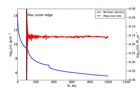
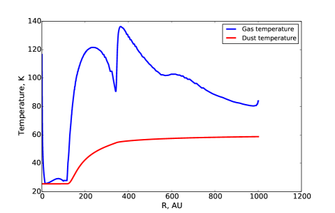
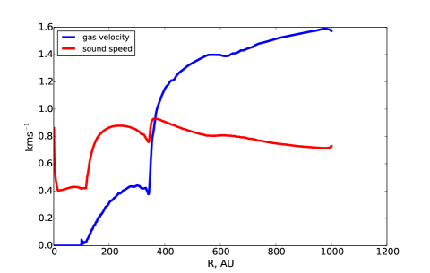
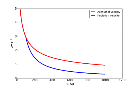
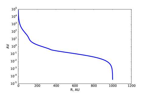
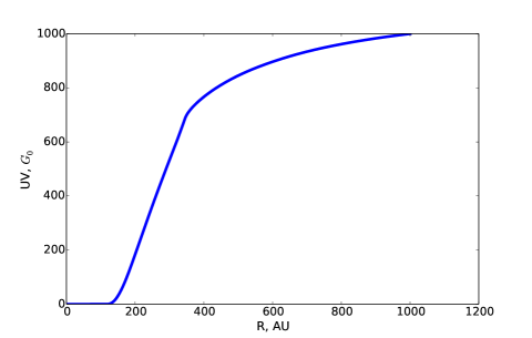
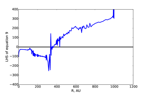
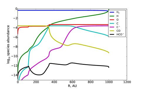
Figure 1: A selection of properties of a 100 AU, 23.4 M${}_{\textsc{jup}}$ disc around a 1 M_⊙ star being irradiated by a $10^{3}$ G₀ UV field. From left to right, top to bottom these are: the density and mass loss rate (in this panel both are plotted at 3 different times), gas and dust temperature, gas velocity/sound speed, azimuthal and Keplerian velocity, extinction and UV. The left hand lower panel shows the critical point: that at which the left hand side of equation 9 first crosses zero. The lower right hand panel shows the abundance profile of various species

4 The fried grid

4.1 Mass loss rates

The mass loss rates over the entire grid are summarised in Figures 5–9. Each figure consists of a series of panels plotting the mass loss rate as a function of the disc size and mass. The different panels in each figure correspond to different stellar masses, as indicated above each panel. We do not intend to describe each component of the grid in detail, but note the following highlights before considering some immediate consequences in section 5.

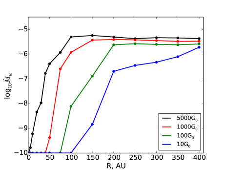
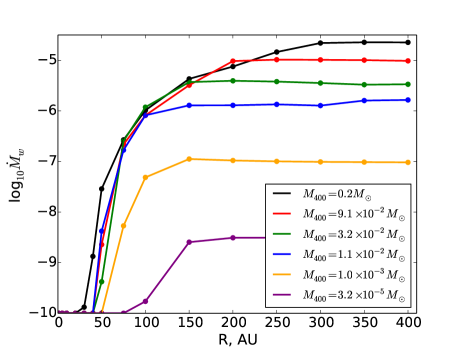
Figure 2: Illustrative mass loss rates as a function of disc outer radius. The left hand panel varies the UV field strength incident upon a $2.2\times 10^{-2}$ M_⊙, 100 AU disc. The right hand panel varies the disc mass out to 400 AU for a fixed UV field of 1000 G₀. All of the above are for a 1 M_⊙ star

1. An illustration of mass loss rates as a function of radius is given in Figure 2. The left hand panel holds the star–disc parameters constant, but varies the incident UV field strength. The right hand panel is for a $10^{3}$ G₀ field, but different disc masses. The disc size at which external evaporation is ineffective increases with decreasing UV field strength. For a fixed UV field strength the mass loss rate increases with the disc mass, but the radius at which external photoevaporation becomes ineffective is relatively constant. We struggle to find steady state mass loss rates below $10^{-10}$ M_⊙ yr^-1, so impose this as the floor value of the grid. This is lower than the internal mass loss rate due to EUV/X-rays (e.g. Owen et al., 2012).
   

2. For UV fields $<10^{4}$ G₀, as the stellar mass increases photoevaporation becomes ineffective out to larger and larger disc radii. For example in the 10 G₀ case, for a 1 M_⊙ star photoevaporation is ineffective for discs $<100$ AU in size (see the middle right panel of Figure 5), but in the 0.1 M_⊙ case photoevaporation is effective down to $\sim 10$ AU (top middle pane of Figure 5).
   

3. In the $10^{4}$ G₀ case (Figure 9) photoevaporation is effective at all radii for all stellar masses that we consider (up to 1.9 M_⊙). This is because the UV field is high enough that it can still heat the disc to a sufficient extent that a wind can be driven, even when it is very compact. This implies that an infrared excess due to small grains would disappear very quickly for discs in regions such as the Orion Nebular Cluster (ONC) especially given the additional effects of EUV heating (not included here) in this environment.
   

4. In the lowest stellar mass cases (0.05 and 0.1 M_⊙) the mass loss rate is relatively insensitive to the UV field strength for extended discs ($R_{d}>\sim 20$ AU). For example for a 100 AU, 0.15 M${}_{\textrm{jup}}$ disc around a 0.05 M_⊙ star the mass loss rate increases by only around 1 per cent from 10 to $10^{4}$ G₀. The temperature in the flow does steadily increase with UV field strength, resulting a more rarefied, but also faster flow. This lower density in the flow coupled with higher velocity as the UV field increases means that the mass loss rate stays approximately constant.
   

5. Discs around low mass stars ($\leq 0.3$ M_⊙) are evaporated down to small radii ($<50$ AU) much more effectively than higher mass stellar systems. This is because the disc is less gravitationally bound to a lower mass parent star.
   

4.2 Behaviour as $R_{\textrm{H}-\textrm{H}_{2}}\rightarrow R_{d}$

Despite the $10^{4}$ G₀ case giving significant mass loss down to the smallest disc outer radii (see Figure 9), it can exhibit slightly lower mass loss rates than in the $(5\times)10^{3}$ G₀ cases at larger disc outer radii. We explored this using some additional models for a 100 AU disc around a 1 M_⊙ star with incident UV fields from $2\times 10^{3}-1.5\times 10^{4}$ G₀.

The Facchini et al. (2016) critical point (equation 9) is usually in the molecular part of the wind, with the H–H₂ transition at some larger radius. Comparing these two locations, we find that the drop in mass loss rate at high UV is associated with the H–H₂ transition becoming coincident with the critical point. In Figure 3 we show the mass loss rate as a function of UV field strength for the additional exploratory models, with points colour coded by the ratio of the critical radius to that of the H–H₂ transition. This clearly illustrates that the mass loss rate drop at $\sim 7000$ G₀ is associated with the critical radius being coincident with the H–H₂ transition.

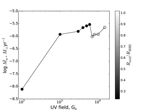
Figure 3: The mass loss rate as a function of UV field strength for the model that we explore in more detail to probe the regime where the H–H₂ transition influences the mass loss rate. The colour scale denotes the ratio of the critical radius to the radius of the H–H₂ transition. Their coincidence results in a drop in the mass loss rate.

We will present a physical description of the flow in this new regime in a subsequent paper, but note now that it shows some similarities to prior analytic work in which the hydrogen ionisation front sets the mass loss rate (e.g. Johnstone et al., 1998), only with added complications such as the fact that the change in sound speed across the H–H₂ transition is unknown.

4.3 Online resources

The raw mass loss rate grids are available for download both as online material accompanying this journal article and from the fried website. In addition to this, we have developed a web interface that allows users to quickly and easily estimate mass loss rates for arbitrary disc/UV field parameters. In its current form the user specifies a disc extent, disc mass and stellar mass. Values of the mass loss rate for a range of UV field strengths are then returned using a linear interpolation over the grid with the python scipy LinearNDInterpolator routine. We choose a linear interpolation because it is straightforward and robust, unlike higher order schemes which could possibly give rise to oscillations. Of course by downloading the entire grid a more sophisticated interpolation can be applied at the users own discretion and risk. The online tool does not permit queries to be made beyond the bounds of the grid parameter space. For special cases contact the authors to discuss either expanding the grid or running bespoke models for a given application.

The intention is that the online tool can be easily be used by theorists and observers alike to quickly gauge whether significant photoevaporation is occuring in a given scenario. An illustrative example of application of the fried grid to real systems is given in section 5.2.

5 Discussion

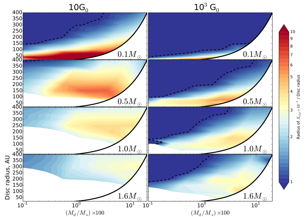
Figure 4: The ratio of the extent out to which CO is abundant to the extent of the Keplerian disc, as a function of disc size and the ratio of disc–to–stellar mass. The dashed contours denote the point at which CO is depleted at the disc outer edge. Models with mass loss rates less than $10^{-9}$ M_⊙ yr^-1 are not included and the region below the solid black line is not included in our parameter space. The left and right hand panels are for UV fields of 10 and $10^{3}$ G₀ respectively and the stellar mass 0.1, 0.5, 1 and 1.6 $M_{\odot}$ from top to bottom. If CO extends beyond the disc outer edge, then it is possible it could be used to detect the photoevaporative wind, for example through a sub-Keplerian rotation profile or a radially increasing temperature measured with CO line ratios. Note that since the grid extent is typically 1000 AU, some of the ratios presented here may be lower limits if the grid size is what limits the CO extent.

5.1 Constraints on detecting external photoevaporation using CO in weak–intermediate UV regimes

The PDR thermal physics in our models also contains information on the chemical structure of the flow which could provide clues as to the best scenarios in which to search for external photoevaporation in action. CO observations towards discs are common, but typically focus on rings and gaps in the main body of the disc, rather than the outer disc where external photoevaporation is expected to be strongest. Two possible signatures of external photoevaporation in CO are sub-Keplerian rotation in the outer disc (Facchini et al., 2016; Haworth et al., 2016b) and a radially increasing temperature profile. Sub-Keplerian rotation in the candidate evaporating disc IM Lup (Cleeves et al., 2016; Haworth et al., 2017) has been detected by Pinte et al. (2018). A radially increasing temperature profile could be probed using CO line ratios.

Given the above and current lack of other diagnostics, of specific interest are regions of the parameter space where a kinematic and thermal tracer such as CO is observable and the mass loss rate is non-negligible (and, ideally, the deviation from Keplerian rotation is spectrally resolvable). We therefore compute the ratio of the radius at which CO is reduced in abundance ($R_{\textrm{CO}}$) to the disc outer radius ($R_{\textrm{disc}}$). This transition happens quickly, so we mark the point at which the CO abundance drops to less than $10^{-5}$. Note that the role of different reactions as well as cosmic rays and photodissociation on setting the CO abundance are well known and the reader is directed to van Dishoeck & Black (1986) and van Dishoeck & Black (1988) for more information. Values of $R_{\textrm{CO}}/R_{\textrm{disc}}>1$ therefore have CO abundant in the photoevaporative wind. Of these models, we then only retain those in which the mass loss rate is greater than $10^{-9}$ M_⊙ yr^-1. This leaves us with a grid of models that summarise the best regimes in which it might be possible to probe a photoevaporative wind using CO.

Figure 4 summarises this dataset for a 0.1, 0.5, 1 and 1.6 M_⊙ stars in 10 and $10^{3}$ G₀ environments. In the low UV case if the stellar mass is low then CO is abundant in the flow and there is still significant mass loss down to small disc outer radii ($<50$ AU). However at higher stellar masses there is a lower limit on the radius of the disc at which the mass loss rate is actually significant. At higher UV field strengths in the low stellar mass scenario CO is depleted in the photoevaporative wind except for very compact discs. Conversely for higher stellar masses CO is abundant and has significant mass loss down to smaller disc outer radii than in the 10 G₀ case. Discs around $1-2$ M_⊙ stars in $\sim 10^{3}$ G₀ environments therefore seem to provide a good opportunity to identify external photoevaporation in action.

Another interesting point to note is that the typical factor 2 or more extent of CO relative to the Keplerian disc outer edge is large enough to account for the observed extent of the gas relative to dust in Lupus discs by Ansdell et al. (2018). Since only small grains are entrained in a photoevaporative wind (Facchini et al., 2016) and hence will not be detected in the millimetre continuum this raises the possibility that external photoevaporation might be a contributing factor in setting the observed relative gas–dust disc sizes. However this has the caveat that we cannot robustly constrain the surface brightness in CO from 1D models so cannot currently predict the observable CO extent, just that out to which it is abundant.

5.2 Illustrative instantaneous mass loss rate estimates for real systems: Taurus discs

The fried grid makes it trivial to estimate mass loss rates for real systems based on estimates of the stellar mass, disc mass, disc radius and incident UV field strength. In cases where not all of these are known, the grid can be used to assess ranges of plausible values.

Table 2: Illustrative mass loss rates for real systems for a range of UV field strengths. All star-disc parameters are from Guilloteau et al. (2011).

System	$M_{*}(M_{\odot})$	$M_{d}(10^{-3}\,M_{\odot})$	$R_{d}$ (AU)	$\dot{M}(M_{\odot}\,\textrm{yr}^{-1})$	CO in flow?	High/Medium/Low
				$10G_{0}$	(Figure 1)	Mass loss rate
BP Tau	0.78	5.4	57.	$10^{-10}$	–	L
CI Tau	0.76	37	201.	$4.6\times 10^{-7}$	Y	H
CQ Tau	1.7	6.3	188.0	$2.6\times 10^{-10}$	–	L
CY Tau	0.48	16.5	92.	$9.9\times 10^{-8}$	Y	H
DG Tau	0.7	36.0	198.	$5.2\times 10^{-7}$	Y	H
DL Tau	0.7	49.0	179.	$1.8\times 10^{-7}$	Y	H
DM Tau	0.47	31.1	274.	$2.8\times 10^{-6}$	Y	H
DQ Tau	0.55	12.1	439.	$3.6\times 10^{-7}$	–	H
GM Aur	1.37	27.0	578.	$8.9\times 10^{-7}$	–	H
Lk Ca 15	1.12	28.4	178.	$2.3\times 10^{-8}$	Y	H
MWC480	1.8	182.3	155.	?	–	?
MWC758	1.8	10.6	187.	$2.3\times 10^{-9}$	–	M
HL Tau	0.7	90.6	280.16	$3.7\times 10^{-6}$	Y	H
HH 30	0.25	8.1	123.	$7.5\times 10^{-7}$	Y	H
DG Tau B	3.0	67.9	303.	?	–	?
T Tau N	1.9	0.1	67.	$10^{-10}$	–	L
Haro6-13	0.55	0.6	90.	$4.9\times 10^{-10}$	–	L
Haro6-33	0.55	0.5	439.	$2.6\times 10^{-8}$	–	H

In Table 2 we calculate the mass loss rate for the dust disc extents and masses in Taurus inferred by Guilloteau et al. (2011). PDR modelling of Taurus requires an average UV field of around 10 G₀ according to Heiner & Vázquez-Semadeni (2013) to give consistent H i and CO observations, so we adopt this UV field strength for our illustrative assessment. For discs larger than 400 AU (the upper limit on our grid) we set the disc radius to 400 AU, which is, if anything, an underestimate of the mass loss rate (see Figure 1). We do not similarly limit the disc mass. These estimates are based on dust disc radii, so given the gas is generally found to be more extended (e.g. de Gregorio-Monsalvo et al., 2013; Facchini et al., 2017) and mass loss rates are higher for larger discs it is quite a conservative estimate.

In the sixth column of Table 2 we note whether each disc has CO in the flow from Figure 4. In the final column of Table 2 we denote any system in which the mass loss rate is above $10^{-8}$ M_⊙ yr^-1 a high mass loss rate (H), otherwise if the mass loss rate is above $10^{-9}$ M_⊙ yr^-1 we denote it “medium” (M), else the mass loss rate is low (L). In two cases, MWC 480 and DG Tau B, the disc mass is extremely high, so the fried grid is unable to compute a reliable mass loss rate estimate.

At least half of the discs in our illustrative application have significant mass loss rates ($>10^{-8}$ M_⊙ yr^-1) in a 10 G₀ environment. Of these discs with high mass loss rates there are 8 objects in which CO is predicted to exist in the flow over a significant radial range and therefore make possible targets for probing subtle sub-Keplerian rotation and/or radially increasing temperature profile in the outer disc (there may be other signatures of external photoevaporation that are yet to be identified).

6 Summary

We present the fried grid of 3930 models of externally photoevaporating protoplanetary discs. It spans stellar masses from 0.05–1.9 M_⊙, UV fields from $10-10^{4}$ G₀, disc radii from 1–400 AU and a range of disc masses.

Such calculations are technically difficult to compute and computationally expensive, so this grid finally makes consideration of the effects of radiation environment accessible to the community. The entire grid can be downloaded as supplementary data attached to this paper, or from the fried website. Additionally, we have developed an associated web tool which permits easy computation of the instantaneous mass loss rates for given disc parameters.

We illustrate application of the grid to estimate mass loss rates for real systems. In addition to providing a large dataset to the community the fried grid also yields the following immediate points of interest.

1) For stellar masses $\leq 0.3$ M_⊙ external photoevaporation is effective down to small disc radii ($<50$ AU) even for UV fields of 10 G₀. For higher stellar masses external photoevaporation is only effective down to some radius that is a function of the irradiating UV field strength and the disc mass. Interior to this radius gravity dominates and the mass loss rate is negligible.

2) In a $10^{4}$ G₀ environment external photoevaporation is effective for all stellar masses at least up to $1.9$ M_⊙ at all disc radii. However, at these high UV field strengths ($\sim 7-1.5\times 10^{4}$ G₀) if the H–H₂ transition draws close enough to the disc outer edge such that it becomes coincident with the Facchini et al. (2016) critical point, the H–H₂ transition can affect the dynamics and lower the mass loss rate. We will present a physical description of this in an accompanying paper.

3) We compute illustrative mass loss rates for the Guilloteau et al. (2011) disc parameters in Taurus, finding that around half of those discs are expected to be undergoing significant photoevaporation in a 10 G₀ field (the field strength argued for in Taurus by Heiner & Vázquez-Semadeni, 2013). These estimates are based on dust disc radii which, since the gas is more extended, make the mass loss rate estimates conservative.

4) Of the Guilloteau et al. (2011) discs with significant mass loss, most are expected to have CO survive in the photoevaporative outflow, making them possible candidates to try and identify external photoevaporation in action in weak/intermediate UV environments.

5) Generally, $1-2$ M_⊙ stars in $\sim 10^{3}$ G₀ environments have high mass loss rates over a large range of radii whilst retaining CO in the flow, making them good candidates for detecting external photoevaporation in action. Conversely in 10 G₀ UV environments the disc is too bound in this stellar mass range for significant photoevaporation once the disc is below around 100 AU in size.

Appendix A Mass loss rate grids

Here we summarise the fried mass loss rate grids in Figures 5–9. Each Figure is for a distinct value of the UV field, but otherwise encapsulates the mass loss rate (via the colour scale) as a function of stellar mass, disc mass and disc radius. We reiterate that the floor value in our grid is $10^{-10}$ M_⊙ yr^-1.

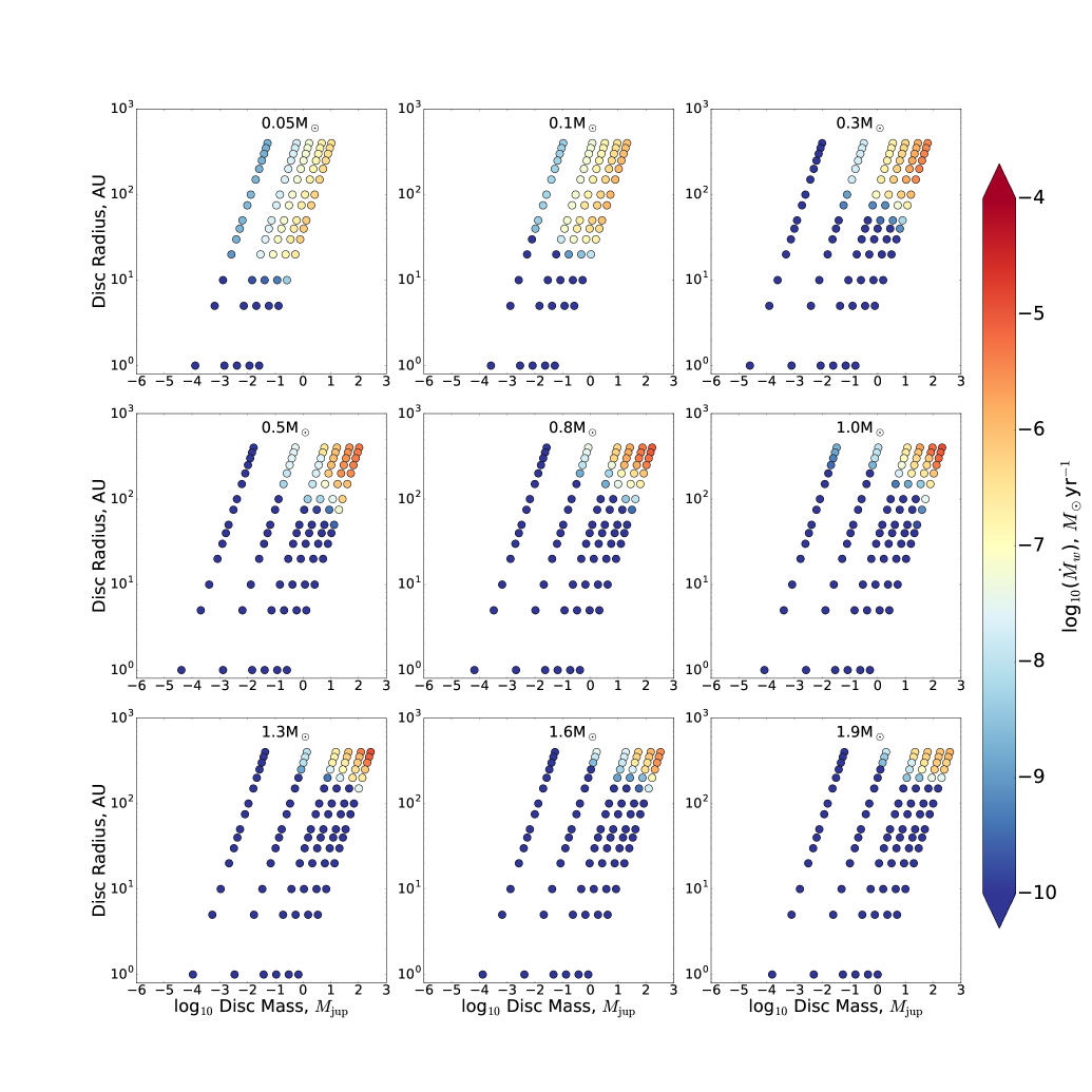
Figure 5: The mass loss rate for the 10 G₀ models over our entire parameter space, plotted as a function of disc mass and outer radius. The stellar mass in each case is denoted above each panel. Note that the grid has a floor value on the mass loss rate of $10^{-10}$ M_⊙ yr^-1

Figure 6: The mass loss rate for the $10^{2}$ G₀ models over our entire parameter space, plotted as a function of disc mass and outer radius. The stellar mass in each case is denoted above each panel. Note that the grid has a floor value on the mass loss rate of $10^{-10}$ M_⊙ yr^-1

Figure 7: The mass loss rate for the $10^{3}$ G₀ models over our entire parameter space, plotted as a function of disc mass and outer radius. The stellar mass in each case is denoted above each panel. Note that the grid has a floor value on the mass loss rate of $10^{-10}$ M_⊙ yr^-1

Figure 8: The mass loss rate for the $5\times 10^{3}$ G₀ models over our entire parameter space, plotted as a function of disc mass and outer radius. The stellar mass in each case is denoted above each panel. Note that the grid has a floor value on the mass loss rate of $10^{-10}$ M_⊙ yr^-1

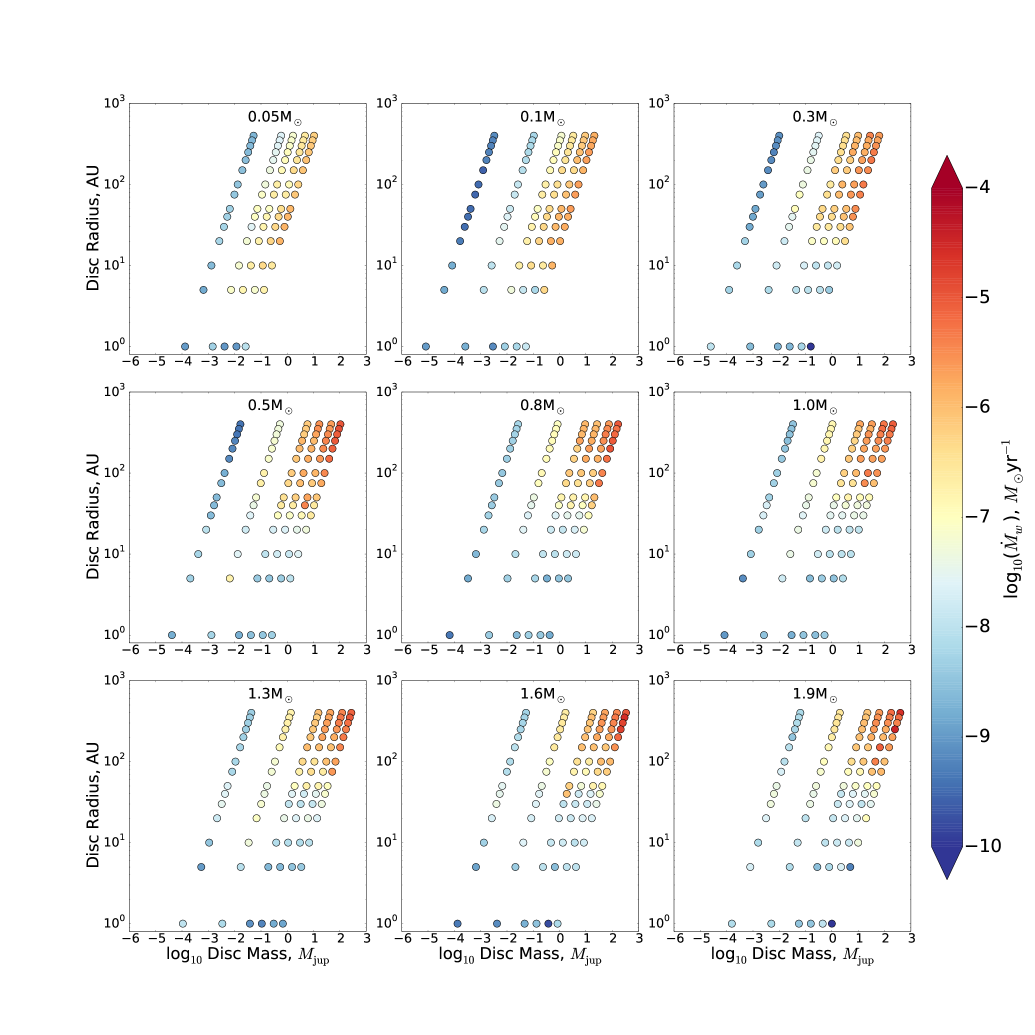
Figure 9: The mass loss rate for the $10^{4}$ G₀ models over our entire parameter space, plotted as a function of disc mass and outer radius. The stellar mass in each case is denoted above each panel. Note that the grid has a floor value on the mass loss rate of $10^{-10}$ M_⊙ yr^-1

References

- ALMA Partnership et al. (2015) ALMA Partnership Brogan C. L., Pérez L. M., Hunter T. R., Dent W. R. F., et al. 2015, ApJ, 808, L3
- Adams et al. (2004) Adams F. C., Hollenbach D., Laughlin G., Gorti U., 2004, ApJ, 611, 360
- Ali et al. (2018) Ali A., Harries T. J., Douglas T. A., 2018, MNRAS, 477, 5422
- Anderson et al. (2013) Anderson K. R., Adams F. C., Calvet N., 2013, ApJ, 774, 9
- Andrews (2015) Andrews S. M., 2015, PASP, 127, 961
- Ansdell et al. (2017) Ansdell M., Williams J. P., Manara C. F., Miotello A., Facchini S., van der Marel N., Testi L., van Dishoeck E. F., 2017, AJ, 153, 240
- Ansdell et al. (2018) Ansdell M., et al., 2018, ApJ, 859, 21
- Bisbas et al. (2015) Bisbas T. G., Haworth T. J., Barlow M. J., Viti S., Harries T. J., Bell T., Yates J. A., 2015, MNRAS, 454, 2828
- Cabrit et al. (2006) Cabrit S., Pety J., Pesenti N., Dougados C., 2006, A&A, 452, 897
- Churchwell et al. (1987) Churchwell E., Felli M., Wood D. O. S., Massi M., 1987, ApJ, 321, 516
- Cieza et al. (2017) Cieza L. A., Casassus S., Pérez S., Hales A., Cárcamo M., Ansdell M., et al. 2017, ApJ, 851, L23
- Clarke (2007) Clarke C. J., 2007, MNRAS, 376, 1350
- Clarke & Alexander (2016) Clarke C. J., Alexander R. D., 2016, MNRAS, 460, 3044
- Cleeves et al. (2016) Cleeves L. I., Öberg K. I., Wilner D. J., Huang J., Loomis R. A., Andrews S. M., Czekala I., 2016, ApJ, 832, 110
- Currie et al. (2015) Currie T., Cloutier R., Brittain S., Grady C., Burrows A., Muto T., Kenyon S. J., Kuchner M. J., 2015, The Astrophysical Journal Letters, 814, L27
- Dai et al. (2015) Dai F., Facchini S., Clarke C. J., Haworth T. J., 2015, MNRAS, 449, 1996
- Desidera & Barbieri (2007) Desidera S., Barbieri M., 2007, A&A, 462, 345
- Eisner et al. (2018) Eisner J. A., et al., 2018, ApJ, 860, 77
- Facchini et al. (2016) Facchini S., Clarke C. J., Bisbas T. G., 2016, MNRAS, 457, 3593
- Facchini et al. (2017) Facchini S., Birnstiel T., Bruderer S., van Dishoeck E. F., 2017, A&A, 605, A16
- Facchini et al. (2018) Facchini S., Juhász A., Lodato G., 2018, MNRAS, 473, 4459
- Fatuzzo & Adams (2008) Fatuzzo M., Adams F. C., 2008, ApJ, 675, 1361
- Fedele et al. (2018) Fedele D., et al., 2018, A&A, 610, A24
- Garufi et al. (2017) Garufi A., Benisty M., Stolker T., Avenhaus H., et al. 2017, The Messenger, 169, 32
- Geers et al. (2006) Geers V. C., et al., 2006, A&A, 459, 545
- Goldreich & Tremaine (1980) Goldreich P., Tremaine S., 1980, ApJ, 241, 425
- Gorti et al. (2015) Gorti U., Hollenbach D., Dullemond C. P., 2015, ApJ, 804, 29
- Guilloteau et al. (2011) Guilloteau S., Dutrey A., Piétu V., Boehler Y., 2011, A&A, 529, A105
- Habing (1968) Habing H. J., 1968, Bull. Astron. Inst. Netherlands, 19, 421
- Harries (2000) Harries T. J., 2000, MNRAS, 315, 722
- Haworth et al. (2015) Haworth T. J., Harries T. J., Acreman D. M., Bisbas T. G., 2015, MNRAS, 453, 2277
- Haworth et al. (2016a) Haworth T. J., Ilee J. D., Forgan D. H., Facchini S., Price D. J., et al. 2016a, Publ. Astron. Soc. Australia, 33, e053
- Haworth et al. (2016b) Haworth T. J., Boubert D., Facchini S., Bisbas T. G., Clarke C. J., 2016b, MNRAS, 463, 3616
- Haworth et al. (2017) Haworth T. J., Facchini S., Clarke C. J., Cleeves L. I., 2017, MNRAS, 468, L108
- Haworth et al. (2018) Haworth T. J., Facchini S., Clarke C. J., Mohanty S., 2018, MNRAS, 475, 5460
- Heiner & Vázquez-Semadeni (2013) Heiner J. S., Vázquez-Semadeni E., 2013, MNRAS, 429, 3584
- Henney & O’Dell (1999) Henney W. J., O’Dell C. R., 1999, AJ, 118, 2350
- Henney et al. (2002) Henney W. J., O’Dell C. R., Meaburn J., Garrington S. T., Lopez J. A., 2002, ApJ, 566, 315
- Hollenbach et al. (1994) Hollenbach D., Johnstone D., Lizano S., Shu F., 1994, ApJ, 428, 654
- Johnstone et al. (1998) Johnstone D., Hollenbach D., Bally J., 1998, ApJ, 499, 758
- Kalyaan et al. (2015) Kalyaan A., Desch S. J., Monga N., 2015, ApJ, 815, 112
- Kim et al. (2016) Kim J. S., Clarke C. J., Fang M., Facchini S., 2016, ApJ, 826, L15
- McCaughrean & O’dell (1996) McCaughrean M. J., O’dell C. R., 1996, AJ, 111, 1977
- McElroy et al. (2013) McElroy D., Walsh C., Markwick A. J., Cordiner M. A., Smith K., Millar T. J., 2013, A&A, 550, A36
- Morbidelli & Raymond (2016) Morbidelli A., Raymond S. N., 2016, Journal of Geophysical Research (Planets), 121, 1962
- Nakatani et al. (2018) Nakatani R., Hosokawa T., Yoshida N., Nomura H., Kuiper R., 2018, ApJ, 857, 57
- O’Dell (1998) O’Dell C. R., 1998, AJ, 115, 263
- O’Dell (2001) O’Dell C. R., 2001, AJ, 122, 2662
- Oliveira et al. (2010) Oliveira I., et al., 2010, ApJ, 714, 778
- Owen et al. (2012) Owen J. E., Clarke C. J., Ercolano B., 2012, MNRAS, 422, 1880
- Papaloizou & Pringle (1983) Papaloizou J. C. B., Pringle J. E., 1983, MNRAS, 202, 1181
- Parker (1965) Parker E. N., 1965, Space Sci. Rev., 4, 666
- Perez-Becker & Chiang (2011) Perez-Becker D., Chiang E., 2011, ApJ, 727, 2
- Pinte et al. (2018) Pinte C., et al., 2018, A&A, 609, A47
- Rapson et al. (2015) Rapson V. A., Kastner J. H., Millar-Blanchaer M. A., Dong R., 2015, The Astrophysical Journal Letters, 815, L26
- Ribas et al. (2015) Ribas Á., Bouy H., Merín B., 2015, A&A, 576, A52
- Rodriguez et al. (2018) Rodriguez J. E., et al., 2018, ApJ, 859, 150
- Scally & Clarke (2001) Scally A., Clarke C., 2001, MNRAS, 325, 449
- Sicilia-Aguilar et al. (2016) Sicilia-Aguilar A., et al., 2016, Publ. Astron. Soc. Australia, 33, e059
- Wang & Goodman (2017) Wang L., Goodman J., 2017, ApJ, 847, 11
- Williams & Cieza (2011) Williams J. P., Cieza L. A., 2011, ARA&A, 49, 67
- Winn & Fabrycky (2015) Winn J. N., Fabrycky D. C., 2015, ARA&A, 53, 409
- Winter et al. (2018a) Winter A. J., Clarke C. J., Rosotti G., Booth R. A., 2018a, MNRAS, 475, 2314
- Winter et al. (2018b) Winter A. J., Clarke C. J., Rosotti G., Ih J., Facchini S., Haworth T. J., 2018b, MNRAS, 478, 2700
- Zucker & Mazeh (2002) Zucker S., Mazeh T., 2002, ApJ, 568, L113
- de Gregorio-Monsalvo et al. (2013) de Gregorio-Monsalvo I., Ménard F., Dent W., Pinte C., et al. 2013, A&A, 557, A133
- van Dishoeck & Black (1986) van Dishoeck E. F., Black J. H., 1986, ApJS, 62, 109
- van Dishoeck & Black (1988) van Dishoeck E. F., Black J. H., 1988, ApJ, 334, 771
- van Leer (1979) van Leer B., 1979, Journal of Computational Physics, 32, 101