Analog of cosmological particle creation in electromagnetic waveguides

Abstract

We consider an electromagnetic waveguide with a time-dependent propagation speed $v(t)$ as an analog for cosmological particle creation. In contrast to most previous studies which focus on the number of particles produced, we calculate the corresponding two-point correlation function. For a small step-like variation $\delta v(t)$, this correlator displays characteristic signatures of particle pair creation. As another potential advantage, this observable is of first order in the perturbation $\delta v(t)$, whereas the particle number is second order in $\delta v(t)$ and thus stronger suppressed for small $\delta v(t)$.

I Introduction

Just a decade after Hubble’s discovery of cosmic expansion Hubble (1929), Schrödinger understood this mechanism to allow for particle creation out of the quantum vacuum Schrödinger (1939). Being one of the most startling predictions of quantum field theory in curved space-times, cosmological particle creation was further studied by Parker Parker (1968) and others (see also Birrell and Davies (1982)) in the late 1960’s. In the present universe, this effect is extremely tiny – but, according to our standard model of cosmology, it played an important role for the creation of seeds of structure formation during cosmic inflation Mukhanov et al. (1992). Signatures of this process can still be observed today in the anisotropies of the cosmic micro-wave background radiation.

As direct experimental tests of cosmological particle creation are probably out of reach, several laboratory analogs Unruh (1981); Visser (1998); Barceló et al. (2011) for quantum fields in expanding space-times have been proposed for various scenarios, including Bose-Einstein condensates Barceló et al. (2003); Fedichev and Fischer (2003); Fischer (2004); Fischer and Schützhold (2004); Jain et al. (2007); Prain et al. (2010); Neuenhahn and Marquardt (2015); Eckel et al. (2018), ion traps Alsing et al. (2005); Schützhold et al. (2007); Fey et al. (2018); Wittemer et al. (2019), and electromagnetic waveguides Lähteenmäki et al. (2013). In the following, we shall consider the latter system (see also Tian et al. (2017)), which has already been used to observe an analog of the closely related dynamical Casimir effect Schützhold et al. (1998); Johansson et al. (2009, 2010); Wilson et al. (2011); Lähteenmäki et al. (2013).

Instead of the often considered number of emerging particles, one can also study other observables, such as the two-point correlation function of the associated quantum field. For condensed-matter analogs of black-holes (see, e.g., Unruh (1981); Visser (1998); Schützhold and Unruh (2005); Barceló et al. (2011)), these correlations have already been studied in several works including Balbinot et al. (2008); Carusotto et al. (2008); Macher and Parentani (2009); Schützhold and Unruh (2010). In fact, the observation of analog Hawking radiation in Bose-Einstein condensates reported in Steinhauer (2016) was based on correlation measurements.

Cosmological particle creation does also generate characteristic signatures in the corresponding field correlations, see also Prain et al. (2010). Due to spatial homogeneity, particles are created in pairs with opposite momenta. When both particles of a pair arrive at two suitable detectors at different space or space-time points $(t_{1},x_{1})$ and $(t_{2},x_{2})$, the associated signals are clearly correlated.

In the following, we study two-point correlations in an electromagnetic waveguide with a time-dependent effective speed of light $v(t)$. Reducing this parameter $v(t)$ effectively increases all length scales in the set-up under consideration – in analogy to cosmic expansion. Therefore, laboratory systems with a varying speed of light $v(t)$ ought to produce photon pairs in perfect analogy to the mechanism of cosmological particle creation.

II Classical waveguide model

Previous research on circuit quantum electrodynamics has brought up various possible implementations of waveguides with tunable parameters, see, e.g., Nation et al. (2009); Castellanos-Beltran et al. (2008); Lähteenmäki et al. (2013); Tian et al. (2017); Navez et al. (2019). Although realistic experiments are often based on superconducting quantum interference devices (SQUIDS), they typically still correspond to effective circuit diagrams. In this work, we will focus on waveguide structures that can be modeled with the effective set-up illustrated in Fig. 1.

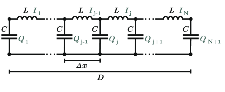
Figure 1: Illustration of an $LC$-circuit of length $D=N\,\Delta x$ that comprises $N$ discrete inductors and $N+1$ capacitors. The symbols $I_{j}$ and $Q_{j}$ denote the current in the $j$-th inductor and the charge on the $j$-th capacitor respectively.

Specifically, we consider an $LC$-circuit of total length $D$ which comprises $N+1$ capacitors with equal capacities $C$ and $N$ inductors with equal but time-dependent inductances $L(t)$. Denoting the current in the $j$-th inductor with the symbol $I_{j}$ and the charge on the $j$-th capacitor with $Q_{j}$, the Lagrangian of the set-up from Fig. 1 adopts the form

$$\begin{aligned} \mathfrak{L}(t)=\sum_{j=1}^{N+1}\frac{1}{2\;\!C}\;Q_{j}^{2}(t)-\sum_{j=1}^{N}\frac{1}{2}\;L(t)\;\!I_{j}^{2}(t)\text{.}\end{aligned}$$ (1)

Analogous to , we introduce a new generalized coordinate $\Phi_{j}(t)$ satisfying the relation $\dot{\Phi}_{j}(t)=Q_{j}/\sqrt{C\;\Delta x}$. Apart from this, we eliminate all currents $I_{j}$ in the above Lagrangian $\mathfrak{L}(t)$ with the second line of the classical Kirchhoff’s laws

$$\begin{aligned} &\dot{Q}_{j}\!\!\!&=\text{\;}&I_{j}-I_{j-1}\,,\\ &0\!\!\!&=\text{\;}&Q_{j}/C+\partial_{t}\left[L(t)I_{j}\right]-Q_{j+1}/C\,\text{.}\end{aligned}$$ (2)

Henceforth, we will further assume the length $\Delta x$ of each mesh in Fig. 1 to be significantly smaller than the characteristic wavelengths and the total length $D=N\Delta x$ of the waveguide. In the corresponding continuum limit of $\Delta x\rightarrow 0$ and $D=\text{const.}$, the Lagrangian $\mathfrak{L}(t)$ from equation (1) turns into the expression

$$\begin{aligned} \mathfrak{L}(t)=\frac{1}{2}\int_{0}^{D}\!\!\!\mathrm{dx}\left[\left[\dot{\Phi}(t,x)\right]^{2}-v^{2}(t)\left[\Phi^{\prime}(t,x)\right]^{2}\right]\text{,}\end{aligned}$$ (3)

where the quantity $v(t)=\Delta x/\sqrt{L(t)\,C}$ accounts for the effective speed of light inside the circuit .

Integrating the second line of equation (2) with respect to $t$ further yields a relation $I(t,x)\propto\Phi^{\prime}(t,x)$ for the electric current in the continuum limit. As the waveguide depicted in Fig. 1 is isolated at both ends, the generalized flux $\Phi(t,x)$ inherits Neumann boundary conditions $\Phi^{\prime}(t,0)=\Phi^{\prime}(t,D)=0$ $\forall\;t\in\mathbb{R}$ Note (1).

III Canonical quantization

In order to quantize the classical model from above, we follow the path of canonical quantization and obtain the Hamiltonian

$$\begin{aligned} \hat{\mathfrak{H}}(t)=\frac{1}{2}\int_{0}^{D}\!\!\!\mathrm{dx}\left[{\hat{\Pi}}^{2}(t,x)+v^{2}(t)\left[\hat{\Phi}^{\prime}(t,x)\right]^{2}\right]\end{aligned}$$ (4)

in which the operators $\hat{\Phi}(t,x)$ and $\hat{\Pi}(t,x)$ satisfy canonical commutation relations for a quantum field and its associated momentum.

The corresponding Heisenberg equations of motion can be combined to the wave equation

$$\begin{aligned} \ddot{\hat{\Phi}}(t,x)=\;v^{2}(t)\;\hat{\Phi}^{\prime\prime}(t,x)\text{.}\end{aligned}$$ (5)

Bearing in mind that the field $\hat{\Phi}(t,x)$ has to satisfy Neumann boundary conditions, the mode functions

$$\begin{aligned} &\Psi_{n=0}(x)\!\!\!&=&\,\,\sqrt{1/D}\\ &\Psi_{n>0}(x)\!\!\!&=&\,\,\sqrt{2/D}\cos{\left(\pi\,n\,x/D\right)}\end{aligned}$$ (6)

allow for a decomposition

$$\begin{aligned} \hat{\Phi}(t,x)=\sum_{n=0}^{\infty}\Psi_{n}(x)\;\hat{\varphi}_{n}(t)\end{aligned}$$ (7)

of the field operator $\hat{\Phi}(t,x)$, in which each term $\hat{\varphi}_{n}(t)$ constitutes a harmonic oscillator satisfying the differential equation

$$\begin{aligned} \ddot{\hat{\varphi}}_{n}(t)=-{\omega_{n}}^{2}(t)\;\hat{\varphi}_{n}(t)\text{\quad with \quad}\omega_{n}(t)=\frac{\pi n\,v(t)}{D}\,\text{.}\end{aligned}$$ (8)

IV Suddenly changing speed of light

IV.1 Operator solution for a step-like profile $\boldsymbol{v(t)}$

For a rapidly changing speed of light

$$\begin{aligned} v(t)=\begin{cases}v_{0}\text{,}&t<0\\ v_{1}\text{,}&t>0\text{,}\end{cases}\end{aligned}$$ (9)

each operator $\hat{\varphi}_{n}(t)$ adopts a piecewise representation

$$\begin{aligned} \hat{\varphi}_{n}(t<0)=\frac{1}{\sqrt{2\,\omega_{n}^{0}}}\left[\mathrm{e}^{-\mathrm{i}\,\omega_{n}^{0}t}\,\hat{a}_{n}+\mathrm{H.c.}\right]\\ \hat{\varphi}_{n}(t>0)=\frac{1}{\sqrt{2\,\omega_{n}^{1}}}\left[\mathrm{e}^{-\mathrm{i}\,\omega_{n}^{1}t}\,\hat{b}_{n}+\mathrm{H.c.}\right]\end{aligned}$$ (10)

with $\omega_{n}^{i}=\pi n\,v_{i}/D$, where the expressions $\hat{a}_{n}$ and $\hat{b}_{n}$ satisfy canonical commutation relations for two separate sets of bosonic annihilators.

The differential equation (8) requires each operator $\hat{\varphi}_{n}(t)$ and its temporal derivative $\partial_{t}\hat{\varphi}_{n}(t)$ to be continuous at $t=0$, which implies the connection

$$\begin{aligned} \hat{b}_{n}=\frac{1}{2}\sqrt{\frac{v_{1}}{v_{0}}}\left[\left(1-\frac{v_{0}}{v_{1}}\right)\hat{a}^{\dagger}_{n}+\left(1+\frac{v_{0}}{v_{1}}\right)\hat{a}_{n}\right]\text{.}\end{aligned}$$ (11)

IV.2 Particle creation

Based on the previous finding (11), we can easily study how expectation values for the particle number operator

$$\begin{aligned} \hat{N}_{n}(t)=\begin{cases}\hat{a}^{\dagger}_{n}\,\hat{a}_{n}\text{,}&t<0\\[5.0pt] \hat{b}^{\dagger}_{n}\,\hat{b}_{n}\text{,}&t>0\end{cases}\end{aligned}$$ (12)

of the $n$-th mode evolve with time.

In order to demonstrate the occurrence of particle production, we use the Heisenberg picture and study the expectation value $\bra{0}\hat{N}_{n}(t)\ket{0}$ for the initial vacuum state $\ket{0}$. Since this state satisfies the relation $\hat{a}_{n}\ket{0}=0$ for all modes $n$, the number of photons inside the waveguide vanishes at all negative times. In the regime of $t>0$, the particle number adopts the finite and constant value of $(v_{1}-v_{0})^{2}/(4\,v_{0}\,v_{1})$ for all modes $n$ (see also Tian et al. (2017)).

Consequently, particle creation for the sudden step $v(t)$ from equation (9) occurs at the sharp instant of $t=0$ and uniformly affects all modes . However, the number of particles produced is of second order in the perturbation $\delta v=v_{1}-v_{0}$ which might constitute a challenge for future experiments with small $\delta v$.

IV.3 Two-point correlation for the operator $\boldsymbol{\hat{\Phi}(t,x)}$

In case of a sharp step-function $v(t)$, the two-point correlation for the full field $\hat{\Phi}(t,x)$ can be evaluated analytically. In order to extract real results, we focus on the expression

$$\begin{aligned} \kappa(t_{1},x_{1},t_{2},x_{2})=\mathrm{Re}\left[{\bra{0}\hat{\Phi}(t_{1},x_{1})\;\!\hat{\Phi}(t_{2},x_{2})\ket{0}}\right]\!-\chi_{\infty}\end{aligned}$$ (13)

which has been symmetrized with respect to an exchange of both space-time points $(t_{1},x_{1})$ and $(t_{2},x_{2})$. We further assume the term $\chi_{\infty}$ to compensate for the infinite but constant contribution of the infrared divergence associated with the lowest $(n=0)$-mode.

Exact analytic results for the correlation $\kappa(t_{1},x_{1},t_{2},x_{2})$ are calculated in Appendix A. For all pairs of fixed times $t_{1}$ and $t_{2}$, the expression $\kappa(t_{1},x_{1},t_{2},x_{2})$ has logarithmic singularities along characteristic lines in the $(x_{1},x_{2})$-plane.

IV.3.1 Two-point correlation for negative $t_{1}$ and $t_{2}$

If both times $t_{1}$ and $t_{2}$ are negative, the two-point correlation $\kappa(t_{1}\leq 0,x_{1},t_{2}\leq 0,x_{2})$ given in Appendix A diverges to positive infinity under the condition

$$\begin{aligned} x_{1}+s_{1}\,x_{2}-s_{2}\,v_{0}\,(t_{1}-t_{2})=2\,D\,m\end{aligned}$$ (14)

with $s_{1},s_{2}\in\{\pm 1\}$ and $m\in\mathbb{Z}$.

This identity just accounts for the standard light-cone singularities (possibly including reflections at the boundaries) in the initial vacuum state, see Figs. 2 and 3.

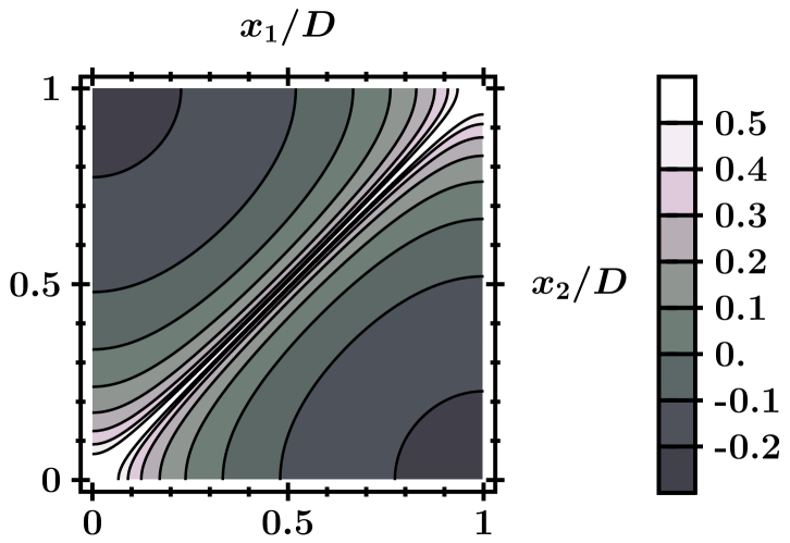
Figure 2: Rescaled equal-time correlation $v_{0}\,\kappa(t_{1},x_{1},t_{1},x_{2})$ plotted for an arbitrary argument $t_{1}\leq 0$. Singularities just occur along the line with $x_{1}=x_{2}$.

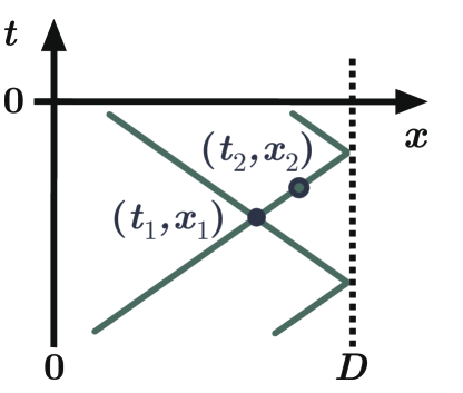
Figure 3: Worldlines for two different ‘signals‘ passing through a given space-time point $(t_{1},x_{1})$ at velocities of absolute value $v_{0}$. For all points $(t_{2},x_{2})$ on either worldline, the correlation function $\kappa(t_{1}\leq 0,x_{1},t_{2}\leq 0,x_{2})$ diverges.

IV.3.2 Two-point correlation for positive $t_{1}$ and $t_{2}$

For positive times $t_{1}$ and $t_{2}$, the expression $\kappa(t_{1}>0,x_{1},t_{2}>0,x_{2})$ calculated in Appendix A adopts singularities under conditions of two different types

$$\begin{aligned} &x_{1}+s_{1}\,x_{2}-s_{2}\,v_{1}\,(t_{1}-t_{2})=2\,D\,m\\ &x_{1}+s_{1}\,x_{2}-s_{2}\,v_{1}\,(t_{1}+t_{2})=2\,D\,m\text{.}\end{aligned}$$ (15)

Except for a modified speed of light, the first identity from equation (15) has the same form as the corresponding expression (14) for negative times $t_{1}$ and $t_{2}$. It thus also describes usual light-cone singularities.

In contrast, the second type of singularities stems from the creation of particle pairs at $t=0$. As one indication, the second line of equation (15) is not invariant under time translation. As another indication, the corresponding pre-factors in the result $\kappa(t_{1}>0,x_{1},t_{2}>0,x_{2})$ from Appendix A scale linearly with the perturbation $\delta v=v_{1}-v_{0}$. As an intuitive picture, one can imagine pair creation at the sharp time $t=0$ and some random position $x_{0}$, where the produced particles propagate with opposite velocities $\pm v_{1}$. The condition $x_{2}-x_{1}=v_{1}(t_{1}+t_{2})$ associated with this configuration is illustrated in Fig. 4.

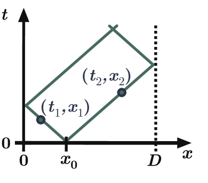
Figure 4: Worldlines for a photon pair which is produced at an arbitrary position $x_{0}$ and the sharp time $t=0$. For all points $(t_{1},x_{1})$ and $(t_{2},x_{2})$ located on opposite worldlines, the correlation function $\kappa(t_{1}>0,x_{1},t_{2}>0,x_{2})$ has singularities characterized by the second line of equation (15).

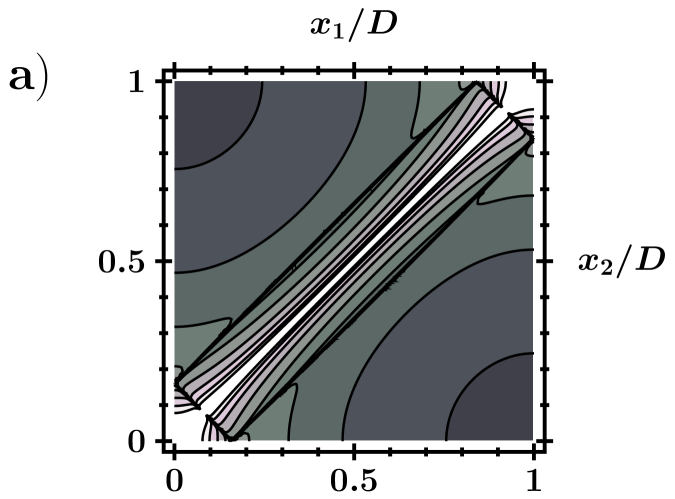
(a)

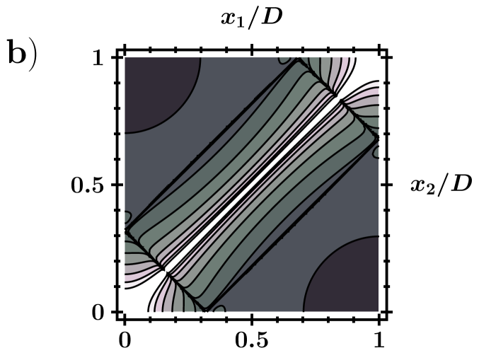
(b)

Figure 5: Rescaled equal-time correlation $v_{0}\,\kappa(t_{1},x_{1},t_{1},x_{2})$ plotted for two different arguments $t_{1}>0$ and velocities $v_{0}=D$ as well as $v_{1}=0.8\;D$. The parameter $t_{1}$ adopts the value $0.1$ in plot a) and $0.2$ in plot b).
Singularities described by the second line of equation (15) occur along the black rectangular structure visible in both plots. The colour scale is consistent with Fig. 2.

Fig. 5 provides plots of the correlation function $\kappa(t_{1},x_{1},t_{2},x_{2})$ for two fixed pairs of identical positive times $t_{1}=t_{2}$. The singularities characterized by the second line of equation (15) occur along the black rectangle appearing in both of these plots. As a function of time, the corners of this structure continuously move along the boundaries of the domain $\left[0,D\right]^{2}$.

Note that the sign of correlations along the rectangular pattern from Fig. 5 depends on the ratio of both velocities $v_{0}$ and $v_{1}$. We obtain divergences to negative infinity if $v_{0}>v_{1}$, and to positive infinity in case of $v_{0}<v_{1}$. Thus, the former case $v_{0}>v_{1}$ offers the advantage that singularities due to pair production are well-distinguishable from light-cone singularities.

IV.3.3 Two-point correlation for $t_{1}$ and $t_{2}$ having opposite signs

If the times $t_{1}$ and $t_{2}$ differ in sign, we obtain singularities of the same types as in the previous paragraph. Given the exemplary case of $t_{1}<0$ and $t_{2}>0$, divergences occur under the specific conditions

$$\begin{aligned} x_{1}+s_{1}\,x_{2}-s_{2}\,(v_{0}\,t_{1}-&\,v_{1}\,t_{2})=2\,D\,m\\ x_{1}+s_{1}\,x_{2}-s_{2}\,(v_{0}\,t_{1}+&\,v_{1}\,t_{2})=2\,D\,m\text{.}\end{aligned}$$ (16)

Taking the change of propagation velocity at $t=0$ into account, singularities specified by the first line of equation (16) can be associated with the light-cone once again.

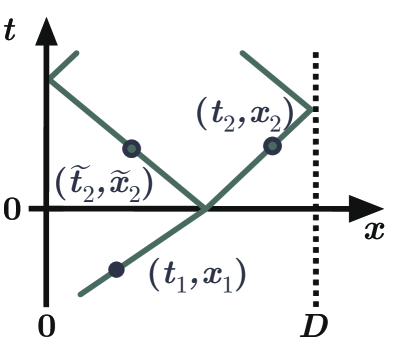
Figure 6: Two possible world-lines for an initial quantum fluctuation passing through a space-time point $(t_{1},x_{1})$ with $t_{1}<0$. The condition in the first line of equation (16) is satisfied for all points $(t_{2}>0,x_{2})$ that are located on the right branch of the depicted light-cone. The second type of singularities emerges for those points $(\tilde{t}_{2}>0,\tilde{x}_{2})$ which belong to the other worldline illustrated above.

On the other hand, the second line of equation (16) indicates that quantum vacuum fluctuations propagating at an initial speed of either $+v_{0}$ or $-v_{0}$ are also partly reflected at the time $t=0$ and afterwards propagate with the new velocity $-v_{1}$ or $+v_{1}$ respectively. An illustration of both possible world-lines emerging from such a partial reflection is provided in Fig. 6. The splitting of initial fluctuations into superpositions of left- and right-moving components corresponds to the mixing of initial creation and annihilation operators $\hat{a}^{\dagger}_{n}$ and $\hat{a}_{n}$ in the new annihilators $\hat{b}_{n}$. Since this combination of terms $\hat{a}^{\dagger}_{n}$ and $\hat{a}_{n}$ is responsible for the occurrence of particle production, the partial reflections encoded in equation (16) illustrate that pair creation originates from fluctuations that have already been present at times $t<0$.

V Continuously changing speed

In order to assess whether the singularities obtained in Sect. IV also arise for smooth profiles $v(t)$, we repeat the previous calculations for a continuous function

$$\begin{aligned} v^{2}(t)=\gamma_{-}\tanh{\!(t/\tau)}+\gamma_{+}\text{\quad with \quad\,}\gamma_{\pm}=\frac{v_{1}^{2}\pm v_{0}^{2}}{2}\text{,}\end{aligned}$$ (17)

where $\tau$ measures the finite time of change.

Particle production in this modified set-up can be examined analogous to Sect. 3.4 of Ref. Birrell and Davies (1982) (see also Sauter (1932) for technical details). Again, we study the expression $\kappa(t_{1},x_{1},t_{2},x_{2})$ and analyze its behavior along the characteristic lines specified by equation (15). This involves several approximations that are further discussed in Appendix B.

V.1 Operator solution for a smooth step $\boldsymbol{v(t)}$

For the continuous profile $v^{2}(t)$ from equation (17), solutions $\hat{\varphi}_{n}(t)$ of the differential equation (8) generally have non-trivial time dependencies. However, in the limiting cases of $t\rightarrow\pm\infty$, the operators $\hat{\varphi}_{n}(t)$ still adopt asymptotic representations equivalent to the result (10) for a sharp step. Explicit calculations reveal the specific connection

$$\begin{aligned} \hat{b}_{n}=\zeta_{n}^{(+)}\,\hat{a}_{n}\,\,+\,\,\zeta_{n}^{(-)}\,\hat{a}^{\dagger}_{n}\end{aligned}$$ (18)

with

$$\begin{aligned} &\zeta_{n}^{(\pm)}\text{\!\!\!}&=\text{\;}&\sqrt{\frac{w^{1}_{n}}{w^{0}_{n}}}\,\frac{\Gamma\!\left[1\mp\mathrm{i}\,w^{0}_{n}\tau\right]\,\Gamma\!\left[-\,\mathrm{i}\,w^{1}_{n}\tau\right]}{\Gamma\!\left[1\mp\frac{\mathrm{i}}{2}\,(w^{0}_{n}\pm w^{1}_{n})\,\tau\right]\,\Gamma\!\left[\mp\frac{\mathrm{i}}{2}\,(w^{0}_{n}\pm w^{1}_{n})\,\tau\right]}\end{aligned}$$ (19)

between the asymptotic annihilator $\hat{b}_{n}$ after changing the speed of light and the corresponding initial ladder operators $\hat{a}_{n}$ and $\hat{a}_{n}^{\dagger}$, see also Birrell and Davies (1982).

V.2 Particle creation for a smooth step $\boldsymbol{v(t)}$

By evaluating expectation values $\bra{0}\hat{b}^{\dagger}_{n}\,\hat{b}_{n}\ket{0}$ for the initial vacuum $\ket{0}$, we find the number of photons created in the $n$-th mode to adopt the well-known value Tian et al. (2017); Birrell and Davies (1982)

$$\begin{aligned} \bra{0}\hat{b}^{\dagger}_{n}\,\hat{b}_{n}\ket{0}=\left|\zeta_{n}^{(-)}\right|^{2}=\frac{\sinh^{2}{\left[\frac{\pi}{2}\;\!(\omega_{n}^{0}-\omega_{n}^{1})\;\!\tau\right]}}{\sinh{\left[\pi\;\!\omega_{n}^{0}\;\!\tau\right]}\sinh{\left[\pi\;\!\omega_{n}^{1}\;\!\tau\right]}}\end{aligned}$$ (20)

for times $t\rightarrow\infty$ . For sharp step-functions with $\tau\to 0$ or in case of $n=0$, the above result reduces to the familiar expression $(v_{0}-v_{1})^{2}/(4\,v_{0}\,v_{1})$. On the other hand, the photon number $\bra{0}\hat{b}^{\dagger}_{n}\,\hat{b}_{n}\ket{0}$ undergoes exponential decay for $n\rightarrow\infty$, which results in a suppression of particle creation at short wavelengths $\lambda_{n}=2D/n$ . Apart from this, particle production also vanishes if the continuous step $v(t)$ from equation (17) has a broad temporal width $\tau\rightarrow\infty$.

V.3 Two-point correlation after a smooth step $\boldsymbol{v(t)}$

Unlike a sudden step-function $v(t)$, the continuous profile $v(t)$ from equation (17) does not yield a compact expression for the two-point correlation $\kappa(t_{1},x_{1},t_{2},x_{2})$. However, for sufficiently large times $t_{1}$ and $t_{2}\gg\tau$, further discussions in Appendix B provide an approximate result $\kappa(t_{1},x_{1},t_{2},x_{2})$ that correctly includes the contributions of modes with large $n$. Since all singularities of the quantity $\kappa(t_{1},x_{1},t_{2},x_{2})$ arise from high modes approaching $n\rightarrow\infty$, the large-$n$ approximation in Appendix B clearly reveals whether a smooth step $v(t)$ yields the same divergent contributions as its discontinuous counterpart from equation (9).

As expected, we find the two-point correlation $\kappa(t_{1},x_{1},t_{2},x_{2})$ to still diverge under the light-cone conditions

$$\begin{aligned} x_{1}+s_{1}\,x_{2}-s_{2}\,v_{1}\,(t_{1}-t_{2})=2\,D\,m\text{,}\end{aligned}$$ (21)

while the additional singularities due to pair creation

$$\begin{aligned} x_{1}+s_{1}\,x_{2}-s_{2}\,v_{1}\,(t_{1}+t_{2})=2\,D\,m\end{aligned}$$ (22)

from Sect. IV are smoothened out for continuous profiles $v(t)$. This can be explained by the fact that particle creation can no longer be associated with a sharp point of time.

VI Conclusion

As a laboratory analog for cosmological particle creation, we have considered a waveguide with a time-dependent speed of light $v(t)$ and calculated the two-point correlation $\kappa(t_{1},x_{1},t_{2},x_{2})$ for the generalized flux variable $\hat{\Phi}(t,x)$. First, we studied a sudden step function $v(t)$. In addition to the usual light-cone singularities (possibly including reflections at the boundaries), we found a distinctive pattern of logarithmic singularities in $\kappa(t_{1},x_{1},t_{2},x_{2})$ which clearly reflects the dynamics of pair creation occurring at a sharp instant of time. If we replace the sudden step in $v(t)$ by a smooth profile, those additional singularities are smoothened out. Nevertheless, the correlation $\kappa(t_{1},x_{1},t_{2},x_{2})$ displays distinctive signatures of pair creation, which could be observed experimentally.

In contrast to the number of particles produced (see, e.g., Tian et al. (2017)), the imprint of pair creation onto the correlation function $\kappa(t_{1},x_{1},t_{2},x_{2})$ is of first order in the perturbation $\delta v=v_{1}-v_{0}$. Therefore, we propose that measuring two-point correlations instead of particle numbers may enhance the chances for observing analog cosmological particle creation in future experiments with tunable waveguides.

Appendix A Calculation of the symmetrized two-point correlation for a rapid step $\boldsymbol{v(t)}$

In order to work out the symmetrized two-point correlation $\kappa(t_{1},x_{1},t_{2},x_{2})$ for a step-like profile $v(t)$, we insert the findings (7) and (10) into equation (13). After evaluating all quantum mechanical expectation values, elementary trigonometric identities can be used to rearrange the function $\kappa(t_{1},x_{1},t_{2},x_{2})$ into a sum containing multiple expressions of the characteristic shape

$$\begin{aligned} \sum_{n=1}^{\infty}\frac{p^{n}\cos{\left(n\,\xi\right)}}{n}=-\frac{1}{2}\ln{\left[1-2\,p\cos{\left(\xi\right)}+p^{2}\right]}\text{,}&&p^{2}\leq 1\text{,}\end{aligned}$$ (23)

with here $p=1$, where the result on the right-hand side has been taken from Eq. (1.448) in Ref. Gradshteyn and Ryzhik (2015).

Typical arguments $\xi$ occurring in terms of the specific shape (23) can be abbreviated with a symbol

$$\begin{aligned} \xi^{(v_{i},v_{j}|\pm)}_{s_{1},s_{2}}&(t_{1},x_{1},t_{2},x_{2})\\ &=\frac{\pi}{D}\left[x_{1}+s_{1}\,x_{2}-s_{2}\,(v_{i}\,t_{1}\pm v_{j}\,t_{2})\right]\end{aligned}$$ (24)

in which the indices $s_{1}$ and $s_{2}\in\{\pm 1\}$ constitute placeholders for two variable signs.

By applying the previous considerations to expressions $\kappa(t_{1},x_{1},t_{2},x_{2})$ with different combinations of signs $\mathrm{sgn}(t_{1})$ and $\mathrm{sgn}(t_{2})$, we obtain the specific results

$$\begin{aligned} &\kappa(t_{1}\leq 0,x_{1},t_{2}\leq 0,x_{2})=\!-\frac{1}{8\pi\,v_{0}}\,\\ &\text{\qquad\qquad}\times\sum_{s_{i}=\pm 1}\ln{\!\left[2-2\cos{\!\left[\xi^{(v_{0},v_{0}|-)}_{s_{1},s_{2}}(t_{1},x_{1},t_{2},x_{2})\right]}\right]}\text{,}\end{aligned}$$ (25)

$$\begin{aligned} &\kappa(t_{1}>0,x_{1},t_{2}>0,x_{2})=\!-\frac{1}{16\pi\,v_{0}}\sum_{\gamma=\pm 1}\left[1-\gamma\,\frac{{v_{0}}^{2}}{{v_{1}}^{2}}\right]\\ &\text{\qquad\qquad\;\;}\times\sum_{s_{i}=\pm 1}\ln{\!\left[2-2\cos{\!\left[\xi^{(v_{1},v_{1}|\gamma)}_{s_{1},s_{2}}(t_{1},x_{1},t_{2},x_{2})\right]}\right]}\end{aligned}$$ (26)

and

$$\begin{aligned} &\kappa(t_{1}\leq 0,x_{1},t_{2}>0,x_{2})=\!-\frac{1}{16\pi\,v_{0}}\sum_{\gamma=\pm 1}\left[1-\gamma\,\frac{{v_{0}}}{{v_{1}}}\right]\\ &\text{\qquad\qquad\;\;}\times\sum_{s_{i}=\pm 1}\ln{\!\left[2-2\cos{\!\left[\xi^{(v_{0},v_{1}|\gamma)}_{s_{1},s_{2}}(t_{1},x_{1},t_{2},x_{2})\right]}\right]}\text{.}\end{aligned}$$ (27)

For arbitrary fixed arguments $t_{1}$ and $t_{2}$, the above findings (25) to (27) have logarithmic singularities along characteristic lines in the $(x_{1},x_{2})$-plane. More specifically, such singularities arise if the respective term $\xi^{(v_{0},v_{0}|-)}_{s_{1},s_{2}}(t_{1},x_{1},t_{2},x_{2})$, $\xi^{(v_{1},v_{1}|\gamma)}_{s_{1},s_{2}}(t_{1},x_{1},t_{2},x_{2})$ or $\xi^{(v_{0},v_{1}|\gamma)}_{s_{1},s_{2}}(t_{1},x_{1},t_{2},x_{2})$ corresponds to an integer multiple of $2\pi$.

Appendix B Approximate result for the symmetrized two-point correlation after a smooth step $\boldsymbol{v(t)}$

B.0.1 General structure of the two-point correlation for large times $t_{1}$, $t_{2}\gg\tau$

For times $t\gg\tau$ located after the smooth step $v(t)$ from Sect. V, the full quantum field $\hat{\Phi}(t,x)$ adopts the asymptotic representation

$$\begin{aligned} &\hat{\Phi}(t\gg\tau,x)\text{\!\!\!}&=\;&\sum_{n=0}^{\infty}\frac{\Psi_{n}(x)}{\sqrt{2\,\omega_{n}^{1}}}\left[\mathrm{e}^{-\mathrm{i}\,\omega_{n}^{1}t}\,\hat{b}_{n}+\mathrm{H.c.}\right]\end{aligned}$$ (28)

in which the terms $\hat{b}_{n}$ are given by equation (18).

After inserting the above finding into the symmetrized correlation function (13), the identities already given in footnote Note (4) can be used to extract the result

$$\begin{aligned} \kappa(t_{1},x_{1},t_{2},x_{2})=\kappa_{\mathrm{A}}(t_{1},x_{1},t_{2},x_{2})+\kappa_{\mathrm{B}}(t_{1},x_{1},t_{2},x_{2})\end{aligned}$$ (29)

with

$$\begin{aligned} &\kappa_{\mathrm{A}}&\text{\!\!\!}=\;&\sum_{n=1}^{\infty}\frac{1}{2\,\omega_{n}^{1}}\,\Psi_{n}(x_{1})\,\Psi_{n}(x_{2})\,\cos{\left[\omega_{n}^{1}(t_{1}-t_{2})\right]}\\ &&\times\text{\,}&\frac{\sinh^{2}{\!\left[\frac{\pi}{2}(\omega_{n}^{0}+\omega_{n}^{1})\,\tau\right]}+\sinh^{2}{\!\left[\frac{\pi}{2}(\omega_{n}^{0}-\omega_{n}^{1})\,\tau\right]}}{\sinh{\!\left[\pi\,\omega_{n}^{0}\,\tau\right]}\sinh{\!\left[\pi\,\omega_{n}^{1}\,\tau\right]}}\end{aligned}$$ (30)

and

$$\begin{aligned} &\kappa_{\mathrm{B}}=\sum_{n=1}^{\infty}\frac{4\pi}{\left[(\omega_{n}^{0})^{2}-(\omega_{n}^{1})^{2}\right]\tau}\,\Psi_{n}(x_{1})\,\Psi_{n}(x_{2})\\ &\text{\quad}\times\,\mathrm{Re}\Bigg{[}\frac{\mathrm{e}^{-\mathrm{i}\,\omega_{n}^{1}\,(t_{1}+t_{2})}}{\sinh{\!\left(\pi\;\!\omega_{n}^{0}\;\!\tau\right)}}\left(\frac{\Gamma{\!\left[-\mathrm{i}\,\omega_{n}^{1}\,\tau\right]}}{\Gamma{\!\left[-\frac{\mathrm{i}\left(\omega_{n}^{0}+\omega_{n}^{1}\right)\tau}{2}\right]}\Gamma{\!\left[\frac{\mathrm{i}\left(\omega_{n}^{0}-\omega_{n}^{1}\right)\tau}{2}\right]}}\right)^{2}\Bigg{]}\text{.}\end{aligned}$$ (31)

B.0.2 Expansions allowing for an explicit evaluation

As both expressions $\kappa_{\mathrm{A}}$ and $\kappa_{\mathrm{B}}$ involve sums that lack straightforward analytic solutions, the following studies rely on approximations of the respective summands. In order to assess whether the two-point correlation $\kappa(t_{1},x_{1},t_{2},x_{2})$ after a smooth step $v(t)$ acquires the same singularities as the corresponding expression (26) for a rapidly changing speed of light, it is sufficient to examine the contributions of modes with large indices $n\rightarrow\infty$.

Based on the asymptotic expansion

$$\begin{aligned} \sinh{\pi x}\sim\mathrm{e}^{\pi x}/2\text{\qquad for }x\rightarrow\infty\end{aligned}$$ (32)

and the Stirling formula

$$\begin{aligned} \Gamma(z)\sim\sqrt{2\pi}\,\mathrm{e}^{-z}\,z^{z-1/2}\text{\qquad for }|z|\rightarrow\infty\text{,}\end{aligned}$$ (33)

we can significantly simplify both expressions (30) and (31).

Numerical studies reveal that the relative error associated with the approximation (32) is negligibly small for all arguments $x\geq 1$. Apart from this, the Stirling formula (33) also yields at least qualitatively reliable results for all purely imaginary arguments $z=\mathrm{i}x$ with $|x|>1$.

Bearing in mind the relation $\omega_{n}^{i}=\pi n\,v_{i}/D$, the expansions (32) and (33) are clearly applicable to all summands in the expressions $\kappa_{\mathrm{A}}$ and $\kappa_{\mathrm{B}}$ that have sufficiently large indices $n$. Moreover, they even hold for smaller integers $n\gtrsim 1$ if the step-width $\tau$ of the continuous profile $v(t)$ exceeds the characteristic times $D/(\pi v_{0})$, $D/(\pi v_{1})$ and $2D/|\pi(v_{0}-v_{1})|$.

For the exemplary set-up studied in Ref. Lähteenmäki et al. (2013), the values $D=$4\text{\,}\mathrm{m}\mathrm{m}$$ and $v_{0}=0.5\,c_{0}$ constitute realistic experimental parameters with $c_{0}$ denoting the vacuum speed of light. If we further assume $v_{1}=0.45\,c_{0}$, the asymptotic expansions (32) and (33) hold for all indices $n\in\mathbb{N}$ as long as $\tau\geq$1.7\text{\times}{10}^{-10}\text{\,}\mathrm{s}$$.

In the opposite case of $\tau$ violating the above requirements, the subsequent results contain incorrect contributions for modes with small indices $n$. Nevertheless, any conclusions concerning the appearance of singularities remain valid even if the underlying approximations are unreliable for low integers $n$.

B.0.3 Approximate result for the term $\kappa_{\mathrm{A}}(t_{1},x_{1},t_{2},x_{2})$

By applying the asymptotic expansion (32) to each summand of equation (30), we obtain the approximate result

$$\begin{aligned} &\kappa_{\mathrm{A}}&\text{\!\!\!}\approx\;&\sum_{n=1}^{\infty}\frac{\Psi_{n}(x_{1})\,\Psi_{n}(x_{2})}{2\;\!\omega_{n}^{1}}\,\cos{\left[\omega_{n}^{1}\,(t_{1}-t_{2})\right]}\\ &&&\text{\qquad\qquad\qquad\;\;}\times\left[1+\mathrm{e}^{-2\pi\min{\left\{\omega_{n}^{0},\omega_{n}^{1}\right\}}\,\tau}\right]\end{aligned}$$ (34)

that can be further simplified analogous to Appendix A.

More specifically, we expand the square brackets in the last term of equation (34), use the identity (23) with $p_{1}=1$ or $p_{2}=\exp{\left[-2\,\pi^{2}\,\min{\left\{v_{0},v_{1}\right\}}\,\tau/D)\right]}$ respectively and finally retain the expression

$$\begin{aligned} &\kappa_{\mathrm{A}}&\text{\!\!\!}\approx\;&-\frac{1}{8\pi\,v_{1}}\;\sum_{k=1,2}\;\sum_{s_{i}=\pm 1}\\ &&&\times\ln{\!\left[1-2\,p_{k}\cos{\!\left[\xi^{(v_{1},v_{1}|-)}_{s_{1},s_{2}}(t_{1},x_{1},t_{2},x_{2})\right]}+p_{k}^{2}\right]}\text{.}\end{aligned}$$ (35)

The $(k\!=\!1)$-contribution to the latter result obviously resembles the $(\gamma\!=\!-1)$-terms in the corresponding function $\kappa(t_{1}>0,x_{1},t_{2}>0,x_{2})$ from Appendix A. Therefore, the expression $\kappa_{\mathrm{A}}(t_{1},x_{1},t_{2},x_{2})$ similarly adopts singularities under the condition

$$\begin{aligned} x_{1}+s_{1}\,x_{2}-s_{2}\,v_{1}\,(t_{1}-t_{2})=2\,D\,m\text{.}\end{aligned}$$ (36)

On the other hand, all terms satisfying $k\!=\!2$ remain finite for arbitrary combinations of space-time points $(t_{1},x_{1})$ and $(t_{2},x_{2})$.

B.0.4 Approximate result for the term $\kappa_{\mathrm{B}}(t_{1},x_{1},t_{2},x_{2})$

Based on the Stirling formula (33), the squared parentheses in equation (31) can be approximated according to

$$\begin{aligned} &\left(\frac{\Gamma{\!\left[-\mathrm{i}\,\omega_{n}^{1}\,\tau\right]}}{\Gamma{\!\left[-\frac{\mathrm{i}\left(\omega_{n}^{0}+\omega_{n}^{1}\right)\tau}{2}\right]}\Gamma{\!\left[\frac{\mathrm{i}\left(\omega_{n}^{0}-\omega_{n}^{1}\right)\tau}{2}\right]}}\right)^{2}\\ &\text{\qquad\quad}\approx\text{\,}\frac{\mathrm{i}\,n\,\tau}{8\,D}\frac{\left(v_{0}^{2}-v_{1}^{2}\right)}{v_{1}}\mathrm{e}^{\frac{\pi^{2}\,\tau}{D}\,n\,(v_{0}-v_{1})\,\Theta(v_{0}-v_{1})}\\ &\text{\qquad\qquad\quad}\times\mathrm{e}^{-\mathrm{i}\frac{\pi\,n\,\tau}{D}\left[v_{0}\ln{\left(\frac{\left|v_{0}-v_{1}\right|}{v_{0}+v_{1}}\right)}+v_{1}\ln{\left(\frac{4v_{1}^{2}}{\left|v_{0}^{2}-v_{1}^{2}\right|}\right)}\right]}\text{,}\end{aligned}$$ (37)

where the symbol $\Theta$ denotes the Heaviside-function.

If we likewise replace the factor $\sinh{\!\left(\pi\,\omega_{n}^{0}\tau\right)}$ by means of equation (32), the resulting expression $\kappa_{\mathrm{B}}$ can be further reduced to the form

$$\begin{aligned} \kappa_{\mathrm{B}}\,&\approx\sum_{s_{i}\in\left\{\pm 1\right\}}\sum_{n=1}^{\infty}-\frac{s_{2}}{2\,\pi\,v_{1}}\\ &\times\,\frac{\mathrm{e}^{-\frac{\pi^{2}n\,\tau}{D}\min{\left\{v_{0},v_{1}\right\}}}}{n}\sin{\left[n\,\tilde{\xi}_{s_{1},s_{2}}(t_{1},x_{1},t_{2},x_{2})\right]}\end{aligned}$$ (38)

with

$$\begin{aligned} &\tilde{\xi}_{s_{1},s_{2}}(t_{1},x_{1},t_{2},x_{2})=\frac{\pi}{D}\bigg{[}x_{1}+s_{1}\,x_{2}-s_{2}\,v_{1}\,(t_{1}+t_{2})\\ &\text{\qquad\qquad}-s_{2}\,v_{0}\,\tau\,\ln{\left(\frac{\left|v_{0}-v_{1}\right|}{v_{0}+v_{1}}\right)}-s_{2}\,v_{1}\,\tau\,\ln{\left(\frac{4v_{1}^{2}}{\left|v_{0}^{2}-v_{1}^{2}\right|}\right)}\bigg{]}\text{.}\end{aligned}$$ (39)

By afterwards using the identity

$$\begin{aligned} \sum_{n=1}^{\infty}\frac{p^{n}\,\sin{(nx)}}{n}=\arctan{\left(\frac{p\sin{x}}{1-p\cos{x}}\right)}\text{,}&&p^{2}\leq 1\text{,}\end{aligned}$$ (40)

taken from Eq. (1.448) in Ref. Gradshteyn and Ryzhik (2015), we finally obtain the approximate result

$$\begin{aligned} &\kappa_{\mathrm{B}}\approx\sum_{s_{i}\in\left\{\pm 1\right\}}-\frac{s_{2}}{2\pi\,v_{1}}\\ &\text{\quad}\times\,\arctan{\left(\frac{\sin{[\tilde{\xi}_{s_{1},s_{2}}(t_{1},x_{1},t_{2},x_{2})]}}{\mathrm{e}^{\frac{\pi^{2}\,\tau}{D}\min{\left\{v_{0},v_{1}\right\}}}-\cos{[\tilde{\xi}_{s_{1},s_{2}}(t_{1},x_{1},t_{2},x_{2})]}}\right)}\text{.}\end{aligned}$$ (41)

Since the arctangent adopts finite values for all real arguments, the expression $\kappa_{\mathrm{B}}$ never diverges. This finding requires all singularities obeying the second line of equation (15) to be smoothened out for continuous profiles $v(t)$.

In the limiting case of a broad step $v(t)$ meeting the requirements $\tau\geq D/(\pi v_{0})$ and $\tau\geq D/(\pi v_{1})$, the term $\exp{\left[\frac{\pi^{2}\,\tau}{D}\min{\left\{v_{0},v_{1}\right\}}\right]}$ adopts constant values significantly greater than $1$. The space-time dependency of each summand in equation (41) is thus mainly determined by the sine-like numerator and undergoes a change of sign along approximately those lines satisfying the condition $\tilde{\xi}_{s_{1},s_{2}}(t_{1},x_{1},t_{2},x_{2})=m\,\pi$ with $m\in\mathbb{Z}$.

For weak perturbations $\delta v=v_{1}-v_{0}$, the last two terms of equation (39) reduce to a small offset and the function $\tilde{\xi}_{s_{1},s_{2}}(t_{1},x_{1},t_{2},x_{2})$ hence approaches the corresponding expression $\xi^{(v_{1},v_{1}|+)}_{s_{1},s_{2}}(t_{1},x_{1},t_{2},x_{2})$ from Appendix A. As a result, the separate summands in equation (41) change their signs under approximately the condition

$$\begin{aligned} x_{1}+s_{1}\,x_{2}-s_{2}\,v_{1}\,(t_{1}+t_{2})=D\,m\end{aligned}$$ (42)

with $m\in\mathbb{Z}$.

For even values of $m$, the latter identity reproduces the characteristic lines that are associated with pair production emerging from the corresponding rapid step $v(t)$. Even if the associated singularities do not persist for smoother profiles $v(t)$, the expression $\kappa_{\mathrm{B}}$ still has a distinctive pattern in a similar parameter regime.

After combining all separate summands to the full quantity $\kappa_{\mathrm{B}}$, the resulting expression (41) acquires broad steps under the specific conditions provided in the second line of equation (15).

References

- Hubble (1929) E. Hubble, “A relation between distance and radial velocity among extra-galactic nebulae,” Proc. Natl. Acad. Sci. U.S.A. 15, 168 (1929).
- Schrödinger (1939) E. Schrödinger, “The proper vibrations of the expanding universe,” Physica 6, 899 (1939).
- Parker (1968) L. Parker, “Particle Creation in Expanding Universes,” Phys. Rev. Lett. 21, 562 (1968).
- Birrell and Davies (1982) N. D. Birrell and P. C. W. Davies, Quantum fields in curved space, Cambridge Monographs on Mathematical Physics (Cambridge University Press, 1982).
- Mukhanov et al. (1992) V. F. Mukhanov, H. A. Feldman, and R. H. Brandenberger, “Theory of cosmological perturbations,” Physics Reports 215, 203 (1992).
- Unruh (1981) W. G. Unruh, “Experimental Black-Hole Evaporation?” Phys. Rev. Lett. 46, 1351 (1981).
- Visser (1998) M. Visser, “Acoustic black holes: horizons, ergospheres and Hawking radiation,” Class. Quantum Grav. 15, 1767 (1998).
- Barceló et al. (2011) C. Barceló, S. Liberati, and M. Visser, “Analogue Gravity,” Living Rev. Relativity 14, 3 (2011).
- Barceló et al. (2003) C. Barceló, S. Liberati, and M. Visser, “Probing semiclassical analog gravity in Bose-Einstein condensates with widely tunable interactions,” Phys. Rev. A 68, 053613 (2003).
- Fedichev and Fischer (2003) P. O. Fedichev and U. R. Fischer, “Gibbons-Hawking Effect in the Sonic de Sitter Space-Time of an Expanding Bose-Einstein-Condensed Gas,” Phys. Rev. Lett. 91, 240407 (2003).
- Fischer (2004) U. R. Fischer, “Quasiparticle universes in Bose-Einstein condensates,” Mod. Phys. Lett. A 19, 1789 (2004).
- Fischer and Schützhold (2004) U. R. Fischer and R. Schützhold, “Quantum simulation of cosmic inflation in two-component Bose-Einstein condensates,” Phys. Rev. A 70, 063615 (2004).
- Jain et al. (2007) P. Jain, S. Weinfurtner, M. Visser, and C. W. Gardiner, “Analog model of a Friedmann-Robertson-Walker universe in Bose-Einstein condensates: Application of the classical field method,” Phys. Rev. A 76, 033616 (2007).
- Prain et al. (2010) A. Prain, S. Fagnocchi, and S. Liberati, “Analogue cosmological particle creation: Quantum correlations in expanding Bose-Einstein condensates,” Phys. Rev. D 82, 105018 (2010).
- Neuenhahn and Marquardt (2015) C. Neuenhahn and F. Marquardt, “Quantum simulation of expanding space-time with tunnel-coupled condensates,” New J. Phys. 17, 125007 (2015).
- Eckel et al. (2018) S. Eckel, A. Kumar, T. Jacobson, I. B. Spielman, and G. K. Campbell, “A Rapidly Expanding Bose-Einstein Condensate: An Expanding Universe in the Lab,” Phys. Rev. X 8, 021021 (2018).
- Alsing et al. (2005) P. M. Alsing, J. P. Dowling, and G. J. Milburn, “Ion Trap Simulations of Quantum Fields in an Expanding Universe,” Phys. Rev. Lett. 94, 220401 (2005).
- Schützhold et al. (2007) R. Schützhold, M. Uhlmann, L. Petersen, H. Schmitz, A. Friedenauer, and T. Schätz, “Analogue of Cosmological Particle Creation in an Ion Trap,” Phys. Rev. Lett. 99, 201301 (2007).
- Fey et al. (2018) C. Fey, T. Schaetz, and R. Schützhold, “Ion-trap analog of particle creation in cosmology,” Phys. Rev. A 98, 033407 (2018).
- Wittemer et al. (2019) M. Wittemer, F. Hakelberg, P. Kiefer, J.-P. Schröder, C. Fey, R. Schützhold, U. Warring, and T. Schaetz, “Particle pair creation by inflation of quantum vacuum fluctuations in an ion trap,” arXiv:1903.05523 (2019).
- Lähteenmäki et al. (2013) P. Lähteenmäki, G. S. Paraoanu, J. Hassel, and P. Hakonen, “Dynamical Casimir effect in a Josephson metamaterial,” Proc. Natl. Acad. Sci. U.S.A. 110, 4234 (2013).
- Tian et al. (2017) Z. Tian, J. Jing, and A. Dragan, “Analog cosmological particle generation in a superconducting circuit,” Phys. Rev. D 95, 125003 (2017).
- Schützhold et al. (1998) R. Schützhold, G. Plunien, and G. Soff, “Trembling cavities in the canonical approach,” Phys. Rev. A 57, 2311 (1998).
- Johansson et al. (2009) J. R. Johansson, G. Johansson, C. M. Wilson, and F. Nori, “Dynamical Casimir Effect in a Superconducting Coplanar Waveguide,” Phys. Rev. Lett. 103, 147003 (2009).
- Johansson et al. (2010) J. R. Johansson, G. Johansson, C. M. Wilson, and F. Nori, “Dynamical Casimir effect in superconducting microwave circuits,” Phys. Rev. A 82, 052509 (2010).
- Wilson et al. (2011) C. M. Wilson, G. Johansson, A. Pourkabirian, M. Simoen, J. R. Johansson, T. Duty, F. Nori, and P. Delsing, “Observation of the dynamical Casimir effect in a superconducting circuit,” Nature 479, 376 (2011).
- Schützhold and Unruh (2005) R. Schützhold and W. G. Unruh, “Hawking Radiation in an Electromagnetic Waveguide?” Phys. Rev. Lett. 95, 031301 (2005).
- Balbinot et al. (2008) R. Balbinot, A. Fabbri, S. Fagnocchi, A. Recati, and I. Carusotto, “Nonlocal density correlations as a signature of Hawking radiation from acoustic black holes,” Phys. Rev. A 78, 021603 (2008).
- Carusotto et al. (2008) I. Carusotto, S. Fagnocchi, A. Recati, R. Balbinot, and A. Fabbri, “Numerical observation of Hawking radiation from acoustic black holes in atomic Bose-Einstein condensates,” New J. Phys. 10, 103001 (2008).
- Macher and Parentani (2009) J. Macher and R. Parentani, “Black-hole radiation in Bose-Einstein condensates,” Phys. Rev. A 80, 043601 (2009).
- Schützhold and Unruh (2010) R. Schützhold and W. G. Unruh, “Quantum correlations across the black hole horizon,” Phys. Rev. D 81, 124033 (2010).
- Steinhauer (2016) J. Steinhauer, “Observation of quantum Hawking radiation and its entanglement in an analogue black hole,” Nature Physics 12, 959 (2016).
- Nation et al. (2009) P. D. Nation, M. P. Blencowe, A. J. Rimberg, and E. Buks, “Analogue Hawking Radiation in a dc-SQUID Array Transmission Line,” Phys. Rev. Lett. 103, 087004 (2009).
- Castellanos-Beltran et al. (2008) M. A. Castellanos-Beltran, K. D. Irwin, G. C. Hilton, L. R. Vale, and K. W. Lehnert, “Amplification and squeezing of quantum noise with a tunable Josephson metamaterial,” Nature Physics 4, 929 (2008).
- Navez et al. (2019) P. Navez, A. Sowa, and A. Zagoskin, “Entangling continuous variables with a qubit array,” arXiv:1903.06285 (2019).
- Note (1) ‘Supporting Information‘ to Ref. Lähteenmäki et al. (2013) .
- Note (2) Note that later calculations for a sharp step-function actually predict the creation of photons with arbitrary wavelengths . However, similar considerations for smoother profiles suggest that particle production at large wave numbers is suppressed in real experiments Birrell and Davies (1982). Therefore, using the continuum limit is reasonably justified at least for the experimentally relevant modes satisfying .
- Note (3) This finding implies the generation of photons even in modes with arbitrarily high . However, as already pointed out in footnote Note (2), this finding just holds for sharp step-like profiles and does not apply to more realistic set-ups with smoother parameter changes.
- Sauter (1932) F. Sauter, “Zum ‘Kleinschen Paradoxon‘,” Z. Phys. 73, 547 (1932).
- Note (4) The underlying calculations are based on the two identities and from Eqs. (6.1.29) and (6.1.31) in Ref. Abramowitz and Stegun (1964).
- Note (5) This finding resolves the issue raised in footnote Note (2).
- Gradshteyn and Ryzhik (2015) I. S. Gradshteyn and I. M. Ryzhik, Table of Integrals, Series and Products, 8th ed. (Academic Press, New York, San Francisco, London, 2015).
- Abramowitz and Stegun (1964) M. Abramowitz and I. A. Stegun, Handbook of Mathematical Functions (National Bureau of Standards, 1964).