Generalized Canonical Polyadic Tensor Decomposition

Abstract

Tensor decomposition is a fundamental unsupervised machine learning method in data science, with applications including network analysis and sensor data processing. This work develops a generalized canonical polyadic (GCP) low-rank tensor decomposition that allows other loss functions besides squared error. For instance, we can use logistic loss or Kullback-Leibler divergence, enabling tensor decomposition for binary or count data. We present a variety of statistically-motivated loss functions for various scenarios. We provide a generalized framework for computing gradients and handling missing data that enables the use of standard optimization methods for fitting the model. We demonstrate the flexibility of GCP on several real-world examples including interactions in a social network, neural activity in a mouse, and monthly rainfall measurements in India.

1 Introduction

Many data sets are naturally represented as higher-order tensors. The CANDECOMP/PARAFAC or canonical polyadic (CP) tensor decomposition builds a low-rank tensor decomposition model and is a standard tool for unsupervised multiway data analysis [32, 15, 29, 38]. The CP decomposition is analogous to principal component analysis or the singular value decomposition for two-way data. Structural features in the dataset are represented as rank-1 tensors, which reduces the size and complexity of the data. This form of dimensionality reduction has many applications including data decomposition into explanatory factors, dimensionality reduction, filling in missing data, and data compression. It has been used to analyze multiway data sets in a variety of domains including neuroscience [1, 60, 21], chemistry [42, 35], cybersecurity [41], network analysis and link prediction [36, 45, 22], machine learning [5, 10, 53], hyperspectral imaging [62, 23], function approximation [11, 12, 27, 54], and so on. In this manuscript, we consider generalizing the loss function for determining the low-rank model.

Figure 1: Illustration of CP-structured tensor. The tensor is the sum of $r$ components, and each component is the outer product of $d$ vectors, also known as a rank-1 tensor (here we show $d=3$). The rank of such a tensor that has $r$ components is bounded above by $r$, so it is low-rank if $r$ is small.

Given a $d$-way data tensor $\bm{\mathscr{{X}}}$ of size $n_{1}\times n_{2}\times\cdots\times n_{d}$, we propose a generalized CP (GCP) decomposition that approximates $\bm{\mathscr{{X}}}$ as measured by the sum of elementwise losses specified by a generic function $f:\mathbb{R}\otimes\mathbb{R}\rightarrow\mathbb{R}$, i.e.,

(1) $$\min F(\bm{\mathscr{{M}}};\bm{\mathscr{{X}}})\equiv\sum_{i_{1}=1}^{n_{1}}\sum_{i_{2}=1}^{n_{2}}\cdots\sum_{i_{d}=1}^{n_{d}}f(x_{i},m_{i})\quad\text{subject to}\quad\text{$\bm{\mathscr{{M}}}$ is low rank}.$$

Here, $\bm{\mathscr{{M}}}$ is a low-rank model tensor that has CP structure, as illustrated in Fig. 1. We use the shorthand $x_{i}=x(i_{1},i_{2},\dots,i_{d})$ and $m_{i}=m(i_{1},i_{2}\dots,i_{d})$. For the usual CP decomposition, the elementwise loss is $f(x_{i},m_{i})=(x_{i}-m_{i})^{2}.$ While this loss function is suitable for many situations, it implicitly assumes the data is normally distributed. Many datasets of interest, however, do not satisfy this hidden assumption. Such data can be nonnegative, discrete, or boolean.

Our goal in this paper is to develop a general framework for fitting GCP models with generic loss functions, enabling the user to adapt the model to the nature of the data. For example, we later see that a natural elementwise loss function for binary tensors, which have all entries in $\set{0,1}$, is $f(x_{i},m_{i})=\log(m_{i}+1)-x_{i}\log m_{i}$. We show that the GCP gradient has an elegant form that uses the same computational kernels as the standard CP gradient. We also cover the case of incomplete tensors, where some data is missing due to either collection issues or an inability to make measurements in some scenarios. This is a common issue for real-world datasets, and it can be easily handled in the GCP framework.

1.1 Connections to prior work

Applications of the CP tensor decomposition date back to the 1970 work of Carrol and Chang [15] and Harshman [29], though its mathematical origins date back to Hitchcock in 1927 [32]. Many surveys exist on CP and its application; see, for instance, [13, 5, 38, 50].

Our proposed GCP framework uses so-called direct or all-at-once optimization, in contrast to the alternating approach that is popular for computing CP known as CP-ALS. The direct optimization approach has been considered for CP by Acar, Dunlavy, and Kolda [22] and Phan, Tichavský, and Cichocki [52]. The later case showed that the Hessians have special structure, and similar structure applies in the case of GCP though we do not discuss it here. The GCP framework can incorporate many of the computational improvements for CP, such as tree-based MTTKRP computations [51] and ADMM for constraints [33]. Our approach for handling missing data is essentially the same as that proposed for standard CP by Acar, Dunlavy, Kolda, and Mørup [4]; the primary difference is that we now have a more elegant and general theory for the derivatives.

There have been a wide variety of papers that have considered alternative loss functions, so here we mention some of the most relevant. The famous nonnegative matrix factorization paper of Lee and Seung [39] considered KL divergence in the matrix case, and Welling and Weber [59] and others [55, 16, 28] considered it in the tensor case. This equates to Poisson with identity link Eq. 21 in our framework. Cichocki, Zdunek, Choi, Plemmons, and Amari [19] have considered loss functions based on alpha- and beta-divergences for nonnegative CP [18]. These fit into the GCP framework, and we explicitly discuss the case of beta divergence.

To the best of our knowledge, no general loss function frameworks have been proposed in the tensor case, but several have been proposed in the matrix case. Collins, Dasgupta, and Schapire [20] developed a generalized version of matrix principal component analysis (PCA) based on loss functions from the exponential family (Gaussian, Poisson with exponential link, Bernoulli with logit link). Gordon [26] considers a “Generalized² Linear² Model” for matrix factorization that allows different loss functions and nonlinear relationships between the factors and the low-rank approximation. Udell et al. [58] develop a general framework for matrix factorization that allows for the loss function to be different for each column; several of their proposed loss functions overlap with ours (e.g., their “Poisson PCA” is equivalent to Poisson with the log link).

1.2 Contributions

We develop the GCP framework for computing the CP tensor decomposition with an arbitrary elementwise loss function.

• The main difference between GCP and standard CP is the choice of loss function, so we discuss loss function choices and their statistical connections in Section 3.

• We describe fitting the GCP model in Section 4. We derive the gradient for GCP with respect to the model components, along with a straightforward way of handling missing data. We explain how to add regularization and use a standard optimization method.

• In Section 5, we demonstrate the flexibility of GCP on several real-world examples with corresponding applications including inference of missing entries, and unsupervised pattern extraction over a variety of data types.

2 Background and notation

Before we continue, we establish some basic tensor notation and concepts; see Kolda and Bader [38] for a full review.

A boldface uppercase letter in Euler font denotes a tensor, e.g., $\bm{\mathscr{{X}}}$. The number of ways or dimensions of the tensor is called the order. Each way is referred to as a mode. A boldface uppercase letter represents a matrix, e.g., $\mathbf{A}$. A boldface lowercase letter represents a vector, e.g., $\mathbf{v}$. A lowercase letter represents a scalar, e.g., $x$.

The Hadamard (elementwise) product of two same-sized matrices $\mathbf{A},\mathbf{B}\in\mathbb{R}^{m\times n}$ is denoted by $\mathbf{A}\ast\mathbf{B}\in\mathbb{R}^{m\times n}$. The Khatri-Rao product of two matrices $\mathbf{A}\in\mathbb{R}^{m\times p}$ and $\mathbf{B}\in\mathbb{R}^{n\times p}$ is the columnwise Kronecker product, i.e.,

(2) $$\mathbf{A}\odot\mathbf{B}=\begin{bmatrix}a_{11}b_{11}&a_{12}b_{12}&\cdots&a_{1p}b_{1p}\\ a_{11}b_{21}&a_{12}b_{22}&\cdots&a_{1p}b_{2p}\\ \vdots&\vdots&\ddots&\vdots\\ a_{m1}b_{n1}&a_{m2}b_{n2}&\cdots&a_{mp}b_{np}\\ \end{bmatrix}\in\mathbb{R}^{mn\times p}.$$

2.1 General tensor notation

In the remainder of the paper, we assume all tensors are real-valued $d$-way arrays of size $n_{1}\times n_{2}\times\cdots\times n_{d}$. We define $n$ and $\bar{n}$ to be the geometric and arithmetic means of the sizes, i.e.,

(3) $$n=\sqrt[d]{\prod_{k=1}^{d}n_{k}}\quad\text{and}\quad\bar{n}=\frac{1}{d}\sum_{k=1}^{d}n_{k}.$$

In this way, $n^{d}$ is the total number of elements in the tensor and $d\bar{n}$ is the sum of the sizes of all the modes. As shown above, modes are typically indexed by $k\in\set{1,\dots,d}$.

Tensors are indexed using $i$ as shorthand for the multiindex $(i_{1},i_{2},\dots,i_{d})$, so that $x_{i}\equiv x(i_{1},i_{2},\dots,i_{d})$. We let $\mathcal{I}$ denote the set of all possible indices, i.e.,

(4) $$\mathcal{I}\equiv\set{1,\dots,n_{1}}\otimes\set{1,\dots,n_{2}}\otimes\cdots\otimes\set{1,\dots,n_{d}}.$$

It may be the case that some entries of $\bm{\mathscr{{X}}}$ are missing, i.e., were not observed due to measurement problems. We let $\Omega\subseteq\mathcal{I}$ denote the set of observed entries, and then $\mathcal{I}\setminus\Omega$ is the set of missing entries.

The vectorization of $\bm{\mathscr{{X}}}$ rearranges its elements into a vector of size $n^{d}$ and is denoted by ${\bm{\mathbf{{x}}}}$. Tensor element $x(i_{1},i_{2},\dots,i_{d})$ is mapped to $x(i^{\prime})$ in ${\bm{\mathbf{{x}}}}$ where the linear index $i^{\prime}\in\set{1,\dots,n^{d}}$ is given by $i^{\prime}=1+\sum_{k=1}^{d}(i_{k}-1)n^{\prime}_{k}$ with $n^{\prime}_{1}=1$ and $n^{\prime}_{k}=\prod_{\ell=1}^{k-1}n_{\ell}$ otherwise.

The mode-$k$ unfolding or matricization of $\bm{\mathscr{{X}}}$ rearranges its elements into a matrix of size $n_{k}\times(n^{d}/n_{k})$ and is denoted as ${\bm{\mathbf{{X}}}}_{(k)}$, where the subscript indicates the mode of the unfolding. Element $(i_{1},\dots,i_{d})\in\mathcal{I}$ maps to matrix entry $(i_{k},i_{k}^{\prime})$ where

(5) $$i_{k}^{\prime}=1+\sum_{\ell=1}^{k-1}(i_{\ell}-1)n^{\prime}_{\ell}+\sum_{\ell=k+1}^{d}(i_{\ell}-1)(n^{\prime}_{\ell}/n_{k})$$

2.2 Kruskal tensor notation

We assume the model tensor $\bm{\mathscr{{M}}}$ in Eq. 1 has low-rank CP structure as illustrated in Fig. 1. Following Bader and Kolda [7], we refer to this type of tensor as a Kruskal tensor. Specifically, it is defined by a set of $d$ factor matrices, ${\bm{\mathbf{{A}}}}_{k}$ of size $n_{k}\times r$ for $k=1,\dots,d$, such that

(6) $$m_{i}\equiv m(i_{1},i_{2}\dots,i_{d})=\sum_{j=1}^{r}a_{1}(i_{1},j)a_{2}(i_{2},j)\cdots a_{d}(i_{d},j)\qquad\text{ for all }i\in\mathcal{I}.$$

The number of columns $r$ is the same for all factor matrices and equal to the number of components ($d$-way outer products) in the model. In Fig. 1, the $j$th component is the outer product of the $j$th column vectors of the factor matrices, i.e., ${\bm{\mathbf{{A}}}}_{1}(:,j)$, ${\bm{\mathbf{{A}}}}_{2}(:,j)$, etc. We denote Eq. 6 in shorthand as $\bm{\mathscr{{M}}}=\llbracket{\bm{\mathbf{{A}}}}_{1},{\bm{\mathbf{{A}}}}_{2},\dots,{\bm{\mathbf{{A}}}}_{d}\rrbracket$. The mode-$k$ unfolding of a Kruskal tensor has a special form that depends on the Khatri-Rao products of the factor matrices, i.e.,

(7) $${\bm{\mathbf{{M}}}}_{(k)}={\bm{\mathbf{{A}}}}_{k}^{\phantom{\intercal}}{\bm{\mathbf{{Z}}}}_{k}^{\intercal}\quad\text{where}\quad{\bm{\mathbf{{Z}}}}_{k}\equiv{\bm{\mathbf{{A}}}}_{d}\odot\cdots\odot{\bm{\mathbf{{A}}}}_{k+1}\odot{\bm{\mathbf{{A}}}}_{k-1}\odot\cdots\odot{\bm{\mathbf{{A}}}}_{1}.$$

If $r$ is relatively small (e.g., $r\leq\mathcal{O}(n)$), then we say $\bm{\mathscr{{M}}}$ has low rank. The advantage of finding a low-rank structure is that it is more parsimonious. The model $\bm{\mathscr{{M}}}$ has $n^{d}$ entries but the number of values to define it is only

$$r\sum_{k=1}^{d}n_{k}=dr\bar{n}\ll n^{d}.$$

It is sometimes convenient to normalize the columns of the factor matrices and have an explicit weight for each component. For clarity of presentation, we omit this from our main discussion but do provide this alternative form and related results in Appendix A.

3 Choice of loss function

The difference between GCP and the standard CP formulation is flexibility in the choice of loss function. In this section, we motivate alternative loss functions by looking at the statistical likelihood of a model for a given data tensor.

In statistical modeling, we often want to maximize the likelihood of a model that parameterizes the distribution; see, e.g., [30, section 8.2.2]. We assume that we have a parameterized probability density function (PDF) or probability mass function (PMF) that gives the likelihood of each entry, i.e.,

$$x_{i}\sim p(x_{i}\,|\,\theta_{i})\quad\text{where}\quad\ell(\theta_{i})=m_{i},$$

where $x_{i}$ is an observation of a random variable and $\ell(\cdot)$ is an invertible link function that connects the model parameter $m_{i}$ and the corresponding natural parameter of the distribution, $\theta_{i}$. The link function is oftentimes just the identity function, but we show the utility of a nontrivial link function in Section 3.2. Link functions are a common statistical concept and have been used for generalized matrix factorizations [20, 26].

Our goal is to find the model $\bm{\mathscr{{M}}}$ that is the maximum likelihood estimate (MLE) across all entries. Conditional independence of observations means that the overall likelihood is just the product of the likelihoods, so the MLE is the solution to

(8) $$\max_{\bm{\mathscr{{M}}}}\;L(\bm{\mathscr{{M}}};\bm{\mathscr{{X}}})\equiv\prod_{i\in\Omega}p(x_{i}\,|\,\theta_{i})\quad\text{with}\quad\ell(\theta_{i})=m_{i}\text{ for all }i\in\Omega.$$

We are trying to estimate the parameters $\theta_{i}$, but we only have one observation per random variable $x_{i}$. Nevertheless, we are able to make headway because of the low-rank structure of $\bm{\mathscr{{M}}}$ and corresponding interdependences of the $\theta_{i}$’s. Recall that we have $n^{d}$ observations but only $dr\bar{n}$ free variables.

For a variety of reasons, expression Eq. 8 is rather awkward. Instead we take the negative logarithm to convert the product into a sum. Since the log is monotonic, it does not change the maximizer. Negation simply converts the maximization problem into a minimization problem which is common for optimization. Eliminating $\theta_{i}$ as well, we arrive at the minimization problem

(9) $$\min F(\bm{\mathscr{{M}}};\bm{\mathscr{{X}}})\equiv\sum_{i\in\Omega}f(x_{i},m_{i})\quad\text{where}\quad f(x,m)\equiv-\log p(x\,|\,\ell^{-1}(m)).$$

In the remainder of this section, we discuss how specific choices of distributions (and corresponding $p$’s) lead naturally to specific choices for the elementwise loss function $f$. Each distribution has its own standard notation for the generic parameter $\theta$, e.g., the Poisson distribution in Section 3.5 refers to its natural parameter as $\lambda$. Although our focus here is on statistically-motivated choices for the loss function, other options are possible as well. We mention two, the Huber loss and $\beta$-divergence, explicitly in Section 3.7.

3.1 Gaussian distribution and the standard formulation

In this subsection, we show that the standard squared error loss function, $f(x,m)=(x-m)^{2}$, comes from an assumption that the data is Gaussian distributed. A usual assumption is that the data has low-rank structure but is contaminated by “white noise,” i.e.,

(10) $$x_{i}=m_{i}+\epsilon_{i}\quad\text{with}\quad\epsilon_{i}\sim\mathcal{N}(0,\sigma)\quad\text{for all}\quad i\in\Omega.$$

Here $\mathcal{N}(\mu,\sigma)$ denotes the normal or Gaussian distribution with mean $\mu$ and standard deviation $\sigma$. We assume $\sigma$ is constant across all entries. We can rewrite Eq. 10 to see that the data is Gaussian distributed:

$$x_{i}\sim\mathcal{N}(\mu_{i},\sigma)\quad\text{with}\quad\mu_{i}=m_{i}\quad\text{for all}\quad i\in\Omega.$$

In this case, the link function between the natural parameter $\mu_{i}$ and the model $m_{i}$ is simply the identity, i.e., $\ell(\mu)=\mu$.

From standard statistics, the PDF for the normal distribution $\mathcal{N}(\sigma,\mu)$ is

$$p(x\,|\,\mu,\sigma)=\ifrac{*}{e^{{-(x-\mu)^{2}}\,/\,{2\sigma^{2}}}}{\sqrt{2\pi\sigma^{2}}}.$$

Following the framework in Eq. 9, the elementwise loss function is

$$f(x,m)=\ifrac{(x-m)^{2}}{2\sigma^{2}}+\tfrac{1}{2}\log(2\pi\sigma^{2}).$$

Since $\sigma$ is constant, it has no impact on the optimization, so we remove those terms to arrive at the standard form

$$f(x,m)=(x-m)^{2}\quad\text{for}\quad x,m\in\mathbb{R}.$$

Note that this final form is no longer strictly a likelihood which has implications for, e.g., using Akaike information criterion (AIC) or the Bayesian information criterion (BIC) to choose the number of parameters. In the matrix case, the maximum likelihood derivation can be found in [61].

It is not uncommon to add a nonnegativity assumption on $\bm{\mathscr{{M}}}$ [48, 47, 46, 39, 59], which may correspond to some prior knowledge about the means being nonnegative.

3.2 Bernoulli distribution and connections to logistic regression

In this subsection, we propose a loss function for binary data. A binary random variable $x\in\set{0,1}$ is Bernoulli distributed with parameter $\rho\in[0,1]$ if $\rho$ is the probability of a 1 and, consequently, $(1-\rho)$ is the probability of a zero. We denote this by $x\sim{\rm{Bernoulli}}(\rho)$. Clearly, the PMF is given by

(11) $$p(x\,|\,\rho)=\rho^{x}(1-\rho)^{(1-x)}\quad x\in\set{0,1}.$$

A reasonable model for a binary data tensor $\bm{\mathscr{{X}}}$ is

(12) $$x_{i}\sim{\rm{Bernoulli}}(\rho_{i})\quad\text{where}\quad\ell(\rho_{i})=m_{i}.$$

If we choose $\ell$ to be the identity link, then we need to constrain $m_{i}\in[0,1]$ which is a complex nonlinear constraint, i.e.,

(13) $$0\leq\sum_{j=1}^{r}a_{1}(i_{1},j)a_{2}(i_{2},j)\cdots a_{d}(i_{d},j)\leq 1\quad\text{for all}\quad i\in\mathcal{I}.$$

Instead, we can use a different link function.

One option for the link function is to work with the odds ratio, i.e.,

(14) $$\ell(\rho)=\ifrac{\rho}{1-\rho}.$$

It is arguably even easier to think in terms of odds ratios than the probability, so this is a natural transformation. For any $\rho\in[0,1)$, we have $\ell(\rho)\geq 0$. Hence, using Eq. 14 as the link function means that we need only constrain $m_{i}\geq 0$. This constraint can be enforced by requiring the factor matrices to be nonnegative, which is a bound constraint and much easier to handle than the nonlinear constraint Eq. 13. With some algebra, it is easy to show that we can write the log of Eq. 11 as

$$-\log\bigl{(}p(x\,|\,\rho)\bigr{)}=\log\bigl{(}\,1\,\big{/}\,(1-\rho)\,\bigr{)}-x\log\bigl{(}\,\rho\,\big{/}\,(1-\rho)\,\bigr{)}.$$

Plugging this and the link function Eq. 14 into our general framework in Eq. 9 yields the elementwise loss function

$$f(x,m)=\log(1+m)-x\log m\quad\text{for}\quad x\in\set{0,1},m\geq 0.$$

For a given odds $m\geq 0$, the associated probability is $\rho=m/(1+m)$. Note that $f(1,0)=-\infty$ because this represents a statistically impossible situation. In practice, we replace $\log m$ with $\log(m+\epsilon)$ for some small $\epsilon>0$ to prevent numerical issues.

Another common option for the link function is to work with the log-odds, i.e.,

(15) $$\ell(\rho)=\log\bigl{(}\,\rho\,\big{/}\,(1-\rho)\,\bigr{)}.$$

It is so common that it has a special name: logit. The loss function then becomes

$$f(x,m)=\log(1+e^{m})-xm\quad\text{for}\quad x\in\set{0,1},m\in\mathbb{R},$$

and the associated probability is $\rho=e^{m}/(1+e^{m})$. In this case, $m$ is completely unconstrained and can be any real value. This is the transformation commonly used in logistic regression. A form of logistic tensor decomposition for a different type of decomposition called DEDICOM was proposed by Nickel and Tresp [43].

We contrast the odds and logit link functions in terms of the interpretation of the components. An advantage of odds with nonnegative factors is that each component can only increase the probability of a 1. The disadvantage is that it requires a nonnegativity constraint. The logit link is common in statistics and has the advantage that it does not require any constraints. A potential disadvantage is that it may be harder to interpret components since they can counteract one another. Moreover, depending on the signs of its factors, an individual component can simultaneously increase the probability of a 1 for some entries while reducing it for others. As such, interpretations may be nuanced.

3.3 Gamma distribution for positive continuous data

There are several distributions for handling nonnegative continuous data. As mentioned previously, one option is to assume a Gaussian distribution but impose a nonnegativity constraint. Another option is a Rayleigh distribution, discussed in the next subsection. Yet another is the gamma distribution (for strictly positive data), with PDF

(16) $$p(x\,|\,k,\theta)=\bigl{(}\ifrac{x^{k-1}}{\Gamma(k)\,\theta^{k}}\bigr{)}\;e^{-x/\theta}\quad\text{for}\quad x>0,$$

where $k>0$ and $\theta>0$ are called the shape and scale parameters respectively and $\Gamma(\cdot)$ is the Gamma function. We assume $k$ is constant across all entries and given, in which case this is a member of the exponential family of distributions. For example, $k=1$ and $k=2$ are the exponential and chi-squared distributions, respectively. If we use the link function $\ell(\theta)=\theta/k$ which induces a positivity constraint $m>0$ as a byproduct, and plug this and Eq. 16 into Eq. 9 and remove all constant terms (i.e., terms involving only $k$), the elementwise loss function is

(17) $$f(x,m)=\log(m)+x/m\quad\text{for}\quad x>0,m>0.$$

In practice, we use the constraint $m\geq 0$ and replace $m$ with $m+\epsilon$ (with small $\epsilon$) in the loss function Eq. 17.

3.4 Rayleigh distribution for nonnegative continuous data

As alluded to in the previous subsection the Rayleigh distribution is a distribution for nonnegative data. The PDF is

(18) $$p(x\,|\,\sigma)=\bigl{(}\ifrac{*}{x}{\sigma^{2}}\bigr{)}\;e^{-x^{2}/(2\sigma^{2})}\quad\text{for}\quad x\geq 0,$$

where $\sigma>0$ is called the scale parameter. The link $\ell(\sigma)=\sqrt{\pi/2}\;\sigma$ (corresponding to the mean) induces a positivity constraint on $m$. Plugging this link and Eq. 18 into Eq. 9 and removing the constant terms yields the loss function

(19) $$f(x,m)=2\log(m)+\tfrac{\pi}{4}\;(x/m)^{2}\quad\text{for}\quad x\geq 0,m>0.$$

We again replace $m>0$ with $m\geq 0$ and replace $m$ with $m+\epsilon$ (with small $\epsilon$) in the loss function Eq. 19.

3.5 Poisson distribution for count data

If the tensor values are counts, i.e., natural numbers ($\mathbb{N}=\set{0,1,2,\dots}$), then they can be modelled as a Poisson distribution, a discrete probability distribution commonly used to describe the number of events that occurred in a specific window in time, e.g., emails per month. The PMF for a Poisson distribution with mean $\lambda$ is given by

(20) $$p(x\,|\,\lambda)=\ifrac{*}{e^{-\lambda}\lambda^{x}}{x!}\quad\text{for}\quad x\in\mathbb{N}.$$

If we use the identity link function ($\ell(\lambda)=\lambda$) and Eq. 20 in Eq. 9 and drop constant terms, we have

(21) $$f(x,m)=m-x\log m\quad\text{for}\quad x\in\mathbb{N},m\geq 0.$$

This loss function has been studied previously by Welling and Weber [59] and Chi and Kolda [16] in the case of tensor decomposition; Lee and Seung introduced it in the context of matrix factorizations [39]. As in the Bernoulli case, we have a statistical impossibility if $x>0$ and $m=0$, so we make the same correction of adding a small $\epsilon$ inside the log term.

Another option for the link function is the log link, i.e., $\ell(\lambda)=\log\lambda$. In this case, the loss function becomes

(22) $$f(x,m)=e^{m}-xm\quad\text{for}\quad x\in\mathbb{N},m\in\mathbb{R}.$$

The advantage of this approach is that $m$ is unconstrained.

3.6 Negative binomial for count data

Another option for count data is the negative binomial (NegBinom) distribution. This distribution models the number of trials required before we experience $r\in\mathbb{N}$ failures, given that the probability of failure is $\rho\in[0,1]$. The PMF is given by

(23) $$p(x\,|\,r,\rho)={{x+r-1}\choose{k}}\rho^{x}(1-\rho)^{r}\quad\text{for}\quad x\in\mathbb{N}.$$

If we use the odds link Eq. 14 with the probability of failure $\rho$, then the loss function for a given number of failures $r$ is

$$f(x,m)=(r+x)\log(1+m)-x\log m\quad\text{for}\quad x\in\mathbb{N},m>0.$$

We could also use a logit link Eq. 15. This is sometimes used as an alternative when Poisson is overdispersed.

3.7 Choosing the loss function

Our goal is to give users flexibility in the choice of loss function. In rare cases where the generation of the data is well understood, the loss function may be easily prescribed. In most real-world scenarios, however, some guesswork is required. The choice of fit function corresponds to an assumption on how the data is generated (e.g., according to a Bernoulli distribution) and we further assume that the parameters for the data generation form a low-rank tensor. Generally, users would experiment with several different fit functions and several choices for the model rank.

An overview of the statistically-motivated loss functions that we have discussed is presented in Table 1. The choices of Gaussian, Poisson with log link, Bernoulli with logit link, and Gamma with given $k$ are part of the exponential family of loss functions, explored by Collins et al. [20] in the case of matrix factorization. We note that some parameters are assumed to be constant (denoted in blue). For the normal and Gamma distributions, the constant terms ($\sigma$ and $k$, respectively) do not even appear in the loss function. The situation is different for the negative binomial, where $r$ does show up in the loss function. We have modified the positivity constraints ($m>0$) to instead be nonnegativity constraints ($m\geq 0$) by adding a small $\epsilon=10^{-10}$ in appropriate places inside the loss functions; these changes are indicated in red. This effectively converts the constraint to $m\geq\epsilon$. The modification is pragmatic since otherwise finite-precision arithmetic yields in $\pm\infty$ gradient and/or function values. In the sections that follow, nonnegativity of $\bm{\mathscr{{M}}}$ is enforced by requiring that the factor matrices ($\set{{\bm{\mathbf{{A}}}}_{k}missing}{k=1,\dots,d}$) be nonnegative.

Table 1: Statistically-motivated loss functions. Parameters in blue are assumed to be constant. Numerical adjustments are indicated in red.

Distribution	Link function	Loss function	Constraints
$\mathcal{N}(\mu,{\color[rgb]{0,0,0.8}\sigma})$	$m=\mu$	$(x{-}m)^{2}$	$x,m\in\mathbb{R}$
Gamma$({\color[rgb]{0,0,0.8}k},\sigma)$	$m=k\sigma$	$x/(m{\color[rgb]{0.8,0,0}+\epsilon})+\log(m{\color[rgb]{0.8,0,0}+\epsilon})$	$x>0,m{\color[rgb]{0.8,0,0}\;\geq\;}0$
Rayleigh$(\theta)$	$m=\sqrt{\pi/2}\,\theta$	$2\log(m{\color[rgb]{0.8,0,0}+\epsilon})+(\pi/4)(x/(m{\color[rgb]{0.8,0,0}+\epsilon}))^{2}$	$x>0,m{\color[rgb]{0.8,0,0}\;\geq\;}0$
Poisson$(\lambda)$	$m=\lambda$	$m-x\log(m{\color[rgb]{0.8,0,0}+\epsilon})$	$x\in\mathbb{N},m{\color[rgb]{0.8,0,0}\;\geq\;}0$
	$m=\log\lambda$	$e^{m}-xm$	$x\in\mathbb{N}$, $m\in\mathbb{R}$
Bernoulli$(\rho)$	$m={\rho}\,/\,{(1{-}\rho)}$	$\log(m{+}1){-}x\log(m{\color[rgb]{0.8,0,0}+\epsilon})$	$x\in\set{0,1},m{\color[rgb]{0.8,0,0}\;\geq\;}0$
	$m=\log(\rho\,/\,(1-\rho))$	$\log(1{+}e^{m})-xm$	$x\in\set{0,1}$, $m\in\mathbb{R}$
NegBinom$({\color[rgb]{0,0,0.8}r},\rho)$	$m={\rho}\,/\,{(1{-}\rho)}$	$(r{+}x)\log(1{+}m)-x\log(m{\color[rgb]{0.8,0,0}+\epsilon})$	$x\in\mathbb{N}$, $m{\color[rgb]{0.8,0,0}\;\geq\;}0$

In terms of choosing the loss function from this list, the choice may be dictated by the form of the data. If the data is binary, for instance, then one of the Bernoulli choices may be preferred. Count data may indicate a Poisson or NB distribution. There are several choices for strictly positive data: Gamma, Rayleigh, and even Gaussian with nonnegativity constraints.

The list of possible loss functions and constraints in Table 1 is by no means comprehensive, and many other choices are possible. For instance, we might want to use the Huber loss [34], which is quadratic for small values of $|x-m|$ and linear for larger values. This is a robust loss function [30]. The Huber loss is

(24) $$f(x,m;\Delta)=\begin{cases}(x-m)^{2}&\text{if }|x-m|\leq\Delta,\\ 2\Delta|x-m|-\Delta^{2}&\text{otherwise}.\end{cases}$$

This formulation has continuous first derivatives and so can be used in the GCP framework. Another option is to consider $\beta$-divergences, which have been popular in matrix and tensor factorizations [18, 17, 24]. We give the formulas with the constant terms (depending only on $x$) omitted:

$$f(x,m;\beta)=\begin{cases}\tfrac{1}{\beta}m^{\beta}-\tfrac{1}{\beta-1}xm^{\beta-1}&\text{if }\beta\in\mathbb{R}\setminus\set{0,1},\\ m-x\log m&\text{if }\beta=1,\\ \frac{x}{m}+\log m&\text{if }\beta=0.\end{cases}$$

Referring to Table 1, $\beta=1$ is the same as Poisson loss with the identity link, and $\beta=0$ is the same as the Gamma loss with the linear link.

We show a graphical summary of all the loss functions in Fig. 2. The top row is for continuous data, and the bottom row is for discrete data. The Huber loss can be thought of as a smooth approximation of an L1 loss. Gamma, Rayleigh, and $\beta$-divergence are similar, excepting the sharpness of the dip near the minimum.

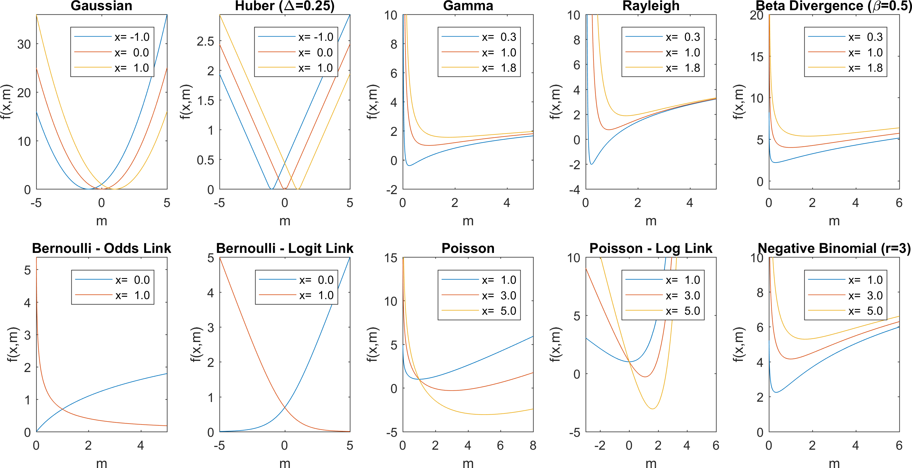
Figure 2: Graphical comparison of different loss functions. Note that some are only defined for binary or integer values of $x$ (bottom row) and that some are only defined for nonnegative values of $x$ and/or $m$.

4 GCP decomposition

We now consider how to compute the GCP for a given elementwise loss function. The majority of this section focuses on dense tensors. Handling sparse or scarce tensors is discussed in Section 4.3.

Recall that we have a data tensor $\bm{\mathscr{{X}}}$ of size $n_{1}\times n_{2}\times\cdots\times n_{d}$ and that $\Omega\subseteq\mathcal{I}$ is the set of indices where the values of $\bm{\mathscr{{X}}}$ are known. For a given $r$, the objective for GCP decomposition is to find the factor matrices ${\bm{\mathbf{{A}}}}_{k}\in\mathbb{R}^{n_{k}\times r}$ for $k=1,\dots,d$ that solve

(25) $$\min\;F(\bm{\mathscr{{M}}};\bm{\mathscr{{X}}},\Omega)\equiv\frac{1}{|\Omega|}\sum_{i\in\Omega}f(x_{i},m_{i})\quad\text{subject to}\quad\bm{\mathscr{{M}}}=\llbracket{\bm{\mathbf{{A}}}}_{1},{\bm{\mathbf{{A}}}}_{2},\dots,{\bm{\mathbf{{A}}}}_{d}\rrbracket.$$

We only sum over the known entries, i.e., $i\in\Omega$; the same approach to missing data has been used for the CP decomposition [3, 4]. We scale by the constant $1/|\Omega|$ so that we are working with the mean. This is simply a convenience that makes it easier to compare function values for tensors with different sizes or different amounts of missing data. This is an optimization problem, and we propose to solve it using an off-the-shelf optimization method, which has been successful for the standard CP decomposition [2, 52] and is amenable to missing data [3, 4]. In contrast to an alternating approach, we do not have to solve a series of optimization problems. The main advantage of the alternating least squares in the solution of the standard CP decomposition is that the subproblems have closed-form solutions [38]; in contrast, the GCP subproblems do not have closed-form solutions so we do not use an alternating method.

We focus on first-order methods, so we need to calculate the gradient of $F$ with respect to the factor matrices. This turns out to have an elegant formulation as shown in Section 4.1. The GCP formulation Eq. 25 can be augmented in various ways. We might add constraints on the factor matrices such as nonnegativity. Another option is to add L2-regularization on the factor matrices to handle the scale ambiguity [2], and we explain how to do this in Section 4.2. We might alternatively want to use L1-regularization on the factor matrices to encourage sparsity. The special structure for sparse and scarce tensors is discussed in Section 4.3.

4.1 GCP gradient

We need the gradient of $F$ in Eq. 25 with respect to the factor matrices, and this is our main result in Theorem 4.4. The importance of this result is that it shows that the gradient can be calculated via a standard tensor operation called the matricized tensor times Khatri-Rao product (MTTKRP), allowing us to take advantage of existing optimized implementations for this key tensor operation. Before we get to that, we establish some useful results in the matrix case. These will be applied to mode-$k$ unfoldings of $\bm{\mathscr{{M}}}$ in the proof of Theorem 4.4. The next result is standard in matrix calculus and left as an exercise for the reader.

Lemma 4.1.

Let ${\bm{\mathbf{{M}}}}={\bm{\mathbf{{A}}}}{\bm{\mathbf{{B}}}}^{\intercal}$ where ${\bm{\mathbf{{A}}}}$ is a matrix of size $n\times r$ and ${\bm{\mathbf{{B}}}}$ is a matrix of size $p\times r$. Then

$$\frac{\partial m_{i\ell}}{\partial a_{i^{\prime}j}}=\begin{cases}b_{\ell j}&\text{if }i=i^{\prime},\\ 0&\text{if }i\neq i^{\prime}\end{cases}\quad\text{for all}\quad i,i^{\prime}\in\set{1,\dots,n},j\in\set{1,\dots,r},\ell\in\set{1,\dots,p}.$$

Next, we consider the problem of generalized matrix factorization in Lemma 4.2, which is our linchpin result. This keeps the index notation simple but captures exactly what we need for the main result in Theorem 4.4. In Lemma 4.2, the matrix ${\bm{\mathbf{{W}}}}$ is an arbitrary matrix of weights for the terms in the summation, and the matrix ${\bm{\mathbf{{Y}}}}$ (which depends on ${\bm{\mathbf{{W}}}}$) is a matrix of derivatives of the elementwise loss function with respect to the model.

Lemma 4.2.

Let ${\bm{\mathbf{{X}}}},{\bm{\mathbf{{W}}}},{\bm{\mathbf{{A}}}},{\bm{\mathbf{{B}}}}$ be matrices of size $n\times p$, $n\times p$, $n\times r$, and $p\times r$, respectively. Let $f:\mathbb{R}\times\mathbb{R}\rightarrow\mathbb{R}$ be a function that is continuously differentiable w.r.t. its second argument. Define the real-valued function $\tilde{F}$ as

(26) $$\tilde{F}({\bm{\mathbf{{M}}}};{\bm{\mathbf{{X}}}},{\bm{\mathbf{{W}}}})=\sum_{i=1}^{n}\sum_{\ell=1}^{p}w_{i\ell}\,f(x_{i\ell},m_{i\ell})\quad\text{subject to}\quad{\bm{\mathbf{{M}}}}={\bm{\mathbf{{A}}}}{\bm{\mathbf{{B}}}}^{\intercal}.$$

Then the first partial derivative of $\tilde{F}$ w.r.t. ${\bm{\mathbf{{A}}}}$ is

$$\frac{\partial\tilde{F}}{\partial{\bm{\mathbf{{A}}}}}={\bm{\mathbf{{Y}}}}{\bm{\mathbf{{B}}}}\quad\in\mathbb{R}^{n\times r}$$

where we define the $n\times p$ matrix ${\bm{\mathbf{{Y}}}}$ as

(27) $$y_{i\ell}=w_{i\ell}\;\frac{\partial f}{\partial m_{i\ell}}(x_{i\ell},m_{i\ell})\quad\text{for all}\quad i\in\set{1,\dots,n},\ell\in\set{1,\dots,p}.$$

Proof 4.3.

Consider the derivative of $\tilde{F}$ with respect to matrix element $a_{ij}$. We have

$$\frac{\partial\tilde{F}}{\partial a_{ij}} =\sum_{i^{\prime}=1}^{n}\sum_{\ell=1}^{p}w_{i^{\prime}\ell}\,\frac{\partial f}{\partial a_{ij}}(x_{i^{\prime}\ell},m_{i^{\prime}\ell}) F$$ by definition of

$$=\sum_{i^{\prime}=1}^{n}\sum_{\ell=1}^{p}w_{i^{\prime}\ell}\,\frac{\partial f}{\partial m_{i^{\prime}\ell}}(x_{i^{\prime}\ell},m_{i^{\prime}\ell})\frac{\partial m_{i^{\prime}\ell}}{\partial a_{ij}} \text{by chain rule},$$

$$=\sum_{\ell=1}^{p}y_{i\ell}b_{\ell j} \text{by \lx@cref{creftype~refnum}{lem:ma} and \lx@cref{creftype~refnum}{eq:Y-mat}}.$$

Rewriting this in matrix notation produces the desired result.

Now we can consider the tensor of the GCP problem Eq. 25 in Theorem 4.4. For simplicity, we replace $\Omega$ with an indicator tensor $\bm{\mathscr{{W}}}$ such that $w_{i}=\delta_{i\in\Omega}$ and rewrite $F$ using $\bm{\mathscr{{W}}}$. Although this result specifies a specific $\bm{\mathscr{{W}}}$, it could be extended to incorporate general weights such as the relative importance of each entry; see Section 6 for further discussion on this topic.

Theorem 4.4 (GCP Gradients).

Let $\bm{\mathscr{{X}}}$ be a tensor of size $n_{1}\times n_{2}\times\cdots\times n_{d}$ and $\Omega$ be the indices of known elements of $\bm{\mathscr{{X}}}$. Let $f:\mathbb{R}\times\mathbb{R}\rightarrow\mathbb{R}$ be a function that is continuously differentiable w.r.t. its second argument. Define $\bm{\mathscr{{W}}}$ to be an indicator tensor such that $w_{i}=\delta_{i\in\Omega}/|\Omega|$. Then we can rewrite the GCP problem Eq. 25 as

(28) $$\min\;F(\bm{\mathscr{{M}}};\bm{\mathscr{{X}}},\bm{\mathscr{{W}}})\equiv\sum_{i\in\mathcal{I}}w_{i}\,f(x_{i},m_{i})\quad\text{subject to}\quad\bm{\mathscr{{M}}}=\llbracket{\bm{\mathbf{{A}}}}_{1},{\bm{\mathbf{{A}}}}_{2},\dots,{\bm{\mathbf{{A}}}}_{d}\rrbracket.$$

Here ${\bm{\mathbf{{A}}}}_{k}$ is a matrix of size $n_{k}\times r$ for $k\in\set{1,\dots,d}$. For each mode $k$, the first partial derivative of $F$ w.r.t. ${\bm{\mathbf{{A}}}}_{k}$ is given by

(29) $$\frac{\partial F}{\partial{\bm{\mathbf{{A}}}}_{k}missing}={\bm{\mathbf{{Y}}}}_{(k)}{\bm{\mathbf{{Z}}}}_{k}$$

where ${\bm{\mathbf{{Z}}}}_{k}$ is defined in Eq. 7 and ${\bm{\mathbf{{Y}}}}_{(k)}$ is the mode-$k$ unfolding of a tensor $\bm{\mathscr{{Y}}}$ defined by

(30) $$y_{i}=w_{i}\,\frac{\partial f}{\partial m_{i}missing}(x_{i},m_{i})\quad\text{for all}\quad i\in\mathcal{I}.$$

Proof 4.5.

For a given $k$, recall that ${\bm{\mathbf{{M}}}}_{(k)}={\bm{\mathbf{{A}}}}_{k}{\bm{\mathbf{{Z}}}}_{k}^{\intercal}$. Hence, we can write $F$ in Eq. 28 as

$$F(\bm{\mathscr{{M}}};\bm{\mathscr{{X}}},\bm{\mathscr{{W}}})=\tilde{F}({\bm{\mathbf{{A}}}}_{k}^{\phantom{\intercal}}{\bm{\mathbf{{Z}}}}_{k}^{\intercal};{\bm{\mathbf{{X}}}}_{(k)},{\bm{\mathbf{{W}}}}_{(k)}),$$

where $\tilde{F}$ is from Eq. 26. The result follows from Lemma 4.2 with the substitutions used in the following table:

Matrix Case	${\bm{\mathbf{{X}}}}$	${\bm{\mathbf{{W}}}}$	${\bm{\mathbf{{A}}}}$	${\bm{\mathbf{{B}}}}$	${\bm{\mathbf{{Y}}}}$	$n$	$p$	$r$
Tensor Case	${\bm{\mathbf{{X}}}}_{(k)}$	${\bm{\mathbf{{W}}}}_{(k)}$	${\bm{\mathbf{{A}}}}_{k}$	${\bm{\mathbf{{Z}}}}_{k}$	${\bm{\mathbf{{Y}}}}_{(k)}$	$n_{k}$	$n^{d}/n_{k}$	$r$

We note that the definition of $\bm{\mathscr{{Y}}}$ is consistent across all $k$.

Theorem 4.4 generalizes several previous results: the gradient for CP [55, 2], the gradient for CP in the case of missing data [4], and the gradient for Poisson tensor factorization [16].

Consider the gradient in Eq. 29. The ${\bm{\mathbf{{Z}}}}_{k}$ has no dependence on $\bm{\mathscr{{X}}}$, $\Omega$, or the loss function; it depends only on the structure of the model. Conversely, $\bm{\mathscr{{Y}}}$ has no dependence on the structure of the model. The elementwise derivative tensor $\bm{\mathscr{{Y}}}$ is the same size as $\bm{\mathscr{{X}}}$ and is zero wherever $\bm{\mathscr{{X}}}$ is missing data. The structure of $\Omega$ determines the structural sparsity of $\bm{\mathscr{{Y}}}$, and this will be important in Section 4.3. The form of the derivative is a matricized tensor times Khatri-Rao product (MTTKRP) with the tensor $\bm{\mathscr{{Y}}}$ and the Khatri-Rao product ${\bm{\mathbf{{Z}}}}_{k}$. The MTTKRP is the dominant kernel in the standard CP computation in terms of computation time and has optimized high-performance implementations [7, 56, 40, 31]. In the dense case, the MTTKRP costs $\mathcal{O}(rn^{d})$.

Algorithm 1 computes the GCP loss function and gradient. On 2 we compute elementwise values at known data locations. If all or most elements are known, we can compute the full model using Eq. 7 at a cost of $rn^{d}$. However, if only a few elements are known, it may be more efficient to compute model values only at the locations in $\Omega$ using Eq. 6 at a cost of $2r|\Omega|$. We compute the elementwise derivative tensor $\bm{\mathscr{{Y}}}$ in 4; here the quantity $\delta_{i\in\Omega}$ is 1 if $i\in\Omega$ and 0 otherwise. The cost of 3 and 4 is $O(|\Omega|)$. 5, 6 and 7 compute the gradient with respect to each factor matrix, and the cost is $O(drn^{d})$. Communication lower bounds as well as a parallel implementation for MTTKRP for dense tensors are covered in [9]. Since this is a sequence of MTTKRP operations, we can also consider reusing intermediate computations as has been done [51] and reduces the $d$ part of the expense. Hence, the cost is dominated by the MTTKRP, just as for the standard CP-ALS. We revisit this method in the case of sparse or large-scale tensors in Section 4.3.

Algorithm 1 GCP loss function and gradient

1:function gcp_fg($\bm{\mathscr{{X}}}$,$\Omega$,$\set{{\bm{\mathbf{{A}}}}_{k}missing}{k=1,\dots,d}$)

2:      $m_{i}\leftarrow\textsc{entry}(\set{{\bm{\mathbf{{A}}}}_{k}missing}{k=1,\dots,d},i)$ for all $i\in\Omega$ $\triangleright$ Model entries

3:      $F\leftarrow\frac{1}{|\Omega|}\sum_{i\in\Omega}f(x_{i},m_{i})$ $\triangleright$ Loss function

4:      $y_{i}\leftarrow(\delta_{i\in\Omega}/|\Omega|)\,\frac{\partial f}{\partial m_{i}missing}(x_{i},m_{i})$ for all $i\in\mathcal{I}$ $\triangleright$ Elementwise derivative tensor

5:     for $k=1,\dots,d$ do $\triangleright$ Full sequence of MTTKRPs

6:          ${\bm{\mathbf{{G}}}}_{k}\leftarrow\textsc{mttkrp}(\bm{\mathscr{{Y}}},\llbracket{\bm{\mathbf{{A}}}}_{1},{\bm{\mathbf{{A}}}}_{2},\dots,{\bm{\mathbf{{A}}}}_{d}\rrbracket,k)$ $\triangleright$ Gradients w.r.t. ${\bm{\mathbf{{A}}}}_{k}$

7:     end for

8:     return $F$ and $\set{{\bm{\mathbf{{G}}}}_{k}missing}{k=1,\dots,d}$

9:end function

4.2 Regularization

It is straightforward to add regularization to the GCP formulation. This may especially be merited when there is a large proportion of missing data, in which case some of the factor elements may not be constrained due to lack of data. As an example, consider simple L2 regularization. We modify the GCP problem in Eq. 25 to be

(31) $$\min F(\bm{\mathscr{{M}}};\bm{\mathscr{{X}}},\Omega,\set{\eta_{k}})\equiv\frac{1}{|\Omega|}\sum_{i\in\Omega}f(x_{i},m_{i})+\sum_{k=1}^{d}\frac{\eta_{k}}{2}\|{\bm{\mathbf{{A}}}}_{k}\|_{2}^{2}\\ \quad\text{subject to}\quad\bm{\mathscr{{M}}}=\llbracket{\bm{\mathbf{{A}}}}_{1},{\bm{\mathbf{{A}}}}_{2},\dots,{\bm{\mathbf{{A}}}}_{d}\rrbracket.$$

In this case, the gradients are given by

(32) $$\frac{\partial F}{\partial{\bm{\mathbf{{A}}}}_{k}missing}={\bm{\mathbf{{Y}}}}_{(k)}{\bm{\mathbf{{Z}}}}_{k}+\eta_{k}{\bm{\mathbf{{A}}}}_{k},$$

where ${\bm{\mathbf{{Y}}}}_{(k)}$ and ${\bm{\mathbf{{Z}}}}_{k}$ are the same as in Eq. 30. The difficulty is in picking the regularization parameters, $\set{\eta_{k}}$. These can all be equal or different, and can be selected by cross-validation using prediction of held out elements.

4.3 GCP Decomposition for Sparse or Scarce Tensors

We say a tensor is sparse if the vast majority of its entries are zero. In contrast, we say a tensor is scarce if the vast majority of its entries are missing. In either case, we can store such a tensor efficiently by keeping only its nonzero/known values and the corresponding indices. If $s$ is the number of nonzero/known values, the required storage is $s(d+1)$ rather than $n^{d}$ for the dense tensor where every zero or unknown value is stored explicitly.

The fact that $\bm{\mathscr{{X}}}$ is sparse does not imply that the $\bm{\mathscr{{Y}}}$ tensor needed to compute the gradient (see Theorem 4.4) is sparse. This is because $\frac{\partial f}{\partial m_{i}missing}(0,m_{i})\neq 0$ for general values of $m_{i}$. There are two cases where the gradient has a structure that allows us to avoid explicitly calculating $\bm{\mathscr{{Y}}}$:

• Standard Gaussian formulation; see Appendix B for details.

• Poisson formulation with the identity link; see [16] for details.

Otherwise, we have to calculate the dense $\bm{\mathscr{{Y}}}$ explicitly in order to compute the gradients. For many large-scale tensors, this is infeasible. The fact that $\bm{\mathscr{{X}}}$ is scarce, however, does imply that the tensor $\bm{\mathscr{{Y}}}$ is sparse. This is because all missing elements in $\bm{\mathscr{{X}}}$ correspond to zeros in $\bm{\mathscr{{Y}}}$.

Let us take a moment to contrast the implication of sparse versus scarce. Recall that a sparse tensor is one where the vast majority of elements are zero, whereas a scarce tensor is one where the vast majority of elements are missing. The elementwise gradient tensor $\bm{\mathscr{{Y}}}$ for a sparse tensor is structurally dense, but it is sparse for a scarce tensor. To put it another way, if $\bm{\mathscr{{X}}}$ is sparse, then the MTTKRP calculation in 6 of Algorithm 1 has a dense $\bm{\mathscr{{Y}}}$; but if $\bm{\mathscr{{X}}}$ is scarce, then the MTTKRP calculation uses a sparse $\bm{\mathscr{{Y}}}$. Further discussion of sparse versus scarce in the matrix case can be found in a blog post by Kolda [37]. We summarize the situation in Fig. 3.

$\displaystyle\text{Dense }\bm{\mathscr{{X}}}$ $\displaystyle\Rightarrow\text{Dense }\bm{\mathscr{{Y}}}$ $\displaystyle\text{Sparse }\bm{\mathscr{{X}}}$ $\displaystyle\Rightarrow\text{Dense }\bm{\mathscr{{Y}}}$ $\displaystyle\text{Scarce }\bm{\mathscr{{X}}}$ $\displaystyle\Rightarrow\text{Sparse }\bm{\mathscr{{Y}}}$

Figure 3: Contrasting sparsity and scarcity in GCP.

The idea that scarcity yields sparsity in the gradient calculation suggests several possible approaches for handling large-scale tensors. One possibility is to simply leave out some of the data, i.e., impose scarcity. Consider that we have a vastly overdetermined problem because we have $n^{d}$ observations but only need to determine $rd\bar{n}$ parameters. Special care needs to be taken if the tensor is sparse, since leaving out the vast majority of the nonzero entries would clearly degrade the solution. Another option is to consider stochastic gradient descent, where the batch at each iteration can be considered as a scarce tensor, leading again to a sparse $\bm{\mathscr{{Y}}}$ in the gradient calculation. These are topics that we will investigate in detail in future work.

5 Experimental results

The goal of GCP is to give data analysts the flexibility to try out different loss functions. In this section, we show examples that illustrate the differences in the tensor factorization from using different loss functions. We do not claim that any particular loss function is better than any other; instead, we want to highlight the ability to easily use different loss functions. Along the way, we also show the general utility of tensor decomposition, which includes:

• Data decomposition into explanatory factors: We can directly visualize the resulting components and oftentimes use this for interpretation. This is analogous to matrix decompositions such as principal component analysis, independent component analysis, nonnegative matrix factorization, etc.

• Compressed object representations: Object $i_{k}$ in mode $k$ corresponds to row $i_{k}$ in factor matrix ${\bm{\mathbf{{A}}}}_{k}$, which is a length-$r$ vector. This can be used as input to regression, clustering, visualization, machine learning, etc.

We focus primarily on these types of activities. However, we could also consider filling in missing data, data compression, etc.

All experiments are conducted in MATLAB. The method is implemented as gcp_opt in the Tensor Toolbox for MATLAB [8, 6]. For the optimization, we use limited-memory BFGS with bound constraints (L-BFGS-B) [14]. First-order optimization methods such as L-BFGS-B typically expect a vector-valued function $f:\mathbb{R}^{n}\rightarrow\mathbb{R}$ and a corresponding vector-valued gradient, but the optimization variables in GCP are matrix-valued; see Appendix C for discussion of how we practically handle the required reshaping. For simplicity, we choose a rank that works reasonably well for the purposes of illustration. Generally, however, the choice of model rank is a complex procedure. It might be selected based on model consistency across multiple runs, cross-validation for estimation of hold-out data, or some prediction task using the factors. Likewise, we choose an arbitrary “run” for the purposes of illustration. These are nonconvex optimization problems, and so we are not guaranteed that every run will find the global minimum. In practice, a user would do a few runs and usually choose the one with the lowest objective value.

5.1 Social network

We consider the application of GCP to a social network dataset. Specifically, we use a chat network from students at UC Irvine [44, 49, 45]. It contains transmission times and sizes of 59,835 messages sent among 1899 anonymized users over 195 days from April to October 2004. Because many of the users included in the dataset sent few messages, we select only the 200 most prolific senders in this analysis. We consider a three-way binary tensor of size $200\times 200\times 195$ of the following form:

$$x(i_{1},i_{2},i_{3})=\begin{cases}1&\text{if student $i_{1}$ sent a message to student $i_{2}$ on day $i_{3}$,}\\ 0&\text{otherwise}.\end{cases}$$

It has 9764 nonzeros, so it is only 0.13% dense though we treat it as dense in this work. The number of interacting pairs per day is shown in Fig. 4a, and there is clearly more activity earlier in the study. To give a sense of how many days any given pair of students interact, we consider the histogram in Fig. 4b. The vast majority of students that interacted had only one interaction, i.e., $4\times 10^{4}$ of the interactions were for only one day. The maximum number of interaction days was 33, which occurred for only one pair.

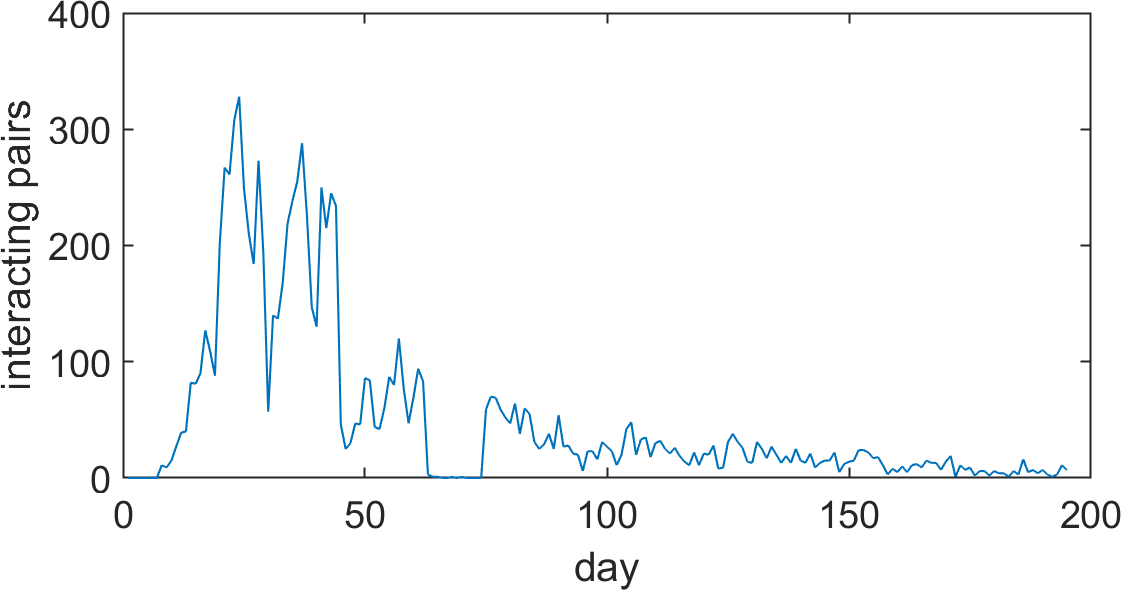
(a) Number of interacting pairs per day. Note the gap around day 70 and the decrease in activity toward the end of the experiment.

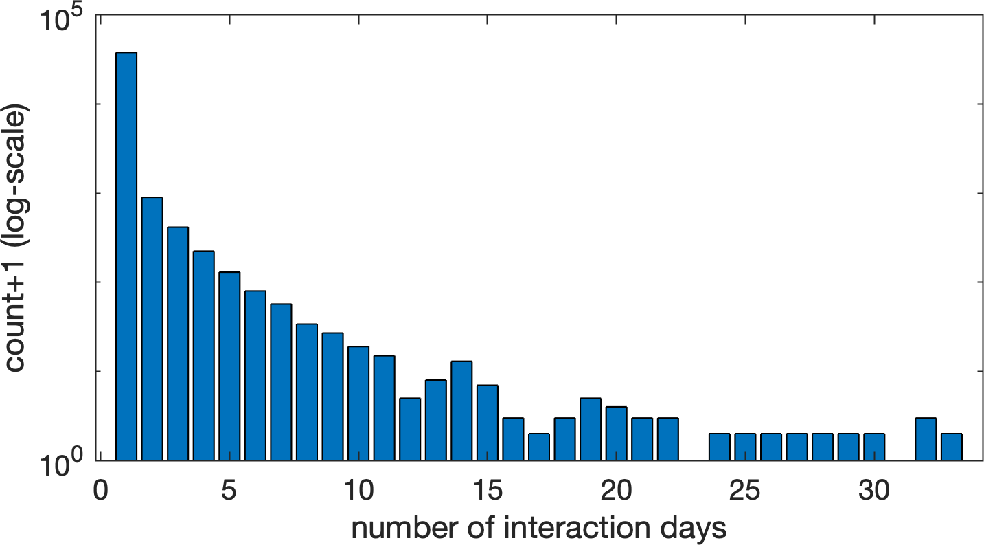
(b) Histogram of number of interactions per pair where count is in the log scale. Most students only interact once. The greatest number of interaction days is 33.

Figure 4: Statistics for a social network tensor where $x(i_{1},i_{2},i_{3})=1$ if student $i_{1}$ sends a message to student $i_{2}$ on day $i_{3}$.

5.1.1 Explanatory factors for social network

We compare the explanatory GCP factors using three different loss functions in Fig. 5. Recall that each component is the outer product of three vectors; these vectors are what we plot to visualize the model. In all cases, we use $r=7$ components because it seemed to be adequately descriptive. To visualize the factorization, components are shown as “rows”, numbered on the left, and ordered by magnitude. We show all three modes as bar plots. The first two modes correspond to students, as senders and receivers. They are ordered from greatest to least total activity and normalized to unit length. The third mode is day, and it is normalized to the magnitude of the component. Each component groups students that are messaging one another along with the dates of activity. Each loss function yields a different grouping and so a different interpretation. The appropriateness of any particular interpretation depends on the context.

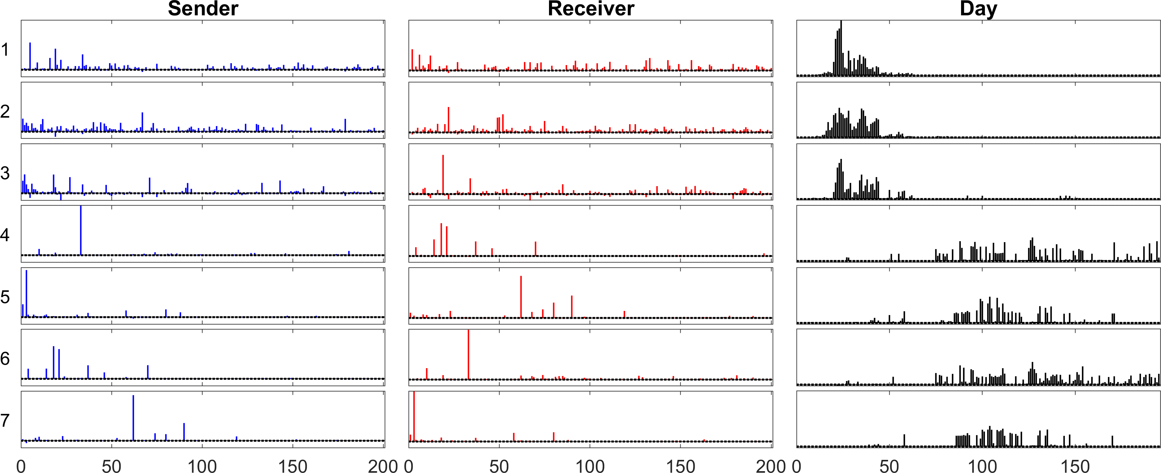
(a) Gaussian (standard CP). Some factors only pick up one or two students as senders or receivers.

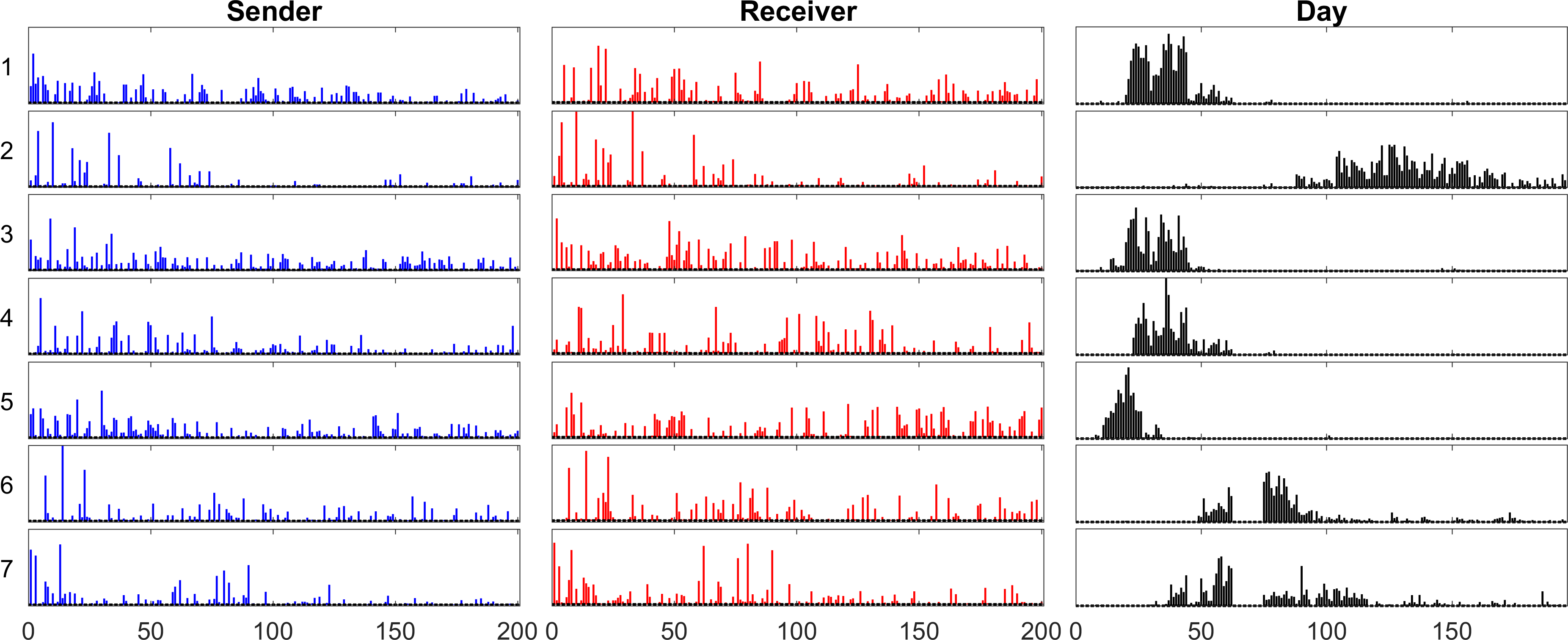
(b) Bernoulli-odds (with nonnegativity constraints). Compared with CP-ALS, many students are identified with each component and more emphasis is placed on the heavier traffic days.

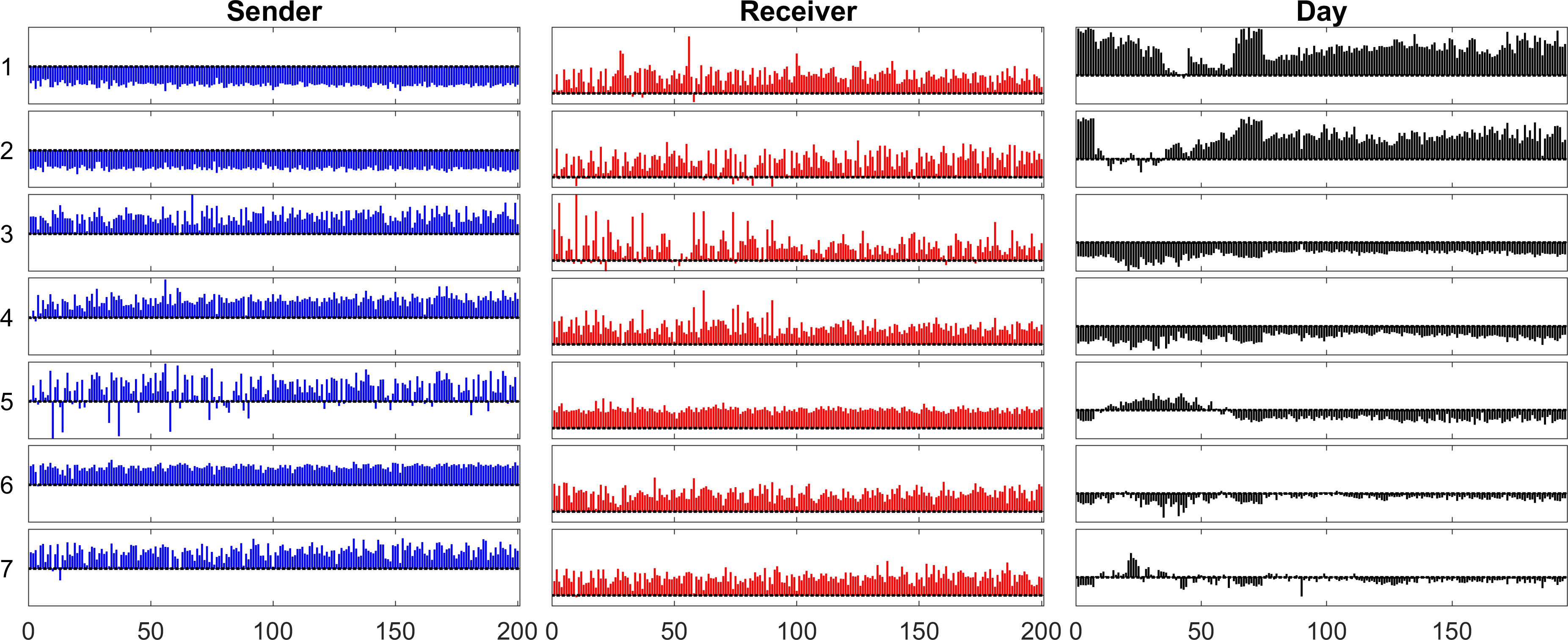
(c) Bernoulli-logit. A negative product means the likely result is a zero, i.e., no communication. The first few factors are focused primarily on the zeros.

Figure 5: GCP tensor decomposition of $200\times 200\times 195$ binary (0/1) social network tensor using different loss functions and $r=7$.

For the standard CP in Fig. 5a, we did not add a nonnegative constraint on the factors, but there are only a few small negative entries (see, e.g., the third component). There is a clear temporal locality in the first three factors. The remaining four are more diffuse. A few sender/receiver factors capture only a few large magnitude entries: sender factor 4, receiver factor 6, and both sender/receiver factors 7.

For Bernoulli with an odds link in Fig. 5b, the factor matrices are constrained to be nonnegative. We see even more defined temporal locality in this version. In particular, components 6 and 7 do not really have an analogue in the Gaussian version. The sender and receiver factors are correlated with one another in components 2, 6, and 7, which is something that we did not really see in the Gaussian case. Such correlations are indicative of a group talking to itself. The factors in this case seem to do a better job capturing the activity on the most active days per Fig. 4a.

For Bernoulli with a logit link in Fig. 5c, the interpretation is very different. Recall that negative values correspond to observing zeros. The first component is roughly inversely correlated with the activity per day, i.e., most entries are zeros and this is what is picked up. It is only really in components 5 and 7 where there is some push toward positive values, i.e., interactions.

5.1.2 Prediction for social network

To show the benefit of using a different loss function, we consider the problem of predicting missing values. We run the same experiment as before but hold out 50 ones and 50 zeros at random when fitting the model. We then use the model to predict the held out values. Let $\Omega$ denote the set of known values, so $i\not\in\Omega$ means that the entry was held out. We measure the accuracy of the prediction using the log-likelihood under a Bernoulli assumption, i.e., we compute

$$\text{log-likelihood}=\sum_{{x_{i}=1}\atop{i\not\in\Omega}}\log p_{i}+\sum_{{x_{i}=0}\atop{i\not\in\Omega}}\log(1-p_{i}),$$

where $p_{i}$ is the probability of a one as predicted by the model. A higher log-likelihood indicates a more accurate prediction. We convert the predicted values $m_{i}$, computed from Eq. 6, to probabilities $p_{i}$ (truncated to the range $[10^{-16},1-10^{-16}]$) as follows:

• Gaussian. Let $p_{i}=m_{i}$, truncating to the range (0,1).

• Bernoulli-odds. Convert from the odds ratio: $p_{i}=m_{i}/(1+m_{i})$.

• Bernoulli-logit. Convert from the log-odds ratio: $p_{i}=e^{m_{i}}/(1+e^{m_{i}})$.

We repeat the experiment two hundred times, each time holding out a different set of 100 entries. The results are shown in Fig. 6. This is a difficult prediction problem since ones are extremely rare; the differences in prediction performance were negligible for predicting the zeros but predicting the ones was much more difficult. Both Bernoulli-odds and Bernoulli-logit consistently outperform the standard approach based on a Gaussian loss function. We also note that the Gaussian-based predictions were outside of the range $[0,1]$ for 11% of the predictions, making it tricky to interpret the Gaussian-based predictions.

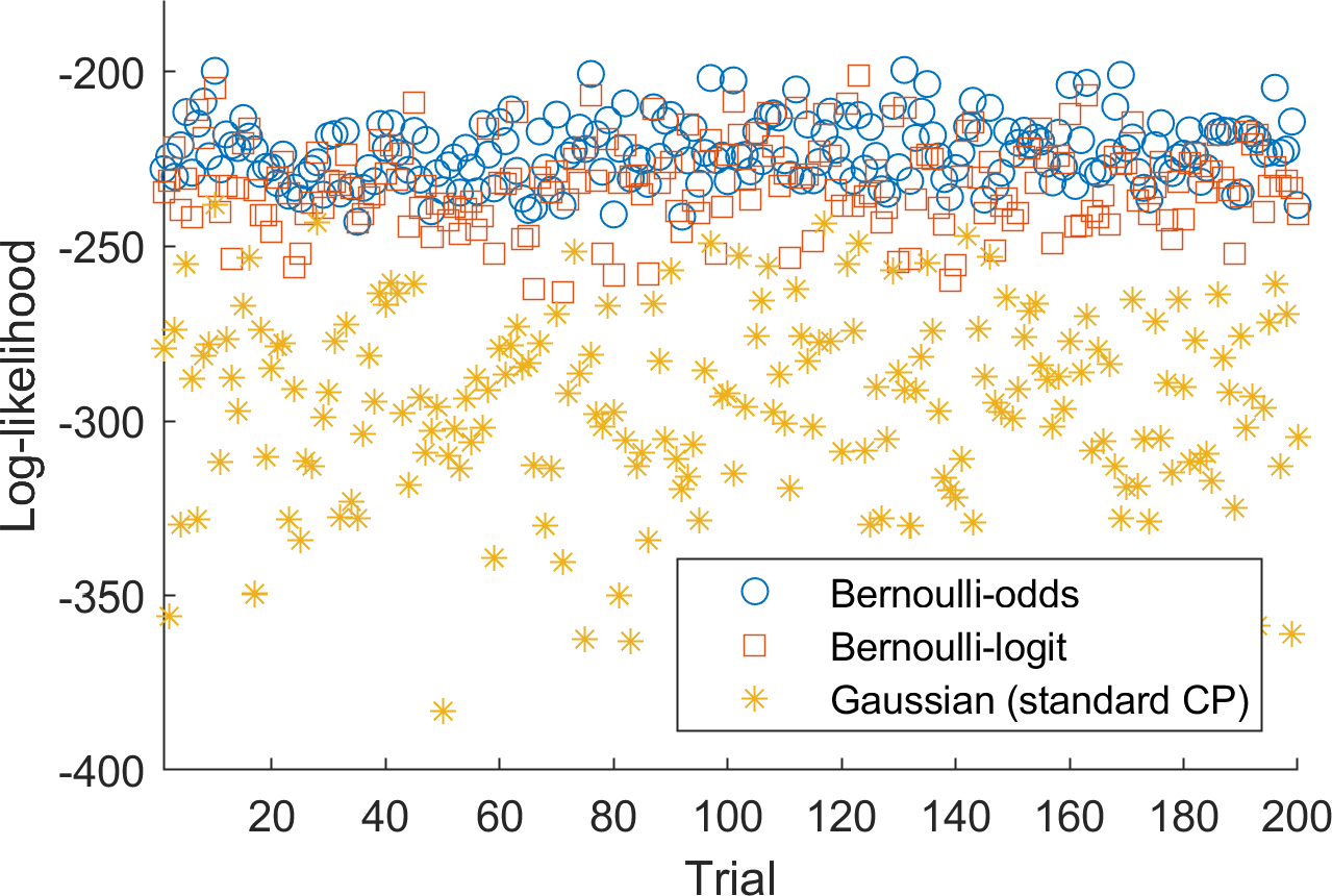
(a) Prediction of 100 missing entries for 200 trials.

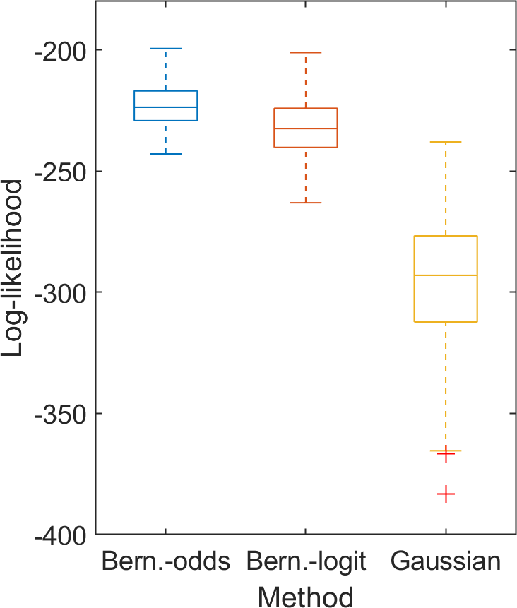
(b) Box plot of prediction results.

Figure 6: Log-likelihood for GCP with different loss functions. Each trial holds out 50 ones and 50 zeros at random. The GCPs are computed and used to estimate each held-out value. A higher log-likelihood indicates a better prediction. In the box plot, the box represents 25th–75th percentiles with a horizontal midline at the 50th percentile, i.e., the median. The whiskers extend to the most extreme data points that are not considered outliers, and then outliers are indicated with plus-symbols.

5.2 Neural activity of a mouse

In recent work, Williams et al. [60] consider the application of CP tensor decomposition to analyze the neural activity of a mouse completing a series of trials. They have provided us with a reduced version of their dataset to illustrate the utility of the GCP framework. In the dataset we study, the setup is as follows. A mouse runs a maze over and over again, for a total of 300 trials. The maze has only one junction, at which point the mouse must turn either right or left. The mouse is forced to learn which way to turn in order to receive a reward. For the first 75 trials, the mouse gets a reward if it turns right; for the next 125 trials, it gets a reward if it turns left; and for the final 100 trials, it gets a reward if it turns right. Data was recorded from the prefrontal cortex of a mouse using calcium imaging; specifically, the activity of 282 neurons was recorded and processed so that all data values lie between 0 and 1. The neural activity in time for a few sample neurons is shown in Fig. 7; we plot each of the 300 different trials and the average value. From this image, we can see that different neurons have distinctive patterns of activity. Additionally, we see an example of at least one neuron that is clearly active for some trials and not for others (Neuron 117).

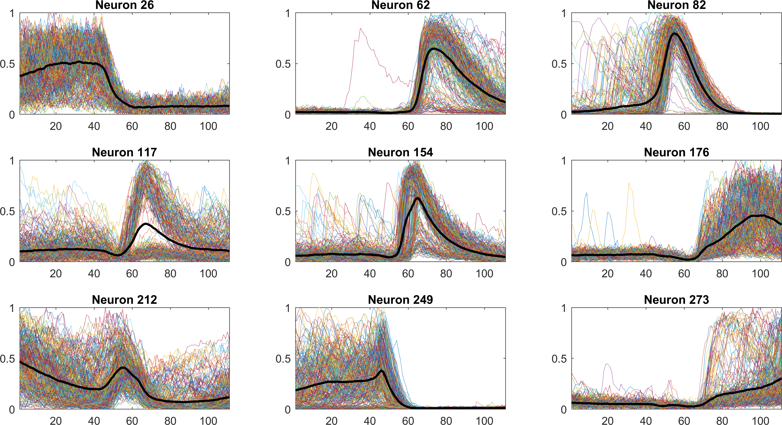
Figure 7: Example neuron activity across all trials. Each thin line (randomly colored) is the time profile for a single trial, and the single dark line is the average over all 300 trials. Different neurons have distinctive temporal patterns. Moreover, some have markedly different activity for different trials, like Neuron 117.

This is large and complex multiway data. We can arrange this data as a three-way nonnegative tensor as follows: 282 (neurons) $\times$ 110 (time points) $\times$ 300 trials. Applying GCP tensor decomposition reduces the data into explanatory factors, as we discuss in Section 5.2.1. We show how the factors can be used in a regression task in Section 5.2.2.

5.2.1 Explanatory factors for mouse neural activity

We compare the results of using different loss functions in terms of explanatory factors. In all cases, we use $r=8$ components. The first mode corresponds to the neurons and is normalized to the size of the component, The second and third modes are, respectively, within-trial time and trial, each normalized to length 1. The neuron factors are plotted as bar graphs, showing the activation level of each neuron. We emphasize in red the bars that correspond to the example neurons from Fig. 7. The time factors are plotted as lines, and turn out to be continuous because that is an inherent feature of the data itself. We did nothing to enforce continuity in those factors. The trial factors are scatter plots, color coded to indicate which way the mouse turned. The dot is filled in if the mouse received a reward. When the rules changed (at trial 75 and 200, indicated by vertical dotted lines), the mouse took several trials to figure out the new way to turn for the reward.

The result of a standard CP analysis is shown in Fig. 8a. Several components are strongly correlated with the trial conditions, indicating the power of the CP analysis. For instance, component 3 correlates with receiving a reward (filled). Components 5, 6, and 8 correlate to turning left (orange) and right (green). Their time profiles align with when these activities are happening (e.g., end of trial for reward and mid-trial for turn). The problem with the standard CP model is that interpretation of the negative values is difficult. Consider that neuron 212 has a significant score for nearly every component, making it hard to understand its role. Indeed, several of the example neurons have high magnitude scores for multiple components, and so it might be hard to hypothesize which neurons correspond to which trial conditions.

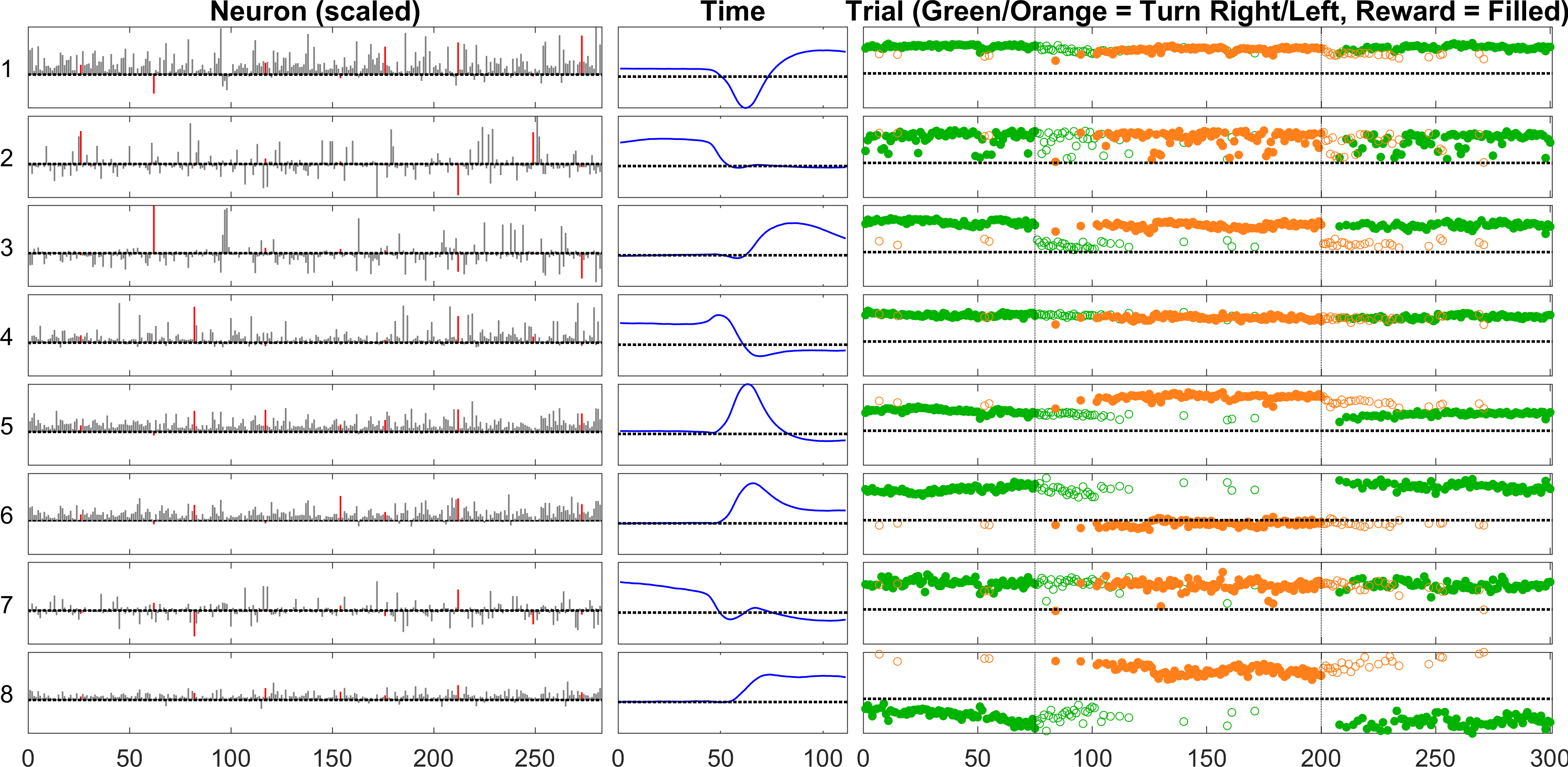
(a) Gaussian (standard CP) is difficult to interpret because of negative values

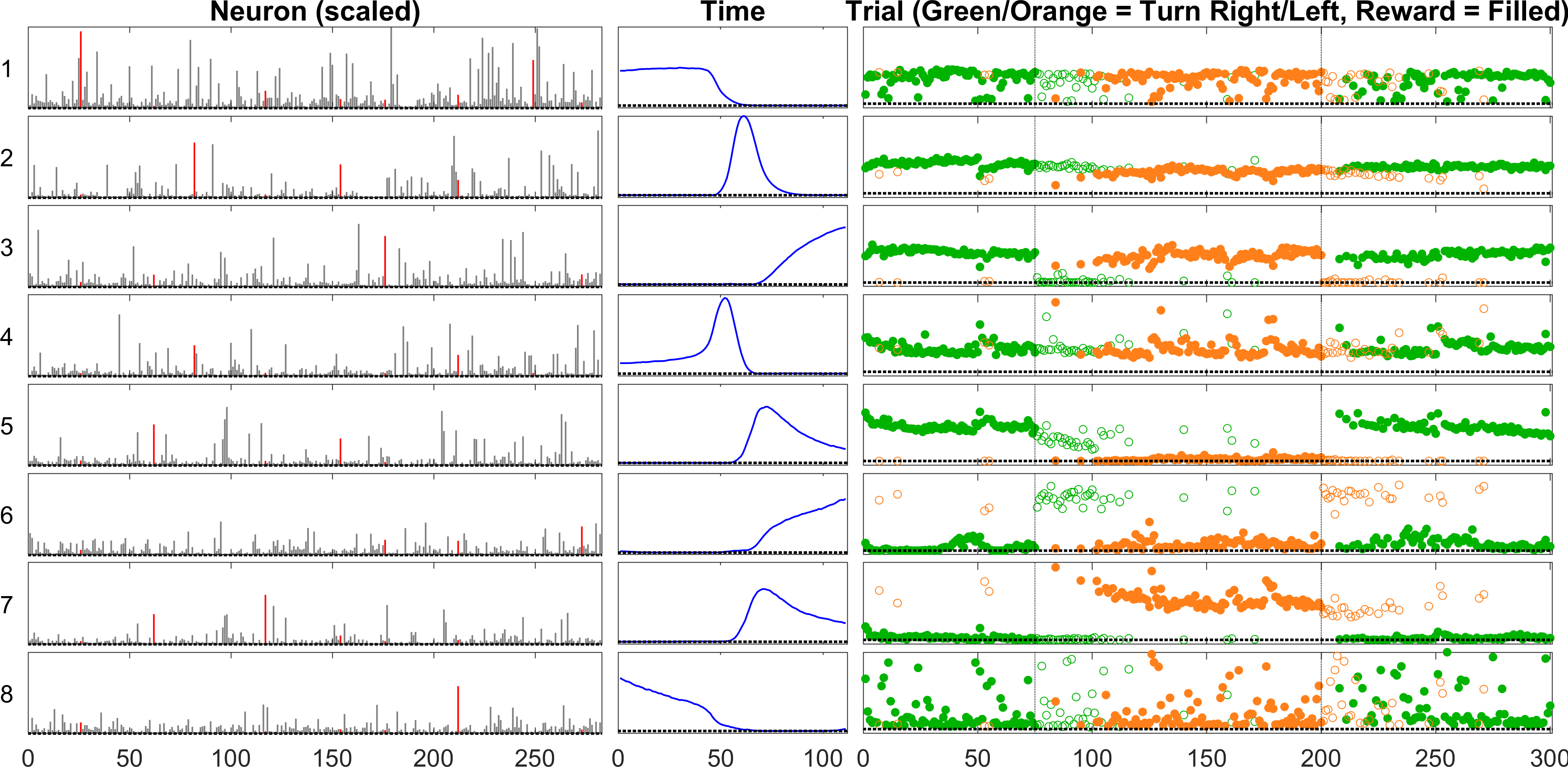
(b) Beta-divergence with $\beta{=}0.5$ has no negative factor values and so is easier to interpret

Figure 8: GCP tensor decomposition of mouse neural activity. Components ordered by size (top to bottom). Example neurons (26, 62, 82, 117, 154, 176, 212, 249, 273) highlighted in red. Trial symbols are coded by conditions: color indicates turn and filled indicates a reward. The rule changes are denoted by vertical dotted lines. Observe that some factors split the trials by turn (green versus orange) and others split by reward (open versus filled), even though the tensor decomposition has no knowledge of the trial conditions.

In contrast, consider Fig. 8b which shows the results of GCP with $\beta$-divergence with $\beta=0.5$. The factorization is arguably easier to interpret since it has only nonnegative values. As before, we see that several components clearly correlate with the trial conditions. Components 3 and 6 correlate with reward conditions. Components 5 and 7 correlate to the turns. In this case, the example neurons seem to have clearer identities with the factors. Neuron 176 is strongest for factor 3 (reward), whereas neuron 273 is strongest for factor 6 (no reward). Some of the components do not correspond to the reward or turn, and we do not always know how to interpret them. They may have to do with external factors that are not recorded in the experimental metadata. We might also hypothesize interpretations for some components. For instance, the second component is active mid-trial and may have to do with detecting the junction in the maze.

For further comparison, we include the results of using Rayleigh, Gamma, and Huber loss functions in Fig. 9. These capture many of the same trends.

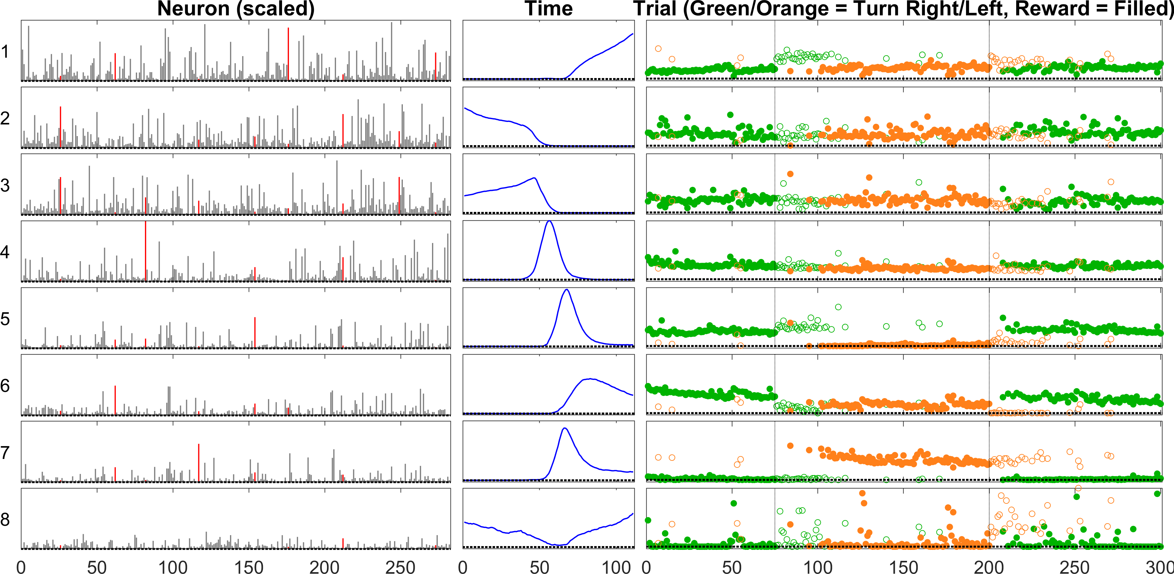
(a) Rayleigh with nonnegativity constraints

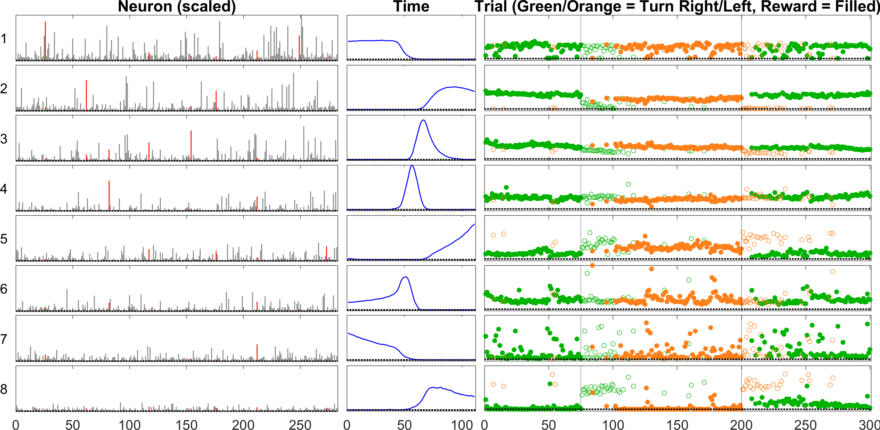
(b) Gamma with nonnegativity constraints

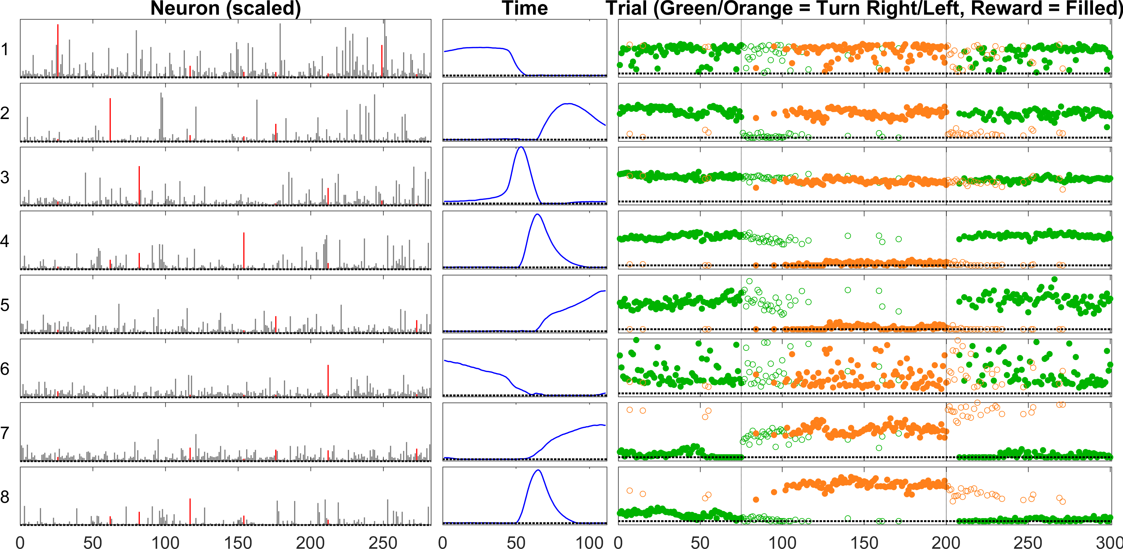
(c) Huber with $\Delta{=}0.25$ and nonnegativity constraints

Figure 9: Additional GCP tensor decompositions of mouse neural activity.

5.2.2 Regression task for mouse neural activity

Recall that the tensor factorization has no knowledge of the experimental conditions, i.e., which way the mouse turned or whether or not it received a reward. Suppose that the experimental logs were corrupted in such a way that we lost 50% of the trial indicators (completely at random rather than in a sequence). For instance, we might not know whether the mouse turned left or right in Trial 87. We can use the results of the GCP tensor factorization to recover that information. Observe that each trial is represented by 8 values, i.e., a score for each component. These vectors can be used for regression.

Our experimental setup is as follows. We randomly selected 50% of the 300 trials as training data and use the remainder for testing. We do simple linear regression. Specifically, we let ${\bm{\mathbf{{A}}}}_{3}^{\rm train}$ be the rows of ${\bm{\mathbf{{A}}}}_{3}$ corresponding to the training trials and $\mathbf{y}^{\rm train}$ be the corresponding binary responses (e.g., 1 for left turn and 0 for right turn). We solve the regression problem:

$$\min_{{\bm{\mathbf{{\beta}}}}}\|{\bm{\mathbf{{A}}}}_{3}^{\rm train}{\bm{\mathbf{{\beta}}}}-\mathbf{y}^{\rm train}\|.$$

We let ${\bm{\mathbf{{A}}}}_{3}^{\rm test}$ be the rows of ${\bm{\mathbf{{A}}}}_{3}$ corresponding to the testing trials. Using the optimal ${\bm{\mathbf{{\beta}}}}$, we make predictions for $\mathbf{y}^{\rm test}$ by computing

$${\bm{\hat{\mathbf{{y}}}}}^{\rm test}=\left[{\bm{\mathbf{{A}}}}_{3}^{\rm test}{\bm{\mathbf{{\beta}}}}\geq 0.5\right].$$

We did this 100 times, both for determining the turn direction (left or right) and the reward (yes or no).

The results are shown in Table 2. We caution that these are merely for illustrative purposes as changing the ranks and other parameters might impact the relative performance of the methods. For the turn results, shown in Table 2a, only the Gamma loss failed to achieve perfect classification. We can see which factors were most important based on the regression coefficients. For instance, the sixth component is clearly the most important for Gaussian, whereas the fifth and seventh are key for $\beta$-divergence. The reward was harder to predict, per the results in Table 2b. This is likely due to the fact that there were relatively few times when the reward was not received. For instance, the Rayleigh method performed worst, in contrast to its perfect classification for the turn direction. Only the $\beta$-divergence achieved perfect regression with the third component being the most important predictor.

Loss	Regression Coefficients								Max	Incorrect
Type	1	2	3	4	5	6	7	8	Std. Dev.	out of 15000
Gaussian	-9.6	2.1	0.5	-0.8	3.7	15.9	3.5	1.3	2.2e+00	0
Beta Div.	5.5	5.4	-4.6	3.0	5.9	-1.8	-5.6	1.9	1.2e+00	0
Rayleigh	2.7	1.9	1.2	0.9	5.6	3.7	-5.3	-0.4	1.2e+00	0
Gamma	-15.1	22.4	6.2	4.3	-0.3	-7.6	-8.2	10.5	3.0e+00	1454
Huber	2.8	-1.3	3.4	9.7	-0.6	1.4	-1.5	-2.7	7.1e-01	0

(a) Turn

Loss	Regression Coefficients								Max	Incorrect
Type	1	2	3	4	5	6	7	8	Std. Dev.	out of 15000
Gaussian	11.6	-0.5	18.7	-2.1	-6.9	-8.6	0.0	-3.2	3.6e+00	37
Beta Div.	5.1	-0.8	7.4	-0.1	2.8	-3.8	2.6	2.4	1.1e+00	0
Rayleigh	-6.3	8.5	8.1	1.0	-1.6	5.1	1.9	-3.0	1.3e+00	520
Gamma	10.7	1.9	0.5	0.3	-2.1	3.6	5.6	-6.4	1.3e+00	172
Huber	3.0	13.5	-9.0	2.3	2.5	2.2	-1.0	4.0	1.3e+00	62

(b) Reward

Table 2: Regression coefficients and prediction performance for different loss functions

5.3 Rainfall in India

We consider monthly rainfall data for different regions in India for the period 1901–2015, available from Kaggle. For each of 36 regions, 12 months, and 115 years, we have the total rainfall in millimeters. There is a small amount of missing data (0.72%), which GCP handles explicitly. We show example monthly rainfalls for 6 regions in Fig. 10.

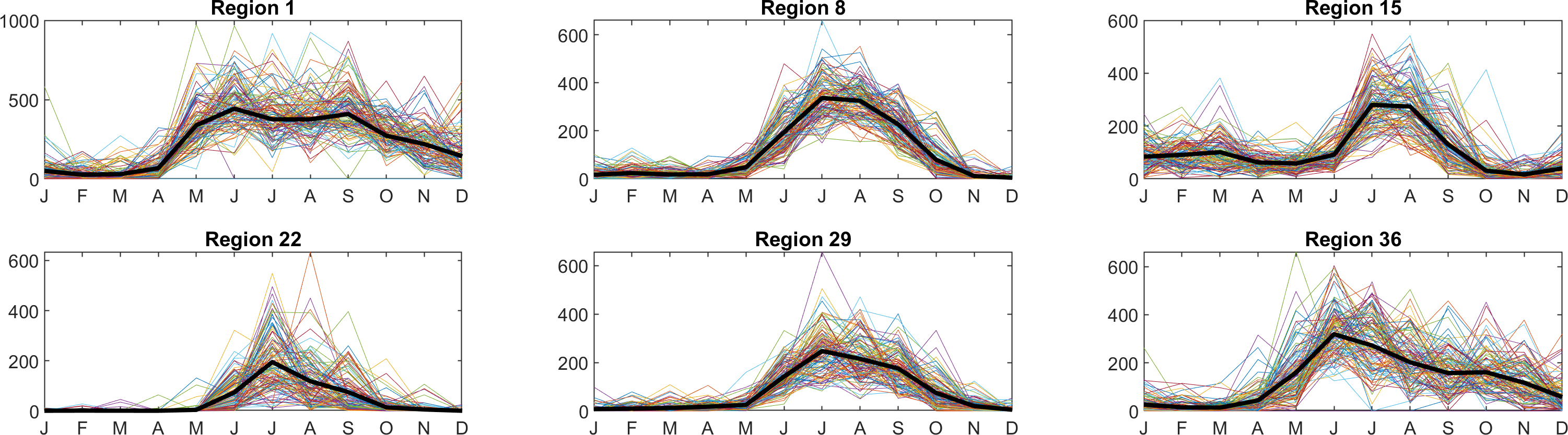
Figure 10: Rainfall totals per month in several regions in India. Each colored thin line represents a single year. The average is shown as a thick black line. Monsoon season is June – September.

Oftentimes the gamma distribution is used to model rainfall. A histogram of all monthly values is shown in Fig. 11 along with the estimated gamma distribution (in red), and it seems as though a gamma distribution is potentially a reasonable model. Most rainfall totals are very small (the smallest nonzero value is 0.1mm, which is presumably the precision of the measurements), but the largest rainfall in a month exceeds 2300mm. For this reason, we consider the GCP tensor decomposition with gamma loss.

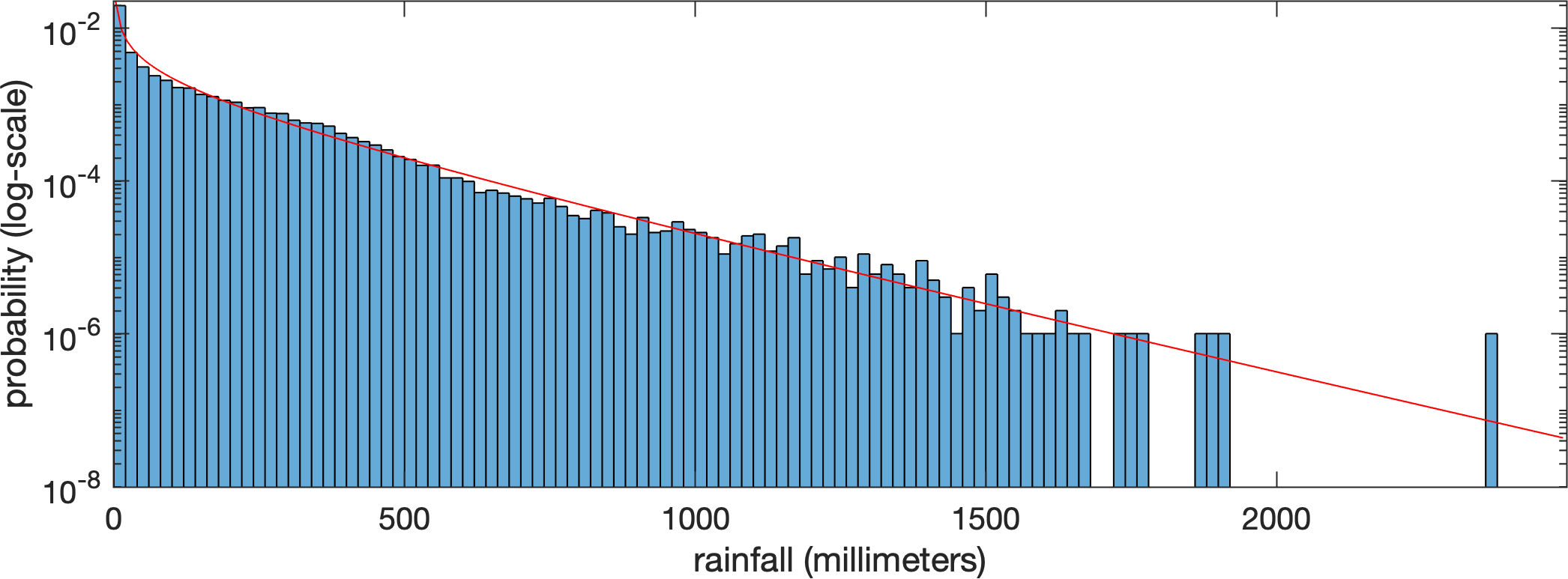
Figure 11: Histogram of monthly rainfall totals for 36 regions in India over 115 years. The estimated gamma distribution is shown in red.

A comparison of two GCP tensor decompositions is shown in Fig. 12. Factors in the first two modes (region and year) are normalized to length one, and the monthly factor is normalized by the size of the component. The rainfall from year to year follows no clear pattern, and this is consistent with the general understanding of these rainfall patterns. India is known for its monsoons, which occur in June–September of each year.

The GCP with standard Gaussian error loss and nonnegative constraints is shown in Fig. 12a. The first component captures the period July–September, which is the main part of the monsoon season. Components 3, 4, and 5 are dominated by a few regions. It is well known that Gaussian fitting can be swamped by outliers, and this may be the case here.

The GCP with the gamma distribution loss function is shown in Fig. 12b. This captures the monsoon season primarily in the first two components. There are no particular regions that dominate the factors.

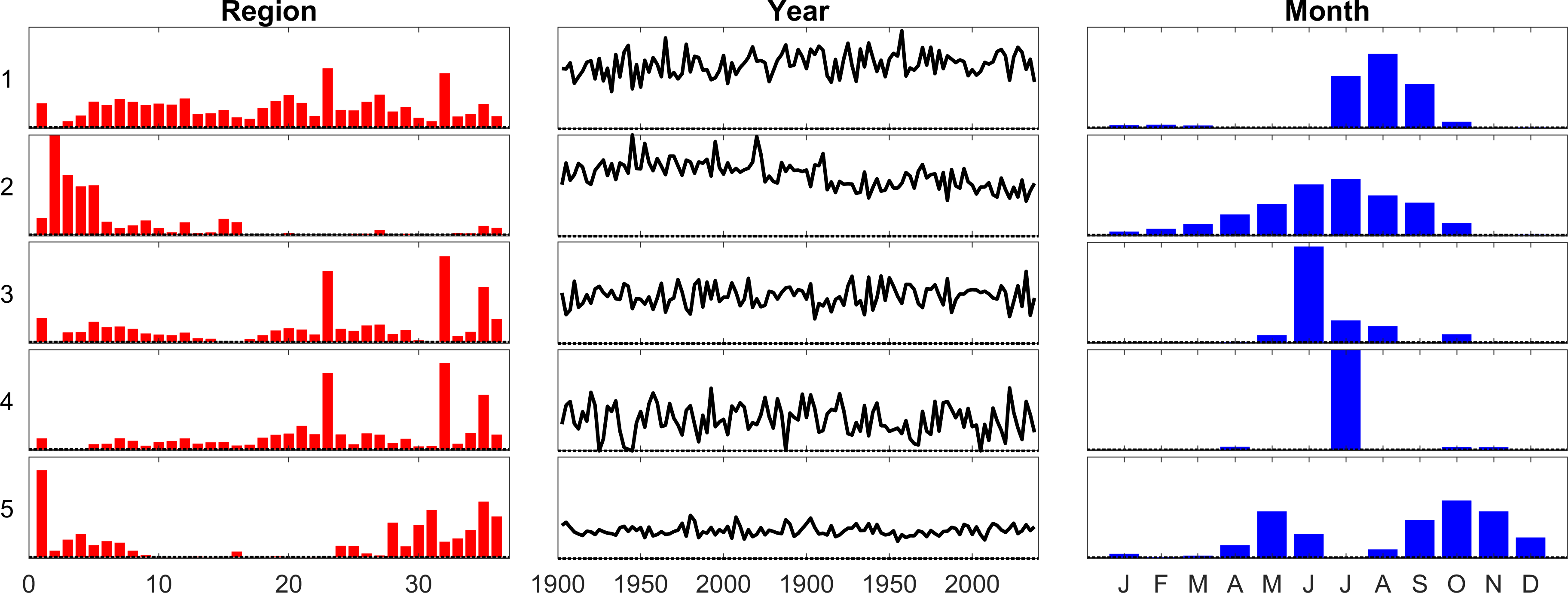
(a) Gaussian (standard CP) with nonnegativity constraints, which separates July into its own component.

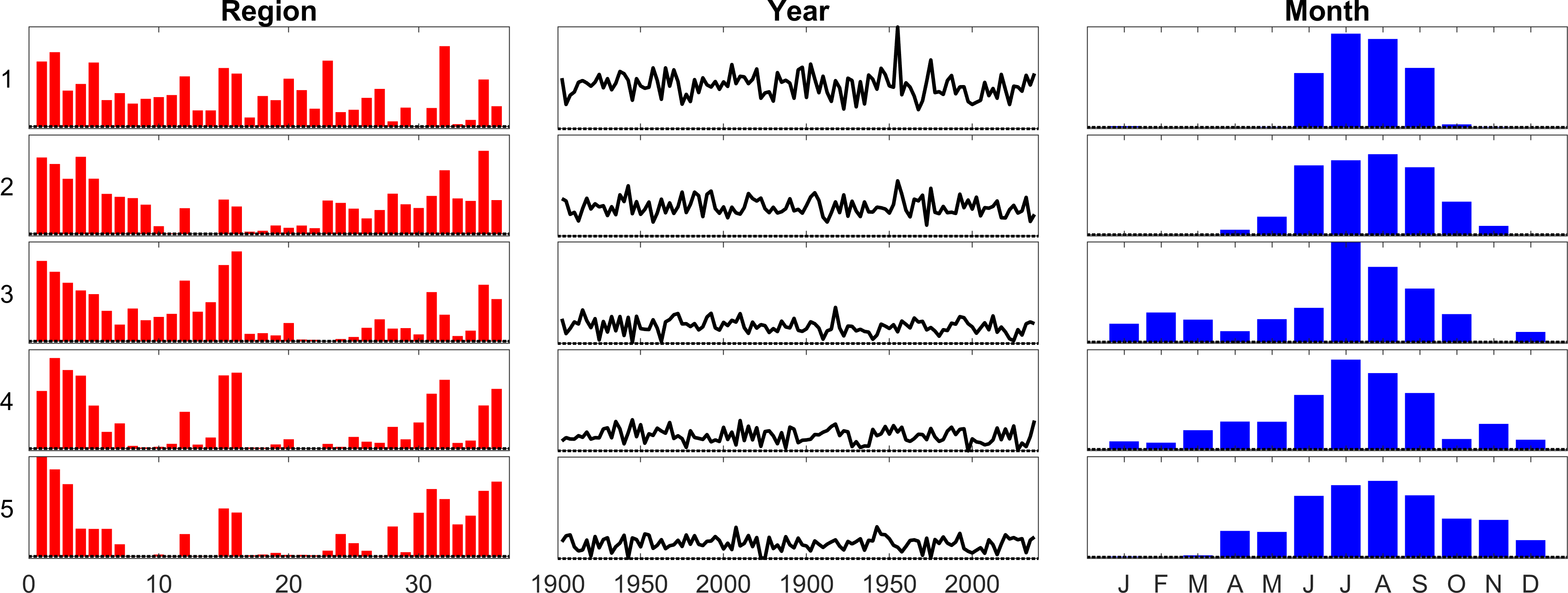
(b) Gamma (with nonnegativity constraints), which picks up the monsoon in the first component.

Figure 12: GCP tensor decomposition of India rainfall data, organized into a tensor of 36 regions, 115 years, and 12 months. The first two modes are normalized to length 1

6 Conclusions and future work

We have presented the GCP tensor decomposition framework which allows the use of an arbitrary elementwise loss function, generalizing previous works and enabling some extensions. GCP includes standard CP tensor decomposition and Poisson tensor decomposition [16], as well as decompositions based on beta divergences [19]. Using the GCP framework, we are able to define Bernoulli tensor decomposition for binary data, which is something like the tensor decomposition version of logistic regression and is derived via maximum likelihood. Alternatively, GCP can also handle a heuristic loss function such as Huber loss. We do not claim that any particular loss function is necessarily better than any other. Rather, for data analysis, it is often useful to have a variety of tools available, and GCP provides flexibility in terms of choosing among different loss functions to fit the needs of the analyst. Additionally, the GCP framework efficiently manages missing data, which is a common difficulty in practice. Our main theorem (Theorem 4.4) generalizes prior results for the gradient in the case of standard least squares, Poisson tensor factorization, and for missing data. It further reveals that the gradient takes the form of an MTTKRP, enabling the use of efficient implementations for this key tensor operation.

In our framework, we have proposed that the weights $w_{i}$ be used as indicators for missingness and restricted as $w_{i}\in\set{0,1}$. To generalize this, we can easily incorporate nonnegative elementwise weights $w_{i}\geq 0$. For instance, we might give higher or lower weights depending on the confidence in the data measurements. In recommender systems, there is also an idea that missing data may not be entirely missing at random. In this case, it may be useful to treat missing data elements as zeros but with low weights; see, e.g., [57].

For simplicity, our discussion focused on using the same elementwise loss function $f(x_{i},m_{i})$ for all entries of the tensor. However, we could easily define a different loss function for every entry, i.e., $f_{i}(x_{i},m_{i})$. The only modification is to the definition Eq. 30 of the elementwise derivative tensor $\bm{\mathscr{{Y}}}$. If we have a heterogeneous mixture of data types, this may be appropriate. In the matrix case, Udell, Horn, Zadeh, and Boyd [58] have proposed generalized low-rank models (GLRMs) which use a different loss function for each column in matrix factorization. We have also assumed our loss functions are continuously differentiable with respect to $m_{i}$, but that can potentially be relaxed as well in the same way as done by Udell et al. [58].

In our discussion of scarcity in Section 4.3, we alluded to the potential utility of imposing scarcity for scaling up to larger scale tensors. In stochastic gradient descent, for example, we impose scarcity by selecting only a few elements of the tensor at each iteration. Another option is to purposely omit most of the data, depending on the inherent redundancies in the data (assuming it is sufficiently incoherent). These are topics that we will investigate in detail in future work.

Lastly, it may also be of interest to extend the GCP framework to functional tensor decomposition. Garcke [25], e.g., has used hinge and Huber losses for fitting a functional version of the CP tensor decomposition.

Appendix A Kruskal tensors with explicit weights

It is sometimes convenient to write Eq. 6 with explicit positive weights ${\bm{\mathbf{{\lambda}}}}\in\mathbb{R}_{+}^{r}$, i.e.,

(33) $$m(i_{1},i_{2}\dots,i_{d})=\sum_{j=1}^{r}\lambda(j)\;a_{1}(i_{1},j)\,a_{2}(i_{2},j)\cdots a_{d}(i_{d},j),$$

with shorthand $\bm{\mathscr{{M}}}=\llbracket{\bm{\mathbf{{\lambda}}}};{\bm{\mathbf{{A}}}}_{1},{\bm{\mathbf{{A}}}}_{2},\dots,{\bm{\mathbf{{A}}}}_{d}\rrbracket$. In this case, the mode-$k$ unfolding in Eq. 7 is instead given by

$${\bm{\mathbf{{M}}}}_{(k)}={\bm{\mathbf{{A}}}}_{k}\operatorname{diag}({\bm{\mathbf{{\lambda}}}}){\bm{\mathbf{{Z}}}}_{k}^{T}.$$

We can also define the vectorized form

(34) $$\bm{\mathscr{{M}}}=\llbracket{\bm{\mathbf{{\lambda}}}};{\bm{\mathbf{{A}}}}_{1},{\bm{\mathbf{{A}}}}_{2},\dots,{\bm{\mathbf{{A}}}}_{d}\rrbracket\Rightarrow{\bm{\mathbf{{m}}}}={\bm{\mathbf{{Z}}}}\bm{\lambda},$$

where

(35) $${\bm{\mathbf{{Z}}}}\equiv{\bm{\mathbf{{A}}}}_{d}\odot{\bm{\mathbf{{A}}}}_{d-1}\odot\cdots\odot{\bm{\mathbf{{A}}}}_{1}\in\mathbb{R}^{n^{d}\times r}.$$

Using these definitions, it is a straightforward exercise to extend Theorem 4.4 to the case $\bm{\mathscr{{M}}}=\llbracket{\bm{\mathbf{{\lambda}}}};{\bm{\mathbf{{A}}}}_{1},{\bm{\mathbf{{A}}}}_{2},\dots,{\bm{\mathbf{{A}}}}_{d}\rrbracket$.

Corollary A.1.

Let the conditions of Theorem 4.4 hold except that the model has an explicit weight vector so that $\bm{\mathscr{{M}}}=\llbracket{\bm{\mathbf{{\lambda}}}};{\bm{\mathbf{{A}}}}_{1},{\bm{\mathbf{{A}}}}_{2},\dots,{\bm{\mathbf{{A}}}}_{d}\rrbracket$. In this case, the partial derivatives of $F$ w.r.t. ${\bm{\mathbf{{A}}}}_{k}$ and $\bm{\lambda}$ are

(36) $$\frac{\partial F}{\partial{\bm{\mathbf{{A}}}}_{k}missing}={\bm{\mathbf{{Y}}}}_{(k)}{\bm{\mathbf{{Z}}}}_{k}\operatorname{diag}(\bm{\lambda})\quad\text{and}\quad\frac{\partial F}{\partial\bm{\lambda}}={\bm{\mathbf{{Z}}}}^{T}{\bm{\mathbf{{y}}}},$$

where ${\bm{\mathbf{{Y}}}}_{(k)}$ and ${\bm{\mathbf{{y}}}}$ are, respectively, the mode-$k$ unfolding and vectorization of the tensor $\bm{\mathscr{{Y}}}$ defined in Eq. 30, ${\bm{\mathbf{{Z}}}}_{k}$ is defined in Eq. 7, and ${\bm{\mathbf{{Z}}}}$ is defined in Eq. 35.

Appendix B Special structure of standard CP gradient

In standard CP, which uses $f(x,m)=(x-m)^{2}$, the gradient has special structure that can be exploited when $\bm{\mathscr{{X}}}$ is sparse. Leaving out the constant, $\frac{\partial f}{\partial m}=-x+m$; therefore, $\bm{\mathscr{{Y}}}=-\bm{\mathscr{{X}}}+\bm{\mathscr{{M}}}$. From Eq. 29, the CP gradient is

(37) $$\frac{\partial F}{\partial{\bm{\mathbf{{A}}}}_{k}missing}=-({\bm{\mathbf{{X}}}}_{(k)}-{\bm{\mathbf{{M}}}}_{(k)}){\bm{\mathbf{{Z}}}}_{k}=-{\bm{\mathbf{{X}}}}_{(k)}{\bm{\mathbf{{Z}}}}_{k}+{\bm{\mathbf{{A}}}}_{k}({\bm{\mathbf{{Z}}}}_{k}^{\intercal}{\bm{\mathbf{{Z}}}}_{k}^{\phantom{\intercal}}).$$

The first term is an MTTKRP with the original tensor, and so it can exploit sparsity if $\bm{\mathscr{{X}}}$ is sparse, reducing the cost from $\mathcal{O}(rn^{d})$ to $\mathcal{O}(r^{2}d\cdot\text{nnz}(\bm{\mathscr{{X}}}))$ and avoiding forming ${\bm{\mathbf{{Z}}}}_{k}$ explicitly. The second term can also avoid forming ${\bm{\mathbf{{Z}}}}_{k}$ explicitly since its gram matrix is given by

(38) $${\bm{\mathbf{{Z}}}}_{k}^{\intercal}{\bm{\mathbf{{Z}}}}_{k}^{\phantom{\intercal}}=({\bm{\mathbf{{A}}}}_{1}^{\intercal}{\bm{\mathbf{{A}}}}_{1}^{\phantom{\intercal}})\ast\cdots\ast({\bm{\mathbf{{A}}}}_{k-1}^{\intercal}{\bm{\mathbf{{A}}}}_{k-1}^{\phantom{\intercal}})\ast({\bm{\mathbf{{A}}}}_{k+1}^{\intercal}{\bm{\mathbf{{A}}}}_{k+1}^{\phantom{\intercal}})\ast\cdots\ast({\bm{\mathbf{{A}}}}_{d}^{\intercal}{\bm{\mathbf{{A}}}}_{d}^{\phantom{\intercal}}),$$

where $\ast$ is the Hadamard (elementwise) product. This means that ${\bm{\mathbf{{Z}}}}_{k}^{\intercal}{\bm{\mathbf{{Z}}}}_{k}^{\phantom{\intercal}}$ is trivial to compute, requiring only $\mathcal{O}(r^{2}d\bar{n})$ operations. Equation 37 is a well-known result; see, e.g., [2]. Computation of MTTKRP with a sparse tensor is discussed further in [7].

Appendix C GCP optimization

First-order optimization methods expect a vector-valued function $f:\mathbb{R}^{n}\rightarrow\mathbb{R}$ and a corresponding vector-valued gradient, but our variable is the set of $d$ factor matrices. Because it may not be immediately obvious, we briefly explain how to make the conversion. We define the function kt2vec to convert a Kruskal tensor, i.e., a set of factor matrices, as follows:

$${\bm{\mathbf{{a}}}}\leftarrow\textsc{kt2vec}(\set{{\bm{\mathbf{{A}}}}_{k}missing}{k=1,\dots,d})\equiv\left[\textsc{vec}({\bm{\mathbf{{A}}}}_{1});\,\textsc{vec}({\bm{\mathbf{{A}}}}_{2});\,\dots;\,\textsc{vec}({\bm{\mathbf{{A}}}}_{d})\right].$$

The vec operator converts a matrix to a column vector by stacking its columns, and we use MATLAB-like semicolon notation to say that the kt2vec operator stacks all those vectors on top of each other. We can define a corresponding inverse operator, vec2kt. The number of variables in the set of factor matrices $\set{{\bm{\mathbf{{A}}}}_{k}missing}{k=1,\dots,d}$ is $dr\bar{n}$, and this is exactly the same number in the vector version ${\bm{\mathbf{{a}}}}$ because it is just a rearrangement of the entries in the factor matrices. Since the entries of the gradient matrices correspond to the same entries in the factor matrices, we use the same transformation function for them. The wrapper that would be used to call an optimization method is shown in Algorithm 2. The optimization method would input a vector optimization variable, this is converted to a sequence of matrices, we compute the function and gradient using Algorithm 1, we turn the gradients into a vector, and we return this along with the function value.

Algorithm 2 Wrapper for using first-order optimization method

1:function gcp_fg_wrapper(a)

2:     $\set{{\bm{\mathbf{{A}}}}_{k}missing}{k=1,\dots,d}\leftarrow\textsc{vec2kt}({\bm{\mathbf{{a}}}})$

3:     $[F,\set{{\bm{\mathbf{{G}}}}_{k}missing}{k=1,\dots,d}]\leftarrow\textsc{gcp\_fg}(\bm{\mathscr{{X}}},\Omega,\set{{\bm{\mathbf{{A}}}}_{k}missing}{k=1,\dots,d})$

4:     ${\bm{\mathbf{{g}}}}\leftarrow\textsc{kt2vec}(\set{{\bm{\mathbf{{G}}}}_{k}missing}{k=1,\dots,d})$

5:     return $[F,{\bm{\mathbf{{g}}}}]$

6:end function

Appendix D Acknowledgments

We would like to acknowledge the contributions of our colleague Cliff Anderson-Bergman, who served as a mentor to David Hong in this work. Thanks for Age Smilde for suggesting negative binomial, to Michiel Vandecappelle for inspiring the discussion of beta divergences, and to Martin Mohlenkamp for making us aware of the work by Garcke [25]. Thanks to Brett Larsen for feedback on earlier drafts of this work. We are extremely grateful to the anonymous referees for critical feedback that led to significant improvements.

References

- [1] E. Acar, C. A. Bingol, H. Bingol, R. Bro, and B. Yener, Multiway analysis of epilepsy tensors, Bioinformatics, 23 (2007), pp. i10–i18, doi:10.1093/bioinformatics/btm210.
- [2] E. Acar, D. M. Dunlavy, and T. G. Kolda, A scalable optimization approach for fitting canonical tensor decompositions, Journal of Chemometrics, 25 (2011), pp. 67–86, doi:10.1002/cem.1335.
- [3] E. Acar, D. M. Dunlavy, T. G. Kolda, and M. Mørup, Scalable tensor factorizations with missing data, in SDM10: Proceedings of the 2010 SIAM International Conference on Data Mining, 2010, pp. 701–712, doi:10.1137/1.9781611972801.61.
- [4] E. Acar, D. M. Dunlavy, T. G. Kolda, and M. Mørup, Scalable tensor factorizations for incomplete data, Chemometrics and Intelligent Laboratory Systems, 106 (2011), pp. 41–56, doi:10.1016/j.chemolab.2010.08.004.
- [5] E. Acar and B. Yener, Unsupervised multiway data analysis: A literature survey, IEEE Transactions on Knowledge and Data Engineering, 21 (2009), pp. 6–20, doi:10.1109/TKDE.2008.112.
- [6] B. W. Bader and T. G. Kolda, Algorithm 862: MATLAB tensor classes for fast algorithm prototyping, ACM Transactions on Mathematical Software, 32 (2006), pp. 635–653, doi:10.1145/1186785.1186794.
- [7] B. W. Bader and T. G. Kolda, Efficient MATLAB computations with sparse and factored tensors, SIAM Journal on Scientific Computing, 30 (2007), pp. 205–231, doi:10.1137/060676489.
- [8] B. W. Bader, T. G. Kolda, et al., MATLAB Tensor Toolbox Version 3.0-dev. Available online, Oct. 2017, https://www.tensortoolbox.org.
- [9] G. Ballard, N. Knight, and K. Rouse, Communication lower bounds for matricized tensor times Khatri-Rao product, 2017, arXiv:1708.07401v1 [cs.DC].
- [10] G. Beylkin, J. Garcke, and M. J. Mohlenkamp, Multivariate regression and machine learning with sums of separable functions, SIAM Journal on Scientific Computing, 31 (2009), pp. 1840–1857, doi:10.1137/070710524.
- [11] G. Beylkin and M. J. Mohlenkamp, Numerical operator calculus in higher dimensions, Proceedings of the National Academy of Sciences, 99 (2002), pp. 10246–10251, doi:10.1073/pnas.112329799.
- [12] G. Beylkin and M. J. Mohlenkamp, Algorithms for numerical analysis in high dimensions, SIAM Journal on Scientific Computing, 26 (2005), pp. 2133–2159, doi:10.1137/040604959.
- [13] R. Bro, PARAFAC. Tutorial and applications, Chemometrics and Intelligent Laboratory Systems, 38 (1997), pp. 149–171, doi:10.1016/S0169-7439(97)00032-4.
- [14] R. H. Byrd, P. Lu, J. Nocedal, and C. Zhu, A limited memory algorithm for bound constrained optimization, SIAM J. Sci. Comput., 16 (1995), pp. 1190–1208, doi:10.1137/0916069.
- [15] J. D. Carroll and J. J. Chang, Analysis of individual differences in multidimensional scaling via an N-way generalization of “Eckart-Young” decomposition, Psychometrika, 35 (1970), pp. 283–319, doi:10.1007/BF02310791.
- [16] E. C. Chi and T. G. Kolda, On tensors, sparsity, and nonnegative factorizations, SIAM Journal on Matrix Analysis and Applications, 33 (2012), pp. 1272–1299, doi:10.1137/110859063.
- [17] A. Cichocki and S. ichi Amari, Families of alpha- beta- and gamma- divergences: Flexible and robust measures of similarities, Entropy, 12 (2010), pp. 1532–1568, doi:10.3390/e12061532.
- [18] A. Cichocki and A.-H. Phan, Fast local algorithms for large scale nonnegative matrix and tensor factorizations, IEICE Transactions on Fundamentals of Electronics, Communications and Computer Sciences, E92.A (2009), pp. 708–721, doi:10.1587/transfun.E92.A.708.
- [19] A. Cichocki, R. Zdunek, S. Choi, R. Plemmons, and S.-I. Amari, Non-negative tensor factorization using alpha and beta divergences, in ICASSP 07: Proceedings of the International Conference on Acoustics, Speech, and Signal Processing, 2007, doi:10.1109/ICASSP.2007.367106.
- [20] M. Collins, S. Dasgupta, and R. E. Schapire, A generalization of principal components analysis to the exponential family, in NIPS’02: Advances in Neural Information Processing Systems 14, MIT Press, 2002, pp. 617–624, http://papers.nips.cc/paper/2078-a-generalization-of-principal-components-analysis-to-the-exponential-family.pdf.
- [21] F. Cong, Q.-H. Lin, L.-D. Kuang, X.-F. Gong, P. Astikainen, and T. Ristaniemi, Tensor decomposition of EEG signals: A brief review, Journal of Neuroscience Methods, 248 (2015), pp. 59–69, doi:10.1016/j.jneumeth.2015.03.018.
- [22] D. M. Dunlavy, T. G. Kolda, and E. Acar, Temporal link prediction using matrix and tensor factorizations, ACM Transactions on Knowledge Discovery from Data, 5 (2011), p. 10 (27 pages), doi:10.1145/1921632.1921636.
- [23] L. Fang, N. He, and H. Lin, CP tensor-based compression of hyperspectral images, Journal of the Optical Society of America A, 34 (2017), pp. 252–258, doi:10.1364/josaa.34.000252.
- [24] C. Févotte and J. Idier, Algorithms for nonnegative matrix factorization with the -divergence, Neural Computation, 23 (2011), pp. 2421–2456, doi:10.1162/NECO_a_00168.
- [25] J. Garcke, Classification with sums of separable functions, in Machine Learning and Knowledge Discovery in Databases, J. L. Balcázar, F. Bonchi, A. Gionis, and M. Sebag, eds., Springer Berlin Heidelberg, 2010, pp. 458–473, doi:10.1007/978-3-642-15880-3_35.
- [26] G. J. Gordon, Generalized2 linear2 models, in Advances in Neural Information Processing Systems (NIPS’03), 2003, pp. 593–600.
- [27] W. Hackbusch and B. N. Khoromskij, Tensor-product approximation to operators and functions in high dimensions, Journal of Complexity, 23 (2007), pp. 697–714, doi:10.1016/j.jco.2007.03.007.
- [28] S. Hansen, T. Plantenga, and T. G. Kolda, Newton-based optimization for Kullback-Leibler nonnegative tensor factorizations, Optimization Methods and Software, 30 (2015), pp. 1002–1029, doi:10.1080/10556788.2015.1009977, arXiv:1304.4964.
- [29] R. A. Harshman, Foundations of the PARAFAC procedure: Models and conditions for an “explanatory” multi-modal factor analysis, UCLA working papers in phonetics, 16 (1970), pp. 1–84. Available at http://www.psychology.uwo.ca/faculty/harshman/wpppfac0.pdf.
- [30] T. Hastie, R. Tibshrirani, and J. Friedman, The Elements of Statitical Learning, Springer, 2nd ed., 2009, doi:10.1007/978-0-387-84858-7.
- [31] K. Hayashi, G. Ballard, J. Jiang, and M. Tobia, Shared memory parallelization of MTTKRP for dense tensors, 2017, arXiv:1708.08976v1 [cs.DC].
- [32] F. L. Hitchcock, The expression of a tensor or a polyadic as a sum of products, Journal of Mathematics and Physics, 6 (1927), pp. 164–189, doi:10.1002/sapm192761164.
- [33] K. Huang, N. D. Sidiropoulos, and A. P. Liavas, A flexible and efficient algorithmic framework for constrained matrix and tensor factorization, IEEE Transactions on Signal Processing, 64 (2016), pp. 5052–5065, doi:10.1109/TSP.2016.2576427, arXiv:1506.04209v2.
- [34] P. J. Huber, Robust estimation of a location parameter, Annals of Statistics, 53 (1964), pp. 73–101, doi:10.1214/aoms/1177703732.
- [35] R. Jaffé, K. M. Cawley, and Y. Yamashita, Applications of excitation emission matrix fluorescence with parallel factor analysis (EEM-PARAFAC) in assessing environmental dynamics of natural dissolved organic matter (DOM) in aquatic environments: A review, in Advances in the Physicochemical Characterization of Dissolved Organic Matter: Impact on Natural and Engineered Systems, vol. 1160 of ACS Symposium Series, American Chemical Society (ACS), 2014, pp. 27–73, doi:10.1021/bk-2014-1160.ch003.
- [36] T. Kolda and B. Bader, The TOPHITS model for higher-order web link analysis, in Proceedings of Link Analysis, Counterterrorism and Security 2006, 2006, http://www.siam.org/meetings/sdm06/workproceed/Link%****␣paper.tex␣Line␣2350␣****Analysis/21Tamara_Kolda_SIAMLACS.pdf.
- [37] T. G. Kolda, Sparse versus scarce. Blog, Nov. 2017, http://www.kolda.net/post/sparse-versus-scarce/. Accessed May 2018.
- [38] T. G. Kolda and B. W. Bader, Tensor decompositions and applications, SIAM Review, 51 (2009), pp. 455–500, doi:10.1137/07070111X.
- [39] D. D. Lee and H. S. Seung, Learning the parts of objects by non-negative matrix factorization, Nature, 401 (1999), pp. 788–791, doi:10.1038/44565.
- [40] J. Li, Y. Ma, C. Yan, and R. Vuduc, Optimizing sparse tensor times matrix on multi-core and many-core architectures, in Workshop on Irregular Applications: Architecture and Algorithms (IA3), 2016, pp. 26–33, doi:10.1109/IA3.2016.010.
- [41] K. Maruhashi, F. Guo, and C. Faloutsos, MultiAspectForensics: Pattern mining on large-scale heterogeneous networks with tensor analysis, in 2011 International Conference on Advances in Social Networks Analysis and Mining (ASONAM), IEEE, 2011, pp. 203–210, doi:10.1109/asonam.2011.80.
- [42] K. R. Murphy, C. A. Stedmon, D. Graeber, and R. Bro, Fluorescence spectroscopy and multi-way techniques. PARAFAC, Analytical Methods, 5 (2013), p. 6557, doi:10.1039/c3ay41160e.
- [43] M. Nickel and V. Tresp, Logistic tensor factorization for multi-relational data, 2013, arXiv:1306.2084v1 [stat.ML].
- [44] T. Opsahl, Network 1: Facebook-like social network, https://toreopsahl.com/datasets/#online_social_network (accessed 2018-06-20).
- [45] T. Opsahl and P. Panzarasa, Clustering in weighted networks, Social Networks, 31 (2009), pp. 155–163, doi:10.1016/j.socnet.2009.02.002, https://doi.org/10.1016/j.socnet.2009.02.002.
- [46] P. Paatero, Least squares formulation of robust non-negative factor analysis, Chemometrics and Intelligent Laboratory Systems, 37 (1997), pp. 23–35, doi:10.1016/S0169-7439(96)00044-5.
- [47] P. Paatero, A weighted non-negative least squares algorithm for three-way “PARAFAC” factor analysis, Chemometrics and Intelligent Laboratory Systems, 38 (1997), pp. 223–242, doi:10.1016/S0169-7439(97)00031-2.
- [48] P. Paatero and U. Tapper, Positive matrix factorization: A non-negative factor model with optimal utilization of error estimates of data values, Environmetrics, 5 (1994), pp. 111–126, doi:10.1002/env.3170050203.
- [49] P. Panzarasa, T. Opsahl, and K. M. Carley, Patterns and dynamics of users' behavior and interaction: Network analysis of an online community, Journal of the American Society for Information Science and Technology, 60 (2009), pp. 911–932, doi:10.1002/asi.21015, https://doi.org/10.1002/asi.21015.
- [50] E. E. Papalexakis, U. Kang, C. Faloutsos, N. D. Sidiropoulos, and A. Harpale, Large scale tensor decompositions: Algorithmic developments and applications, IEEE Data Eng. Bull., 36 (2013), pp. 59–66, http://sites.computer.org/debull/A13sept/p59.pdf.
- [51] A.-H. Phan, P. Tichavsky, and A. Cichocki, Fast alternating LS algorithms for high order CANDECOMP/PARAFAC tensor factorizations, IEEE Transactions on Signal Processing, 61 (2013), pp. 4834–4846, doi:10.1109/TSP.2013.2269903, http://dx.doi.org/10.1109/TSP.2013.2269903.
- [52] A.-H. Phan, P. Tichavský, and A. Cichocki, Low complexity damped Gauss–Newton algorithms for CANDECOMP/PARAFAC, SIAM Journal on Matrix Analysis and Applications, 34 (2013), pp. 126–147, doi:10.1137/100808034, http://dx.doi.org/10.1137/100808034.
- [53] S. Rendle, Factorization machines with libFM, ACM Transactions on Intelligent Systems and Technology (TIST), 3 (2012), 57 (22 pages), pp. 57:1–57:22, doi:10.1145/2168752.2168771, http://doi.acm.org/10.1145/2168752.2168771.
- [54] M. J. Reynolds, A. Doostan, and G. Beylkin, Randomized alternating least squares for canonical tensor decompositions: Application to a PDE with random data, SIAM Journal on Scientific Computing, 38 (2016), pp. A2634–A2664, doi:10.1137/15M1042802.
- [55] A. Shashua and T. Hazan, Non-negative tensor factorization with applications to statistics and computer vision, in ICML 2005: Proceedings of the 22nd International Conference on Machine Learning, 2005, pp. 792–799, doi:10.1145/1102351.1102451.
- [56] S. Smith and G. Karypis, Tensor-matrix products with a compressed sparse tensor, in Proceedings of the 5th Workshop on Irregular Applications: Architectures and Algorithms, ACM, 2015, p. 7.
- [57] H. Steck, Training and testing of recommender systems on data missing not at random, in KDD’10: Proceedings of the 16th ACM SIGKDD International Conference on Knowledge Discovery and Data Mining, 2010, pp. 713–722, doi:10.1145/1835804.1835895.
- [58] M. Udell, C. Horn, R. Zadeh, and S. Boyd, Generalized low rank models, FNT in Machine Learning, 9 (2016), pp. 1–118, doi:10.1561/2200000055, http://dx.doi.org/10.1561/2200000055.
- [59] M. Welling and M. Weber, Positive tensor factorization, Pattern Recognition Letters, 22 (2001), pp. 1255–1261, doi:10.1016/S0167-8655(01)00070-8.
- [60] A. H. Williams, T. H. Kim, F. Wang, S. Vyas, S. I. Ryu, K. V. Shenoy, M. Schnitzer, T. G. Kolda, and S. Ganguli, Unsupervised discovery of demixed, low-dimensional neural dynamics across multiple timescales through tensor components analysis, Neuron, 98 (2018), pp. 1099–1115, doi:10.1016/j.neuron.2018.05.015.
- [61] G. Young, Maximum likelihood estimation and factor analysis, Psychometrika, 6 (1941), pp. 49–53, doi:10.1007/bf02288574.
- [62] Q. Zhang, H. Wang, R. J. Plemmons, and V. P. Pauca, Tensor methods for hyperspectral data analysis: a space object material identification study, J. Opt. Soc. Am. A, 25 (2008), pp. 3001–3012, doi:10.1364/JOSAA.25.003001, http://josaa.osa.org/abstract.cfm?URI=josaa-25-12-3001.