Joule-Thomson expansion in AdS black holes with momentum relaxation

Abstract

The inner structure of realistic materials make them exhibit momentum relaxation. In this paper we study the Joule-Thomson effect on AdS black holes in which translational invariance is broken by two methods: First by considering planar black holes in general relativity supported by scalar fields with a linear dependence on the horizon coordinates and secondly by considering black holes in massive gravity models in which momentum relaxation is obtained by breaking the bulk diffeomorphism invariance of the theory. In contrast with black holes studied so far, for both theories it is possible to obtain inversion curves with two branches reproducing the behavior of Van der Waals fluids. Moreover in the specific case of the massive gravity model we show that black holes can heat up when crossing the inversion curve.

I Introduction

From the very beginning black holes were described as extreme classical objects that absorb every kind of matter and energy without leaving anything out. Basically regarded as bald objects Ruffini:1971bza ; Bekenstein:1998aw they were supposed to be described just by few parameters; mass, angular momentum and electromagnetic charges. With the advent of quantum field theory, particularly in the context of curved spacetimes, it was demonstrated the fundamental relationship existing between the area of black holes and their entropy entropy1 and that they possess a temperature related with its surface gravity tem1 . Moreover it was shown that black holes emit radiation resembling the spectrum of black bodies. All these considerations led to the development of black hole thermodynamics termo1 , constituting the first successful semiclassical description of gravitational phenomena, a deep insight into the understanding of a possible quantum description of the gravitational interaction.

When considering black holes in Anti-de Sitter spacetimes black hole thermodynamics becomes particularly interesting. The AdS/CFT correspondence defines a duality between gravitational theories on anti-de Sitter spacetimes in $(D+1)-$dimensions and conformal field theories in $D-$dimensions Maldacena . In this context black holes in the presence of a negative cosmological constant admits a dual description given by thermal states in a conformal field theory. Hawking and Page HPT demonstrated that AdS spacetimes suffer a phase transition from the AdS background state to large Schwarzschild AdS black holes for a critical temperature. Phase transition that was demonstrated to be dual to a confinement/deconfinement phase transition in the free energy of the dual field theory quark/gluon plasma Witten:1998qj ; witten2 . Many applications of these ideas that combine black hole thermodynamics and AdS/CFT duality have been developed during the last decade providing a deeper understanding of the interplay between gravity and quantum physics in the context of condense matter physics, hart1 ; hart2 , the loss information paradox info1 , quantum chromodynamics cromo1 , to mention few examples.

When considering black hole thermodynamic for AdS black holes the cosmological constant parameter, $\Lambda$, is considered as a fixed parameter introduced in the action and does not appears in the first law of black hole thermodynamics. This ensures that we are comparing thermodynamical ensembles for solutions exhibiting the same asymptotic behavior, by fixing the AdS background.

Despite its original constant nature, it is interesting to explore how black hole thermodynamic is modified when considering the cosmological constant, $\Lambda$, as a thermodynamical variable Kastor:2009wy ; lam2 . In fact, the cosmological constant, from a perfect fluid point of view incorpores the notion of Pressure, through the relation

$$P=-\frac{\Lambda}{8\pi}=\frac{(d-1)(d-2)}{16\pi l^{2}}$$ (1)

where $d$ represents the dimension of the spacetime and $l$ the AdS radius. This allows to obtain a more physical interpretation of what the volume of a black hole should be lam3 ; lam4 , thermodynamical volume defined by

$$V=\left(\frac{\partial{M}}{\partial{P}}\right)_{S,J,Q}.$$ (2)

This permits the inclusion of the pressure-volume term of everyday thermodynamic $PV$ into the first law of black hole thermodynamic Dolan:2012jh , term that does not appears otherwise. Moreover provides the correct Smarr relation for AdS black holes delivering a concrete expression relating extensive and intensive thermodynamic variables. In this case the mass $M$ of the spacetime must be interpreted as the enthalpy of the thermodynamical system Kastor:2009wy . Novel new phenomenology is obtained, new phase transitions like Van der Waals liquid-gas phase transitions mann1 ; mann2 , existence of triple points like the one encountered in the phase diagram of water Kubiznak:2016qmn , heat engines black hole analogous, just to mention few applications Johnson:2014yja ; Hennigar:2017apu ; Fang:2017nse ; Hu:2019wwn . The subject has been dubbed generalized black hole thermodynamic or black hole chemistry Kubiznak:2016qmn .

An interesting classical thermodynamical effect is the so-called Joule-Thomson effect, also known as Joule-Thomson expansion Ref-JT . This effect deals with the change of temperature of a gas or fluid when it is expanded adiabatically by using a valve. In fact this adiabatic expansion can be performed in several ways. The Joule-Thomson effect takes place when the thermodynamical process occurring during the expansion is irreversible and enthalpy remains constant. The change of temperature is measured by the Joule-Thomson coefficient $\mu_{JT}$ which can be either positive or negative depending if the fluid is cooling or heating, respectively.

By working on the context of generalized black hole thermodynamic recently the Joule-Thomson effect have been studied for first time by Ökcü and Aydıner Okcu:2016tgt , in particular for the case of Reissner-Nordstrom black holes in anti-de Sitter spacetimes.

As we have stated previously, the Joule-Thomson expansion deals with the change of temperature of the fluid under expansion in an isenthalpic process. This change is quantitatively expressed by the sign of the Joule-Thomson coefficient defined by Ref-JT

$$\mu_{JT}=\left(\frac{\partial T}{\partial P}\right)_{H}.$$ (3)

We observe that by computing this coefficient it is possible to determinate when heating or cooling is taking place. Even if pressure is always decreasing the change of temperature can be either positive or negative. When $\mu_{JT}$ goes to zero it is possible to defined the inversion temperature $T_{i}$, the particular point in the gradient of temperature of the black hole for which the system change from cooling to heating or vice versa. In the same manner it is defined the inversion pressure $P_{i}$. Then $(P_{i},T_{i})$ gives inversion transition point. By making use of the generalized first law of black hole thermodynamic and taking into account the isenthalpic nature of the process, it is possible to define the Joule-Thomson coefficient in term of the volume and heat capacity at constant pressure Okcu:2016tgt ,

$$\mu_{JT}=\left(\frac{\partial T}{\partial P}\right)_{H}=\frac{1}{C_{P}}\left[T\left(\frac{\partial V}{\partial T}\right)_{P}-V\right],$$ (4)

where $C_{P}=T\left(\frac{\partial S}{\partial T}\right)_{P}$ is the heat capacities at constant pressure. This definition has the advantage that allows to define easily the inversion temperature

$$T_{i}=V\left(\frac{\partial T}{\partial V}\right)_{P}$$ (5)

which will provide heating and cooling regions in the $T-P$ plane.

The study of Joule-Thomson expansion has been generalized for several black hole solutions including Quintessence AdS black hole Ghaffarnejad:2018exz , arbitrary dimensional charge AdS black hole Mo:2018rgq , Kerr-AdS black holes Okcu:2017qgo , Kerr-Newman-AdS black holesZhao:2018kpz ,Gauss-Bonnet AdS black holes Lan:2018nnp , Lovelock gravity Mo:2018qkt and nonlinear electrodynamic gravity Kuang:2018goo to mention few examples.

It is known that real materials exhibit momentum dissipation, namely, that momentum is not continuously conserved. This implies that resistivity of materials has a non-vanishing value providing for finite electrical conductivities. When making use of the tools of the gauge/gravity duality to study condense matter systems in term of their gravitational dual it is not straightforward to include momentum dissipation. At this respect to well-known strategies to produce momentum dissipation are the inclusion of matter fields that breaks translation invariance in the dual field theory, as it is for example the case of the scalar fields that depend linearly on the horizon coordinates Andrade:2013gsa , and the case of massive gravity theories which present a broken diffeomorphism invariance in the bulk Vegh:2013sk .

In this paper we present the study of the Joule-Thomson effect for two models presenting momentum dissipation: $(i)$ the Einstein-Maxwell-scalar theory where the scalar fields act as spatial-dependent sources breaking the Ward identity so that the momentum is not conserved in the dual theory Andrade:2013gsa ; $(ii)$ massive gravity theory where the momentum dissipation in the dual theory is implemented by breaking the diffeomorphism invariance in the bulk Vegh:2013sk . We will work in the units with $G=c=\hbar=k_{B}=1$.

The paper is organized as follows. Sec. II is designated to analyze the Joule-Thomson expansion in the context of Einstein-Maxwell-scalar theory. This is done for scalar fields presenting a standard kinetic term but also for the case in which the kinetic term is modified by the so-called k-essence term Baggioli:2014roa ; Cisterna:2017jmv . Sec. III is devoted to the analysis of the Joule-Thomson expansion in the context of massive gravity theory. Finally we conclude in Sec. IV.

II Joule-Thomson expansion in Einstein-Maxwell-scalars theory

II.1 Black holes in Einstein-Maxwell-scalars theory

The Einstein-Maxwell-scalars gravity theory with scalar fields was first proposed in Andrade:2013gsa by homogeneously distributing $2$ massless scalar fields along the horizon coordinates. The action principle in four dimensions reads

$$S=\frac{1}{16\pi G}\int\!d^{4}x\sqrt{-g}\left(R-2\Lambda-\frac{1}{4}F_{\mu\nu}F^{\mu\nu}-\frac{1}{2}\sum_{i=1}^{2}(\partial\psi_{i})^{2}\right)\ ,$$ (6)

where the cosmological and the AdS radius are related by $l^{2}=-\frac{3}{\Lambda}$.

By setting the scalar fields to depend on the $2$ dimensional spatial coordinates and by considering a spacetime with a planar base manifold the Klein-Gordon equation for the scalars is easily integrated, yielding

$$\psi_{I}=\beta_{Ia}x^{a}.$$ (7)

Subsequently one finds that the action admits the following charged black hole solution

$$ds^{2}=-f(r)dt^{2}+\frac{1}{f(r)}dr^{2}+r^{2}dx^{a}dx^{a},~{}~{}~{}~{}~{}A=A_{t}(r)dt,~{}~{}\mathrm{with}$$

$$f(r)=\frac{r^{2}}{l^{2}}-\frac{\beta^{2}}{2}-\frac{m}{r}+\frac{q^{2}}{r^{2}},~{}~{}~{}A_{t}=\left(1-\frac{r_{h}}{r}\right)\frac{2q}{r_{h}}$$ (8)

where the index $a$ goes $a=1,2$, and the horizon $r_{h}$ satisfies $f(r_{h})=0$. It is worthwhile to point out that the scalar fields in the bulk source a spatially dependent field theory with momentum relaxation, which is dual to the homogeneous and isotropic black hole (II.1) . The linear coefficient $\beta$ of the scalar fields somehow can be considered to describe the strength of the momentum relaxation in the boundary theory Andrade:2013gsa .

The mass and the charge of this black hole can be found by means of the Hamiltonian analysis or by using the holographic renormalization approach developed in Bardoux:2012aw ; Andrade:2013gsa . In there has been shown that the mass and charge of the black hole are connected with the parameters $m$ and $q$ as

$$M=\frac{\mathscr{V}_{2}}{8\pi}m,~{}~{}~{}\mathrm{and}~{}~{}~{}Q=\frac{\mathscr{V}_{2}}{8\pi}q$$ (9)

where $\mathscr{V}_{2}$ is the volume of the $2$ dimensional flat space and we will set it to be $1$. On the other hand, by identifying the period of the Euclidean time in order to avoid conical singularities, the temperature of the black hole is given by

$$T=\frac{f^{\prime}(r_{h})}{4\pi}=\frac{1}{4\pi}\left(\frac{3r_{h}}{l^{2}}-\frac{\beta^{2}}{2r_{h}}-\frac{q^{2}}{r_{h}^{3}}\right),$$ (10)

and the entropy is obtained by the area law as

$$S=\frac{r_{h}^{2}}{4}.$$ (11)

II.2 Joule-Thomson expansion

We shall apply the previous solution to the study of the Joule-Thomson expansion. To do so we consider the thermodynamical analysis of the Einstein-Maxwell-scalar theory provided in Fang:2017nse in which the cosmological constant is consider as a thermodynamical parameter susceptible to variations. The first law of black hole mechanics/thermodynamic under this approach has been properly identified by means of the hamiltonian formalism in Kastor:2009wy . It is important to stress that even if this upgrade of the original parameter nature of the cosmological constant is done straightforwardly, this can be done following the approach developed in the seminal paper Henneaux:1984ji where the cosmological constant is given by the inclusion of a three-index antisymmetric Abelian gauge field, which once integrated promote the cosmological constant to a canonical variable. Nevertheless it is fair to establishes that this is a subject of debate and that so far this treatment can be considered as a proposal more than a fundamental conjecture, indeed it offers many applications in black hole thermodynamics in close analogy with common thermodynamics but it has some subtleties when applying the full AdS/CFT dictionary.

As it is known the pressure is given by

$$P=-\frac{\Lambda}{8\pi}=\frac{3}{8\pi l^{2}}.$$ (12)

Making use of this result into the definition of mass, the mass of the black hole can be rewritten as

$$M=\frac{Pr_{h}^{3}}{3}+\frac{q^{2}}{8\pi r_{h}}-\frac{\beta^{2}r_{h}}{16\pi}$$ (13)

which is taken as the enthalpy $H$ of the system. On the other hand, let us use pressure (12) into the expression for the temperature (10), then

$$P=\frac{T}{2r_{h}}+\frac{\beta^{2}}{16\pi r_{h}^{2}}+\frac{q^{2}}{8\pi r_{h}^{4}}\ .$$ (14)

In this manner we obtain our black hole equation of state. The thermodynamical volume is the conjugate variable of the pressure, then

$$V=\left(\frac{\partial M}{\partial P}\right)_{Q,S}=\frac{r_{h}^{3}}{3}.$$ (15)

With these ingredients at hand we use the definition of the Joule-Thomson coefficient (4), obtaining

$$\mu_{JT}=\frac{2r_{h}\left(r_{h}^{2}\left(\beta^{2}+16\pi Pr_{h}^{2}-24\pi Tr_{h}\right)+6q^{2}\right)}{-48\pi Pr_{h}^{4}+3\beta^{2}r_{h}^{2}+6q^{2}}.$$ (16)

As was stated before, the point $\mu_{JT}$=0 defines the inversion temperature $T_{i}$, which in our case reads

$$T_{i}=\frac{16\pi P_{i}r_{h}^{4}+\beta^{2}r_{h}^{2}+6q^{2}}{24\pi r_{h}^{3}}$$ (17)

with the corresponding pressure $P_{i}$. As we see this expression depends apart from the inversion pressure on the horizon of the black hole. Nevertheless $r_{h}$ can be obtained from the temperature relation, relation that $T_{i}$ and $P_{i}$ must also satisfy, then the only positive root is

$$r_{h}=\frac{1}{4}\sqrt{\frac{\sqrt{\beta^{4}+96\pi P_{i}q^{2}}}{\pi P_{i}}+\frac{\beta^{2}}{\pi P_{i}}}.$$ (18)

Substituting (18) into (17), we obtain the analytical relation between the inversion temperature and pressure

$$T_{i}=\frac{\beta^{4}+\beta^{2}\sqrt{\beta^{4}+96\pi P_{i}q^{2}}+64\pi P_{i}q^{2}}{2\sqrt{\pi}P_{i}\left(\frac{\beta^{2}+\sqrt{\beta^{4}+96\pi P_{i}q^{2}}}{P_{i}}\right)^{3/2}}.$$ (19)

From this last equation we observe some analytical properties of the inversion temperature. For the case without momentum relaxation, i.e, $\beta=0$, we have $T_{i}=\frac{2\sqrt[4]{\frac{2}{\pi}}P_{i}^{3/4}\sqrt{q}}{3^{3/4}}$ which is proportional to $P_{i}^{3/4}$ with fixed $q\neq 0$. This shows that for planar charged AdS black holes the minimum temperature goes to zero when the inversion pressure tends to zero, contrary to the case in which the horizon is spherical. Moreover there is no inversion temperature for uncharged solutions. On the other hand when $q=0$, but we have momentum relaxation we obtain that $T_{i}=\frac{\mid\beta\mid\sqrt{P_{i}}}{2\sqrt{2\pi}}$ which is shifted from zero in contrast with the standard uncharged AdS black hole Okcu:2016tgt . We show the explicit relation of inversion curve for different $\beta$ in figure 1.

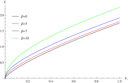
Figure 1: Inversion curves $T_{i}-P_{i}$ for heating and cooling processes for different values of $\beta$. We set $q=5$.

There is only one branch of inversion curves as that studied in Okcu:2016tgt ; Mo:2018qkt ; Lan:2018nnp ; Okcu:2017qgo ; Mo:2018rgq ; Kuang:2018goo , which differ from the one obtained for Van der Waals fluids. As momentum increases, the curve is higher. This effect is similar to the one produced by the electric charge. So the momentum relaxation enhances the inverse curve.

We turn to study the isenthalpic curves with constant mass/enthalpy in the $T-P$ plane. The results for $q=5$ and $\beta=2$ is displayed in figure 2 where the solid lines are isenthalpic curves while the dashed line corresponds to the inverse curve. For the isenthalpic process in the left side of inversion curve, the temperature increase as the pressure, so $\mu_{JT}>0$ denotes a warming process while in the right side, $\mu_{JT}<0$ denotes a cooling process. Furthermore, in figure 3 we plot the mass in terms of the horizon and pressure by fixing $\beta$ and $q$. We can only study the Joule-Thomson expansion for a positive event horizon, so that isenthalpic curves are real.

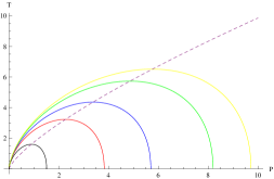
Figure 2: The isenthalpic curves. The mass are $1.4,1.8,2,2.2,2.3$ from inner to outer plots. We set $q=5$ and $\beta=2$.

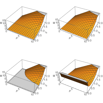
Figure 3: Relations of mass, event horizon and pressure. The parameters are $\beta=q=0;\beta=5,q=0;\beta=10,q=0$ and $\beta=10,q=5$, respectively.

The previous studies can be generalized to the case in which the kinetic term for the scalar fields can have non-linear contributions. Such a case can be implemented by the so-called k-essence models ArmendarizPicon:1999rj , in which the mentioned kinetic term are generalized to be a function $P(\psi,(\partial\psi)^{2})$. A simple case contained on this setup is the one in which the scalar fields apart from the standard kinetic term possess a kinetic nonlinear contribution given by higher powers of the kinetic term. The action was studied in Baggioli:2014roa ; Cisterna:2017jmv and is given by

$$S=\frac{1}{16\pi}\int\sqrt{-g}\left(R-2\Lambda-\frac{1}{4}F_{\mu\nu}F^{\mu\nu}-\sum_{i=1}^{2}(X_{i}+\gamma X_{i}^{k})\right)d^{4}x\,,$$ (20)

where $X_{i}=\frac{1}{2}\nabla^{\mu}\psi_{i}\nabla_{\mu}\psi_{i}$ with $i=1,2$. $\psi_{i}$ are massless scalar field. The above action goes back to that for the minimally coupled Einstein-Maxwell-scalars gravity studied in Andrade:2013gsa just by setting $\gamma=0$. The exact black hole solution for this theory was found in Cisterna:2017jmv

$$ds^{2} = -f(r)dt^{2}+\frac{dr^{2}}{f(r)}+r^{2}(dx_{1}^{2}+dx_{2}^{2}),\,$$ (21)

$$f(r) = \frac{r^{2}}{l^{2}}-\frac{2m}{r}-\frac{\lambda^{2}}{2}+\gamma\frac{\lambda^{2k}}{2^{k}(2k-3)}r^{2(1-k)}+\frac{q^{2}}{r^{2}},$$ (22)

with unchanged matter fields respect to the previous analyzed solution

$$\psi_{1} = \beta x_{1},\ \psi_{2}=\beta x_{2}\ ,$$ (23)

$$A = \left(\rho_{0}-\frac{2q}{r}\right)dt\,.$$ (24)

The extended thermodynamics of the above solution was studied by us in Hu:2019wwn . The Hawking temperature and the entropy of this black hole are given by

$$T=\frac{f^{\prime}(r_{h})}{4\pi}=2Pr_{h}-\frac{q^{2}}{4\pi r_{h}^{3}}-\frac{\beta^{2}}{8\pi r_{h}}-\frac{\gamma 2^{-k-2}\beta^{2k}r_{h}^{1-2k}}{\pi},$$ (25)

$$S=\frac{r_{h}^{2}}{4}.$$ (26)

We see that the temperature is modified by $\gamma$ while the entropy is the same as (11). The mass of the black hole and the charge are connected with $m$ and $q$ by means of

$$M=\frac{1}{16\pi}\left(\frac{\gamma 2^{1-k}\beta^{2k}r_{h}^{2(1-k)+1}}{2k-3}+\frac{16}{3}\pi Pr_{h}^{3}+\frac{2q^{2}}{r_{h}}-\beta^{2}r_{h}\right),~{}~{}Q=\frac{q}{8\pi}$$ (27)

where we have used the definition of pressure. The mass is computed by means of the Euclidean approach, namely, the partition function for a thermodynamical ensemble is identified with the Euclidean path integral in the saddle point approximation around the classical Euclidean solution. The detailed computations are shown in detail in Cisterna:2017jmv where the explicit realization of the first law of black hole thermodynamic for all values of $k$ is shown .

The charge and the thermodynamical volume as the conjugation of the pressure are the same as (9) and (15), respectively.

In order to analyze quantitatively the effect of the k-essence contribution on the Joule-Thomson expansion we will consider the $k=2$ case. By following the same strategy followed previously we obtain that for the inverse curve the horizon should satisfy the equation

$$3\gamma\beta^{4}-32\pi r_{h}^{4}P_{i}+4\beta^{2}r_{h}^{2}+12q^{2}=0.$$ (28)

By allowing only positive values for $\gamma$, no phantom contributions, there is only one positive root for $r_{h}$

$$r_{h}=\frac{1}{4}\sqrt{\frac{\beta^{2}}{\pi P_{i}}+\frac{\sqrt{\beta^{4}+24\pi\beta^{4}\gamma P_{i}+96\pi q^{2}P_{i}}}{\pi P_{i}}}.$$ (29)

Then, our inversion temperature is related with the inverse pressure by

$$T_{i}=\frac{(\sqrt{\sqrt{24\pi P_{i}\left(\gamma\beta^{4}+4q^{2}\right)+\beta^{4}}+\beta^{2})P_{i}}\left(\beta^{4}+16\pi P_{i}\left(\beta^{4}\gamma+4q^{2}\right)+\beta^{2}\sqrt{\beta^{4}+24\pi P_{i}\left(\beta^{4}\gamma+4q^{2}\right)}\right)}{2\sqrt{\pi}\left(\beta^{2}+\sqrt{\beta^{4}+24\pi P_{i}\left(\beta^{4}\gamma+4q^{2}\right)}\right){}^{2}}.$$ (30)

The inverse curve for different values of the $\gamma$ coupling are shown in figure 4.

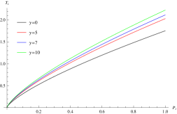
Figure 4: Inversion curves $T_{i}-P_{i}$ for heating and cooling processes for different values of $\gamma$. We set $q=5$ and $\beta=2$.

Similarly, the higher coupling also enhances the inverse curve.

Now we analyze the case in which $\gamma$ can take negative values. When considering this phantom contribution equation (28) possesses two positive roots defined by

$$r_{h_{-}}=\frac{1}{4}\sqrt{\frac{\beta^{2}}{\pi P_{i}}-\frac{\sqrt{\beta^{4}+24\pi\beta^{4}\gamma P_{i}+96\pi q^{2}P_{i}}}{\pi P_{i}}},~{}r_{h_{+}}=\frac{1}{4}\sqrt{\frac{\beta^{2}}{\pi P_{i}}+\frac{\sqrt{\beta^{4}+24\pi\beta^{4}\gamma P_{i}+96\pi q^{2}P_{i}}}{\pi P_{i}}}.$$ (31)

It is straightforward to compute when $-\frac{4q^{2}}{\beta^{4}}>\gamma>-\frac{1}{24\pi P_{i}}-\frac{4q^{2}}{\beta^{4}}$, both $r_{h_{-}}$ and $r_{h_{+}}$ are real positive roots, otherwise, only $r_{h_{+}}$ is positive. Substituting the two positive solution into the equation for $\mu_{JT}=0$, we can obtain two branches of the inversion curve. We show the possible positive root and the inversion curve with the related two branches in figure 5. However, with the same parameters, we found that the mass of black hole is negative for both $r_{h_{-}}$ and $r_{h_{+}}$, which implies that in this case, the Joule-Thomson expansion breaks down for negative $\gamma$. This is reasonable because negative $\gamma$ involves instability.

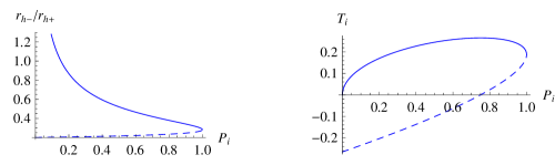
Figure 5: Left: The possible positive horizon VS the inversion pressure. Right: Inversion curves $T_{i}-P_{i}$ for heating and cooling processes for $\gamma=-\frac{25}{4}-\frac{1}{24\pi}$. We set $q=5$ and $\beta=2$.

III Joule-Thomson expansion in massive gravity

III.1 Planar black holes in massive gravity

Now we turn to the study of the Joule-Thomson expansion in the context of a massive gravity theory. We shall focus on four dimensional black holes with planar horizon. The action of the four-dimensional massive gravity we are considering is given by Vegh:2013sk

$$S=\frac{1}{16\pi}\int d^{4}x\sqrt{-g}\Big{[}R+\frac{6}{l^{2}}-\frac{1}{4}F^{2}+m_{g}^{2}\sum_{i=1}^{4}c_{i}\mathscr{U}_{i}(g,f)\Big{]},$$ (32)

where $m_{g}$ is the parameter controlling the massive term. We know that the presence of impurities in realistic materials involves that momentum is not conserved which brings in finite DC conductivity. Modeling systems with the use of translationally invariant quantum field theories always have problems unless the effects of momentum dissipation are incorporated. Fortunately, in the framework of holography, several methods employed to include momentum dissipation and extract the DC conductivity have been proposed. Massive gravity with the action (32) proposed by Vegh Vegh:2013sk is an alternative approach considering momentum dissipation holographically which provides an effective bulk description of a theory that does not conserve momentum without using any specific mechanism. In the action, in contrast with Einstein gravity, the last terms represent massive potentials associated with the graviton mass which breaks the diffeomorphism invariance in the bulk producing momentum relaxation in the dual boundary theory. The study of ghost-free massive gravity can be seen in Hassan:2011hr ; Hassan:2011tf .

In the action (32), The couplings $c_{i}$ are series of constants with dimension while $f$ and $\mathscr{U}_{i}$ denote the reference metric and symmetric polynomials of the eigenvalue of the ($4$)$\times$($4$) matrix $\mathscr{K}^{\mu}_{~{}\nu}\equiv\sqrt{g^{\mu\alpha}f_{\alpha\nu}}$, respectively. $\mathscr{U}_{i}$ have the forms

$$\mathscr{U}_{1} = [\mathscr{K}],~{}~{}~{}\mathscr{U}_{2}=[\mathscr{K}]^{2}-[\mathscr{K}^{2}],$$

$$\mathscr{U}_{3} = [\mathscr{K}]^{3}-3[\mathscr{K}][\mathscr{K}^{2}]+2[\mathscr{K}^{3}],$$

$$\mathscr{U}_{4} = [\mathscr{K}]^{4}-6[\mathscr{K}^{2}][\mathscr{K}]^{2}+8[\mathscr{K}^{3}][\mathscr{K}]+3[\mathscr{K}^{2}]^{2}-6[\mathscr{K}^{4}]$$ (33)

where $[\mathscr{K}]=\mathscr{K}^{\mu}_{~{}\mu}$ and the square root in $\mathscr{K}$ can be interpreted as $(\sqrt{\mathscr{K}})^{\mu}_{~{}\nu}(\sqrt{\mathscr{K}})^{\nu}_{~{}\lambda}=\mathscr{K}^{\mu}_{~{}\nu}$. It is noted that even though self-consistent massive gravity theory may require $c_{i}$ to be negative if $m_{g}^{2}>0$, the stability of fluctuations of fields deserves further analysis because the fluctuations of some fields with negative mass square could still be stable if the mass square obeys their related Breitenlohner-Freedman boundsCai:2014znn . Thus, in order to see more possible effect of massive terms on the JT expansion, here we do not take care of the sign of $c_{i}$ and will consider both positive and negative values.

The static planar black hole solution of the above action yields Vegh:2013sk ; Cai:2014znn

$$ds^{2} = -f(r)dt^{2}+\frac{dr^{2}}{f(r)}+r^{2}(dx^{2}+dy^{2}),$$ (34)

$$f_{\mu\nu} = \mathrm{diag}(0,0,c_{0}^{2}h_{ij}),$$ (35)

with $\mathscr{U}_{1}=2c_{0}/r$, $\mathscr{U}_{2}=2c_{0}^{2}/r^{2}$, and $\mathscr{U}_{3}=\mathscr{U}_{4}=0$ and

$$f(r) = \frac{r^{2}}{l^{2}}-\frac{m}{r}+\frac{q^{2}}{r^{2}}+\frac{c_{0}c_{1}m_{g}^{2}}{2}r+c_{0}^{2}c_{2}m_{g}^{2}$$ (36)

$$= \frac{8\pi P}{3}r^{2}-\frac{m}{r}+\frac{q^{2}}{r^{2}}+\frac{c_{0}c_{1}m_{g}^{2}}{2}r+c_{0}^{2}c_{2}m_{g}^{2},$$

where in the second line, we have used the definition of pressure (12) and set the volume of two dimensional space to be $1$. The extended thermodynamics of massive gravity has been studied in Xu:2015rfa ; Zou:2017juz . The integral constant $m$ and $q$ are connected with the mass and charge of the black hole as $M=m/8\pi$ and $Q=q/8\pi$, respectively. Then the requirement of $f(r_{h})=0$ gives us

$$M = \frac{c_{0}c_{1}m_{g}^{2}r_{h}^{2}}{16\pi}+\frac{c_{0}^{2}c_{2}m_{g}^{2}r_{h}}{8\pi}+\frac{Pr_{h}^{3}}{3}+\frac{q^{2}}{8\pi r_{h}},$$ (37)

which is the mass of black hole connected with the energy density of thermodynamical system as shown in Blake:2013bqa . The Hawking temperature $T$, the entropy $S$, the thermodynamic volume $V$, and the electric potential $\Phi$ were derived as

$$T = \frac{1}{4\pi}f^{\prime}(r_{h})=\frac{c_{0}^{2}c_{2}m_{g}^{2}}{4\pi r_{h}}+\frac{c_{0}c_{1}m_{g}^{2}}{4\pi}+2Pr_{h}-\frac{q^{2}}{4\pi r_{h}^{3}},$$ (38)

$$S = \int_{0}^{r_{h}}\frac{1}{T}\left(\frac{\partial M}{\partial r}\right)_{Q,P,c_{i}}dr=\frac{r_{h}^{2}}{4},$$ (39)

$$V = \left(\frac{\partial M}{\partial P}\right)_{S,Q,c_{i}}=\frac{r_{h}^{3}}{3},$$ (40)

$$\Phi = \left(\frac{\partial M}{\partial Q}\right)_{S,P,c_{i}}=\frac{16\pi}{r_{h}}Q=\frac{2q}{r_{h}}.$$ (41)

We note that the formulas of the entropy and the thermodynamical volume are the same as those (11) and (15) in Einstein-Maxwell-scalar theory we showed in previous sections. By treating the coupling constants $c_{i}$ as thermodynamical variables, it is straightforward to obtain the generalized first law of the black hole in the extended phase spaceXu:2015rfa

$$\mathrm{d}H = TdS+VdP+\Phi dQ+\frac{c_{0}m_{g}^{2}r_{h}^{2}}{16\pi}dc_{1}+\frac{c_{0}^{2}m_{g}^{2}r_{h}}{8\pi}dc_{2}.$$ (42)

Then, we look at the scaling (i.e. the dimensions) of the various thermodynamical quantities, see for instance Kastor:2009wy . Here we have $M,Q\propto[Length]^{1},S\propto[Length]^{2},P\propto[Length]^{-2},c_{1}\propto[Length]^{-1}$ and $c_{2}\propto[Length]^{0}$, therefore the modified Smarr relation of the black hole is

$$1\cdot M=H = 2\cdot TS-2\cdot\left(\frac{\partial M}{\partial P}\right)P+1\cdot\left(\frac{\partial M}{\partial Q}\right)Q+(-1)\cdot\left(\frac{\partial M}{\partial c_{1}}\right)c_{1}+0\cdot\left(\frac{\partial M}{\partial c_{2}}\right)c_{2}$$ (43)

$$= 2TS-2VP+\Phi Q-\frac{c_{0}c_{1}m_{g}^{2}}{16\pi}r_{h}^{2},$$

where the term with $c_{2}$ does not contribute because the dimension is zero.

III.2 Joule-Thomson expansion

We continue to study the Joule-Thomson expansion in massive gravity. Using (4), we get the Joule-Thomson expansion coefficient in massive gravity

$$\mu_{JT}=-\frac{2r_{h}^{3}\left(8\pi Pr_{h}^{2}-12\pi Tr_{h}-c_{0}^{2}c_{2}m_{g}^{2}\right)+6q^{2}r_{h}}{3\left(r_{h}^{2}\left(8\pi Pr_{h}^{2}+c_{0}c_{1}m_{g}^{2}r_{h}-c_{0}^{2}c_{2}m_{g}^{2}\right)-q^{2}\right)}.$$ (44)

Using $\mu_{JT}=0$ we find the inversion temperature

$$T_{i}=\frac{8\pi P_{i}r_{h}^{4}-c_{0}^{2}c_{2}m_{g}^{2}r_{h}^{2}+3q^{2}}{12\pi r_{h}^{3}}.$$ (45)

Making use of the Hawking temperature, we obtain that for the inversion points, the horizon should satisfy the equation

$$8\pi P_{i}r_{h}^{4}+\frac{3}{2}c_{0}c_{1}m_{g}^{2}r_{h}^{3}+2c_{0}^{2}c_{2}m_{g}^{2}r_{h}^{2}-3q^{2}=0.$$ (46)

We can solve $r_{h}$ from the above equation and then substitute it into (45) to get the $T_{i}$ as a function of $P_{i}$. In what follows, we shall fix $c_{0}=1$ without loss of generality and mainly study the effects of $c_{1}$ and $c_{2}$.

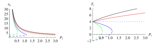
Figure 6: Left: Positive horizon $r_{h}$ for the inversion curve. Right: Inversion curves $T_{i}-P_{i}$ for heating and cooling processes for different values of the couplings. The upper plots are for $c_{1}=-1$ while the bottom plots are for $c_{1}=1$. Colors denote different $c_{2}$ with $c_{2}=2$ (green), $c_{2}=1$ (blue), $c_{2}=0$ (dashed), $c_{2}=-1$ (red) and $c_{2}=-2$ (black).

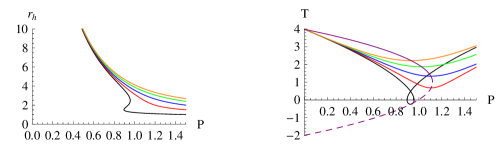
Figure 7: Left: The positive $r_{h}$ for the Isenthalpic curves for $c_{1}=-1$ and $c_{2}=1$. Right: Isenthalpic curves for heating and cooling processes for different values of the couplings.

We firstly consider the case with $q=0$. Consequently, beside $r_{h}=0$, there are two more solutions of (46) which are

$$r_{h}=\frac{\pm\sqrt{9c_{1}^{2}m_{g}^{4}-256\pi c_{2}m_{g}^{2}P_{i}}-3c_{1}m_{g}^{2}}{32\pi P_{i}}.$$ (47)

The inversion curves and the related horizon are shown in figure 6. In the upper plots, we set $c_{1}=-1$ to draw the positive $r_{h}$ (left) satisfying $\mu_{JT}=0$ and the related inversion curve (right). We observe two branches in the inversion curve for $c_{2}=2$ and $c_{2}=1$, and the related horizons are both positive. Furthermore, we study the isenthalpic curves for $c_{1}=-1$ and $c_{2}=1$ in the right plot of figure 7 where the purple line is the inversion curve. From the orange line to the black one, the mass of the black hole are $M=6,5,4,3.2$ and $2.5$ while the left plot is for the related horizon which are all positive. In the bottom plots, we draw the inversion curve for $c_{1}=1$ at the right side and at the left side we show the corresponding horizon. We see that for $c_{2}=2$ and $1$, even though there are two branches for the inversion curves, the horizons are all negative. So these cases are not physical and only the branches with $c_{2}=-2$ and $c_{1}=-1$ are physically significant.

These observations are novel in the following aspects. Comparing with previous works Okcu:2016tgt ; Ghaffarnejad:2018exz ; Mo:2018qkt ; Lan:2018nnp ; Okcu:2017qgo ; Mo:2018rgq ; Kuang:2018goo , where only one branch was obtained, we first obtain two branches for the inversion curve, which is similar to the Van der Waals fluids case. However, the minimal inversion temperature is negative unlike the case of Van der Waals fluids. On the other hand, for the isenthalpic curves in figure 7, the points $\mu_{JT}=(\partial T/\partial P)_{M}=0$ all fall in the inversion curve. However, we see here that $\mu_{JT}=0$ denotes the minimum but not maximal value which is a different behavior respect to the van der Waalss case and the other black hole cases that have been analyzed. This means that in the left side of the inversion curve, the isenthalpic process is a cooling process because of $\mu_{JT}<0$ while it is a warming process with $\mu_{JT}>0$ in the right side.

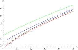
Figure 8: Inversion curves $P_{i}-T_{i}$ for heating and cooling processes with $c_{1}=1$. From bottom to up, $c_{2}$ are $(-4,-2,0,2,4)$.

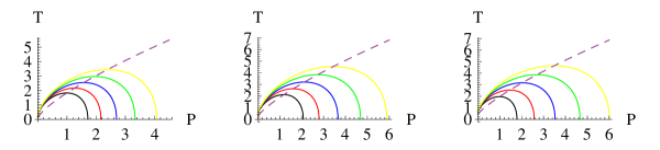
Figure 9: Isenthalpic curves for heating and cooling processes with $c_{2}=-2,2,4$.

We then consider the case with $q=5$. In this case, there are four solutions of equation (46) for $r_{h}$ , which we do not show due to esthetics purposes. We find with samples of $c_{1}$ and $c_{2}$, that only one solution is real and positive, therefore getting one branch for the inversion curve. We show the inversion curves with $c_{1}=1$ for different $c_{2}$ in figure 8, which is similar to the ones previously obtained in the literature with only one branch. Then the isenthalpic curves and the related inversion curves for choices of $c_{2}$ are shown in figure 9. Similarly, in each plot, the isenthalpic process in the left side of the inversion curve denotes warming process while those in the right side are for cooling process. Similar properties can be obtained for $c_{1}=-1$.

IV Final comments

By considering the cosmological constant as a thermodynamical quantity we have analyzed the Joule-Thomson expansion, this means, the expansion of gas from a higher pressure section to a lower one by maintaining the enthalpy of the process constant, this in the context of AdS planar black hole that exhibit momentum dissipation. Real materials relax momentum, behavior that from the point of view of gravitational dual theories, can be introduced by several methods that break translational invariance in the field theory side. Two methods were investigated, first when linear scalar fields, massless scalar fields that depend linearly on the horizon coordinates, are introduced, and secondly the case in which the Einstein-Hilbert action is supplemented with massive potentials that renders gravity massive and that break the bulk diffeomorphism invariance of the theory. By studying the Joule-Thomson coefficient, $\mu_{JT}$, which determines the transition from warming/cooling phases, we have computed the inversion curves in the $T_{i}-P_{i}$ plane as well as the corresponding isenthalpic curves.

We have observed that for the case of linear scalars, when they possess standard kinetic term, the inversion curve possesses only one branch, similar to what was obtained in Okcu:2016tgt ; Ghaffarnejad:2018exz ; Mo:2018qkt ; Lan:2018nnp ; Okcu:2017qgo ; Mo:2018rgq ; Kuang:2018goo , behavior that differs from the case of van der Waals fluids. The net effect of the momentum relaxation mechanism, which is controlled by our coupling $\beta$, is that the inversion curve is enlarged for higher values of $\beta$. This means that the temperature for which the heating/cooling transition takes place is greater when increasing $\beta$. In fact, the momentum relaxation parameter behave as an electric charge, not only enhancing the inversion curve, but also supporting the Joule-Thomson expansion in the absence of electric charge.

Next, we have modified the kinetic term for our scalars by including a nonlinear kinetic term of the type $(\partial_{\mu}\psi\partial^{\mu}\psi)^{k}$, contribution controlled by the parameter $\gamma$. We observe a similar behavior than in the previous case, this means, that considering greater values of $\gamma$ we obtain enlarged inversion curves. Nevertheless we observe (for the $k=2$ case) that allowing $\gamma$ to be negative, this means, by considering possible phantom contributions the inversion curve presents two branches. However, with the same parameters, the mass of black hole is negative which implies that in this case, the Joule-Thomson expansion breaks down for negative $\gamma$ because negative $\gamma$ involves instability.

For the case of the massive gravity theory we have found an interesting new behavior of the process, mostly related with the form of the isenthalpic curves. In the uncharged case, we observe that for some values of the relevant parameters we obtained two branches, but the related horizons and the temperature are all negative which are not physically significant. Nevertheless, when constructing the isenthlapic curves we observe that the inversion point represent a minimum of the isenthalpic curve instead of a maximum as it has been typically found Okcu:2016tgt ; Ghaffarnejad:2018exz ; Mo:2018qkt ; Lan:2018nnp ; Okcu:2017qgo ; Mo:2018rgq ; Kuang:2018goo . This implies that in the left side of the inversion curve, the isenthalpic process is a cooling process while it is a warming process in the right side. So far black holes where found to always cool when passing the inversion curve, nevertheless these solutions of massive gravity are able to heat when crossing it. The situation is restored to typical behaviors when including electric charge. We note that in the present work, we mainly focus on the possible features of the JT expansion. It would be very interesting to scan the values of parameters in accompany with the PV criticality Xu:2015rfa ; Zou:2017juz and further study the thermodynamical phenomenon in massive gravity. We will leave it for future work.

References

- (1) R. Ruffini and J. A. Wheeler, “Introducing the black hole,” Phys. Today 24, no. 1, 30 (1971).
- (2) J. D. Bekenstein, “Black holes: Classical properties, thermodynamics and heuristic quantization,” gr-qc/9808028.
- (3) J. D. Bekenstein, “Black holes and entropy”, Phys.Rev. D7 (1973) 2333-2346.
- (4) S. W. Hawking, “Particle Creation by Black Holes”, Commun. Math. Phys. 43 (1975) 199?220.
- (5) J. M. Bardeen, B. Carter and S. W. Hawking, “The Four laws of black hole mechanics”, Commun. Math. Phys. 31 (1973) 161-170.
- (6) J. M. Maldacena, “The large N limit of superconformal field theories and supergravity,” Adv. Theor. Math. Phys. 2 (1998) 231 [Int. J. Theor. Phys. 38 (1999) 1113].
- (7) S. W. Hawking and D. N. Page, “Thermodynamics of Black Holes in anti-De Sitter Space”, Commun. Math. Phys. 87 (1983) 577.
- (8) E. Witten, “Anti-de Sitter space and holography,” Adv. Theor. Math. Phys. 2, 253 (1998).
- (9) E. Witten, “Anti-de Sitter space, thermal phase transition, and confinement in gauge theories”, Adv. Theor. Math. Phys. 2 (1998) 505-532.
- (10) S. A. Hartnoll, P. K. Kovtun, M. Muller and S. Sachdev, “Theory of the Nernst effect near quantum phase transitions in condensed matter, and in dyonic black holes”, Phys. Rev. B76 (2007) 144502.
- (11) S. A. Hartnoll, C. P. Herzog and G. T. Horowitz, “Building a Holographic Superconductor”, Phys. Rev. Lett. 101 (2008) 031601.
- (12) S. B. Giddings, “The Black hole information paradox, in Particles, strings and cosmology”. Proceedings, 19th Johns Hopkins Workshop and 5th PASCOS Interdisciplinary Symposium, Baltimore, USA, March 22-25, 1995, pp. 415-428, 1995. hep-th/9508151.
- (13) P. Kovtun, D. T. Son and A. O. Starinets, “Viscosity in strongly interacting quantum field theories from black hole physics”, Phys. Rev. Lett. 94 (2005) 111601.
- (14) D. Kastor, S. Ray and J. Traschen, “Enthalpy and the Mechanics of AdS Black Holes,” Class. Quant. Grav. 26, 195011 (2009)
- (15) B. P. Dolan, “The cosmological constant and the black hole equation of state”, Class. Quant. Grav. 28 (2011) 125020.
- (16) M. Cvetic, G. W. Gibbons, D. Kubiznak and C. N. Pope, “Black Hole Enthalpy and an Entropy Inequality for the Thermodynamic Volume”, Phys. Rev. D84 (2011) 024037.
- (17) B. P. Dolan, D. Kastor, D. Kubiznak, R. B. Mann and J. Traschen, “Thermodynamic Volumes and Isoperimetric Inequalities for de Sitter Black Holes”, Phys. Rev. D87 (2013) 104017.
- (18) R.A. Hennigar, D. Kubiznak and R.B. Mann, “Entropy inequality violations from ul- traspinning black holes”, Phys. Rev. Lett. 115, no. 3, 031101 (2015).
- (19) R.A. Hennigar, D. Kubiznak, R.B. Mann and N. Musoke, “Ultraspinning limits and super-entropic black holes”, JHEP 1506, 096 (2015).
- (20) R.A. Hennigar and R.B. Mann, “Black holes in Einsteinian cubic gravity”, Phys. Rev. D 95, no. 6, 064055 (2017).
- (21) P. Bueno and P.A. Cano, “Einsteinian cubic gravity”, Phys. Rev. D 94, no. 10, 104005 (2016).
- (22) X. H. Feng, H. S. Liu, W. T. Lu and H. Lu, “Horndeski Gravity and the Violation of Reverse Isoperimetric Inequality,” Eur. Phys. J. C 77, no. 11, 790 (2017).
- (23) B. P. Dolan, “Where Is the PdV in the First Law of Black Hole Thermodynamics?,” arXiv:1209.1272 [gr-qc].
- (24) D. Kubiznak and R. B. Mann, “Black hole chemistry”, Can. J. Phys. 93 (2015) 999-1002.
- (25) R. B. Mann, “The Chemistry of Black Holes”, Springer Proc. Phys. 170 (2016) 197-205.
- (26) D. Kubiznak, R. B. Mann and M. Teo, “Black hole chemistry: thermodynamics with Lambda,” Class. Quant. Grav. 34, no. 6, 063001 (2017).
- (27) C. V. Johnson, “Holographic Heat Engines,” Class. Quant. Grav. 31, 205002 (2014).
- (28) R. A. Hennigar, F. McCarthy, A. Ballon and R. B. Mann, “Holographic heat engines: general considerations and rotating black holes,” Class. Quant. Grav. 34, no. 17, 175005 (2017).
- (29) L. Q. Fang and X. M. Kuang, “Holographic heat engine with momentum relaxation,” Sci. China Phys. Mech. Astron. 61, 080421 (2018).
- (30) S. Q. Hu and X. M. Kuang, “Holographic heat engine in Horndeski model with the -essence sector,” Sci. China Phys. Mech. Astron. 62 (2019) no.6, 60411.
- (31) F. Reif, “Fundamentals of Statistical and Thermal Physics” McGraw-Hill, New York, 1965.
- (32) Ö. Ökcü and E. Aydıner, “Joule-Thomson expansion of the charged AdS black holes,” Eur. Phys. J. C 77, no. 1, 24 (2017).
- (33) H. Ghaffarnejad, E. Yaraie and M. Farsam, Int. J. Theor. Phys. 57, no. 6, 1671 (2018).
- (34) J. X. Mo, G. Q. Li, S. Q. Lan and X. B. Xu, “Joule-Thomson expansion of -dimensional charged AdS black holes,” Phys. Rev. D 98 (2018) no.12, 124032.
- (35) Ö. Ökcü and E. Aydıner, “Joule-Thomson expansion of Kerr-AdS black holes,” Eur. Phys. J. C 78, no. 2, 123 (2018).
- (36) Z. W. Zhao, Y. H. Xiu and N. Li, “Throttling process of the Kerr-Newman-anti-de Sitter black holes in the extended phase space,” Phys. Rev. D 98 (2018) no.12, 124003.
- (37) S. Q. Lan, “Joule-Thomson expansion of charged Gauss-Bonnet black holes in AdS space,” Phys. Rev. D 98, no. 8, 084014 (2018).
- (38) J. X. Mo and G. Q. Li, “Effects of Lovelock gravity on the Joule-Thomson expansion,” arXiv:1805.04327 [gr-qc].
- (39) X. M. Kuang, B. Liu and A. Ovgun, “Novel nonlinear electrodynamics black hole and related phenomena in the extended thermodynamics,” Eur. Phys. J. C (2018) 78: 840.
- (40) T. Andrade and B. Withers, “A simple holographic model of momentum relaxation,” JHEP 1405, 101 (2014).
- (41) D. Vegh, “Holography without translational symmetry,” arXiv:1301.0537 [hep-th].
- (42) M. Baggioli and O. Pujolas, “Electron-Phonon Interactions, Metal-Insulator Transitions, and Holographic Massive Gravity,” Phys. Rev. Lett. 114, no. 25, 251602 (2015)
- (43) A. Cisterna, M. Hassaine, J. Oliva and M. Rinaldi, “Axionic black branes in the k-essence sector of the Horndeski model,” Phys. Rev. D 96, no. 12, 124033 (2017).
- (44) Y. Bardoux, M. M. Caldarelli and C. Charmousis, “Shaping black holes with free fields,” JHEP 1205, 054 (2012).
- (45) X. M. Kuang and J. P. Wu, “Thermal transport and quasi-normal modes in Gauss-Bonnet-axions theory,” Phys. Lett. B 770 (2017) 117.
- (46) A. Cisterna, C. Erices, X. M. Kuang and M. Rinaldi, “Axionic black branes with conformal coupling,” Phys. Rev. D 97 (2018) no.12, 124052.
- (47) A. Cisterna and J. Oliva, “Exact black strings and p-branes in general relativity,” Class. Quant. Grav. 35, no. 3, 035012 (2018).
- (48) G. W. Gibbons, R. Kallosh and B. Kol, “Moduli, scalar charges, and the first law of black hole thermodynamics,” Phys. Rev. Lett. 77, 4992 (1996) [hep-th/9607108].
- (49) D. Astefanesei, R. Ballesteros, D. Choque and R. Rojas, “Scalar charges and the first law of black hole thermodynamics,” Phys. Lett. B 782, 47 (2018).
- (50) M. Henneaux and C. Teitelboim, “The Cosmological Constant As A Canonical Variable,” Phys. Lett. 143B, 415 (1984).
- (51) C. Armendariz-Picon, T. Damour and V. F. Mukhanov, “k - inflation,” Phys. Lett. B 458, 209 (1999).
- (52) S. F. Hassan and R. A. Rosen, “Resolving the Ghost Problem in non-Linear Massive Gravity,” Phys. Rev. Lett. 108 (2012) 041101.
- (53) S. F. Hassan, R. A. Rosen and A. Schmidt-May, “Ghost-free Massive Gravity with a General Reference Metric,” JHEP 1202, 026 (2012).
- (54) R. G. Cai, Y. P. Hu, Q. Y. Pan and Y. L. Zhang, “Thermodynamics of Black Holes in Massive Gravity,” Phys. Rev. D 91, no. 2, 024032 (2015).
- (55) M. Blake and D. Tong, “Universal Resistivity from Holographic Massive Gravity,” Phys. Rev. D 88, no. 10, 106004 (2013).
- (56) E. Kiritsis, “Product CFTs, gravitational cloning, massive gravitons and the space of gravitational duals,” JHEP 0611, 049 (2006).
- (57) O. Aharony, A. B. Clark and A. Karch, “The CFT/AdS correspondence, massive gravitons and a connectivity index conjecture,” Phys. Rev. D 74, 086006 (2006).
- (58) L. Apolo and M. Porrati, “On AdS/CFT without Massless Gravitons,” Phys. Lett. B 714, 309 (2012).
- (59) J. Xu, L. M. Cao and Y. P. Hu, “P-V criticality in the extended phase space of black holes in massive gravity,” Phys. Rev. D 91, no. 12, 124033 (2015).
- (60) D. C. Zou, Y. Liu and R. H. Yue, “Behavior of quasinormal modes and Van der Waals-like phase transition of charged AdS black holes in massive gravity,” Eur. Phys. J. C 77, no. 6, 365 (2017).