Diffraction by a quarter–plane. Analytical continuation of spectral functions

Abstract

The problem of diffraction by a Dirichlet quarter-plane (a flat cone) in a 3D space is studied. The Wiener–Hopf equation for this case is derived and involves two unknown (spectral) functions depending on two complex variables. The aim of the present work is to build an analytical continuation of these functions onto a well-described Riemann manifold and to study their behaviour and singularities on this manifold. In order to do so, integral formulae for analytical continuation of the spectral functions are derived and used. It is shown that the Wiener–Hopf problem can be reformulated using the concept of additive crossing of branch lines introduced in the paper. Both the integral formulae and the additive crossing reformulation are novel and represent the main results of this work.

1 Introduction and literature review

Towards a generalisation of Sommerfeld’s solution.

In the late 19th century, Sommerfeld [1] published a solution to the problem of diffraction by a half-plane by reducing it to a two-dimensional problem and using a technique now known as Sommerfeld integrals (see e.g. [2]). Since, in particular thanks to Jones’ simplification [3], another popular way of solving this canonical problem is to make use of the Wiener-Hopf technique [4, 5, 6], which relies heavily on the concept of analytical continuation in one complex variable, as well as on the use of Liouville’s theorem. Knowledge of this canonical solution (among others) inspired the idea of (GTD) Geometrical Theory of Diffraction [7, 8]. The aim of the GTD is to describe the far-field resulting from diffraction by an obstacle exhibiting geometrical singularities such as edges or corners. In particular, the Sommerfeld solution allows an analytical description of the far-field diffracted by an edge.

Sommerfeld’s solution admits a direct generalisation to the case of diffraction by a wedge with scalar equation of motion, and so does the Wiener–Hopf solution [9, 10, 11].

In the mathematical sense, the Sommerfeld problem is that of diffraction by a half-line in a 2D medium. One can have a seemingly natural idea to generalize the Sommerfeld or the Wiener–Hopf method to the 3D space $(x_{1},x_{2},x_{3})$, in which the scatterer is a quarter-plane (a flat cone) placed at $x_{3}=0$, $x_{1}>0$, $x_{2}>0$. The quarter-plane may be hard (resp. soft) in the acoustic formulation, i.e. bear Neumann (resp. Dirichlet) boundary conditions on both faces. Surprisingly, this has proven to be a much more complicated problem, and, though there exists a simple to use closed-form solution of the half-plane problem, this is not yet the case for the quarter-plane. Such a problem can be treated as a canonical diffraction problem, and its solution would extend the applicability of the composite diffraction methods based on the locality principles, such as GTD or PTD (physical theory of diffraction). This problem is the subject of the present paper.

The quarter-plane as a flat cone.

The most classic approach (see [12]) uses the observation that a quarter-plane is a degenerate elliptic cone. Thus, it is possible to use separation of variables and sphero-conal coordinates in order to express the solution as a multipole series involving Lamé functions (see [13] for an in-depth description of these functions). However, the convergence of such series is very poor at high frequencies which made this approach difficult to use. A curious confirmation of the low usability of the series solution is the fact that URSI Commission B awarded a prize in 2005 for an accurate approximate solution of this problem. The winning approach, [14], was focused on enhancing convergence of the expansion series (see [15] and [16] for details). We should note here also an unusual work, [17], probably inspired by the URSI prize appeal, where the author make use of the Feynman-Kac theorem in order to express the corner-diffracted part of the field as a mean calculated from realisations of three simple stochastic differential equations.

An elegant approach applicable to diffraction by an arbitrary cone and particularly to a flat cone has been introduced in [18] and [19]. One converts the series into a contour integral by means of Bessel–Watson transform, and then deforms the contour to obtain fast convergence of the integral. The integrand contains a Green’s function for the Laplace-Beltrami operator on a sphere with a cut, which can be obtained, generally, by solving an integral equation. Within this approach, the concept of the oasis domain has been introduced, i.e. of the domain in the 3D space where there are no scattered waves except the spherical wave diffracted by the tip of the cone. The position of the observation point in the oasis guarantees fast convergence of the resulting integral for the diffraction coefficient. Outside the oasis, the field contains also some waves diffracted by the edges of the quarter-plane and some reflected waves, and the integral for the diffraction coefficient diverges. One can, however, regularize it by using Abel-Poisson type methods ([20], [21]).

Finding of the diffraction coefficient, i.e. the angular dependence of the diffracted spherical wave, is a complicated task, while other wave components can be found by relatively simple methods. An accurate description of such components can be given using GTD for example [22], Sommerfeld integrals [23, 24], or using ray asymptotics on a sphere with a cut [25]. An interesting link between the spherical diffracted wave and the other diffracted wave components can be found in [26]. It says that the diffraction coefficient of the spherical wave emanating from a corner can be written as the solution of a PDE in a unit ball, for which the boundary data on the surface is provided by the other wave components, which can be found explicitly.

The idea of a sphere with a cut arises from separation of variables in spherical coordinates. In particular, such approach (see for example [27]) allows one to describe the asymptotic behaviour of the solution in the near-field, close to the corner. The field behaves like $r^{\nu_{1}-1/2}$, where $r$ is the distance to the corner and $\nu_{1}=\sqrt{\lambda_{1}+1/4}$, where $\lambda_{1}$ is the first eigenvalue of the Laplace-Beltrami operator on the sphere with a cut. The spectral analysis of such operator is in itself a very interesting topic (see for example [28, 29] as well as [30] and references therein).

Building on the ideas of [18] and the concept of embedding formulae (introduced in [31] and developed further in [32]) and edge Green’s functions, more formulae, coined modified Smyshlyaev formulae, were introduced (see [33, 34, 35, 36, 37]) and showed to be naturally convergent in a region much larger than the oasis zone, which makes it one of the most successful current techniques. In fact this zone of convergence is the zone where no secondary diffracted wave is present in the far-field. This allowed for a fast computation of the diffraction coefficient for a wide range of incidence and observation directions in the case of Dirichlet and Neumann boundary conditions. Still, computation of the diffraction coefficient in the areas where doubly diffracted waves exist remains problematic and no methods have so far succeeded in doing so.

Generalisations of the Wiener–Hopf method.

The idea of generalisation of the usual (1D) Wiener–Hopf method seems attractive but is far from trivial and, as we believe, a proper generalisation demands development of substantially new methods. A “safe” approach, however, is described in [38], where the 1D Wiener–Hopf method is applied successively to different coordinates, and the resulting solution becomes expressed as a result of infinite number of such operations.

The difficulty with the 2D Wiener–Hopf method is as follows. In the 1D case, the Fourier transform of a function with a support on the positive half-axis $x$ is analytic in the upper half-plane of the Fourier variable $\xi$, and vice versa (see e.g. [6]). In the 2D case, a direct generalisation of this fact is valid, namely, a function having a support in the quadrant $x_{1}>0$, $x_{2}>0$, after a Fourier transform, gives a function analytic in the domain ${\rm Im}(\xi_{1})>0$, ${\rm Im}(\xi_{2})>0$ (see (2.7) for the definition of the Fourier transform and Theorem 2.3 for a rigorous statement of this result). The inverse statement is also true. The problem is that there exists no such a simple criterion for a function having its support in the complement of the quadrant, i.e. in $x_{1}<0$ or $x_{2}<0$. This problem does not arise in the 1D case since a complement of a half-line is also a half-line.

Some generalisations of the Wiener–Hopf method can be built if the kernel has special properties. Namely, if the kernel can be factorised into two kernels with supports in two quadrants, then the generalisation is straightforward [39, 40]. In [40] the restriction mentioned above has been slightly weakened to allow for kernels that can be written as a sum of two or three functions, the supports of which being restricted to a quadrant. Some special kernels (products of functions depending on a single variable) have been studied in [41]. Unfortunately, the kernel (2.9) to which the quarter-plane diffraction problem is reduced does not fit these restrictions. An attempt to factorise such a kernel was made in [42] and called wave factorisation, but we think that it is erroneous. The reason for this will be made much clearer in future work, when we will introduce the concept of bridges and arrows for surface of integration visualisation in $\mathbb{C}^{2}$.

It has to be mentioned that other attempts have been made and were somehow unsuccessful. One of the most famous such attempt is Radlow’s work ([43] and [44]) on an extension of the Wiener-Hopf technique to two complex variables, but his formal closed-form solution led to the wrong type of near-field behaviour and was hence considered erroneous by the community (see for example [45]). A formal description of where his proof went wrong (the solution does not satisfy the boundary condition) was given in [46], and, more recently, other technical reasons have been given in [47], showing along the way however that in the far-field and in the case of Dirichlet conditions, Radlow’s solution led to surprisingly accurate results.

To conclude this introduction, we can say that getting a closed-form solution of the quarter-plane diffraction problem is still a challenging theoretical and practical task. Particularly, a generalisation of the Wiener–Hopf method to the case of two complex variables would be a considerable achievement.

Aim of the paper.

The main aim of the present work, is to establish the theoretical framework needed to make progress with a two complex variables approach of the Wiener–Hopf technique. After deriving the functional equation associated to the quarter-plane problem, containing two unknown functions $\tilde{W}$ and $\tilde{U}^{\prime}$ of two complex variables, we will endeavour to explicitly exhibit domains where these functions can be analytically continued. This is motivated by the fact that, as illustrated in section 3.1, a remarkable characteristic of a usual 1D Wiener–Hopf equation is that such domains can be found without solving the problem explicitly. The ideas and methods introduced in this work can be applied to plane sectors with any interior angle (not just $\pi/2$), but the presence of many multiple edge diffractions would make the exposition quite cumbersome. The main results of this work are:

• the analytical continuation integral formulae given in Theorems 3.1 and 3.6, allowing to find the domain of analyticity of the spectral functions as given in Theorems 3.3, 3.5 and 3.8;

• the reformulation of the spectral problem given in Section 4.4 using the novel concept of additive crossing of branches defined in Definition 4.1.

In the future, though not in the present paper, we will show how the additive crossing property will lead naturally to the appearance of a $r^{\nu_{1}-1/2}$ behaviour at the corner. Moreover, the knowledge of the expected singularities on the whole of the Riemann manifold will help us to construct an approximation solution, not dissimilar to Radlow’s ansatz, but hopefully more accurate.

Plan of the paper.

In Section 2, we will derive the functional equation using Green’s theorem, which is a different approach to that used in [47] for example, and we will introduce the concept of 1/4-based and 3/4-based functions, allowing for a concise spectral formulation of the physical problem. In Section 3, we will show that the unknown functions of the functional equation can be analytically continued in some larger domains, the union of which constitute the whole of $\mathbbm{C}^{2}$ except some cuts. This task will be based on the use of explicit analytical continuation integral formulae. In Section 4.2, we will show that the unknown function $\tilde{U}^{\prime}$ has a very particular behaviour about two of its branch sets. We call this behaviour additive crossing and this allows us to rewrite the spectral formulation in a very different way to that of Section 2, which we will use in further work in order to derive specific results.

2 The quarter-plane functional problem

2.1 Formulation of the physical problem

Consider a 3D space $(x_{1},x_{2},x_{3})$ The scatterer is a quarter-plane (QP hereafter) $x_{3}=0$, $x_{1}>0$, $x_{2}>0$, as shown in Fig. 2.1 (left). Everywhere outside the scatterer the Helmholtz equation is valid for the total field:

$$\Delta u^{\rm t}+k^{2}u^{\rm t}=0,$$ (2.1)

where $k$ is a wavenumber parameter, such that $k^{2}=1+i\epsilon$, $\epsilon$ being a small positive parameter. The total field is the sum of the incident and scattered fields:

$$u^{\rm t}=u^{\rm in}+u.$$

The incident field is a plane wave given by

$$u^{\rm in}=\exp\left\{i\left(k_{1}x_{1}+k_{2}x_{2}-\sqrt{k^{2}-k_{1}^{2}-k_{2}^{2}}\,x_{3}\right)\right\}.$$

The boundary condition is of inhomogeneous Dirichlet type on both faces of the QP:

$$u(x_{1},x_{2},0)=-\exp\{i(k_{1}x_{1}+k_{2}x_{2})\}\qquad\text{ if }x_{1}>0\text{ and }\ x_{2}>0.$$ (2.2)

We assume that ${\rm Re}(k_{1})>0$, ${\rm Re}(k_{2})>0$, and both values have a small positive imaginary part. The condition ${\rm Re}(k_{1})>0$, ${\rm Re}(k_{2})>0$ is rather restrictive, since it means that the incident wave cannot produce a doubly diffracted wave. However in this paper, we only have the ambition to introduce the theoretical framework that will allow us to make progress. The extension of this work to all possible incidence directions will be the topic of future work.

The scattered field $u$ should also obey some radiation conditions at infinity in the limiting absorption form, that is, in the case of $\epsilon>0$, we need to have $u$ tends to $0$ as $r=(x_{1}^{2}+x_{2}^{2}+x_{3}^{2})^{1/2}$ tends to $\infty$.

Considering the symmetry of the problem allows us to reduce in a standard way the problem for the scattered field to a boundary value problem in the half space with mixed boundary condition. Here in particular, we find that the scattered field is symmetric and hence we can reduce the problem to $x_{1,2}\in\mathbb{R}$ and $x_{3}\in\mathbb{R}^{+}$, subject to the Neumann boundary condition

$$\frac{\partial u}{\partial x_{3}}(x_{1},x_{2},0)=0\quad\text{ if }\quad x_{1}<0\text{ or }x_{2}<0.$$ (2.3)

Hence, in terms of regularity, we just need $u$ to be infinitely smooth for $x_{3}>0$ and continuous as $x_{3}\rightarrow 0^{+}$. For the problem to be well posed, we also need to impose the so called Meixner conditions, or edge conditions stipulating that close to the edges, the field should decay like the square root of the distance to the edge. Hence there must exist two “edge functions” $e_{1}$ and $e_{2}$ such that

$$\left|u^{\rm t}(x_{1},x_{2},x_{3})\right|<e_{1}(x_{1})(x_{2}^{2}+x_{3}^{2})^{1/4}\text{ as }(x_{2}^{2}+x_{3}^{2})^{1/2}\rightarrow 0\text{ for a fixed }x_{1}>0,$$ (2.4)

$$\left|u^{\rm t}(x_{1},x_{2},x_{3})\right|<e_{2}(x_{2})(x_{1}^{2}+x_{3}^{2})^{1/4}\text{ as }(x_{1}^{2}+x_{3}^{2})^{1/2}\rightarrow 0\text{ for a fixed }x_{2}>0,$$ (2.5)

There is another Meixner condition that should be imposed at the vertex. There should exist a “corner function” $c$ such that

$$\left|u^{\rm t}(x_{1},x_{2},x_{3})\right|<c(\theta,\varphi)r^{\lambda}\text{ as }r\rightarrow 0\text{ for some }\lambda>-1/2,$$ (2.6)

where $(r,\theta,\varphi)$ are the usual spherical coordinates, $\theta$ and $\varphi$ being the polar and azimuthal angles respectively. A function $u$ that satisfies (2.1)–(2.6) and the radiation condition will be called a solution to the quarter-plane problem with a plane wave incidence.

2.2 Derivation of the functional equation

For any function $\phi(x_{1},x_{2},x_{3})$, define its double Fourier transform $\mathfrak{F}[\phi]$ by

$$\mathfrak{F}[\phi](\xi_{1},\xi_{2},x_{3}) = \int_{-\infty}^{\infty}\int_{-\infty}^{\infty}\phi(x_{1},x_{2},x_{3})e^{i(\xi_{1}x_{1}+\xi_{2}x_{2})}\,\mathrm{d}x_{1}\mathrm{d}x_{2}.$$ (2.7)

Subsequently, for any function $\tilde{\Phi}(\xi_{1},\xi_{2})$, we define its inverse Fourier transform $\mathfrak{F}^{-1}[\tilde{\Phi}]$ by

$$\mathfrak{F}^{-1}\left[\tilde{\Phi}\right](x_{1},x_{2}) = \frac{1}{4\pi^{2}}\int_{-\infty}^{\infty}\int_{-\infty}^{\infty}\tilde{\Phi}(\xi_{1},\xi_{2})e^{-i(\xi_{1}x_{1}+\xi_{2}x_{2})}\,\mathrm{d}\xi_{1}\mathrm{d}\xi_{2}.$$ (2.8)

Define also the kernel function $\tilde{K}$ by

$$\tilde{K}(\xi_{1},\xi_{2})\equiv(k^{2}-\xi_{1}^{2}-\xi_{2}^{2})^{-1/2}.$$ (2.9)

For real $\xi_{1}$, $\xi_{2}$ such that $\xi_{1}^{2}+\xi_{2}^{2}<1$ the square root value is taken to be close to real positive.

Consider the domain $\Omega_{R,\varepsilon}$ consisting of the upper hemisphere of radius $R>0$ centred at the vertex, from which a sphere of radius $\varepsilon>0$ (around the vertex) has been removed. Hence the boundary of $\Omega_{R,\varepsilon}$ consists of the upper surface of the big sphere $S_{R}^{+}$ and a “bottom lid” made of two planar, and one spherical surfaces as shown in Fig. 2.1 (centre).

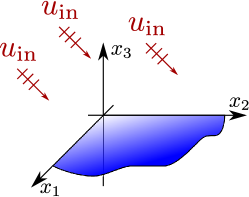
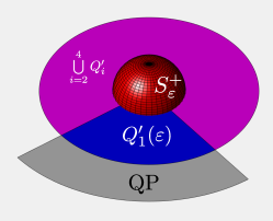
Figure 2.1: (left) Geometry of the problem. (centre) “Bottom lid” of $\Omega_{R,\varepsilon}$. The quarter-plane is in grey. (right) Illustration of the $Q_{i}$ quadrants.

For any test function $w$ that satisfies the Helmholtz equation, we can take the volume integral over $\Omega_{R,\varepsilon}$ of the quantity $w\Delta u-u\Delta w$. On one hand it is zero because of the Helmholtz equation, and on the other hand this can be expressed as a surface integral over $\partial\Omega_{R,\varepsilon}$ by Green’s theorem. Hence we get

$$\iint_{\partial\Omega_{R,\varepsilon}}\left(w\frac{\partial u}{\partial n}-u\frac{\partial w}{\partial n}\right)\,\mathrm{d}S = 0,$$ (2.10)

for any $\varepsilon>0$, where $\partial/\partial n$ is the normal derivative, where the unit normal ${\bf n}$ is chosen to be incoming towards the volume $\Omega_{R,\varepsilon}$, and the test function $w$ is chosen to be

$$w = e^{i(\xi_{1}x_{1}+\xi_{2}x_{2}+x_{3}/\tilde{K}(\xi_{1},\xi_{2}))},$$ (2.11)

for some $\xi_{1}$ and $\xi_{2}$. First, we take real $\xi_{1}$ and $\xi_{2}$ and then continue the results analytically. Note that for all real $\xi_{1}$, $\xi_{2}$ the value $\tilde{K}^{-1}(\xi_{1},\xi_{2})$ has a positive imaginary part. It is small (due to $\epsilon$) for $\xi_{1}^{2}+\xi_{2}^{2}<1$, and not small for $\xi_{1}^{2}+\xi_{2}^{2}>1$. Thus, $w$ decays exponentially as $x_{3}\to\infty$.

Note that there is no need to exclude the edges of the quarter-plane from our volume of integration since thanks to Meixner conditions the integrals are convergent there. Hence, thanks to the exponential decay of $w$, for any $\epsilon>0$, we have

$$\lim_{R\rightarrow\infty}\iint_{S_{R}^{+}}\left(w\frac{\partial u}{\partial n}-u\frac{\partial w}{\partial n}\right)\,\mathrm{d}S = 0.$$ (2.12)

Hence, if we call $Q_{i}^{\prime}(\varepsilon)$ the part of the quadrant $Q_{i}$ (see Figure 2.1) from which the disk of radius $\varepsilon$ is excluded, and $S_{\varepsilon}^{+}$ the upper small spherical surface around the vertex, taking the limit as $R\rightarrow\infty$ in (2.10), using the fact that ${\bf n}={\bf e}_{r}$ on $S_{\varepsilon}^{+}$ and ${\bf n}={\bf e}_{x_{3}}$ on $Q_{i}^{\prime}$ leads to

$$\iint_{S_{\varepsilon}^{+}}\left(w\frac{\partial u}{\partial r}-u\frac{\partial w}{\partial r}\right)\,\mathrm{d}S+\iint_{\bigcup\limits_{i=1}^{4}Q_{i}^{\prime}}\left(w\frac{\partial u}{\partial x_{3}}-u\frac{\partial w}{\partial x_{3}}\right)\,\mathrm{d}S = 0,$$ (2.13)

for any $\varepsilon>0$.

Due to the vertex Meixner condition, one can take the limit $\varepsilon\rightarrow 0$ in (2.13). As a result, the integral along $S_{\varepsilon}^{+}$ goes to zero. The integrals in the second term in the left of (2.13) become Fourier transforms of $u$ and $\partial u/\partial x_{3}$. Define

$$\tilde{U}(\xi_{1},\xi_{2})=\mathfrak{F}[u](\xi_{1},\xi_{2},0^{+}) \tilde{W}(\xi_{1},\xi_{2})=\mathfrak{F}\left[\frac{\partial u}{\partial x_{3}}\right](\xi_{1},\xi_{2},0^{+}).$$ and (2.14)

It follows from (2.13) that

$$\tilde{K}(\xi_{1},\xi_{2})\tilde{W}(\xi_{1},\xi_{2})=i\tilde{U}(\xi_{1},\xi_{2}),$$ (2.15)

which is the main functional equation for the QP diffraction problem. Indeed, this agrees with the functional equation from [43] and from other papers dedicated to the problem.

As it is, equation (2.15) is defined for real $\xi_{1},\xi_{2}$. The real plane $(\xi_{1},\xi_{2})$, on which $\tilde{U}$ and $\tilde{W}$ are defined by (2.14) is said to belong to the the “physical sheet”. Later on we will study analytical continuation of $\tilde{U}$ and $\tilde{W}$ to other “sheets”.

2.3 1/4-based and 3/4-based functions

Equation (2.15) contains two unknown functions. Our aim is to convert this equation into a formulation close to the traditional Wiener–Hopf equation. For this, we need to take into account some additional properties of the unknown functions $\tilde{U}$ and $\tilde{W}$. We call these properties 1/4-basedness and 3/4-basedness.

Define the quadrants $Q_{1},Q_{2},Q_{3},Q_{4}$ of the plane $(x_{1},x_{2})$ as it is shown in Fig. 2.1 (right). Now, upon writing $\boldsymbol{x}=(x_{1},x_{2})$ and $\boldsymbol{\xi}=(\xi_{1},\xi_{2})$, note that for any function $\phi(\boldsymbol{x})$, we can write $\mathfrak{F}[\phi]=\mathfrak{F}_{1/4}[\phi]+\mathfrak{F}_{3/4}[\phi]$, where the Fourier operators $\mathfrak{F}_{1/4}$ and $\mathfrak{F}_{3/4}$ are defined by

$$\mathfrak{F}_{1/4}[\phi](\boldsymbol{\xi})=\iint_{Q_{1}}\phi(\boldsymbol{x})e^{i\boldsymbol{x}\cdot\boldsymbol{\xi}}\,\mathrm{d}\boldsymbol{x} \mathfrak{F}_{3/4}[\phi](\boldsymbol{\xi})=\iint_{\bigcup\limits_{i=2}^{4}Q_{i}}\phi(\boldsymbol{x})e^{i\boldsymbol{x}\cdot\boldsymbol{\xi}}\,\mathrm{d}\boldsymbol{x},$$ and

and called $1/4$-range and $3/4$-range Fourier transform respectively. According to (2.3), the function $\tilde{W}$ is a Fourier transform of a function that is not equal to zero only on the quadrant $Q_{1}$. Similarly, according to (2.2), the function $\tilde{U}$ can be represented as follows:

$$\tilde{U}(\xi_{1},\xi_{2})=\frac{1}{(\xi_{1}+k_{1})(\xi_{2}+k_{2})}+\tilde{U}^{\prime}(\xi_{1},\xi_{2}).$$ (2.16)

The first term is the $\mathfrak{F}_{1/4}$ transform of (2.2), while $\tilde{U}^{\prime}$ is the $\mathfrak{F}_{3/4}$ transform of $u(x_{1},x_{2},0)$.

Definition 2.1.

A function $\tilde{\Phi}(\xi_{1},\xi_{2})$ is called 1/4-based if its inverse Fourier transform $\mathfrak{F}^{-1}[\tilde{\Phi}](x_{1},x_{2})$ is equal to zero if $x_{1}<0$ or $x_{2}<0$ (i.e. on quadrants $Q_{2},Q_{3},Q_{4}$). In other words, $\tilde{\Phi}$ is 1/4-based if there exists a function $\phi$ such that $\tilde{\Phi}=\mathfrak{F}_{1/4}[\phi]$.

Definition 2.2.

A function $\tilde{\Phi}(\xi_{1},\xi_{2})$ is called 3/4-based if its inverse Fourier transform $\mathfrak{F}^{-1}[\tilde{\Phi}](x_{1},x_{2})$ is equal to zero if $x_{1}>0$ and $x_{2}>0$ (i.e. on quadrant $Q_{1}$). In other words, $\tilde{\Phi}$ is 3/4-based if there exists a function $\phi$ such that $\tilde{\Phi}=\mathfrak{F}_{3/4}[\phi]$.

Thus, it is clear from the discussion above, that $\tilde{W}$ is 1/4-based and $\tilde{U}^{\prime}$ is 3/4-based. As discussed briefly in the introduction, the concept of a 1/4-based function causes no problem. Similarly to the 1D Wiener–Hopf method, one can formulate the following theorem.

Theorem 2.3.

Let us consider a function $\phi(x_{1},x_{2})$ having its Fourier transform equal to zero outside $Q_{1}$, and growing no faster than a polynomial for large $x_{1},x_{2}$. Then $\mathfrak{F}[\phi](\xi_{1},\xi_{2})$ can be analytically continued to the domain ${\rm Im}(\xi_{1})>0$, ${\rm Im}(\xi_{2})>0$ and has no singularities there. Reciprocally, if a function $\tilde{\Phi}(\xi_{1},\xi_{2})$ can be analytically continued to the domain ${\rm Im}(\xi_{1})>0$, ${\rm Im}(\xi_{2})>0$ and has no singularities there. Then $\tilde{\Phi}$ is 1/4-based.

Thus, there is a simple criterion of 1/4-basedness displayed in terms of analyticity. The known problems with building a 2D analog of the Wiener–Hopf method are connected with the concept of 3/4-basedness. Namely, there is no simple criterion of 3/4-basedness. An obvious statement that $\tilde{\Phi}(\xi_{1},\xi_{2})$ is 3/4-based if and only if it can be represented as

$$\tilde{\Phi}(\xi_{1},\xi_{2})=\tilde{\Phi}_{1}(-\xi_{1},\xi_{2})+\tilde{\Phi}_{2}(\xi_{1},-\xi_{2})+\tilde{\Phi}_{3}(-\xi_{1},-\xi_{2}),$$

where $\tilde{\Phi}_{1},\tilde{\Phi}_{2},\tilde{\Phi}_{3}$ are 1/4-based functions is not particularly useful on a practical level since it leads to the introduction of three unknown functions instead of one.

The present paper is an attempt to formulate a criterion of 3/4-basedness. We will show in Section 4 that it is connected with the idea of additive crossing of branch lines.

2.4 Formulation of the functional problem

Let us formulate the functional problem, i.e. the problem for the unknown function $\tilde{W}(\xi_{1},\xi_{2})$, which would be equivalent to the initial physical problem for $u(x_{1},x_{2},x_{3})$ given in Section 2.1. We assume that the functional equation (2.15) is valid, and, using (2.16), we define $\tilde{U}^{\prime}$ as follows

$$\tilde{U}^{\prime}(\xi_{1},\xi_{2})\equiv-i\tilde{K}(\xi_{1},\xi_{2})\,\tilde{W}(\xi_{1},\xi_{2})-\frac{1}{(\xi_{1}+k_{1})(\xi_{2}+k_{2})}.$$ (2.17)

The functional problem can be formulated in the form of the following theorem.

Theorem 2.4.

Let the function $\tilde{W}(\xi_{1},\xi_{2})$ have the following properties:

1. $\tilde{W}(\xi_{1},\xi_{2})$ is 1/4-based.

2. $\tilde{U}^{\prime}(\xi_{1},\xi_{2})$, as defined by (2.17), is 3/4-based.

3. There exist functions $E_{1}(\xi_{1})$ and $E_{2}(\xi_{2})$ defined for complex $\xi_{1}$ and $\xi_{2}$, such that

   $$|\tilde{W}(\xi_{1},\xi_{2})|<E_{1}(\xi_{1})|\xi_{2}|^{-1/2}\qquad\mbox{as}\quad|\xi_{2}|\rightarrow\infty,\quad{\rm Im}(\xi_{2})>0,$$ (2.18)

   $$|\tilde{W}(\xi_{1},\xi_{2})|<E_{2}(\xi_{2})|\xi_{1}|^{-1/2}\qquad\mbox{as}\quad|\xi_{1}|\rightarrow\infty,\quad{\rm Im}(\xi_{1})>0.$$ (2.19)

4. There exists a function $C(\beta,\psi_{1},\psi_{2})$ defined for $0<\beta<\pi/2$ and
   ${0<\psi_{1,2}<\pi}$ such that for real $\Lambda$

   $$|\tilde{W}(\xi_{1},\xi_{2})|<C(\beta,\psi_{1},\psi_{2})\Lambda^{-1-\lambda},\qquad\lambda>-1/2,$$ (2.20)

   where $\xi_{1}$ and $\xi_{2}$ are parametrised as follows for large real $\Lambda$:

   $$\xi_{1}=\Lambda e^{i\psi_{1}}\cos(\beta),\qquad\xi_{2}=\Lambda e^{i\psi_{2}}\sin(\beta),$$ (2.21)

Then the field $u(x_{1},x_{2},x_{3})$ defined by

$$u(x_{1},x_{2},x_{3})=-i\mathfrak{F}^{-1}[\tilde{K}\,\tilde{W}\,\exp\{i|x_{3}|/\tilde{K}\}](x_{1},x_{2}).$$ (2.22)

obeys all conditions of the initial physical problem and is hence a solution to the quarter-plane problem.

Proof.

The Ansatz (2.22) obeys (2.1) in $x_{3}\neq 0$ by construction. The radiation condition is fulfilled because of the imaginary part of $k$ and positive imaginary part of $\tilde{K}^{-1}$. The first condition of the theorem is responsible for the Neumann boundary condition (2.3) outside the QP. The second condition yields the Dirichlet boundary condition (2.2) on the QP. The third condition corresponds to the edge conditions (2.4) and (2.5). Obviously, the functions $E_{1}$ and $E_{2}$ are Fourier images of $e_{1}$ and $e_{2}$. Finally, the fourth condition provides the vertex condition (2.6). ∎

3 Analytical continuation of $\tilde{W}$

3.1 Motivation

We pay a considerable attention to the possibility of continuing the unknown function to some well-defined Riemann manifold. Though in the 1D case there is no clear path from the Riemann surface to the actual solution, on the intuitive level, we strongly believe that the possibility to solve the usual 1D Wiener–Hopf problem is linked with the possibility to study the analytical continuation of the unknown function without solving the problem. We illustrate below what we mean by this.

Consider a sample 1D problem of the form

$$K(\xi)\,W_{+}(\xi)+U_{-}(\xi)=T(\xi),$$ (3.1)

where $\xi$ is a scalar complex variable, $K(\xi)$ is a known coefficient, which is an algebraic function, $W_{+}$ and $U_{-}$ are unknown functions analytic in the upper and lower half-plane respectively and $T$ is a known right-hand side, which is a rational function. Equation (3.1) can be rewritten as

$$W_{+}(\xi)=K^{-1}(\xi)\,T(\xi)-K^{-1}(\xi)\,U_{-}(\xi)$$ (3.2)

and

$$U_{-}(\xi)=T(\xi)-K(\xi)\,W_{+}(\xi),$$ (3.3)

Note that $W_{+}$ is naturally defined in the upper half-plane, while the right-hand side of (3.2) is naturally defined in the lower half-plane. Thus, (3.2) can be used to continue $W_{+}$ into the lower half-plane. Similarly, (3.3) can be used to continue $U_{-}$ into the upper half-plane.

Let $W_{+}^{\star}(\xi)$ be the value of $W_{+}$ at some real $\xi$ of the “physical sheet”, i.e. the value that can be used for computation of some wave field. Similarly, let $U_{-}^{\star}(\xi)$ be the value of $U_{-}$ on the physical sheet.

Let us continue $W_{+}$ along some loop $\sigma$ starting and ending at $\xi$. The result will be denoted by $W_{+}(\xi;\sigma)$. Fix also the physical sheet of the argument of $K$ by $K^{\star}(\xi)$ and denote different branches of it by $K(\xi;\sigma)$.

Assume that $\sigma$ is homotopic to a concatenation of loops

$$\sigma=\sigma_{1}^{-}\sigma_{2}^{+}\sigma_{3}^{-}\dots$$

where the left loop is passed first, loops $\sigma_{j}^{+}$ are located in the upper half-plane, and $\sigma_{j}^{-}$ are located in the lower half-plane. See Fig. 3.1 for an illustration.

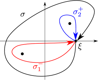
Figure 3.1: Illustration of a loop $\sigma$ homotopic to $\sigma_{1}^{-}\sigma_{2}^{+}$ in the case of a kernel $K$ with two branch points denoted by $\bullet$

It is hence possible to construct $W_{+}(\xi;\sigma)$ by iterations. First, use (3.2) for the loop $\sigma_{1}^{-}$ and get

$$W_{+}(\xi;\sigma_{1}^{-})=K^{-1}(\xi;\sigma_{1}^{-})\,T(\xi)-K^{-1}(\xi;\sigma_{1}^{-})\,U_{-}^{\star}(\xi).$$ (3.4)

Combining this with (3.3) obtain

$$W_{+}(\xi;\sigma_{1}^{-})=K^{-1}(\xi;\sigma_{1}^{-})\,K^{\star}(\xi)\,W_{+}^{\star}(\xi).$$ (3.5)

Continuing (3.5) along $\sigma_{2}^{+}$, obtain

$$W_{+}(\xi;\sigma_{1}^{-}\sigma_{2}^{+})=K^{-1}(\xi;\sigma_{1}^{-}\sigma_{2}^{+})\,K(\xi;\sigma_{2}^{+})\,W_{+}^{\star}(\xi).$$ (3.6)

This process can be continued, providing $W_{+}(\xi;\sigma_{1}^{-}\sigma_{2}^{+}\sigma_{3}^{-})$, $W_{+}(\xi;\sigma_{1}^{-}\sigma_{2}^{+}\sigma_{3}^{-}\sigma_{4}^{+})$, etc. At each step the value $W_{+}(\xi;\sigma)$ is $W_{+}^{\star}(\xi)$ multiplied by some values of $K$ and $K^{-1}$ on different branches.

Equations (3.4) and (3.6) are examples of analytical continuation formulae. These formulae provide information about the analytical structure of the function $W_{+}$ even without solving the Wiener–Hopf equation. Namely, one can reveal the structure of the Riemann surface of $W_{+}$ and find all singularities on this Riemann surface.

The aim of this section is to build formulae of analytical continuation for the 2D Wiener–Hopf problem formulated above. Unfortunately, in the 2D case such formulae are considerably more complicated, namely, they include integral operators. Still, they are helpful and provide an important information about 3/4-based functions.

3.2 Primary formulae for analytical continuation

The two unknown functions are, formally, $\tilde{W}$ and $\tilde{U}^{\prime}$. As we noted above, the natural domain of analyticity of the 1/4-based function $\tilde{W}(\xi_{1},\xi_{2})$ is ${\rm Im}(\xi_{1})>0$, ${\rm Im}(\xi_{2})>0$. In our consideration we use an important “physical” conjecture that the field has an exponential decay due to the presence of the imaginary part of $k$ corresponding to absorption in the medium. Namely, we estimate the field as

$$|u(x_{1},x_{2},0^{+})|<C_{\epsilon}\exp\{-4\kappa\sqrt{x_{1}^{2}+x_{2}^{2}}\}\quad\mbox{ as }\quad\sqrt{x_{1}^{2}+x_{2}^{2}}\to\infty$$ (3.7)

for

$$\kappa=\tfrac{1}{4}\,{\rm min}\,(\epsilon/2,{\rm Im}(k_{1}),{\rm Im}(k_{2})).$$

Thus, since $2\sqrt{x_{1}^{2}+x_{2}^{2}}>x_{1}+x_{2}$, one can easily prove that $\tilde{W}(\xi_{1},\xi_{2})$ is actually analytic in the wider domain

$${\rm Im}(\xi_{1})>-2\kappa,\qquad{\rm Im}(\xi_{2})>-2\kappa.$$

Note that nothing can be said a priori about the domain of analyticity of the second unknown function $\tilde{U}^{\prime}(\xi_{1},\xi_{2})$, which is 3/4-based.

Let us now introduce the important function $\gamma$ by

$$\gamma(\xi_{1},\xi_{2})\equiv\sqrt{\sqrt{k^{2}-\xi_{1}^{2}}+\xi_{2}},$$ (3.8)

for which the “arithmetic” branches of the square roots on the “physical sheet” are considered, i.e. the value of a square root for a real positive argument is positive real. Note that $\gamma$ participates in a multiplicative factorisation of $\tilde{K}$:

$$\tilde{K}(\xi_{1},\xi_{2})=\frac{1}{\gamma(\xi_{1},\xi_{2})\,\gamma(\xi_{1},-\xi_{2})}=\frac{1}{\gamma(\xi_{2},\xi_{1})\,\gamma(\xi_{2},-\xi_{1})}.$$ (3.9)

Using this function, we can formulate our first analytical continuation formulae.

Theorem 3.1.

For $|\textup{Im}(\xi_{1,2})|<\kappa$, $\tilde{W}$ obeys the following relations:

$$\tilde{W}(\xi_{1},\xi_{2}) = \frac{\gamma(\xi_{1},\xi_{2})}{4\pi^{2}}\!\!\!\!\!\int\limits_{-\infty-i\kappa}^{\infty-i\kappa}\!\!\!\!\!\!\mathrm{d}\xi_{2}^{\prime}\int\limits_{-\infty+i\kappa}^{\infty+i\kappa}\!\!\!\!\!\!\mathrm{d}\xi_{1}^{\prime}\,\frac{\gamma(\xi_{1},-\xi_{2}^{\prime})\,\tilde{K}(\xi_{1}^{\prime},\xi_{2}^{\prime})\,\tilde{W}(\xi_{1}^{\prime},\xi_{2}^{\prime})}{(\xi_{1}^{\prime}-\xi_{1})(\xi_{2}^{\prime}-\xi_{2})}$$ (3.10)

$$+ \frac{i\gamma(\xi_{1},\xi_{2})\,\gamma(\xi_{1},k_{2})}{(\xi_{1}+k_{1})(\xi_{2}+k_{2})}$$

$$\tilde{W}(\xi_{1},\xi_{2}) = \frac{\gamma(\xi_{2},\xi_{1})}{4\pi^{2}}\!\!\!\!\!\int\limits_{-\infty-i\kappa}^{\infty-i\kappa}\!\!\!\!\!\!\mathrm{d}\xi_{1}^{\prime}\int\limits_{-\infty+i\kappa}^{\infty+i\kappa}\!\!\!\!\!\!\mathrm{d}\xi_{2}^{\prime}\,\frac{\gamma(\xi_{2},-\xi_{1}^{\prime})\,\tilde{K}(\xi_{1}^{\prime},\xi_{2}^{\prime})\,\tilde{W}(\xi_{1}^{\prime},\xi_{2}^{\prime})}{(\xi_{1}^{\prime}-\xi_{1})(\xi_{2}^{\prime}-\xi_{2})}$$ (3.11)

$$+ \frac{i\gamma(\xi_{2},\xi_{1})\,\gamma(\xi_{2},k_{1})}{(\xi_{1}+k_{1})(\xi_{2}+k_{2})}.$$

The proof of this Theorem 3.1 is given in Appendix A. The relations (3.10) and (3.11) are integral equations for $\tilde{W}$, however, we will use them in another way, namely, for continuation of $\tilde{W}$ onto a Riemann manifold. Indeed, even if the right hand side of formulae (3.10) and (3.11) require $\tilde{W}$ to be known in a narrow strip near the real plane, one can choose $\xi_{1},\xi_{2}$ (the arguments of $\tilde{W}$ in the left hand side) to belong to a much wider domain, and, doing so, provide the required continuation. This will be explained in more detail below.

3.3 Domains for analytical continuation

Let us define the domains $H^{+}$ and $H^{-}$ as domains of a complex plane of a single variable, being the upper and the lower half-planes cut along the curves $h^{+}$ and $h^{-}$ (see Fig. 3.2, left). These curves are the sets of points

$$h^{\pm}:\quad\xi=\pm\sqrt{k^{2}-\tau^{2}},\quad\tau\in\mathbb{R}.$$

Let $\hat{H}^{+}$ be the upper half-plane, which is not cut along $h^{+}$. The domains in all cases are open, i.e. the boundary is not included. The boundary of $H^{-}$ consists of two parts: the real axis and the curve $h^{-}$ (passed two times, from $-i\infty$ to $-k$ along the right shore of the cut and backwards along the left shore of the cut). Denote this pass by $P$ (see Fig. 3.2, right), so the boundary of $H^{-}$ is $\partial H^{-}=\mathbb{R}\cup P$. Similarly, the boundary of $H^{+}$ is $\partial H^{+}=\mathbb{R}\cup(-P)$.

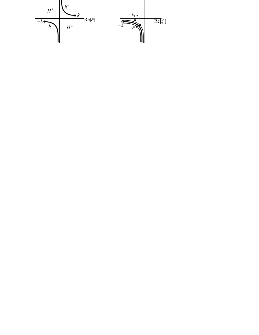
Figure 3.2: Domains $H^{\pm}$ (left), contour $P$, right

An important property of the domains $H^{\pm}$ is the following lemma.

Lemma 3.2.

Let the branch of the square root $\sqrt{k^{2}-\xi^{2}}$ be chosen such that this function have positive imaginary part for real $\xi$. If $\xi\in H^{+}$ or $\xi\in H^{-}$, then $\sqrt{k^{2}-\xi^{2}}\in H^{+}$.

Proof.

Let be $\xi\in H^{+}$. Consider the mapping $\xi\to\sqrt{k^{2}-\xi^{2}}$. This mappings maps the real axis onto $-P$, and $-P$ onto the real axis. Thus, according to the principles of conforming mapping, $H^{+}$ is mapped onto $H^{+}$.

Let now be $\xi\in H^{-}$. The real axis maps onto $-P$, and $P$ maps onto the real axis. Thus, $H^{-}$ is mapped onto $H^{+}$. ∎

3.4 First step of analytical continuation

Initially, as a 1/4-based function, $\tilde{W}(\xi_{1},\xi_{2})$ is analytic in the domain $\hat{H}^{+}\times\hat{H}^{+}$. It is easy to show that, besides, $\tilde{W}$ is continuous at the boundary of this domain (for example one can note, as it has been mentioned above, that $\tilde{W}$ is analytic in a slightly wider domain).

We are going to apply our formulae for analytical continuation twice. Each time the domain of analyticity of $\tilde{W}$ will be extended. In this subsection we apply the formulae of analytical continuation for the first time.

Our first aim is to continue $\tilde{W}$ into the domain $(H^{-}\setminus\{-k_{1}\})\times\hat{H}^{+}$. Formula (3.10) provides an analytical continuation of $\tilde{W}(\xi_{1},\xi_{2})$ into a narrow strip surrounding the real plane, e.g. into the domain $|{\rm Im}(\xi_{1})|<\kappa$, $|{\rm Im}(\xi_{2})|<\kappa$. Then, fix $(\xi_{1},\xi_{2})$ belonging to this strip such that ${\rm Im}(\xi_{1})<0$, ${\rm Im}(\xi_{2})>0$ and change the integration surface in (3.10) from

$$(-\infty+i\kappa,\infty+i\kappa)\times(-\infty-i\kappa,\infty-i\kappa)\qquad\mbox{to}\qquad(-\infty,\infty)\times(-\infty,\infty),$$

as illustrated in Fig. 3.3.

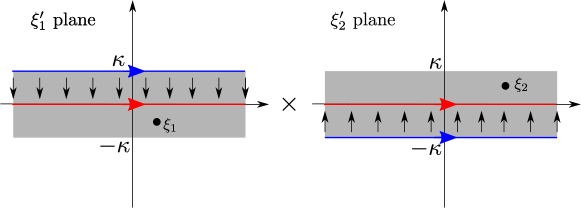
Figure 3.3: Illustration of the contour deformation when passing from (3.10) to (3.12)

This deformation of the integration surface does not change the value of the integral due to the 2D analog of Cauchy’s theorem or Stokes’ theorem [48]. Thus, for ${\rm Im}(\xi_{1})<0$, ${\rm Im}(\xi_{2})>0$ the continuation is given by a slightly modified formula instead of (3.10):

$$\tilde{W}(\xi_{1},\xi_{2}) = \frac{\gamma(\xi_{1},\xi_{2})}{4\pi^{2}}\int\limits_{-\infty}^{\infty}\mathrm{d}\xi_{2}^{\prime}\int\limits_{-\infty}^{\infty}\mathrm{d}\xi_{1}^{\prime}\,\frac{\gamma(\xi_{1},-\xi_{2}^{\prime})\,\tilde{K}(\xi_{1}^{\prime},\xi_{2}^{\prime})\,\tilde{W}(\xi_{1}^{\prime},\xi_{2}^{\prime})}{(\xi_{1}^{\prime}-\xi_{1})(\xi_{2}^{\prime}-\xi_{2})}$$ (3.12)

$$+ \frac{i\gamma(\xi_{1},\xi_{2})\,\gamma(\xi_{1},k_{2})}{(\xi_{1}+k_{1})(\xi_{2}+k_{2})}.$$

Using this formula, we can continue $\tilde{W}$ into the domain $(H^{-}\setminus\{-k_{1}\})\times\hat{H}^{+}$:

Theorem 3.3.

The function $\tilde{W}(\xi_{1},\xi_{2})$ is analytic in the domain ${(H^{-}\setminus\{-k_{1}\})\times\hat{H}^{+}}$. In the vicinity of $\{-k_{1}\}\times\hat{H}^{+}$ the function can be represented as

$$\tilde{W}(\xi_{1},\xi_{2})=\frac{1}{\xi_{1}+k_{1}}\frac{i\,\gamma(k_{1},\xi_{2})\gamma(k_{1},k_{2})}{\xi_{2}+k_{2}}+O((\xi_{1}+k_{1})^{0})$$ (3.13)

The function is analytic on the boundary elements $\mathbb{R}\times\hat{H}^{+}$, $P\times\hat{H}^{+}$, $H^{-}\times\mathbb{R}$, and continuous on the boundary element $P\times\mathbb{R}$.

Remark 3.4.

One can see that we are going to prove analyticity in the domain $B_{1}\times B_{2}$ (of real dimension 4), where $B_{1}=H^{-}$, $B_{2}=\hat{H}^{+}$ (minus the polar set), analyticity at the points of the boundary $(\partial B_{1}\times B_{2})\cup(B_{1}\times\partial B_{2})$ (of real dimension 3) and continuity at the points of the skeleton of the boundary $(\partial B_{1}\times\partial B_{2})$ (of real dimension 2).

Analyticity at any point of $(\partial B_{1}\times B_{2})\cup(B_{1}\times\partial B_{2})$ has the sense that the function can be analytically continued to a small polydisc with the center at such point.

Continuity of the function at the points belonging to $(\partial B_{1}\times\partial B_{2})$ means that the function tends to a certain common limit while the argument tends to the point along any continuous path going in the domain $(B_{1}\times B_{2})\cup(\partial B_{1}\times B_{2})\cup(B_{1}\times\partial B_{2})$.

Proof.

Let us start by analysing the integral in (3.12):

$$J(\xi_{1},\xi_{2})\equiv\int\limits_{-\infty}^{\infty}\mathrm{d}\xi_{2}^{\prime}\int\limits_{-\infty}^{\infty}\mathrm{d}\xi_{1}^{\prime}\,\frac{\gamma(\xi_{1},-\xi_{2}^{\prime})\,\tilde{K}(\xi_{1}^{\prime},\xi_{2}^{\prime})\,\tilde{W}(\xi_{1}^{\prime},\xi_{2}^{\prime})}{(\xi_{1}^{\prime}-\xi_{1})(\xi_{2}^{\prime}-\xi_{2})}.$$

Domain of analyticity of $J$.

First of all, the integral converges due to the growth conditions (2.18)–(2.20) of the functional problem. Let us now study all factors of the integrand and make sure that neither of them is singular for $\xi_{1}\in H^{-}\setminus\{-k_{1}\}$ and $\xi_{2}\in\hat{H}^{+}$.

The functions $\tilde{K}(\xi_{1}^{\prime},\xi_{2}^{\prime})$ and $\tilde{W}(\xi_{1}^{\prime},\xi_{2}^{\prime})$ do not depend on $\xi_{1},\xi_{2}$ and do not pose any problem.

The polar factors $(\xi_{1}^{\prime}-\xi_{1})^{-1}$ and $(\xi_{2}^{\prime}-\xi_{2})^{-1}$ are regular since $\xi_{1,2}$ are not real, while $\xi_{1,2}^{\prime}$ are.

The factor $\gamma(\xi_{1},-\xi_{2}^{\prime})=\sqrt{\sqrt{k^{2}-\xi_{1}^{2}}-\xi_{2}^{\prime}}$ would have branch points for $\xi_{1}=\pm k$ and $\sqrt{k^{2}-\xi_{1}^{2}}=\xi_{2}^{\prime}$. However $\pm k\notin H^{-}$ by definition of $H^{-}$ and, since $\xi_{1}\in H^{-}$, we know by Lemma 3.2 that $\sqrt{k^{2}-\xi_{1}^{2}}$ belongs to $H^{+}$ which does not contain the real number $\xi_{2}^{\prime}$.

Therefore, $J$ is convergent and its integrand is analytic in ${(H^{-}\setminus\{-k_{1}\})\times\hat{H}^{+}}$. Hence, since Morera’s theorem holds in two complex variables (see [48]), $J$ is analytic in this domain.

Analyticity of $J$ on the boundary.

The fact that $J(\xi_{1},\xi_{2})$ is analytic at the points of $\mathbb{R}\times\hat{H}^{+}$, $H^{-}\times\mathbb{R}$ and $P\times\hat{H}^{+}$ is supported by the possibility to use Cauchy’s theorem and change the integration surface to a product $\Theta_{1}\times\Theta_{2}$, where contours $\Theta_{1}$ and $\Theta_{2}$ are contained within the strip $|{\rm Im}(\xi)|<\kappa$.

Let us consider a point $(\xi_{1}^{\star},\xi_{2}^{\star})\in\mathbb{R}\times\hat{H}^{+}$ (Step 1). First of all, the term $\gamma(\xi_{1},-\xi_{2}^{\prime})$ is analytic at $\xi_{1}^{\star}$ since $\xi_{1}^{\star}\notin h^{\pm}$. The term that is actually problematic is the polar factor $(\xi_{1}-\xi_{1}^{\prime})^{-1}$. To avoid this problem, first consider $(\xi_{1},\xi_{2}^{\star})$, with $\xi_{1}\in H^{-}$ (Step 2). From what we saw above, $J$ is clearly analytic there. Moreover its integrand (as a function of $(\xi_{1}^{\prime},\xi_{2}^{\prime})$) is analytic within the strip $|\text{Im}(\xi_{1}^{\prime})|<\kappa$. Hence, as illustrated in Fig. 3.4, we can deform the contour up from $\mathbb{R}$ to $\Theta_{1}=(-\infty+i\kappa^{\prime},\infty+i\kappa^{\prime})$ without changing the value of $J$ (Step 3). Now we can safely let $\xi_{1}$ move towards $\xi_{1}^{\star}$ from within $H^{-}$, without hitting the singularity of the polar factor $(\xi_{1}-\xi_{1}^{\prime})^{-1}$. Hence $J$ can be analytically continued on $\mathbb{R}\times\hat{H}^{+}$.

Figure 3.4: Illustration of the contour deformation needed to prove analyticity on $\mathbb{R}\times\hat{H}^{+}$

Let us now consider a point $(\xi_{1}^{\star},\xi_{2}^{\star})\in H^{-}\times\mathbb{R}$ (Step 1). This time the problematic term is the polar factor $(\xi_{2}-\xi_{2}^{\prime})^{-1}$, which may become singular at $\xi_{2}^{\star}$. Hence, we want to deform the contour down in the $\xi_{2}^{\prime}$ plane, but this time we need to be a little bit more careful. Consider a point $(\xi_{1}^{\star},\xi_{2})$, with $\xi_{2}\in\hat{H}^{+}$ (Step 2). Note that at this stage, the singular loci of the function $\gamma(\xi_{1},-\xi_{2}^{\prime})$ is $h^{-}$. Now, as illustrated in Fig. 3.5, when deforming the contour down to a new contour $\Theta_{2}$, this singular loci becomes a curve surrounding $h^{-}$. Hence when deforming the contour down, one should be careful that this loci does not intersect the point $\xi_{1}^{\star}$ (Step 3). Note that since $\xi_{1}^{\star}\notin h^{-}$, it is always possible to find a $\kappa^{\prime}>0$ small enough such that this isn’t the case. Let us choose $\Theta_{2}=(-\infty-i\kappa^{\prime},\infty-i\kappa^{\prime})$ so that this deformation does not affect the value of $J(\xi_{1}^{\star},\xi_{2})$. We can then safely let $\xi_{2}$ move towards $\xi_{2}^{\star}$ from within $\hat{H}^{+}$, without hitting the singularity of the polar factor $(\xi_{2}-\xi_{2}^{\prime})^{-1}$. Hence $J$ can be analytically continued on $H^{-}\times\mathbb{R}$.

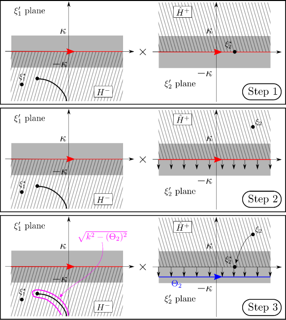
Figure 3.5: Illustration of the contour deformation needed to prove analyticity on $\mathbb{H^{-}}\times\mathbb{R}$

Finally, let us consider a point $(\xi_{1}^{\star},\xi_{2}^{\star})\in P\times\hat{H}^{+}$ (Step 1). Here the polar factors do not present any issues, however, the function $\gamma(\xi_{1},-\xi_{2}^{\prime})$ does. Its singular loci in the $\xi_{1}$ plane for $\xi_{2}^{\prime}\in\mathbb{R}$ is $P$, while its singular loci in the $\xi_{2}^{\prime}$ plane for $\xi_{1}\in P$ is $\mathbb{R}$. Let us further assume that $\xi_{1}^{\star}$ is on the right shore of $P$ as illustrated in Fig. 3.6 (the left shore case is very similar). The problematic point in the $\xi_{2}^{\prime}$ plane is $\sqrt{k^{2}-(\xi_{1}^{\star})^{2}}$ which is a branch point of the function $\gamma(\xi_{1}^{\star},-\xi_{2}^{\prime})$ and also belongs to the contour of integration. As before, we will endeavour to deform the contour to avoid this problem. Let us consider $\xi_{1}\in H^{-}$ (Step 2). Now, deform the contour to a contour $\Theta_{2}$ indented below $\sqrt{k^{2}-(\xi_{1}^{\star})^{2}}$ and above $-\sqrt{k^{2}-(\xi_{1}^{\star})^{2}}$ (Step 3). As illustrated in Fig. 3.6, this has for effect to deflect the singular loci in the $\xi_{1}$ plane away from $\xi_{1}^{\star}$, while ensuring that its two shores do not cross in the process. The value of $J(\xi_{1},\xi_{2}^{\star})$ remain unchanged by such deformation. It is now possible to let $\xi_{1}$ approach $\xi_{1}^{\star}$ freely from within $H^{-}$ without hitting any singularity, and so $J$ can be analytically continued to $(\xi_{1}^{\star},\xi_{2}^{\star})$.

Figure 3.6: Illustration of the contour deformation needed to prove analyticity on $P\times\hat{H}^{+}$

Continuity of $J$ on the skeleton.

We shall now focus on proving the continuity of $J(\xi_{1},\xi_{2})$ at a point $(\xi_{1}^{\star},\xi_{2}^{\star})\in P\times\mathbb{R}$, when this point is approached form within $H^{-}\times\hat{H}^{+}$ possibly including parts of the boundary considered above. In order to do so, decompose $\tilde{W}$ as $\tilde{W}=\tilde{W}_{1}+\tilde{W}_{2}$, where

$$\tilde{W}_{1}(\xi_{1}^{\prime},\xi_{2}^{\prime};\xi_{2})=\tilde{W}(\xi_{1}^{\prime},\xi_{2}^{\prime})-\tilde{W}(\xi_{1}^{\prime},{\rm Re}(\xi_{2})) \tilde{W}_{2}(\xi_{1}^{\prime},\xi_{2}^{\prime};\xi_{2})=\tilde{W}(\xi_{1}^{\prime},{\rm Re}(\xi_{2})).$$ and

This naturally decomposes $J$ into $J_{1}+J_{2}$. The first term is continuous as $\xi_{2}\rightarrow\xi_{2}^{\star}$, since the factor $(\xi_{2}^{\prime}-\xi_{2})$ is now a removable singularity and so $J_{1}$ is continuous. The second term does have a polar singularity, though all the other terms are well behaved, and we can calculate the $\xi_{2}^{\prime}$ integral of $J_{2}$ using a residue that behaves like

$$\frac{\gamma(\xi_{1},-\xi_{2}^{\star})}{\xi_{1}^{\prime}-\xi_{1}}\tilde{K}(\xi_{1}^{\prime},\xi_{2}^{\star})\tilde{W}(\xi_{1}^{\prime},\xi_{2}^{\star}),$$

which is continuous as $\xi_{1}\rightarrow\xi_{1}^{\star}$. Hence, the integral possesses the required continuity.

External factor and additive term.

The factor $\gamma(\xi_{1},\xi_{2})$ in front of the integral is analytic by Lemma 3.2. Indeed, since $\xi_{1}\in H^{-}$, $\sqrt{k^{2}-\xi_{1}^{2}}$ belongs to $H^{+}$ and cannot be equal to $-\xi_{2}$ since $\xi_{2}\in\hat{H}^{+}$. The analyticity and the continuity on the boundary can be established in a straightforward way. The additive term can also be analysed directly, and it fits the theorem. In particular, the only singularity of $\tilde{W}$ in the domain $H^{-}\times\hat{H}^{+}$ is due to this term. ∎

Using the modification of (3.11) written as

$$\tilde{W}(\xi_{1},\xi_{2})=\frac{\gamma(\xi_{2},\xi_{1})}{4\pi^{2}}\int\limits_{-\infty}^{\infty}\mathrm{d}\xi_{1}^{\prime}\int\limits_{-\infty}^{\infty}\mathrm{d}\xi_{2}^{\prime}\,\frac{\gamma(\xi_{2},-\xi_{1}^{\prime})\,\tilde{K}(\xi_{1}^{\prime},\xi_{2}^{\prime})\,\tilde{W}(\xi_{1}^{\prime},\xi_{2}^{\prime})}{(\xi_{1}^{\prime}-\xi_{1})(\xi_{2}^{\prime}-\xi_{2})}$$ (3.14)

$$\qquad\qquad\qquad\qquad\qquad\qquad+\frac{i\gamma(\xi_{2},\xi_{1})\,\gamma(\xi_{2},k_{1})}{(\xi_{1}+k_{1})(\xi_{2}+k_{2})},$$

valid for ${\rm Im}(\xi_{1})>0$, ${\rm Im}(\xi_{2})<0$, one can prove the “symmetrical” theorem:

Theorem 3.5.

The function $\tilde{W}(\xi_{1},\xi_{2})$ is analytic in the domain $\hat{H}^{+}\times(H^{-}\setminus\{-k_{2}\})$. In the vicinity of $\hat{H}^{+}\times\{-k_{2}\}$ the function can be represented as

$$\tilde{W}(\xi_{1},\xi_{2})=\frac{1}{\xi_{2}+k_{2}}\frac{i\,\gamma(k_{2},\xi_{1})\gamma(k_{2},k_{1})}{\xi_{1}+k_{1}}+O((\xi_{2}+k_{2})^{0}).$$ (3.15)

The function is analytic on the boundary elements $\hat{H}^{+}\times\mathbb{R}$, $\hat{H}^{+}\times P$, $\mathbb{R}\times H^{-}$, and continuous on the boundary element $\mathbb{R}\times P$.

3.5 Second step of analytical continuation

The second step of our analytical continuation will be based on a deformation of the integration surface in (3.12) into a product $\mathbb{R}\times P$, resulting in the following theorem:

Theorem 3.6.

The function $\tilde{W}$ obeys the following relation:

$$\tilde{W}(\xi_{1},\xi_{2}) = \frac{\gamma(\xi_{1},\xi_{2})}{4\pi^{2}}\int\limits_{P}\mathrm{d}\xi_{2}^{\prime}\int\limits_{-\infty}^{\infty}\mathrm{d}\xi_{1}^{\prime}\frac{\gamma(\xi_{1},-\xi_{2}^{\prime})\,\tilde{K}(\xi_{1}^{\prime},\xi_{2}^{\prime})\,\tilde{W}(\xi_{1}^{\prime},\xi_{2}^{\prime})}{(\xi_{1}^{\prime}-\xi_{1})(\xi_{2}^{\prime}-\xi_{2})}$$ (3.16)

$$+ \frac{i\gamma(\xi_{1},\xi_{2})\,\gamma(\xi_{1},k_{2})\,\gamma(k_{2},k_{1})}{(\xi_{1}+k_{1})\,(\xi_{2}+k_{2})\,\gamma(k_{2},-\xi_{1})},$$

where the left-hand side is defined in the domain $-\kappa<{\rm Im}(\xi_{1})<0$, $0<{\rm Im}(\xi_{2})<\kappa$.

Remark 3.7.

The unknown function $\tilde{W}(\xi_{1}^{\prime},\xi_{2}^{\prime})$ in the right-hand side is defined by Theorem 3.3. Namely, the values on $\mathbb{R}\times P$ are defined by continuity from the values defined by formula (3.12). This is not used, but for most of the points of $\mathbb{R}\times P$ (for all non-singular points) the values of $\tilde{W}$ can be found from integral of the form (3.12) with appropriate integration surfaces.

The factor $\tilde{K}(\xi_{1}^{\prime},\xi_{2}^{\prime})$ is singular at the points of $\mathbb{R}\times P$ where $\xi_{1}^{\prime 2}+\xi_{2}^{\prime 2}=k^{2}$, however, they produce an integrable singularity. The branch of $\tilde{K}(\xi_{1}^{\prime},\xi_{2}^{\prime})$ is chosen by continuity (the choice is defined by physical reasons on $\mathbb{R}\times\mathbb{R}$, then, by continuity, on $\mathbb{R}\times P$). Thus the integral (3.16) can be considered as an improper integral.

Proof.

Let us modify the continuation formula (3.12) as follows. Swap the order of integration, fix $\xi_{1}^{\prime}\in\mathbb{R}$ and deform the contour of integration in $\xi_{2}^{\prime}$ from the real axis to $P$. Note that the function $\tilde{W}$ is analytic between the new and the old contour (apart from a pole at $\xi_{2}^{\prime}=-k_{2}$, which will be taken into account later) according to Theorem 3.5.

While the contour in $\xi_{2}^{\prime}$ is deformed, it hits no singularities of the factor $\tilde{K}(\xi_{1}^{\prime},\xi_{2}^{\prime})$, since for real $\xi_{1}^{\prime}$ the singularities for $\xi_{2}^{\prime}$ are located only on $P$ and $-P$. The contour also does not hit singularities of $\gamma(\xi_{1},-\xi_{2}^{\prime})$ since, by Lemma 3.2, $\sqrt{k^{2}-\xi_{1}^{2}}$ belongs to $H^{+}$ for $-\kappa<{\rm Im}(\xi_{1})<0$, and $\xi_{2}^{\prime}$ belongs to $H^{-}$. Finally, the contour does not hit the singularity of the polar factor $(\xi_{2}^{\prime}-\xi_{2})^{-1}$ for an obvious reason.

Thus, the contour deformation (taking into account an additional loop around the pole $-k_{2}$) obeys the condition of 1D Cauchy’s theorem, and it does not change the integral.

When such a deformation is made, the contour hits this pole at $\xi_{2}^{\prime}=-k_{2}$ (and no other singularity of the integrand). The residue of the integrand at that point can be obtained by Theorem 3.5, and is

$$\frac{-i\gamma(\xi_{1},k_{2})\tilde{K}(\xi_{1}^{\prime},-k_{2})\gamma(k_{2},\xi_{1}^{\prime})\gamma(k_{2},k_{1})}{(k_{2}+\xi_{2})(\xi_{1}^{\prime}+k_{1})(\xi_{1}^{\prime}-\xi_{1})}.$$

It is then necessary to integrate $-2i\pi$ times this residue over $\xi_{1}^{\prime}$. It turns out that the integral is just a Cauchy sum-split integral of a function that only has a pole at $-k_{1}$ in the $\xi_{1}^{\prime}$ plane. The split can hence be performed explicitly by the pole removal technique. This leads to two terms as follows

$$\frac{i\gamma(\xi_{1},\xi_{2})\,\gamma(\xi_{1},k_{2})\,\gamma(k_{2},k_{1})}{(\xi_{1}+k_{1})\,(\xi_{2}+k_{2})\,\gamma(k_{2},-\xi_{1})}-\frac{i\gamma(\xi_{1},\xi_{2})\,\gamma(\xi_{1},k_{2})}{(\xi_{1}+k_{1})\,(\xi_{2}+k_{2})},$$

where the right part of the equality (3.9) has been used. The second term cancels with the second term of (3.10) and the theorem is proved. ∎

The domain of validity of formula (3.16) given in Theorem 3.6 intersects with the domain of natural analyticity of $\tilde{W}$, i.e. ${\rm Im}(\kappa_{1})>-2\kappa$, ${\rm Im}(\kappa_{2})>-2\kappa$. Thus, formula (3.16) can provide an analytical continuation of $\tilde{W}$. Theorems 3.3 and 3.5 perform a continuation into the domains ${\rm Im}(\xi_{1})\leq 0$, ${\rm Im}(\xi_{2})\geq 0$ and ${\rm Im}(\xi_{1})\geq 0$, ${\rm Im}(\xi_{2})\leq 0$ with some cuts. Here our aim is to continue this function into the domain ${\rm Im}(\xi_{1})\leq 0$, ${\rm Im}(\xi_{2})\leq 0$ (also with some cuts).

We find that it is convenient to study a continuation of $-i\tilde{K}\,\tilde{W}$ instead of $\tilde{W}$. Indeed, these functions are the same up to a factor known explicitly. The required continuation is obtained from the following theorem.

Theorem 3.8.

The function $\tilde{U}$ defined by

$$\tilde{U}(\xi_{1},\xi_{2})\equiv-i\tilde{K}(\xi_{1},\xi_{2})\,\tilde{W}(\xi_{1},\xi_{2})$$

can be analytically continued to the domain $(H^{-}\setminus\{-k_{1}\})\times(H^{-}\setminus\{-k_{2}\})$. The residues of $\tilde{U}$ at $\xi_{1}=-k_{1}$ and $\xi_{2}=-k_{2}$ are given by the following asymptotics:

$$\tilde{U}(\xi_{1},\xi_{2})=\frac{1}{\xi_{1}+k_{1}}\frac{\gamma(k_{1},k_{2})}{\gamma(k_{1},-\xi_{2})\,(\xi_{2}+k_{2})}+O((\xi_{1}+k_{1})^{0})$$ (3.17)

$$\tilde{U}(\xi_{1},\xi_{2})=\frac{1}{\xi_{2}+k_{2}}\frac{\gamma(k_{2},k_{1})}{\gamma(k_{2},-\xi_{1})\,(\xi_{1}+k_{1})}+O((\xi_{2}+k_{2})^{0})$$ (3.18)

The function is continuous at $P\times P$

Remark 3.9.

Similarly to what has been done for Theorem 3.3, one can prove that $\tilde{U}$ is analytic on the parts of the boundary $(H^{-}\setminus\{-k_{1}\})\times P$ and $P\times(H^{-}\setminus\{-k_{2}\})$. However, we do not need this result and skip the corresponding argument. The continuity of $\tilde{U}$ on $P\times P$ is still important. It is understood in the sense that for any path in $(H^{-}\setminus\{-k_{1}\})\times(H^{-}\setminus\{-k_{2}\})$ ending at some point of $P\times P$ there exists a limit depending only on the ending point to which $\tilde{U}$ tends along this path.

Proof.

Use the central part of the equality (3.9) to rewrite the formula (3.16) as follows:

$$\tilde{U}(\xi_{1},\xi_{2}) = \frac{1}{4\pi^{2}i\,\gamma(\xi_{1},-\xi_{2})}\int\limits_{P}\mathrm{d}\xi_{2}^{\prime}\int\limits_{-\infty}^{\infty}\mathrm{d}\xi_{1}^{\prime}\frac{\gamma(\xi_{1},-\xi_{2}^{\prime})\,\tilde{K}(\xi_{1}^{\prime},\xi_{2}^{\prime})\,\tilde{W}(\xi_{1}^{\prime},\xi_{2}^{\prime})}{(\xi_{1}^{\prime}-\xi_{1})(\xi_{2}^{\prime}-\xi_{2})}$$ (3.19)

$$+ \frac{\gamma(\xi_{1},k_{2})\,\gamma(k_{2},k_{1})}{(\xi_{1}+k_{1})\,(\xi_{2}+k_{2})\,\gamma(k_{2},-\xi_{1})\,\gamma(\xi_{1},-\xi_{2})},$$

and consider the integral

$$J(\xi_{1},\xi_{2})\equiv\int\limits_{P}\mathrm{d}\xi_{2}^{\prime}\int\limits_{-\infty}^{\infty}\mathrm{d}\xi_{1}^{\prime}\frac{\gamma(\xi_{1},-\xi_{2}^{\prime})\,\tilde{K}(\xi_{1}^{\prime},\xi_{2}^{\prime})\,\tilde{W}(\xi_{1}^{\prime},\xi_{2}^{\prime})}{(\xi_{1}^{\prime}-\xi_{1})(\xi_{2}^{\prime}-\xi_{2})}.$$

First, continue it from the domain $-\kappa<{\rm Im}(\xi_{1})<0$, $0<{\rm Im}(\xi_{2})<\kappa$ to the domain $-\kappa<{\rm Im}(\xi_{1})<0$, $-\kappa<{\rm Im}(\xi_{2})<\kappa$. This continuation causes no problem since the only factor in the integrand depending on $\xi_{2}$ is $(\xi_{2}^{\prime}-\xi_{2})^{-1}$ and it is regular if $\xi_{2}^{\prime}\in P$.

Then consider $J(\xi_{1},\xi_{2})$ with $\xi_{1}$ and $\xi_{2}$ varying in the domain $H^{-}$. This will provide analytical continuation of $J$ into $H^{-}\times H^{-}$. As in the proof of Theorem 3.3, we need to make sure that the integrand is analytic. Using Lemma 3.2, we conclude that the factor $\gamma(\xi_{1},-\xi_{2}^{\prime})$ is analytic for $\xi_{1}\in H^{-}$, $\xi_{2}\in P$. The polar factors are also regular for $\xi_{1,2}\in H^{-}$, $\xi_{1}^{\prime}\in\mathbb{R}$, $\xi_{2}^{\prime}\in P$, and since $\tilde{K}(\xi_{1}^{\prime},\xi_{2}^{\prime})\tilde{W}(\xi_{1}^{\prime},\xi_{2}^{\prime})$ does not depend on $\xi_{1,2}$, this proves the analyticity of $J$.

The external factor $\gamma^{-1}(\xi_{1},-\xi_{2})$ is also analytic on $H^{-}\times H^{-}$ by Lemma 3.2 ($\sqrt{k_{2}-\xi_{1}^{2}}\in H^{+}$, while $\xi_{2}\in H^{-}$). It should be noted that we changed the unknown from $\tilde{W}$ to $\tilde{U}$ in this theorem (comparatively, say, with Theorem 3.3) to prevent the external factor from having singularities in the domain of continuation.

We now need to consider the explicit additive term. One can see once more due to Lemma 3.2 that $\gamma(\xi_{1},-\xi_{2})$, $\gamma(k_{2},-\xi_{1})$ and $\gamma(\xi_{1},k_{2})$ are analytic. Hence the only singularities of this additive term in $H^{-}\times H^{-}$ are the simple poles $\xi_{1}=-k_{1}$ and $\xi_{2}=-k_{2}$, leading to the correct asymptotic behaviour (3.17) and (3.18).

The continuity on $P\times P$ can be proven as in Theorem 3.3. The problematic term comes from the polar factor $(\xi_{2}^{\prime}-\xi_{2})$ and can be dealt with by decomposing $\tilde{W}$ into two parts, a regular one and one that can be studied explicitly.

∎

4 Additive crossing of branch lines

4.1 Singular 2-lines

Unlike the 1D case, in 2D complex analysis the basic singularities are not isolated points, but (analytic) manifolds of real dimension 2 and of complex dimension 1. Below we call these manifolds 2-lines. Among these singularities, we are interested in simple poles and branch 2-lines.

A primitive way to reveal the type of the singularity of a function $f$ is to introduce the local complex coordinates near some point of the singularity, one tangential and one transversal $(\tau,\nu)$, fix the value of the tangential coordinate $\tau$ and see what happens with $f$ as a function of a single variable $\nu$ at the singularity $\nu=0$. For polar 2-lines it will be a pole, and for branch lines of order $m$ it will be a branch point of order $m$.

According to Theorems 3.3 and 3.8, we can state that $\xi_{1}=-k_{1}$ and $\xi_{2}=-k_{2}$ are polar 2-lines of $\tilde{W}(\xi_{1},\xi_{2})$, and some fragments of the “circle” $\xi_{1}^{2}+\xi_{2}^{2}=k^{2}$ are branch 2-lines of order 2. These singularities are not unexpected. The polar lines are the poles of the right-hand side of the Wiener–Hopf equation, and the branch 2-line is that of the coefficient of the equation. The same behavior is demonstrated by the solution of the 1D Wiener–Hopf equation.

What is new in the 2D case, is the appearance of the branch 2-lines $\xi_{1}=-k$ and $\xi_{2}=-k$. Note that in Theorem 3.8 we could prove the analyticity of $\tilde{U}$ in a product of domains cut along the lines $h^{-}$ going from $-k$. A considerably more sophisticated analysis shows that $\xi_{1}=-k$ and $\xi_{2}=-k$ are branch lines of order 2 (we will actually not use this fact in our consideration). Some important remarks about the link between the singularities of $\tilde{W}$ and the properties of the wave field can be found in Appendix B.

We will now show that there is an important concept related to the lines, $\xi_{1}=-k$ and $\xi_{2}=-k$, namely the concept of additive crossing of branch 2-lines. The next section is dedicated to this concept.

4.2 The concept of additive crossing

Let $\eta_{1}$ and $\eta_{2}$ be some (local) complex variables, and let $\eta_{1}=0$ and $\eta_{2}=0$ be branch 2-lines of a function $f(\eta_{1},\eta_{2})$. Let $\eta_{1}=0$ be a branch 2-line of order $m_{1}$, and $\eta_{2}=0$ be a branch 2-line of order $m_{2}$.

Consider the cuts $\chi_{1}$ and $\chi_{2}$ in the complex planes $\eta_{1}$ and $\eta_{2}$, and define the left and the right shores of the cuts as shown in Fig. 4.1.

Figure 4.1: Local coordinates $\eta_{1,2}$

Let $f$ be (locally) represented in the form

$$f(\eta_{1},\eta_{2})=\phi_{1}(\eta_{1},\eta_{2})+\phi_{2}(\eta_{1},\eta_{2})$$ (4.1)

where $\phi_{1}$ has no branching about $\eta_{2}=0$, and $\phi_{2}$ has no branching about $\eta_{1}=0$. Let us now consider $\eta_{1}\in\chi_{1}$ and $\eta_{2}\in\chi_{2}$ and let $\eta_{1,2}^{\rm l,r}$ be these variables taken on the left/right shore of the corresponding cut. It is possible to write down the values of $f$ on different shores of the cuts as follows:

$$f(\eta_{1}^{\rm l},\eta_{2}^{\rm l})=\phi_{1}(\eta_{1}^{\rm l},\eta_{2})+\phi_{2}(\eta_{1},\eta_{2}^{\rm l}),$$

$$f(\eta_{1}^{\rm l},\eta_{2}^{\rm r})=\phi_{1}(\eta_{1}^{\rm l},\eta_{2})+\phi_{2}(\eta_{1},\eta_{2}^{\rm r}),$$

$$f(\eta_{1}^{\rm r},\eta_{2}^{\rm l})=\phi_{1}(\eta_{1}^{\rm r},\eta_{2})+\phi_{2}(\eta_{1},\eta_{2}^{\rm l}),$$

$$f(\eta_{1}^{\rm r},\eta_{2}^{\rm r})=\phi_{1}(\eta_{1}^{\rm r},\eta_{2})+\phi_{2}(\eta_{1},\eta_{2}^{\rm r}).$$

When there is no upper index “l” or “r”, it means that the function is regular on the cut, and the index does not matter. One can see directly that we have

$$f(\eta_{1}^{\rm l},\eta_{2}^{\rm l})+f(\eta_{1}^{\rm r},\eta_{2}^{\rm r})=f(\eta_{1}^{\rm l},\eta_{2}^{\rm r})+f(\eta_{1}^{\rm r},\eta_{2}^{\rm l}).$$ (4.2)

This property is the origin of the following definition.

Definition 4.1.

We say that a function $f(\eta_{1},\eta_{2})$ with branch 2-lines at $\eta_{1}=0$ and $\eta_{2}=0$ has the additive crossing property if the equation (4.2) holds for some appropriate cuts.

We have hence seen that if $f$ can be locally represented by (4.1), then it has the additive crossing property.

Conversely, assume now that a function $f$ has the additive crossing property, i.e. that (4.2) is valid. If we also assume that $f$ can be represented as a Puiseux series in some vicinity of the origin as follows:

$$f(\eta_{1},\eta_{2})=\sum_{n_{1},n_{2}\in\mathbb{Z}}a_{n_{1},n_{2}}\eta_{1}^{n_{1}/m_{1}}\eta_{2}^{n_{2}/m_{2}},$$ (4.3)

then, writing $\eta_{1,2}^{\rm l}=r_{1,2}e^{i\theta_{1,2}}$ and $\eta_{1,2}^{\rm r}=r_{1,2}e^{i(\theta_{1,2}+2\pi)}$, for each term of (4.3), the additive crossing property (4.2) leads to

$$1+e^{2\pi in_{1}/m_{1}}e^{2\pi in_{2}/m_{2}}=e^{2\pi in_{1}/m_{1}}+e^{2\pi in_{2}/m_{2}}.$$ (4.4)

This implies that

$$(1-e^{2\pi in_{1}/m_{1}})(1-e^{2\pi in_{2}/m_{2}})=0,$$

and hence, each allowed term should have no branching either about $\eta_{1}=0$ or about $\eta_{2}=0$. Therefore $f$ can be locally represented by (4.1), with each term of the series belonging either to $\phi_{2}$ or to $\phi_{1}$.

Remark 4.2.

Note that, strictly speaking, it is not necessary for $\eta_{1}=0$ and $\eta_{2}=0$ to be branch 2-lines of the function $f$ in order to define the concept of additive crossing. It is indeed sufficient to require $f(\eta_{1},\eta_{2})$ to be analytic in a domain $(D\setminus\chi_{1})\times(D\setminus\chi_{2})$, where $D$ is some neighbourhood of the origin of a 1D complex plane, such that $f$ is continuous on the sides of the cuts (to make $f(\eta_{1}^{\rm l,r},\eta_{2}^{\rm l,r})$ well defined). Then the same relation (4.2) will be called the additive crossing property of $f$. In our case we are going to establish the additive crossing property for

$$\eta_{1,2}=\xi_{1,2}+k, f(\eta_{1},\eta_{2})=\tilde{U}^{\prime}(\eta_{1}-k,\eta_{2}-k), \chi_{1,2}=h^{-}+k.$$

4.3 Deformation of the surface of integration for $u(x_{1},x_{2},0)$

Consider the function $\tilde{U}^{\prime}$ defined by (2.17) and introduce its inverse Fourier transform $v(x_{1},x_{2})$ as per (2.8):

$$v(x_{1},x_{2})\equiv\frac{1}{4\pi^{2}}\int\limits_{-\infty}^{\infty}\int\limits_{-\infty}^{\infty}\tilde{U}^{\prime}(\xi_{1},\xi_{2})e^{-i(\xi_{1}x_{1}+\xi_{2}x_{2})}\mathrm{d}\xi_{1}\mathrm{d}\xi_{2}$$ (4.5)

and note that

$$v(x_{1},x_{2})=u(x_{1},x_{2},0)\quad\mbox{ for }\quad(x_{1},x_{2})\in(Q_{2}\cup Q_{3}\cup Q_{4}),$$

and

$$v(x_{1},x_{2})=u(x_{1},x_{2},0^{+})-u^{\rm in}(x_{1},x_{2},0)\quad\mbox{ for }\quad(x_{1},x_{2})\in Q_{1}.$$

Therefore, according to the boundary condition (2.2), it should be equal to zero if $x_{1}>0$ and $x_{2}>0$. Let us consider $x_{1}>0$ and $x_{2}>0$ up to the end of this section.

The exponential factor of the Fourier transform, $e^{-i(\xi_{1}x_{1}+\xi_{2}x_{2})}$, decays in the domain ${\rm Im}(\xi_{1})<0$, ${\rm Im}(\xi_{2})<0$. The function $\tilde{U}^{\prime}(\xi_{1},\xi_{2})$ has two polar 2-lines $\xi_{1}=-k_{1}$ and $\xi_{2}=-k_{2}$. Let us introduce two small loops $\sigma_{1}$ and $\sigma_{2}$ encircling the points $-k_{1}$ and $-k_{2}$ in the anti-clockwise direction.

In the integral (4.5), deform first the $\xi_{1}$ real axis into the contour $P$, and then the $\xi_{2}$ real axis into $P$. At each step, the usual 1D Cauchy’s theorem is used to ensure that the integral preserves its value. The poles are taken care of by using the loops $\sigma_{1,2}$, resulting in:

$$v(x_{1},x_{2})=\frac{1}{4\pi^{2}}\int_{P}\int_{P}\tilde{U}^{\prime}(\xi_{1},\xi_{2})e^{-i(\xi_{1}x_{1}+\xi_{2}x_{2})}\mathrm{d}\xi_{1}\,\mathrm{d}\xi_{2}+S_{1}+S_{2}+S_{12},$$ (4.6)

where

$$S_{1}=-\frac{1}{4\pi^{2}}\int_{P}\int_{\sigma_{1}}\tilde{U}^{\prime}(\xi_{1},\xi_{2})e^{-i(\xi_{1}x_{1}+\xi_{2}x_{2})}\mathrm{d}\xi_{1}\,\mathrm{d}\xi_{2}\,,$$ (4.7)

$$S_{2}=-\frac{1}{4\pi^{2}}\int_{\sigma_{2}}\int_{P}\tilde{U}^{\prime}(\xi_{1},\xi_{2})e^{-i(\xi_{1}x_{1}+\xi_{2}x_{2})}\mathrm{d}\xi_{1}\,\mathrm{d}\xi_{2}\,,$$ (4.8)

$$S_{12}=\frac{1}{4\pi^{2}}\int_{\sigma_{2}}\int_{\sigma_{1}}\tilde{U}^{\prime}(\xi_{1},\xi_{2})e^{-i(\xi_{1}x_{1}+\xi_{2}x_{2})}\mathrm{d}\xi_{1}\,\mathrm{d}\xi_{2}\,.$$ (4.9)

Consider the term $S_{1}$ and use (3.17) and (2.17) to compute the integral about the pole for each $\xi_{2}\in P$ to get

$$S_{1}=\frac{1}{2\pi i}\int_{P}\left(\frac{\gamma(k_{1},k_{2})}{\gamma(k_{1},-\xi_{2})}-1\right)\frac{e^{ik_{1}x_{1}-i\xi_{2}x_{2}}}{\xi_{2}+k_{2}}\mathrm{d}\xi_{2}.$$ (4.10)

Since the integrand has no branching at $\xi_{2}=-k$ nor anywhere on $h^{-}$ (by Lemma 3.2), the integral is equal to zero and hence $S_{1}=0$. Similarly, we can show that $S_{2}=0$.

Finally, compute the double residue $S_{12}$. One can see that the double residue of $\tilde{U}$ coming from (3.17) is compensated with the double residue of the second term of (2.17), and hence we have $S_{12}=0$. Thus,

$$v(x_{1},x_{2})=\frac{1}{4\pi^{2}}\int_{P}\int_{P}\tilde{U}^{\prime}(\xi_{1},\xi_{2})e^{-i(\xi_{1}x_{1}+\xi_{2}x_{2})}\mathrm{d}\xi_{1}\,\mathrm{d}\xi_{2}.$$ (4.11)

The integral (4.11) can be interpreted in terms of the additive crossing property of the 2-lines $\xi_{1}=-k$ and $\xi_{2}=-k$. Consider $h^{-}$ as a (directed) contour going from $-k$ to $-i\infty$. The contour $P$ consists of two parts: one goes along the right shore of $h^{-}$ in the negative direction, and another goes along the left shore in the positive direction (see Fig. 3.2 (right) and Fig. 4.1 ). Thus, one can rewrite (4.11) as follows:

$$v(x_{1},x_{2}) = \frac{1}{4\pi^{2}}\int_{h^{-}}\int_{h^{-}}(\tilde{U}^{\prime}(\xi_{1}^{\rm l},\xi_{2}^{\rm l})+\tilde{U}^{\prime}(\xi_{1}^{\rm r},\xi_{2}^{\rm r})-\tilde{U}^{\prime}(\xi_{1}^{\rm l},\xi_{2}^{\rm r})-\tilde{U}^{\prime}(\xi_{1}^{\rm r},\xi_{2}^{\rm l}))\times$$ (4.12)

$$e^{-i(\xi_{1}x_{1}+\xi_{2}x_{2})}\mathrm{d}\xi_{1}\,\mathrm{d}\xi_{2}.$$

One can see that $v(\xi_{1},\xi_{2})$ is equal to 0 if

$$\tilde{U}^{\prime}(\xi_{1}^{\rm l},\xi_{2}^{\rm l})+\tilde{U}^{\prime}(\xi_{1}^{\rm r},\xi_{2}^{\rm r})-\tilde{U}^{\prime}(\xi_{1}^{\rm l},\xi_{2}^{\rm r})-\tilde{U}^{\prime}(\xi_{1}^{\rm r},\xi_{2}^{\rm l})=0,$$ (4.13)

i.e. if the 2-lines $\xi_{1}=-k$ and $\xi_{2}=-k$ of the function $\tilde{U}^{\prime}$ have the additive crossing property. Hence additive crossing implies 3/4-basedness.

Conversely, a 2D uniqueness theorem (see Appendix C) can be applied to the integral (4.12) to get that if $v(x_{1},x_{2})=0$ in $Q_{1}$ then (4.13) is fulfilled. Thus, we have obtained an equivalence between the 3/4-basedness of $\tilde{U}^{\prime}$ and the additive crossing property of the 2-lines $\xi_{1}=-k$ and $\xi_{2}=-k$. This will allow us to reformulate the functional problem of Section 2.4.

4.4 Reformulation of the functional problem

The main result of the present paper is a reformulation of the functional problem from Section 2.4. Consider the formulation of Theorem 2.4. According to the content of this paper, the first two items of the theorem can be replaced by the following four conditions. The theorem remains valid after the replacement.

• $\tilde{W}(\xi_{1},\xi_{2})$ is analytic in the domain

  $$(\hat{H}^{+}\times(\hat{H}^{+}\cup H^{-}\setminus\{-k_{2}\}))\cup((\hat{H}^{+}\cup H^{-}\setminus\{-k_{1}\})\times\hat{H}^{+}).$$

• $\tilde{W}(\xi_{1},\xi_{2})$ has poles at $\xi_{1}=-k_{1}$, $\xi_{2}=-k_{2}$, the residues of which are defined by (3.13) and (3.15).

• $\tilde{U}^{\prime}(\xi_{1},\xi_{2})$, as defined by (2.17), is analytic in the domain

  $$(H^{-}\setminus\{-k_{1}\})\times(H^{-}\setminus\{-k_{2}\})$$

• $\tilde{U}^{\prime}(\xi_{1},\xi_{2})$ has the additive crossing property for the 2-lines $\xi_{1}=-k$ and $\xi_{2}=-k$ with the cuts $h^{-}$.

Note that the residues (3.17) and (3.18) of $\tilde{U}^{\prime}$ at $\xi_{1}=-k_{1}$ and $\xi_{2}=-k_{2}$ can be obtained by continuation of the residues of $\tilde{W}$. Hence, strictly speaking, it is not necessary to include them in the formulation of the functional problem.

5 Concluding remarks

An important step of the usual 1D Wiener–Hopf method is to draw conclusions about the analyticity properties of unknown functions originally defined by half-range Fourier transforms. This is exactly what we have done here in a 2D context, and this is why we believe that this final reformulation is important. Indeed we drew some conclusions about the domain of analyticity of unknown functions originally defined by 1/4 and 3/4 range Fourier transforms.

We established analyticity of the unknown functions $\tilde{W}$ and $\tilde{U}^{\prime}$ in domains totally forming the $\mathbb{C}\times\mathbb{C}$ space (which agrees with the Wiener–Hopf concept), however, unfortunately, this space contains the branch 2-lines $\xi_{1}=-k$, $\xi_{2}=-k$. Almost nothing is known about this branching and hence, formally, at this level of understanding, the Liouville theorem (which is valid in $\mathbb{C}^{2}$, see e.g. [48]) cannot be applied, and thus the Wiener–Hopf method cannot be completed. We plan to demonstrate in a subsequent paper that the additive crossing property of the branch 2-lines is in fact a very strong condition, and that some important physical features (such as the vertex asymptotics for example) can be recovered from it.

Appendix A Proof of Theorem 3.1

In this appendix, for simplicity, we will use the notations of [47]. That is, we will say that a function of the two variables $(\xi_{1},\xi_{2})$ is a $\circ+$ (resp. $\circ-$) function if it is analytic in the UHP (resp. LHP) of the $\xi_{2}$ plane, when considered a function of $\xi_{2}$ only. Similarly, we say that such a function is a $+\circ$ (resp. $-\circ$) function if it is analytic in the UHP (resp. LHP) of the $\xi_{1}$ plane, when considered a function of $\xi_{1}$ only. We can then naturally define a $+-$ function as a function that is at the same time a $+\circ$ and a $\circ-$ function. Similarly, it is possible to define $++$, $-+$ and $--$ functions. These properties will be indicated as a subscript when necessary.

Rewrite the factorisation as follows:

$$\widetilde{K}(\boldsymbol{\xi})=\widetilde{K}_{\circ+}(\boldsymbol{\xi})\times\widetilde{K}_{\circ-}(\boldsymbol{\xi}), \widetilde{K}_{\circ+}(\boldsymbol{\xi})=\frac{1}{\gamma(\xi_{1},\xi_{2})}, \widetilde{K}_{\circ-}(\boldsymbol{\xi})=\frac{1}{\gamma(\xi_{1},-\xi_{2})}.$$

Starting from the functional equation, we get

$$\tilde{K}(\boldsymbol{\xi})\tilde{W}(\boldsymbol{\xi})=i\tilde{U}(\boldsymbol{\xi})=i\left(\frac{1}{(\xi_{1}+k_{1})(\xi_{2}+k_{2})}+\tilde{U}^{\prime}(\boldsymbol{\xi})\right)$$ (A.1)

Now, since $\tilde{U}^{\prime}$ is 3/4-based, there exists a function $\mathfrak{u}^{\prime}$ such that $\tilde{U}^{\prime}=\mathfrak{F}_{3/4}[\mathfrak{u}^{\prime}]$. We can hence introduce the useful functions $\tilde{U}^{\prime}_{+-}$ and $\tilde{U}^{\prime}_{-\circ}$ by

$$\tilde{U}^{\prime}(\boldsymbol{\xi}) = \mathfrak{F}_{3/4}[\mathfrak{u}^{\prime}](\boldsymbol{\xi})=\iint_{Q_{2}\cup Q_{3}\cup Q_{4}}\mathfrak{u}^{\prime}(\boldsymbol{x})e^{i\boldsymbol{x}\cdot\boldsymbol{\xi}}\,\mathrm{d}\boldsymbol{\xi}$$

$$= \iint_{Q_{4}}\mathfrak{u}^{\prime}(\boldsymbol{x})e^{i\boldsymbol{x}\cdot\boldsymbol{\xi}}\,\mathrm{d}\boldsymbol{\xi}+\iint_{Q_{2}\cup Q_{3}}\mathfrak{u}^{\prime}(\boldsymbol{x})e^{i\boldsymbol{x}\cdot\boldsymbol{\xi}}\,\mathrm{d}\boldsymbol{\xi}=\tilde{U}^{\prime}_{+-}(\boldsymbol{\xi})+\tilde{U}^{\prime}_{-\circ}(\boldsymbol{\xi})$$

Now, using the factorisation of $\tilde{K}$, we get

$$\frac{\tilde{K}_{\circ+}(\boldsymbol{\xi})\tilde{W}(\boldsymbol{\xi})}{i} = \frac{1}{\widetilde{K}_{\circ-}(\boldsymbol{\xi})(\xi_{1}+k_{1})(\xi_{2}+k_{2})}+\frac{\tilde{U}^{\prime}_{+-}(\boldsymbol{\xi})}{\widetilde{K}_{\circ-}(\boldsymbol{\xi})}+\frac{\tilde{U}^{\prime}_{-\circ}(\boldsymbol{\xi})}{\widetilde{K}_{\circ-}(\boldsymbol{\xi})}$$ (A.2)

We will also use various sum-split Cauchy operators, namely $[.]_{\circ+}$, $[.]_{\circ-}$, $[.]_{+\circ}$ and $[.]_{-\circ}$ defined as follows for any function $\tilde{\Phi}(\xi_{1},\xi_{2})$ analytic within a product of strips we have

$${}[\tilde{\Phi}]_{\circ-}(\xi_{1},\xi_{2})=\frac{-1}{2i\pi}\int_{-\infty+i\kappa}^{\infty+i\kappa}\frac{\tilde{\Phi}(\xi_{1},\xi_{2}^{\prime})}{\xi_{2}^{\prime}-\xi_{2}}\,\mathrm{d}\xi_{2}^{\prime} [\tilde{\Phi}]_{\circ+}(\xi_{1},\xi_{2})=\frac{1}{2i\pi}\int_{-\infty-i\kappa}^{\infty-i\kappa}\frac{\tilde{\Phi}(\xi_{1},\xi_{2}^{\prime})}{\xi_{2}^{\prime}-\xi_{2}}\,\mathrm{d}\xi_{2}^{\prime}$$ and

$${}[\tilde{\Phi}]_{-\circ}(\xi_{1},\xi_{2})=\frac{-1}{2i\pi}\int_{-\infty+i\kappa}^{\infty+i\kappa}\frac{\tilde{\Phi}(\xi_{1}^{\prime},\xi_{2})}{\xi_{1}^{\prime}-\xi_{1}}\,\mathrm{d}\xi_{1}^{\prime} [\tilde{\Phi}]_{+\circ}(\xi_{1},\xi_{2})=\frac{1}{2i\pi}\int_{-\infty-i\kappa}^{\infty-i\kappa}\frac{\tilde{\Phi}(\xi_{1}^{\prime},\xi_{2})}{\xi_{1}^{\prime}-\xi_{1}}\,\mathrm{d}\xi_{1}^{\prime}.$$ and

We can hence rewrite (A.2) as

$$\frac{\tilde{K}_{\circ+}(\boldsymbol{\xi})\tilde{W}(\boldsymbol{\xi})}{i} = \frac{1}{\widetilde{K}_{\circ-}(\boldsymbol{\xi})(\xi_{1}+k_{1})(\xi_{2}+k_{2})}+\frac{\tilde{U}^{\prime}_{+-}(\boldsymbol{\xi})}{\widetilde{K}_{\circ-}(\boldsymbol{\xi})}+\left[\frac{\tilde{U}^{\prime}_{-\circ}(\boldsymbol{\xi})}{\widetilde{K}_{\circ-}(\boldsymbol{\xi})}\right]_{\circ-}+\left[\frac{\tilde{U}^{\prime}_{-\circ}(\boldsymbol{\xi})}{\widetilde{K}_{\circ-}(\boldsymbol{\xi})}\right]_{\circ+},$$

and, upon rearranging, we get

$$\frac{\tilde{K}_{\circ+}(\boldsymbol{\xi})\tilde{W}(\boldsymbol{\xi})}{i}-\left[\frac{\tilde{U}^{\prime}_{-\circ}(\boldsymbol{\xi})}{\widetilde{K}_{\circ-}(\boldsymbol{\xi})}\right]_{\circ+} = \frac{\tilde{U}^{\prime}_{+-}(\boldsymbol{\xi})}{\widetilde{K}_{\circ-}(\boldsymbol{\xi})}+\left[\frac{\tilde{U}^{\prime}_{-\circ}(\boldsymbol{\xi})}{\widetilde{K}_{\circ-}(\boldsymbol{\xi})}\right]_{\circ-}+\frac{1}{\widetilde{K}_{\circ-}(\boldsymbol{\xi})(\xi_{1}+k_{1})(\xi_{2}+k_{2})}.$$

The sum-split in the $\xi_{2}$ plane of the term involving the poles can be done explicitly by the pole removal technique to get

$$\frac{1}{\widetilde{K}_{\circ-}(\boldsymbol{\xi})(\xi_{1}+k_{1})(\xi_{2}+k_{2})} = \frac{1}{(\xi_{1}+k_{1})(\xi_{2}+k_{2})}\left(\frac{1}{\widetilde{K}_{\circ-}(\boldsymbol{\xi})}-\frac{1}{\widetilde{K}_{\circ-}(\xi_{1},-k_{2})}\right)$$

$$+ \frac{1}{\widetilde{K}_{\circ-}(\xi_{1},-k_{2})(\xi_{1}+k_{1})(\xi_{2}+k_{2})},$$

which finally leads (LABEL:eq:proofth3part2) to become

$$\frac{\tilde{K}_{\circ+}(\boldsymbol{\xi})\tilde{W}(\boldsymbol{\xi})}{i}-\left[\frac{\tilde{U}^{\prime}_{-\circ}(\boldsymbol{\xi})}{\widetilde{K}_{\circ-}(\boldsymbol{\xi})}\right]_{\circ+}-\frac{1}{\widetilde{K}_{\circ-}(\xi_{1},-k_{2})(\xi_{1}+k_{1})(\xi_{2}+k_{2})} =$$

$$\frac{\tilde{U}^{\prime}_{+-}(\boldsymbol{\xi})}{\widetilde{K}_{\circ-}(\boldsymbol{\xi})}+\left[\frac{\tilde{U}^{\prime}_{-\circ}(\boldsymbol{\xi})}{\widetilde{K}_{\circ-}(\boldsymbol{\xi})}\right]_{\circ-}+\frac{1}{(\xi_{1}+k_{1})(\xi_{2}+k_{2})}\left(\frac{1}{\widetilde{K}_{\circ-}(\boldsymbol{\xi})}-\frac{1}{\widetilde{K}_{\circ-}(\xi_{1},-k_{2})}\right).$$ (A.4)

One can see that the LHS of (A.4) is analytic in the UHP of the $\xi_{2}$ plane, while its RHS is analytic in the LHP of the $\xi_{2}$ plane. Application of Liouville’s theorem in the $\xi_{2}$ plane implies that both sides are zero, leading to

$$\tilde{W}(\boldsymbol{\xi}) = \frac{i}{\widetilde{K}_{\circ-}(\xi_{1},-k_{2})\tilde{K}_{\circ+}(\boldsymbol{\xi})(\xi_{1}+k_{1})(\xi_{2}+k_{2})}+\frac{i}{\tilde{K}_{\circ+}(\boldsymbol{\xi})}\left[\frac{\tilde{U}^{\prime}_{-\circ}(\boldsymbol{\xi})}{\widetilde{K}_{\circ-}(\boldsymbol{\xi})}\right]_{\circ+}$$

$$= \frac{i\gamma(\xi_{1},\xi_{2})\gamma(\xi_{1},k_{2})}{(\xi_{1}+k_{1})(\xi_{2}+k_{2})}+\frac{\gamma(\xi_{1},\xi_{2})}{2\pi}\int_{-\infty-i\kappa}^{\infty-i\kappa}\frac{\tilde{U}^{\prime}_{-\circ}(\xi_{1},\xi_{2}^{\prime})}{(\xi_{2}^{\prime}-\xi_{2})\widetilde{K}_{\circ-}(\xi_{1},\xi_{2}^{\prime})}\,\mathrm{d}\xi_{2}^{\prime}$$

$$= \frac{i\gamma(\xi_{1},\xi_{2})\gamma(\xi_{1},k_{2})}{(\xi_{1}+k_{1})(\xi_{2}+k_{2})}+\frac{\gamma(\xi_{1},\xi_{2})}{2\pi}\int_{-\infty-i\kappa}^{\infty-i\kappa}\frac{\gamma(\xi_{1},-\xi_{2}^{\prime})\tilde{U}^{\prime}_{-\circ}(\xi_{1},\xi_{2}^{\prime})}{(\xi_{2}^{\prime}-\xi_{2})}\,\mathrm{d}\xi_{2}^{\prime}.$$

Let us now note from (A.1) that we have

$$\tilde{U}^{\prime}_{-\circ}(\xi_{1},\xi_{2}^{\prime}) = \left[\frac{\tilde{K}(\xi_{1},\xi_{2}^{\prime})\tilde{W}(\xi_{1},\xi_{2}^{\prime})}{i}\right]_{-\circ}$$ (A.6)

$$= \frac{1}{2\pi}\int_{-\infty+i\kappa}^{\infty+i\kappa}\frac{\tilde{K}(\xi_{1}^{\prime},\xi_{2}^{\prime})\tilde{W}(\xi_{1}^{\prime},\xi_{2}^{\prime})}{\xi_{1}^{\prime}-\xi_{1}}\,\mathrm{d}\xi_{1}^{\prime}.$$

Combining (LABEL:eq:thproofpart5) and (A.6), we obtain

$$\tilde{W}(\boldsymbol{\xi}) = \frac{i\gamma(\xi_{1},\xi_{2})\gamma(\xi_{1},k_{2})}{(\xi_{1}+k_{1})(\xi_{2}+k_{2})}$$

$$+ \frac{\gamma(\xi_{1},\xi_{2})}{2\pi}\int_{-\infty-i\kappa}^{\infty-i\kappa}\frac{\gamma(\xi_{1},-\xi_{2}^{\prime})}{(\xi_{2}^{\prime}-\xi_{2})}\left(\frac{1}{2\pi}\int_{-\infty+i\kappa}^{\infty+i\kappa}\frac{\tilde{K}(\xi_{1}^{\prime},\xi_{2}^{\prime})\tilde{W}(\xi_{1}^{\prime},\xi_{2}^{\prime})}{\xi_{1}^{\prime}-\xi_{1}}\,\mathrm{d}\xi_{1}^{\prime}\right)\,\mathrm{d}\xi_{2}^{\prime}$$

$$= \frac{i\gamma(\xi_{1},\xi_{2})\gamma(\xi_{1},k_{2})}{(\xi_{1}+k_{1})(\xi_{2}+k_{2})}$$

$$+ \frac{\gamma(\xi_{1},\xi_{2})}{4\pi^{2}}\int_{-\infty-i\kappa}^{\infty-i\kappa}\frac{\gamma(\xi_{1},-\xi_{2}^{\prime})}{(\xi_{2}^{\prime}-\xi_{2})}\left(\int_{-\infty+i\kappa}^{\infty+i\kappa}\frac{\tilde{K}(\xi_{1}^{\prime},\xi_{2}^{\prime})\tilde{W}(\xi_{1}^{\prime},\xi_{2}^{\prime})}{\xi_{1}^{\prime}-\xi_{1}}\,\mathrm{d}\xi_{1}^{\prime}\right)\,\mathrm{d}\xi_{2}^{\prime},$$

as required. The proof of the second formula can be obtained in a very similar way by first splitting $\tilde{U}^{\prime}$ as an integral over $Q_{2}$ and an integral over $Q_{3}\cup Q_{4}$, and then perform a sum split of the functional equation in the $\xi_{1}$ plane instead.

Appendix B Singularities of the analytical continuation

Consider the real plane $(\xi_{1},\xi_{2})$ and the function $\tilde{W}(\xi_{1},\xi_{2})$ on this plane. This plane will be called the physical real plane of $(\xi_{1},\xi_{2})$. In the analytical continuation procedure we found the following singularities of $\tilde{W}$:

• a part of the circle $\xi_{1}^{2}+\xi_{2}^{2}=k^{2}$, which is the branch 2-line of the coefficient of the functional equation;

• the branch 2-lines $\xi_{1}=-k$ and $\xi_{2}=-k$ (the cuts $h^{-}$ start at $-k$);

• the polar 2-lines $\xi_{1}=-k_{1}$ and $\xi_{2}=-k_{2}$.

Note that only the part of the circle shown in bold in Fig. B.2 (left) is a singular set on the physical plane. All the rest of the circle belongs to the set of analyticity. This can be shown as follows. Let $\epsilon$ be small positive, and then take the limit $\epsilon\to 0$. Consider a vicinity of the point $\xi_{1}=\cos(\varphi)$, $\xi_{2}=\sin(\varphi)$, namely, consider the complex numbers

$$\xi_{1}=\cos(\varphi)+\mu_{1},\qquad\xi_{2}=\sin(\varphi)+\mu_{2},$$

where $\varphi$ is real, and $\mu_{1,2}$ are small and chosen such that

$$\xi_{1}^{2}+\xi_{2}^{2}=k^{2}=1+i\epsilon.$$

In the linear approximation, this gives

$$\cos(\varphi){\rm Im}(\mu_{1})+\sin(\varphi){\rm Im}(\mu_{2})=\epsilon/2.$$ (B.1)

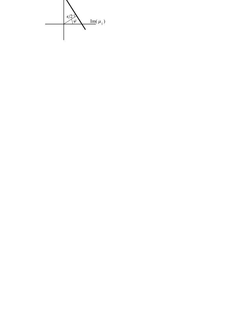
Figure B.1: Straight line structure resulting from (B.1)

The set of values $\text{Im}(\mu_{1,2})$ obeying (B.1) is a line (see Fig. B.1), the slope of which is determined by $\varphi$. One can see that if $-\pi/2<\varphi<\pi$ then this line passes through the zone with ${\rm Im}(\xi_{1})={\rm Im}(\mu_{1})>0$, ${\rm Im}(\xi_{2})={\rm Im}(\mu_{2})>0$. Thus, some singular points appear in the zone of prescribed analyticity of $\tilde{W}$, which is prohibited. Hence, only the part of the circle with $-\pi<\varphi<-\pi/2$ may belong to the common part of the singular set of $\tilde{W}$ and the physical real plane. This part of the circle is shown in Fig. B.2 (left).

Figure B.2: Singularities of $\tilde{W}$ (left) and $\tilde{U}^{\prime}$ (right)

The branching of $\tilde{W}$ on the part of the circle with $-\pi<\varphi<-\pi/2$ can be used to find the asymptotics of the function

$$\frac{\partial u}{\partial n}(-R\cos(\varphi),-R\sin(\varphi),0^{+})\quad\mbox{ as }\quad R\to\infty.$$

For this, the inverse Fourier transform and the saddle point method can be used in a standard way. Note that this function is equal to zero for $-\pi/2<\varphi<\pi$, so the absence of branching at this part of the circle is quite natural.

As we have mentioned, the circle $\xi_{1}^{2}+\xi_{2}^{2}=k^{2}$ corresponds to the singular set of the coefficient of the functional equation, so it can be expected that this set will be a singular set of the solution. This situation reminds the classical 1D Wiener–Hopf method. However, the presence of the branch 2-lines $\xi_{1}=-k$, $\xi_{2}=-k$ is something new that appears only in the 2D case. Physically, however, these branch lines are understandable. They correspond to the edge singularities of the field $u$ having the phase dependencies $\sim e^{ikx_{2}}$ for the edge $x_{1}=0$, and $\sim e^{ikx_{1}}$ for $x_{2}=0$. Thus, in some sense, this corresponds to the edge singularities of the field scattered by the vertex.

Finally, the polar 2-lines $\xi_{1}=-k_{1}$, $\xi_{2}=-k_{2}$ correspond to the cones of rays scattered by the edges. The crossing point $(-k_{1},-k_{2})$ is very important and corresponds to the incident and the reflected plane waves.

Let us now consider the singularities of the function $\tilde{U}^{\prime}$ defined by (2.17). This function is 3/4-based, so its inverse Fourier transform (2.8) should be equal to zero on the quadrant $Q_{1}$. Note that when such a transform is made in $(x_{1},x_{2})\in Q_{1}$, the “contour of integration” should be deformed into the domain ${\rm Im}(\xi_{1})<0$, ${\rm Im}(\xi_{2})<0$, i.e. the continuation established by Theorem 3.8 plays a crucial role.

Three important notes should be made about the singularities of $\tilde{U}^{\prime}$.

1. The polar sets $\xi_{1}=-k_{1}$ and $\xi_{2}=-k_{2}$ are intersecting within the domain $H^{-}\times H^{-}$. This can potentially produce an exponential term, but it is easy to check that the double residue of (3.17), (3.18) is compensated by the explicit term of (2.17) since $\gamma(k_{2},k_{1})/\gamma(k_{2},-k_{1})=1$.

2. Function $\tilde{U}^{\prime}$ is regular at the points of the circle $\xi_{1}^{2}+\xi_{2}^{2}=k^{2}$ corresponding to $-\pi<\varphi<-\pi/2$. The physical reasoning is as follows. Any branching at this point of the circle would lead to a field $u$ with asymptotics $\sim\exp\{ik\sqrt{x_{1}^{2}+x_{2}^{2}}\}$ on $Q_{1}$, which is prohibited by the boundary condition (2.2). The mathematical reasoning is based on Theorem 3.8. If $\epsilon\neq 0$ then the points belonging to this part of the circle belong to the domain $(H^{-}\setminus\{-k_{1}\})\times(H^{-}\setminus\{-k_{2}\})$. Namely, they are points

   $$(-k\cos(\varphi),-k\sin(\varphi))$$

   for some (narrow) complex strip surrounding the real segment $-\pi<\varphi<-\pi/2$. According to Theorem 3.8, at these points $\tilde{U}^{\prime}$ should be regular. Thus, $\tilde{U}^{\prime}$ is allowed to be singular only at the points shown in Fig. B.2 (right).

3. The crossing of branch lines $\xi_{1}=-k$, $\xi_{2}=-k$ belongs to the domain ${\rm Im}(\xi_{1})<0$, ${\rm Im}(\xi_{2})<0$. Potentially, such a crossing can lead to a wave component with the asymptotics $\sim\exp\{ik(x_{1}+x_{2})\}$. Obviously, such a wave component does not exist. Thus, the crossing of branch lines should cause no field terms. As shown in Section 4.2, this characteristic of $\tilde{U}^{\prime}$ is linked to the concept of additive crossing.

Appendix C Laplace-like uniqueness theorem

Theorem C.1 (1D uniqueness theorem).

Let $L$ be a smooth curve without self-crossings in the $z$ complex plane. Let $L$ start at the origin and end at infinity while lying within the sector $\beta_{1}<{\rm Arg}(z)<\beta_{2}$ such that $\beta_{2}-\beta_{1}<\pi$. Let $L$ be “simple” in the sense that there exists a constant $A>0$ such that for any $r_{1}$ and $r_{2}$ with $r_{2}>r_{1}>0$, the length of the curve $L$ within the annulus $r_{1}\leqslant r\leqslant r_{2}$ (in polar coordinates) is bounded by $A(r_{2}-r_{1})$. Let $f(z)$ be a smooth function defined on $L$ and decaying as $|z|\to\infty$. Finally, let us assume that for all $s$ such that $-\beta_{1}<{\rm Arg}(s)<\pi-\beta_{2}$ we have

$$F(s)\equiv\int_{L}f(z)e^{isz}\mathrm{d}z=0.$$ (C.1)

Then $f(z)\equiv 0$.

Note. If $\beta_{1}=\beta_{2}=0$ then (C.1) is the Laplace transform. One can take the inverse (Mellin) transform and, thus, the theorem is trivial.

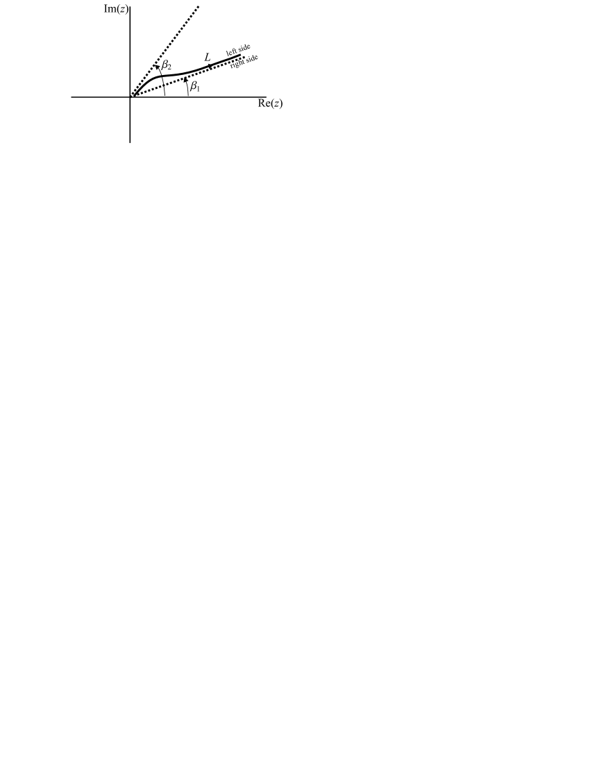
Figure C.1: Contour $L$

Proof.

The proof will consist of three main steps.

Step 1. Consider $L$ as a cut of the $z$ complex plane and define the left and right shores of the cut as in Fig. C.1. Construct a function $y(z)$ analytic in $\mathbb{C}\setminus L$ such that

$$f(z)=y^{\rm r}(z)-y^{\rm l}(z),\qquad z\in L,$$ (C.2)

where $y^{\rm l}$ and $y^{\rm r}$ are the limiting values of $y$ on the left and right shores of $L$ respectively. Such a function is given by the Sokhotsky formula

$$y(z)=\frac{i}{2\pi}\int_{L}\frac{f(z^{\prime})\mathrm{d}z^{\prime}}{z^{\prime}-z}.$$ (C.3)

Step 2. Let $y_{1}(z)$ and $y_{2}(z)$ be the restrictions of $y(z)$ onto the lines ${\rm Arg}(z)=\beta_{1}$ and ${\rm Arg}(z)=\beta_{2}$ respectively. Let $Y_{1}(s)$ and $Y_{2}(s)$ be defined by

$$Y_{1,2}(s)\equiv e^{i\beta_{1,2}}\int\limits_{0}^{\infty}y_{1,2}(\tau e^{i\beta_{1,2}})\exp\{is\tau e^{i\beta_{1,2}}\}\mathrm{d}\tau.$$ (C.4)

The functions $Y_{1}$ and $Y_{2}$ are analytic in the domains where the integrals converge due to the exponential factor, i.e. in the sectors $-\beta_{1}<{\rm Arg}(s)<\pi-\beta_{1}$, $-\beta_{2}<{\rm Arg}(s)<\pi-\beta_{2}$, respectively. These sectors have the common part

$${\mathcal{S}}:\quad-\beta_{1}<{\rm Arg}(s)<\pi-\beta_{2}$$

Due to Cauchy’s theorem and the analyticity property of $y$, for $s\in\mathcal{S}$ we have

$$\int_{L}y^{\rm r}(z)e^{isz}dz=Y_{1}(s),$$ (C.5)

$$\int_{L}y^{\rm l}(z)e^{isz}dz=Y_{2}(s).$$ (C.6)

But by hypothesis,

$$Y_{1}(s)-Y_{2}(s)=F(s)=0\qquad\mbox{ for }s\in\mathcal{S}.$$

This means that we can analytically continue $Y_{1}(s)$ and $Y_{2}(s)$ into a function $Y(s)$ that is analytic on the sector $-\beta_{2}<{\rm Arg}(s)<\pi-\beta_{1}$.

Figure C.2: Contours $\Gamma_{1}$, $\Gamma_{2}$, and $\Gamma_{c}$

Step 3. Let us now introduce the contours $\Gamma_{1}$ and $\Gamma_{2}$ as shown in Fig. C.2. One can reconstruct $y_{1}(z)$ and $y_{2}(z)$ by Mellin transform:

$$y_{1,2}(z)=\frac{1}{2\pi}\int_{\Gamma_{1,2}}Y(s)e^{-isz}\mathrm{d}s.$$ (C.7)

Introduce the contour $\Gamma_{c}$ as shown in Fig. C.2. Note that due to Cauchy’s theorem in (C.7) one can deform $\Gamma_{1}$ or $\Gamma_{2}$ into $\Gamma_{c}$ to get:

$$y_{1,2}(z)=\frac{1}{2\pi}\int_{\Gamma_{c}}Y(s)e^{-isz}\mathrm{d}s.$$ (C.8)

Moreover, remembering that $\beta_{2}-\beta_{1}<\pi$, it is easy to check that the integral of (C.8) defines a function analytic in the sector $\beta_{1}<{\rm Arg}(z)<\beta_{2}$. This function is hence a common analytical continuation of $y_{1}$ and $y_{2}$, implying that $y^{\rm r}(z)=y^{\rm l}(z)$, and finally $f(z)=0$, as required. ∎

It is now possible to formulate and prove the 2D analog of this theorem as follows.

Theorem C.2 (2D uniqueness theorem).

Let $L$ obey conditions of Theorem C.1. Let $f(z_{1},z_{2})$ be a smooth function defined on $L\times L$ and decaying as $|z_{1}|+|z_{2}|\to\infty$. Let us assume that for all $s_{1},s_{2}$ such that $-\beta_{1}<{\rm Arg}(s_{1,2})<\pi-\beta_{2}$, we have

$$F(s_{1},s_{2})\equiv\int_{L}\int_{L}f(z_{1},z_{2})e^{i(s_{1}z_{1}+s_{2}z_{2})}\mathrm{d}z_{1}\,\mathrm{d}z_{2}=0.$$ (C.9)

Then $f(z_{1},z_{2})\equiv 0$.

Proof.

Let us start by defining the function $g(z_{2})$ by

$$g(z_{2}) = \int_{L}f(z_{1},z_{2})e^{is_{1}z_{1}}\,\mathrm{d}z_{1}.$$ (C.10)

The hypothesis (C.9) of the theorem can be rewritten as

$$\int_{L}g(z_{2})e^{is_{2}z_{2}}\,\mathrm{d}z_{2} = 0.$$ (C.11)

The function $g$ can be shown to be smooth and decaying along $L$ and hence, using Theorem C.1, this implies that $g(z_{2})=0$ for all $z_{2}\in L$. Now the integral in (C.10) is equal to zero. We can hence apply Theorem C.1 one last time to prove that $f(z_{1},z_{2})=0$, as required. ∎

References

- [1] A. Sommerfeld. Mathematische Theorie der Diffraction. Mathematische Annalen, 47(2-3):317–374, jun 1896.
- [2] V. M. Babich, M. A. Lyalinov, and V. E. Grikurov. Diffraction Theory: The Sommerfeld-Malyuzhinets Technique. Alpha Science Intl Ltd, 2007.
- [3] D. S. Jones. A simplifying technique in the solution of a class of diffraction problems. Quart. J. Math., 3(1):189–196, 1952.
- [4] N. Wiener and E. Hopf. Über eine Klasse singulärer Integralgleichungen. Akad. d. Wiss., 1931.
- [5] J. B. Lawrie and I. D. Abrahams. A brief historical perspective of the Wiener-Hopf technique. J. Eng. Math., 59(4):351–358, oct 2007.
- [6] B. Noble. Methods Based on the Wiener-Hopf Technique for the Solution of Partial Differential Equations . American Mathematical Society, second edition, 1988.
- [7] J. B. Keller. Geometrical Theory of Diffraction. J. Opt. Soc. Am., 52(2):116–130, 1962.
- [8] V. A. Borovikov and B. Ye. Kinber. Geometrical theory of diffraction. IEE, Electromagnetic Waves Series 37, 1994.
- [9] A. V. Shanin. On wave excitation in a wedge-shaped region. Acoust. Phys., 42(5):696–701, 1996.
- [10] V. G. Daniele and G. Lombardi. Wiener–Hopf solution for impenetrable wedges at skew incidence. IEEE Trans. Antenn. Prop., 54(9):2472–2485, 2006.
- [11] M. Nethercote, R. C. Assier, and I. D. Abrahams. Analytical methods for perfect wedge diffraction: a review. Submitted to Wave Motion, 2018.
- [12] R. Satterwhite. Diffraction by a quarter plane, exact solution, and some numerical results. IEEE Trans. Antennas Propag., 22(3):500–503, 1974.
- [13] A. Erdelyi. Higher Transcendental Functions Volume 3. McGraw-Hill Book Company, 1955.
- [14] L. Klinkenbusch. Electromagnetic scattering by a quarter plane. In Proc. of the 2005 IEEE Antennas and Propagation International Symposium and URSI North American Radio Science Meeting, 2005.
- [15] S. Blume. Spherical-multipole analysis of electromagnetic and acoustical scattering by a semi-infinite elliptic cone. IEEE Antennas Propag. Mag., 38(2):33–44, 1996.
- [16] S. Blume and L. Klinkenbusch. Spherical-multipole analysis in electromagnetics. In D. Werner and R. Mittra, editors, Frontiers in Electromagnetics, chapter 13. IEEE and Wiley, 1999.
- [17] B. V. Budaev and D. B. Bogy. Diffraction of a plane wave by a sector with Dirichlet or Neumann boundary conditions. IEEE Trans. Antennas. Propag., 53(2):711–718, 2005.
- [18] V. P. Smyshlyaev. Diffraction by conical surfaces at high-frequencies. Wave Motion, 12(4):329–339, 1990.
- [19] V. P. Smyshlyaev. The high-frequency diffraction of electromagnetic waves by cones of arbitrary cross sections. SIAM J. Appl. Math., 53(3):670–688, 1993.
- [20] V. M. Babich, D. B. Dement’ev, and B. A. Samokish. On the diffraction of high-frequency waves by a cone of arbitrary shape. Wave Motion, 21(3):203–207, 1995.
- [21] V. M. Babich, V. P. Smyshlyaev, D. B. Dement’ev, and B. A. Samokish. Numerical calculation of the diffraction coefficients for an arbitrary shaped perfectly conducting cone. IEEE Transactions on Antennas and Propagation, 44(5):740, 1996.
- [22] R. C. Assier and N. Peake. Precise description of the different far fields encountered in the problem of diffraction of acoustic waves by a quarter-plane. IMA J. Appl. Math., 77(5):605–625, 2012.
- [23] M. A. Lyalinov. Scattering of acoustic waves by a sector. Wave Motion, 50(4):739–762, jun 2013.
- [24] M. A. Lyalinov. Electromagnetic scattering by a plane angular sector: I. Diffraction coefficients of the spherical wave from the vertex. Wave Motion, 55:10–34, 2015.
- [25] A. V. Shanin. Asymptotics of waves diffracted by a cone and diffraction series on a sphere. J. Math. Sci., 185(4):644–657, 2012.
- [26] V. A. Borovikov. Diffraction by Polygons and Polyhedra. Nauka, Moscow, 1966.
- [27] J. Boersma and J. K. M. Jansen.
- [28] B. A. Hargrave and B. D. Sleeman. The Numerical Solution of Two-parameter Eigenvalue Problems in Ordinary Differential Equations with an Application to the Problem of Diffraction by a Plane Angular Sector. J. Inst. Maths Applics, 14(1):9–22, 1974.
- [29] J. B. Keller. Singularities at the tip of a plane angular sector. J. Math. Phys., 40(2):1087, 1999.
- [30] R. C. Assier, C. Poon, and N. Peake. Spectral study of the Laplace-Beltrami operator arising in the problem of acoustic wave scattering by a quarter-plane. Q. Jl Mech. Appl. Math., 69(3):281–317, 2016.
- [31] M. H. Williams. Diffraction by a finite strip. Q. Jl Mech. Appl. Math., 35:103–124, 1982.
- [32] R. V. Craster, A. V. Shanin, and E. M. Doubravsky. Embedding formulae in diffraction theory. Proc. R. Soc. A, 459(2038):2475–2496, 2003.
- [33] A. V. Shanin. Modified Smyshlyaev’s formulae for the problem of diffraction of a plane wave by an ideal quarter-plane. Wave Motion, 41(1):79–93, 2005.
- [34] A. V. Shanin. Coordinate equations for a problem on a sphere with a cut associated with diffraction by an ideal quarter-plane. Q. Jl Mech. Appl. Math., 58(2):289–308, 2005.
- [35] R. C. Assier and N. Peake. On the diffraction of acoustic waves by a quarter-plane. Wave Motion, 49(1):64–82, 2012.
- [36] R. C. Assier. On the diffraction of acoustic waves by a quarter-plane. Phd thesis, University of Cambridge, 2012.
- [37] V. Y. Valyaev and A. V. Shanin. Embedding formulae for Laplace-Beltrami problems on the sphere with a cut. Wave Motion, 49(1):83–92, 2012.
- [38] E. Meister and F-O. Speck. A Contribution to the Quarter-Plane in Diffraction Theory*. J. Math. Anal. Appl., 130:223–236, 1988.
- [39] V.A. Kakichev. Boundary-value problems of linear matching of functions holomorphic in bicylindrical domains. Doklady Akademii nauk SSSR (in Russian), 178(5):1003–1006, 1968.
- [40] V.S. Rabinovich. Multidimensional Wiener–Hopf equation for cones. Theory of functions, functional analysis, and their applications (in Russian), (5):59–67, 1967.
- [41] N.I. Moraru. Cases of the Wiener–Hopf equation on a quadrant of the plane. Differential equations (in Russian), 5(8):1445–1457, 1969.
- [42] V. B. Vasil’ev. Wave Factorization of Elliptic Symbols: Theory and Applications. Springer, 2000.
- [43] J. Radlow. Diffraction by a quarter-plane. Arch. Ration. Mech. Anal., 8(2):139–158, 1961.
- [44] J. Radlow. Note on the diffraction at a corner. Arch. Ration. Mech. Anal., 19:62–70, 1965.
- [45] E. Meister. Some solved and unsolved canonical problems of diffraction theory. Lect. Notes Math., 1285:320–336, 1987.
- [46] M. Albani. On Radlow’s quarter-plane diffraction solution. Radio Sci., 42(6):1–10, oct 2007.
- [47] R. C. Assier and I. D. Abrahams. A surprising observation in the quarter-plane problem. to be submitted, 2018.
- [48] B. V. Shabat. Introduction to complex analysis Part II. Functions of several variables. American Mathematical Society, 1992.
- [49] G. M. Khenkin and A. G. Vitushkin. Several Complex Variables II: Function Theory in Classical Domains, Complex Potential Theory. Springer, 1994.