Accurate radial velocity and metallicity of the Large Magellanic Cloud old globular clusters NGC 1928 and NGC 1939

Abstract

We present results obtained from spectroscopic observations of red giants located in the fields of the Large Magellanic Cloud (LMC) globular clusters (GCs) NGC 1928 and NGC 1939. We used the GMOS and AAOmega+2dF spectrographs to obtain spectra centred on the Ca II triplet, from which we derived individual radial velocities (RVs) and metallicities. From cluster members we derived mean RVs of RV${}_{\rm NGC\,1928}=249.58\pm$4.65 km/s and RV${}_{\rm NGC\,1939}=258.85\pm$2.08 km/s, and mean metallicities of [Fe/H]${}_{\rm NGC\,1928}=-1.30\pm$0.15 dex and [Fe/H]${}_{\rm NGC\,1939}=-2.00\pm$0.15 dex. We found that both GCs have RVs and positions consistent with being part of the LMC disc, so that we rule out any possible origin but that in the same galaxy. By computing the best solution of a disc that fully contains each GC, we obtained circular velocities for the 15 known LMC GCs. We found that 11/15 of the GCs share the LMC rotation derived from $HST$ and $Gaia$ DR2 proper motions. This outcome reveals that the LMC disc existed since the very early epoch of the galaxy formation and experienced the steep relatively fast chemical enrichment shown by its GC metallicities. The four remaining GCs turned out to have circular velocities not compatible with an in situ cluster formation, but rather with being stripped from the SMC.

1 Introduction

Only fifteen old GCs (GCs, ages $\ga$ 12 Gyr) are known to survive in the Large Magellanic Cloud (LMC) (Piatti & Geisler, 2013), of which NGC 1928 and NGC 1939 have only recently been added by Dutra et al. (1999, hereafter D99). Their first colour-magnitude diagrams come from $HST$ photometry (Mackey & Gilmore, 2004), confirming their old ages. As far as we are aware, neither NGC 1928 nor NGC 1939 have published accurate metallicity or radial velocity (RV) measurements.

The orbital motions of LMC ancient GCs are satisfactorily described by a disc-like rotation with no GC appearing to have halo kinematics (Sharma et al., 2010). Schommer et al. (1992) found that these clusters form a disc that agrees with the parameters of the optical isophotes and inner H I rotation curve. There are some other galaxies that appear to have GC systems with kinematic properties related to the H I discs (e.g. Olsen et al., 2004), which might suggest a benign evolutionary history, such as might be expected if the LMC has evolved in a low density environment.

However, the destruction of a GC system that is on a coplanar orbit about a larger galaxy could also produce such a disc-like rotation geometry (Leaman et al., 2013). Furthermore, van den Bergh (2004) showed that the possibility that the LMC old GCs formed in a pressure-supported halo, rather than in a rotating disc, should not be discarded. In this sense, Carrera et al. (2008) argued that the lack of evidence of such a hot stellar halo in the LMC is related to a low contrast of the halo population with respect to that of the disc, particularly at the innermost galactocentric radii where NGC 1928 and NGC 1939 are located. On the other hand, Carpintero et al. (2013) modelled the dynamical interaction between the Small Magellanic Cloud (SMC) and the LMC, and found that at least some of the oldest clusters observed in the LMC could have originated in the SMC.

The LMC old GCs have also been compared to those of the Milky Way (MW). Brocato et al. (1996), Mucciarelli et al. (2010) and Wagner-Kaiser et al. (2017), among othes, showed that the old LMC GCs resemble the MW ones in age and in many chemical abundance patterns. In contrast, Johnson et al. (2006) found that many of the abundances in the LMC old GCs are distinct from those observed in the MW, while Piatti & Geisler (2013) suggested that the most likely explanation for the difference between the old GC and field star age-metallcity relationships is a very rapid early chemical enrichment traced by the very visible old GCs. Indeed, the integrated spectroscopic metallicities obtained by Dutra et al. (1999) suggest that NGC 1928 is one of the most metal-rich ([Fe/H] $\sim$ -1.2 dex) old GCs, whereas NGC 1939 one of the most metal-poor ([Fe/H] $\sim$ -2.0 dex) old GCs.

In Section 2 we describe the spectroscopic observations performed with the aim of deriving for the first time accurate mean cluster RVs (Section 3) and metallicities (Section 4). These quantities are considered in Section 5 to investigate whether NGC 1928 and NGC 1939 have been born in the LMC disc, or have other origins. Finally, a summary of the results is presented in Section 6.

2 Observational data sets

We carried out spectroscopic observations centred on the Ca II infrared triplet ($\sim$ 8500 Å) of red giant stars located in the fields of NGC 1928 and 1939. Most of the targets were selected from the $HST$ photometric data set of Mackey & Gilmore (2004), bearing in mind their loci in the cluster colour-magnitude diagrams (CMDs). Because of the relatively small cluster angular sizes ($\la$ 1 arcmin) and their high crowding, many cluster red giants were discarded. For this reason, we considered some few other relatively bright red giant stars (4 in NGC 1928 and 1 in NGC 1939) without $HST$ photometry. Fig. 1 illustrates the positions of the selected targets in the cluster fields and CMDs, respectively. In the case of NGC 1939, we have also available $CT_{1}$ Washington photometry (Piatti, 2017), from which we built the cluster CMD of Fig. 2.

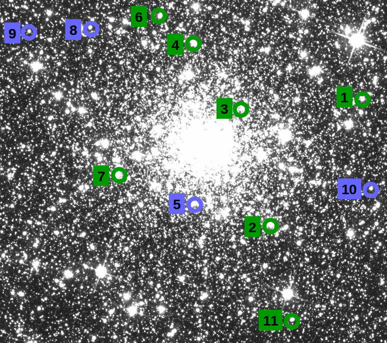
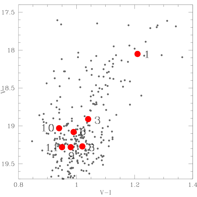
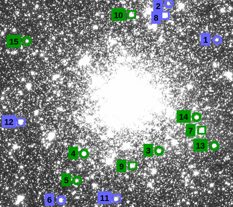
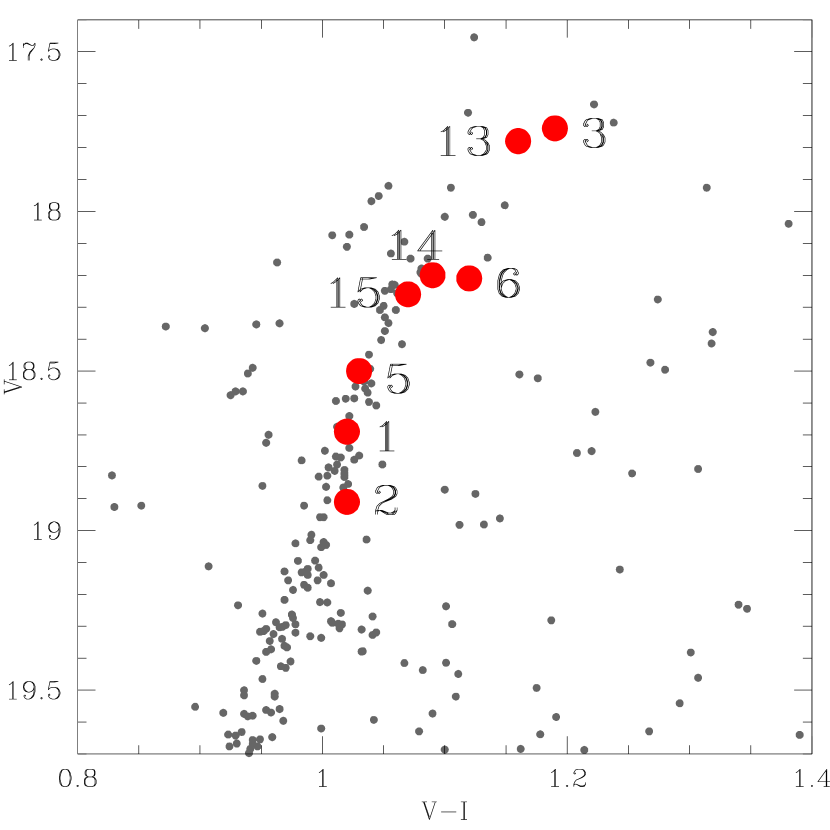
Figure 1: 40$\arcsec$$\times$40$\arcsec$ publicly available $F555W$ images centred on NGC 1928 (top) and on NGC 1939 (bottom) with the selected targets labelled with the ID numbers of Table 1. Green and blue symbols represent member and non-member stars, respectively (see Table 2); while circles and boxes correspond to stars observed with GMOS and AAOmega+2dF, respectively. The right-hand panels show the cluster CMDs for the respective image areas, where selected stars with available Mackey & Gilmore (2004)’s photometry are higlighted with red filled circles.

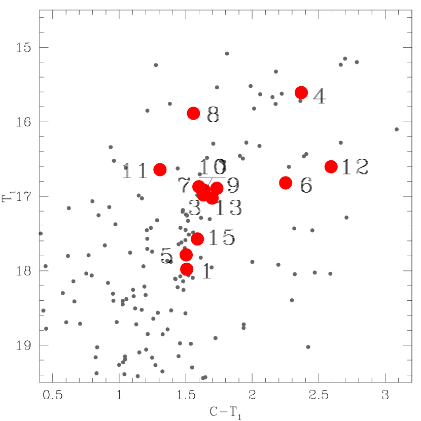
Figure 2: NGC 1939’s $CT_{1}$ CMD for stars located in the same area as in Fig. 1, taken from Piatti (2017). Selected stars are highlighted with filled red circles.

2.1 Gemini South Observatory: GMOS spectra

We carried out spectroscopic observations of stars in the field of NGC 1928 and NGC 1939 using the Gemini Multi-Object Spectrograph (GMOS) of Gemini South observatory during the nights of October 21 and 25, 2017, through programmes GS-2017B-Q-23 and GS-2017B-Q-71 (PI: Piatti), respectively. For each star cluster, we took four consecutive exposures of 900 sec for a single mask, as well as CuAr arcs and flats before and after the individual science exposures in order to secure a stable wavelength calibration. The total integration time for the science targets was 3600 sec. We used the R831 grating and the OG515 (> 520 nm) filter, combined with a mask of 1.0 arcsec wide slits placed on the target stars, which gave a spectral sampling of $\sim$ 0.75Å per pixel with the 2$\times$2 CCD binning configuration. We observed 11 and 9 science target stars in the field of NGC 1928 and NGC 1939, respectively.

We reduced the spectra following the standard GMOS data reduction procedure using the IRAF.gemini.gmos package. The wavelength calibration was derived using the gswavelength task, which compares the observed spectra with GCAL arc lamp data, and a wavelength solution was derived with a rms less than 0.20Å. We also used sky OH emission lines to further constrain the wavelength calibration and applied small offsets of about 0.3$-$0.5Å  to the science spectra. The final dispersion of our data turned out to be 26.47 km/sec per pixel and the S/N ratio of the resulting spectra ranges from 30 up to 100, measured using the local continuum of the Ca II triplet. Fig. 3 illustrates spectra of some science targets.

Figure 3: Normalised spectra of some observed stars.

2.2 Anglo-Australian Telescope: AAOmega+2dF spectra

We observed the region around ($\alpha$, $\delta$) = (5:24, $-$68:48) with the AAOmega spectrograph and 2dF fibre positioner at the 3.9m AAT on 2017 December 10–11, as part of a followup program intended to identify the most metal-poor red giants in the LMC (Emptage et al., in preparation). The fibre positions were chosen to optimise overlap with the targets in Cole et al. (2005) and Van der Swaelmen et al. (2013) in order to provide metallicity cross-calibration. NGC 1939 is not far from the field centre, so 6 fibres were assigned to red giants within 3^′ of the cluster, over two configurations of the fibre plate. No fibers were assigned to stars in the vicinity of NGC 1928, a sparser cluster farther from the 2dF field centre.

On 10 December, the field was observed for 3$\times$1800 s in 1$\aas@@fstack{\prime\prime}$6 seeing, and the following night a second fibre configuration was observed for 3$\times$1200 s in 1$\aas@@fstack{\prime\prime}$4 seeing. The red arm of the spectrograph was employed with the 1700D grating, centred on $\lambda_{c}$ = 8600 Å, for a dispersion of $\approx$0.24 Å per pixel, and a resolution R $\approx$11,000, depending on the position of the fibre image on the CCD. Arc and fibre flat exposures were taken immediately prior to each set of three science exposures.

The data were reduced using the standard 2dfdr data reduction package, which tunes the extraction parameters to optimise the signal to noise, producing wavelength-calibrated, sky-subtracted spectra. We obtained typical SNR values in the continuum of $\approx$15–50 depending on target I magnitude and fibre centring accuracy. Continuum normalisation was performed using the IRAF task continuum, with a sixth-order cubic spline fit and rejection of unusually low points, which are assumed to be photospheric lines. The spectra were not flux-calibrated, as we intend only to measure equivalent widths and radial velocities.

3 Radial velocity measurements

3.1 GMOS spectra

We measured RVs by cross-correlating the observed spectra and synthetic ones taken from the PHOENIX library (Husser et al., 2013). The synthetic spectra library covers the wavelength range 500 $-$ 55000 Å and provides a wide coverage in effective temperatures ($T_{\textrm{eff}}$ $\sim 2300-12000\,^{\rm o}$K), surface gravities (log ($g$) $\sim 0.0-6.0$ dex) and metallicities ([Fe/H] $\sim-4.0-+1.0$ dex). We selected templates with $T_{\textrm{eff}}$ in the range $4000-5500\,^{\rm o}$K and log ($g$) between $1.5-3.0$ dex, which correspond to giant stars with MK types $\sim$ G0$-$K4. In the case of NGC 1928, we restricted the templates to those with [Fe/H]$=-1.0$ dex, while for NGC 1939 we employed those with [Fe/H]$=-2.0$ dex (see Section 4). In both cases, we selected 224 templates and checked that the restriction in metallicity already has a negligible impact on the RV estimates, since variations of 1.0 dex in [Fe/H] resulted in a change of $\sim$ 1 km/s in the derived RV (see also Fig. 4).

The observed spectra were continuum normalised before the cross-correlation procedure and the synthetic templates had their spectral resolution degraded to match the resolution of our science spectra. We employed the transformation equations of Ciddor (1996) to convert the wavelength grids from vacuum ($\lambda_{\textrm{vac}}$) to air wavelengths ($\lambda_{\textrm{air}}$; see also Section 3.2 of Angelo et al. (2017) for more details). Spectral fluxes ($F_{\lambda}^{\textrm{vac}}=\frac{dE_{\lambda}}{dt\,d\lambda_{\textrm{vac}}\,d\textrm{Area}}$) were also converted from vacuum to air values through the expression:

$$F_{\lambda}^{\textrm{air}}=\frac{dE_{\lambda}}{dt\,d\lambda_{\textrm{air}}\,d\textrm{Area}}=F_{\lambda}^{\textrm{vac}}\left(\frac{d\lambda_{\textrm{vac}}}{d\lambda_{\textrm{air}}}\right)$$ (1)

Each observed spectrum was cross-correlated against the whole selected synthetic template sample by making use of the IRAF.fxcor task, which implements the algorithm described in Tonry & Davis (1979) for the construction of the cross-correlation function (CCF) of each object - template pair of spectra. Besides the RV estimates, fxcor returns the CCF normalised peak ($h$) $-$ an indicator of the degree of similarity between the correlated spectra $-$ and the Tonry & Davis ratio (TDR) defined as TDR$=h/(\sqrt{2}\sigma_{a})$, where $\sigma_{a}$ is root mean square of the CCF antisymmetric component.

For each object spectrum we assigned the RV value resulting from the cross-correlation with the highest $h$ value, which was in all cases greater than 0.8. We finally carried out the respective heliocentric corrections. Table 1 lists the resulting RVs with their respective uncertainties, while Fig. 4 illustrates the cross-correlation procedure.

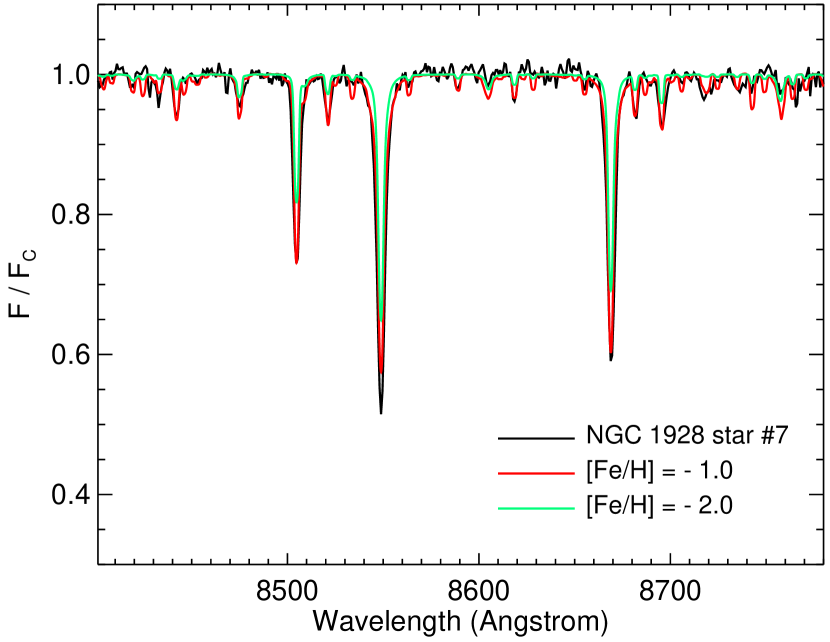
Figure 4: Continuum normalised spectrum of star #7 of NGC 1928 (black lines) and the best fitted synthetic template spectra for [Fe/H]$=-1.0$ dex (red line) and $-2.0$ dex (green line), respectively.

3.2 AAOmega+2dF spectra

We measured radial velocities by Fourier cross-correlation between the target star spectra and a set of templates obtained at the same resolution and signal-to-noise ratio. The templates were LMC field red giants observed by Cole et al. (2005), with metallicities from $-1\lesssim$ [M/H] $\lesssim$ $-2$, and radial velocities between 200–300 km/s. Relative velocities for each star compared to each template in turn were calculated using fxcor in IRAF, and converted to a heliocentric frame. The radial velocities based on each template were averaged together, weighted by the cross-correlation peak height. The uncertainty in the resulting average velocities is on the order of $\pm$3 km/s, and is dominated by scatter between the various templates. Therefore the line of sight velocity dispersion of the field stars is highly resolved by these measurements, but cluster is expected to be unresolved.

Table 1: Positions, radial velocities, Ca II triplet lines equivalent widths and metallicities of the selected targets.

ID	Instrument	R.A.	Dec.	S/N	RV	W8498	W8542	W8662	[Fe/H]
		(deg)	(deg)		(km/s)	(Å)	(Å)	(Å)	(dex)
NGC 1928-1	GMOS	80.217297	-69.475896	71.3	250.29$\pm$3.03	1.024$\pm$0.010	2.516$\pm$0.086	1.724$\pm$0.023	-1.35$\pm$0.13
NGC 1928-2	GMOS	80.230389	-69.481931	102.5	245.02$\pm$2.77	1.259$\pm$0.090	2.606$\pm$0.035	1.960$\pm$0.063	—
NGC 1928-3	GMOS	80.234166	-69.476247	33.1	238.61$\pm$6.92	0.983$\pm$0.040	1.963$\pm$0.070	1.847$\pm$0.093	-1.32$\pm$0.17
NGC 1928-4	GMOS	80.240765	-69.472867	66.7	268.80$\pm$2.52	1.832$\pm$0.112	3.567$\pm$0.106	2.207$\pm$0.107	—
NGC 1928-5	GMOS	80.241292	-69.480756	64.7	286.96$\pm$3.37	1.863$\pm$0.105	3.510$\pm$0.160	2.247$\pm$0.048	—
NGC 1928-6	GMOS	80.245312	-69.471593	49.2	261.24$\pm$5.92	0.816$\pm$0.036	2.284$\pm$0.052	1.55$\pm$0.056	-1.33$\pm$0.15
NGC 1928-7	GMOS	80.251698	-69.479367	86.3	251.72$\pm$3.08	1.089$\pm$0.033	2.678$\pm$0.071	2.039$\pm$0.048	—
NGC 1928-8	GMOS	80.255200	-69.472097	46.3	216.78$\pm$6.25	1.021$\pm$0.061	2.875$\pm$0.139	2.329$\pm$0.140	-0.71$\pm$0.24
NGC 1928-9	GMOS	80.263638	-69.472226	53.6	214.11$\pm$3.81	0.970$\pm$0.032	2.780$\pm$0.120	1.875$\pm$0.094	-0.93$\pm$0.20
NGC 1928-10	GMOS	80.216320	-69.480298	47.7	280.37$\pm$5.58	1.286$\pm$0.080	3.065$\pm$0.114	2.316$\pm$0.084	-0.61$\pm$0.23
NGC 1928-11	GMOS	80.227749	-69.486631	29.0	231.37$\pm$8.27	0.950$\pm$0.100	1.958$\pm$0.157	1.631$\pm$0.040	-1.33$\pm$0.21
NGC 1939-1	GMOS	80.339326	-69.944931	56.6	279.94$\pm$6.76	0.630$\pm$0.095	1.351$\pm$0.026	1.274$\pm$0.035	-1.95$\pm$0.13
NGC 1939-2	GMOS	80.350991	-69.942040	39.6	258.18$\pm$4.92	1.599$\pm$0.133	3.203$\pm$0.220	2.486$\pm$0.123	-0.41$\pm$0.30
NGC 1939-3	GMOS	80.352639	-69.954109	83.1	261.36$\pm$3.69	0.688$\pm$0.046	1.584$\pm$0.030	1.351$\pm$0.042	-2.05$\pm$0.10
NGC 1939-4	GMOS	80.370202	-69.954369	22.1	260.40$\pm$2.93	0.932$\pm$0.013	2.139$\pm$0.012	1.577$\pm$0.068	-2.00$\pm$0.09
NGC 1939-5	GMOS	80.371903	-69.956597	40.5	241.33$\pm$13.40	0.711$\pm$0.060	1.576$\pm$0.044	0.899$\pm$0.030	-2.02$\pm$0.12
NGC 1939-6	GMOS	80.375680	-69.958244	49.9	250.52$\pm$3.92	1.589$\pm$0.050	3.528$\pm$0.095	2.634$\pm$0.051	-0.41$\pm$0.19
NGC 1939-7	AAO+2dF	80.342251	-69.952236	25.3	259.90$\pm$2.50	0.900$\pm$0.100	1.176$\pm$0.118	1.384$\pm$0.138	-2.14$\pm$0.15
NGC 1939-8	AAO+2dF	80.351829	-69.943060	26.6	282.50$\pm$3.40	0.800$\pm$0.100	2.348$\pm$0.235	2.502$\pm$0.250	-1.57$\pm$0.24
NGC 1939-9	AAO+2dF	80.358841	-69.955288	24.9	259.90$\pm$2.80	0.809$\pm$0.081	2.048$\pm$0.205	1.131$\pm$0.113	-1.94$\pm$0.21
NGC 1939-10	AAO+2dF	80.359225	-69.943083	19.2	259.60$\pm$2.80	0.569$\pm$0.057	2.067$\pm$0.207	1.224$\pm$0.122	-1.98$\pm$0.20
NGC 1939-11	AAO+2dF	80.362350	-69.957974	13.8	257.90$\pm$3.50	1.400$\pm$0.100	4.016$\pm$0.402	2.416$\pm$0.242	-0.60$\pm$0.35
NGC 1939-12	AAO+2dF	80.385450	-69.951819	25.0	270.20$\pm$2.80	1.495$\pm$0.150	3.880$\pm$0.388	2.950$\pm$0.295	-0.44$\pm$0.42
NGC 1939-13	GMOS	80.339554	-69.953529	76.8	268.59$\pm$3.61	0.681$\pm$0.040	1.747$\pm$0.046	1.445$\pm$0.030	-1.95$\pm$0.11
NGC 1939-14	GMOS	80.343735	-69.951279	40.3	253.30$\pm$11.01	0.502$\pm$0.078	1.573$\pm$0.055	1.093$\pm$0.030	-1.85$\pm$0.14
NGC 1939-15	GMOS	80.384301	-69.945343	64.0	264.30$\pm$3.19	0.450$\pm$0.111	1.743$\pm$0.041	1.401$\pm$0.033	-1.93$\pm$0.14

4 Overall metallicity estimates

4.1 GMOS spectra

Equivalent widths of the CaII infrared triplet lines were measured from the normalised spectra using the splot package within IRAF. Their resulting average values and the respective uncertainties are listed in Table 1. The latter were estimated by computing equivalent widths using different continua, bearing in mind the presence of TiO bands and the spectra S/N ratio. We then overplotted the sum of the equivalent widths of the three CaII lines ($\Sigma$W(CaII)) in the $\Sigma$W(CaII) versus $V-V_{\rm HB}$ plane, that has been calibrated in terms of metallicity (see, e.g., Cole et al., 2004). In that diagram $V_{\rm HB}$ refers to the mean magnitude of the cluster horizontal branch. For NGC 1928 and NGC 1939 we adopted the individual $V$ magnitudes of the selected stars and $V_{\rm HB}$ $=19.3$ mag, taken from Mackey & Gilmore (2004) (see also Fig. 1). We also took advantage of the Washington photometry of Piatti (2017) (see also Fig. 2) to convert $T_{1}$ magnitudes of the selected stars into $V$ magnitudes $-$ for those stars without $HST$ $V$ mags $-$ using the theoretical red giant branches computed by Bressan et al. (2012), and the cluster reddening and distance moduli derived by Mackey & Gilmore (2004). Fig. 5 shows the resulting plots, where we included iso-abundance lines according to eq. (5) of Cole et al. (2004) for $\beta=0.64$ Å/mag (Rutledge et al., 1997), while the last column of Table 1 lists the interpolated [Fe/H] values. The errors were calculated by propagating those of the coefficients in eq. (5) (Cole et al., 2004), $\sigma$($\beta$) (Rutledge et al., 1997), the $HST$ (Mackey & Gilmore, 2004) and Washington (Piatti, 2017) photometric errors and $\sigma(\Sigma$W(CaII)), respectively.

4.2 AAOmega+2dF spectra

Equivalent widths of the Ca II triplet lines were measured using the program EW, originally written by G.S. da Costa and used by Cole et al. (2005) and many others (e.g. Da Costa, 2016). The lines were fit by a sum of Gaussian plus Lorentzian profiles, constrained to have a common centroid. The metallicities were measured as for the GMOS stars, described above. Because of the lower SNR, we tested the results against the method of Starkenburg et al. (2010), using only the two strongest lines of the Ca triplet; no significant differences were found within the errorbars. The total error on metallicity is dominated by systematic effects (e.g., possible differences in detailed abundance ratios between the target stars and those used to form the calibration sample) rather than random error from photon noise. For the field stars in the vicinity of NGC 1939 in common with Cole et al. (2005), comparing the equivalent widths measured in the 2017 AAOmega spectra shows an average difference of $\sum$W_AAO-VLT = 0.06 $\pm$0.38 Å, highly consistent with no systematic offset.

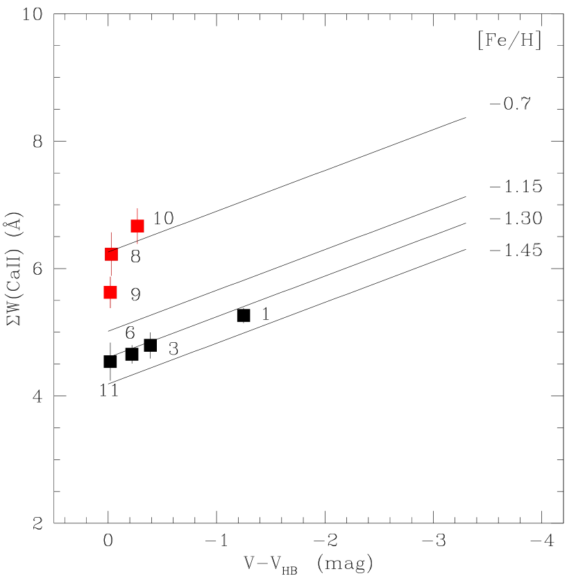
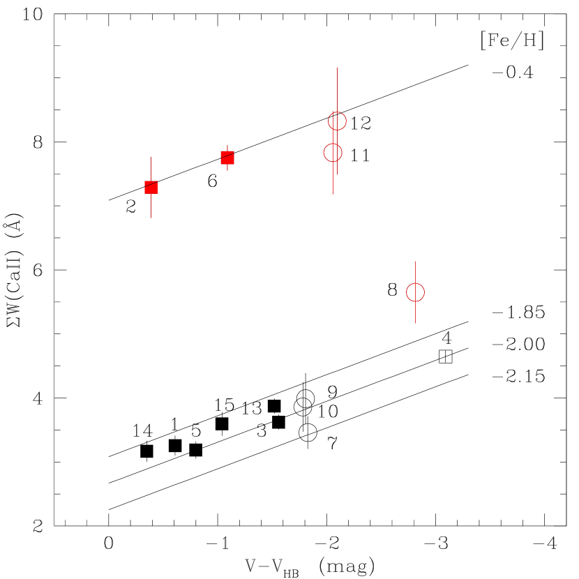
Figure 5: Sum of the CaII triplet line equivalent widths as a function of $V-V_{HB}$ for stars observed in the fields of NGC 1928 (left) and NGC 1939 (right). Black and red symbols represent cluster and field stars, respectively, while boxes and circles correspond to GMOS and AAOmega+2dF spectra, respectively. Filled and open symbols refers to stars with $HST$ $V$ mag taken from Mackey & Gilmore (2004) and those with only Washington $T_{1}$ mags of Piatti (2017) converted into $V$ ones (see text for details). Errorbars are also drawn. Iso-abundance lines derived by Cole et al. (2004) for some [Fe/H] values are also depicted.

5 Analysis and discussion

We first assigned to the observed stars cluster membership probabilities according to three different criteria, namely: the position of the stars in the cluster CMDs, the dispersion of their RV values and that for their [Fe/H] values, respectively. For NGC 1928, we previously discarded stars #8 and 9, which fall outside the cluster radius recently estimated by Piatti & Mackey (2018, 31.6$\pm$7.3 arcsec) from a radial profile that reaches out to $\sim$ 4 times the cluster’s tidal radius.

By looking at the cluster CMDs (Figs. 1 and 2) we considered possible members any star located along the cluster red giant branches, within the observed spread of those sequences. We included the results of our assessment in column 2 of Table 2. Note that this criterion could lead us to conclude on the cluster membership of any star that belongs to the LMC star field, because of the superposition with LMC field features. This is the case, for instance, of the LMC field red clump.

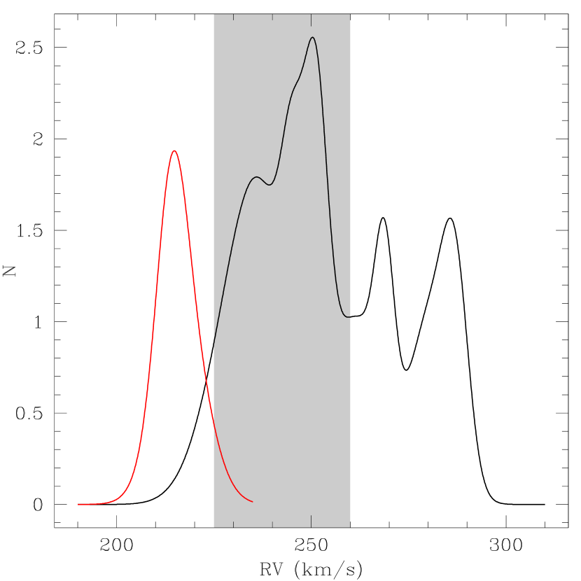
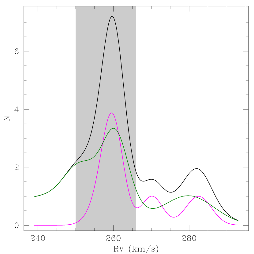
Figure 6: RV distribution functions for stars observed in the field of NGC 1928 (left) and NGC 1939 (right) are drawn with a solid black line. The red line in the left panel corresponds to the RV distribution of non-member stars #8 and 9, while the green and magenta lines in the right panel refer to the RV distributions obtained from stars observed with GMOS and AAOmega+2dF, respectively. The shadowed regions correspond to the cluster RV ranges.

We then built RV distribution functions by summing all the individual RV values, each of them represented by a Gaussian with centre and $\sigma$ equal to the mean RV value and the associated error, respectively (see Table 1). Every Gaussian was assigned the same amplitude. The resulting RV distributions are shown in Fig. 6, where the cluster RV ranges can be clearly identified from the FWHM of the primary peak (shadowed regions). In NGC 1928’s panel, we intentionally included stars #8 and 9 (red curve), thus confirming that they are probably non-members. In NGC 1939, we also plotted the RV distributions obtained from using only stars observed with GMOS (green curve) and with AAOmega+2dF (magenta curve), respectively. As can be seen, there is a negligible shift between both RV scales, so that we summed them to produce the overall RV distribution (black curve). Table 2 lists the RV membership status assigned to each star on the basis of whether its RV falls within the shadowed regions.

As for the metallicity membership probability, we visually inspected Fig. 5, in which star sequences along a constant [Fe/H] value can be recognised, with some dispersion. For instance, the $\Sigma$W(CaII) versus $V-V_{\rm HB}$ diagram for NGC 1928 (left panel) shows stars #8 and 9 $-$ initially discarded because they fall outside the cluster radius $-$ and #10 at a very distinguishable higher metallicity level. These stars have also RVs quite different from those of the observed cluster members. For the remaining stars, we do not have any argument as to deny them cluster membership. In the case of NGC 1939 (right panel), the observed more metal-poor sequence contains more than three times the number of stars in the more metal-rich sequence ([Fe/H] $\sim-0.4$ dex), so that we concluded that the former corresponds to that of the cluster. Note that the separation between both sequences is similar for $\Sigma$W(CaII) obtained from GMOS and AAOmega+2dF spectra, respectively. According to Cole et al. (2005, see their figure 6), the derived [Fe/H] values for the observed stars meant to be LMC field stars (red symbols) are in excellent agreement with the bulk of metallicity values of LMC bar field giants.

The final membership status of each star is listed in the last column of Table 2. Only stars #1 and 6 observed in the field of NGC 1939 have RV memberships different from those adopted using separately their positions in the cluster CMDs and their metallicities, respectively. Nevertheless, we rely on the possibility that LMC field stars can have either RVs or metal-contents similar to that of the cluster. This is not the case of the field giant #2 observed also along the line-of-sight of NGC 1939, whose $V$ magnitude and $V-I$ colour place it superimposed on the cluster red giant branch (see Fig. 1). For the remaining stars observed in both cluster fields, the three membership criteria totally agree.

We finally used the RV and [Fe/H] values of all cluster members to derive the mean cluster RVs and metallicities by employing a maximum likelihood approach. The relevance lies in accounting for individual star measurements, which could artificially inflate the dispersion if ignored. We optimized the probability $\mathcal{L}$ that a given ensemble of stars with velocities RV_i and errors $\sigma_{i}$ are drawn from a population with mean RV $<$$RV$$>$ and dispersion W (e.g., Pryor & Meylan, 1993; Walker et al., 2006), as follows:

$$\small\mathcal{L}\,=\,\prod_{i=1}^{N}\,\left(\,2\pi\,(\sigma_{i}^{2}+W^{2}\,)\right)^{-\frac{1}{2}}\,\exp\left(-\frac{(RV_{i}\,-<RV>)^{2}}{\sigma_{i}^{2}+W^{2}}\right).$$ (2)

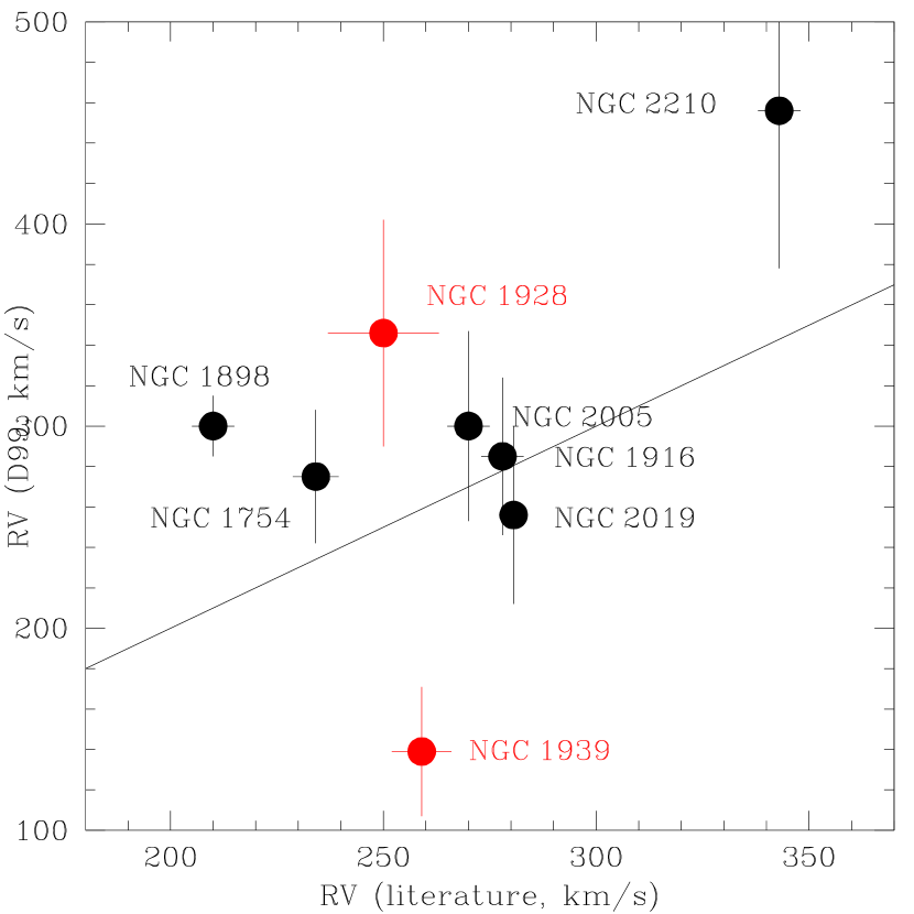
Figure 7: Comparison of LMC GC RVs derived by D99 with those available in the literature (see Table 3).

where the errors on the mean and dispersion were computed from the respective covariance matrices. We obtained for NGC 1928, $<$RV${}_{\rm NGC\,1928}>=249.58\pm$4.65 km/s and $<$[Fe/H]${}_{\rm NGC\,1928}>=-1.30\pm$0.15 dex, while for NGC 1939 the mean values turned out to be $<$RV${}_{\rm NGC\,1939}>=258.85\pm$2.08 km/s and $<$[Fe/H]${}_{\rm NGC\,1939}>=-2.00\pm$0.15 dex. We compared our mean cluster RVs with those previously obtained by D99, who mentioned that their integrated spectra were not particularly suitable for accurate velocity measurements. Fig. 7 shows the results, where other LMC GCs with RV estimates available in the literature were added.

One of the diagnostic diagrams most frequently used to assess whether a cluster belongs to the LMC disc is that which shows the relationship between position angles (PAs) and RVs (Schommer et al., 1992; Grocholski et al., 2006; Sharma et al., 2010; van der Marel et al., 2002; van der Marel & Kallivayalil, 2014) for a disc-like rotation geometry. We here followed the recipe used by Schommer et al. (1992), who converted the observed heliocentric cluster RVs to Galactocentric RVs through eq.(4) in Feitzinger & Weiss (1979). We computed cluster PAs by adopting the LMC disc central coordinates and their uncertainties obtained by van der Marel & Kallivayalil (2014) from $HST$ average proper motion measurements for stars in 22 fields. Fig. 8 shows the disc solution derived for those $HST$ proper motions (Table 1 in van der Marel & Kallivayalil, 2014) represented with a solid line, as well as those considering the uncertainties in the LMC disc line-of-sight systemic velocity, circular velocity and PA of the line-of-nodes and the derived velocity dispersion (dotted lines). As can be seen, NGC 1928 and 1939 are placed within the fringes of the LMC disc at 1$\sigma$ confidence, similarly to many of the remaining 13 GCs included in the figure for comparison purposes.

Therefore, assuming that both GCs belong to the LMC disc, we then sought for the best disc solutions for their respective RVs and position in the galaxy, i.e., we looked for the circular velocity ($v_{\rm rot}$) and PA of the line-of-nodes (PA_LOS) of the discs that fully contain them. To do that, we used a grid of $v_{\rm rot}$ and PA_LOS values to evaluate eq.(1) of Schommer et al. (1992) for the cluster PAs and their uncertainties, and then to find the most likely pair ($v_{\rm rot}$,PA_LOS) that minimizes by $\chi^{2}$ the difference between the cluster RVs with their errors and those calculated above. We used a grid of $v_{\rm rot}$ from 0.0 up to 200.0 km/s in steps of 1.0 km/s, and a range of PA_LOS from 0.0 up to 360.0 degrees in steps of 1.0 degree. For NGC 1928, the most suitable disc turned out to be that with $v_{\rm rot}=45.0\pm$10.0 km/s and PA${}_{\rm LOS}=85.0\pm$10.0 degrees, while the resulting one for NGC 1939 is that with $v_{\rm rot}=35.0\pm$10.0 km/s and PA${}_{\rm LOS}=130.0\pm$10.0 degrees. For comparison purposes, we also computed $v_{\rm rot}$ and PA_LOS values for the remaining LMC GCs (see Table 3).

Fig. 9 depicts the resulting $v_{\rm rot}$ values as a function of the deprojected distances ($r$, see Table 3). The latter were computed using the LMC disc fitted by van der Marel & Kallivayalil (2014) from $HST$ proper motions in 22 fields, whose rotation curve is represented in the figure by a solid black line. The rotation curves obtained from line-of-sight (LOS) velocities of young and old stars (van der Marel & Kallivayalil, 2014) are drawn with red and blue solid lines, respectively, and that from $Gaia$ DR2 proper motions (Vasiliev, 2018) with a magenta line. The figure reveals that NGC 1928 and 1939 very well match the $HST$ proper motion rotation curve, as also do many other GCs. Reticulum ($r=$ 10.2 kpc, $v_{\rm rot}=$35 km/s) seems to rotate slower than the old stellar population LOS rotation curve, while NGC 1835, 1898 and 2210 ($v_{\rm rot}>$ 100 km/s) are high circular velocity objects.

Because the disc-like rotation geometry is shared by most the GCs (age $\ga$ 12 Gyr), we infer that the LMC disc had to exist since the early epoch of the galaxy formation, not only as an structure in itself but also from a dynamical point of view with a non-negligible angular momentum. The GCs that follow such rotation pattern span the entire metallicity range of all the GCs in the galaxy (-2.0 $\la$ [Fe/H] (dex) $\la$ -1.3, see also Table 3), so that the LMC disc had also to experience a similar chemical enrichment within $\sim$ 3 Gyr of its GC formation (12 $\la$ age (Gyr) $\la$ 14, Piatti et al., 2009; Wagner-Kaiser et al., 2018). Furthermore, because of the lack of a clear metallicity gradient among the disc GCs, we conclude that the whole disc - except possibly its very outskirts ($r>$ 15 kpc) - has been chemically evolved similarly.

The four GCs mentioned above that significantly depart from the LMC rotation curve have ages and metallicities in the same ranges as those disc GCs. However, it is hard to figure out an in situ GC scenario for them, because of their very different $v_{\rm rot}$ values. Note that the velocity dispersion for young and old stellar population derived by van der Marel & Kallivayalil (2014) is 11.6 and 22.8 km/s, respectively (see also Schommer et al., 1992; van der Marel et al., 2002), so that their velocities differ by more than three times the LOS velocity dispersion of the LMC old population. One alternative is to conclude that these four objects were stripped from the SMC, whose oldest stellar population has ages and metallicities compatible with them (Piatti & Geisler, 2013). Indeed, such a possibility has been suggested by Carpintero et al. (2013), who modelled the dynamical interaction between both galaxies. Consequently, our results become in the first observational evidence that the LMC have accreted not only populations of SMC field stars (Olsen et al., 2011) but also some of its present GCs.

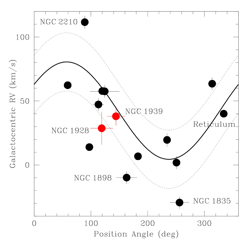
Figure 8: Galactocentric RVs versus PAs diagram for LMC GCs. RVs were taken from the literature (see Table 3). We included the curves derived by van der Marel & Kallivayalil (2014) from $HST$ proper motions of 22 LMC fields (see text for details).

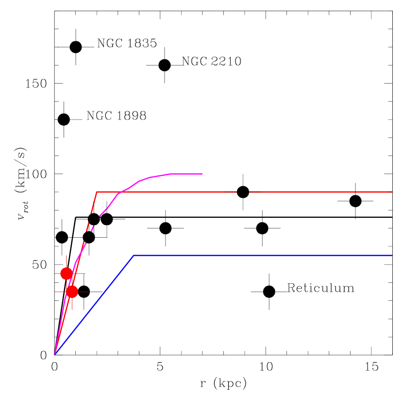
Figure 9: LMC rotation curve as a function of the deprojected distance ($r$) derived from $HST$ proper motions of 22 fields, and from LOS velocities of young and old stellar populations drawn with black, red and blue solid lines, respectively (taken from figure 7 of van der Marel & Kallivayalil, 2014). The rotation curve derived by Vasiliev (2018) is drawn with a magenta line. All the 15 GCs have been superimposed with filled circles; NGC 1928 and 1939 in red.

Table 2: Cluster membership of the observed stars.

ID	Distance to	CMD	RV	[Fe/H]	Adopted
	cluster’s centre
NGC 1928-1	m	m	m	m	m
NGC 1928-2	m	–	m	–	m
NGC 1928-3	m	m	m	m	m
NGC 1928-4	m	–	m	–	m
NGC 1928-5	m	–	nm	–	nm
NGC 1928-6	m	m	m	m	m
NGC 1928-7	m	–	m	–	m
NGC 1928-8	nm	–	nm	nm	nm
NGC 1928-9	nm	–	nm	nm	nm
NGC 1928-10	m	m?	nm	nm	nm
NGC 1928-11	m	m	m	m	m
NGC 1939-1	m	m	nm	m	nm
NGC 1939-2	m	m	nm	nm	nm
NGC 1939-3	m	m	m	m	m
NGC 1939-4	m	m	m	m	m
NGC 1939-5	m	m	m	m	m
NGC 1939-6	m	nm	m	nm	nm
NGC 1939-7	m	m	m	m	m
NGC 1939-8	m	nm	nm	nm	nm
NGC 1939-9	m	m	m	m	m
NGC 1939-10	m	m	m	m	m
NGC 1939-11	m	nm	nm	nm	nm
NGC 1939-12	m	nm	nm	nm	nm
NGC 1939-13	m	m	m	m	m
NGC 1939-14	m	m	m	m	m
NGC 1939-15	m	m	m	m	m

Table 3: Astrophysical properties of LMC GCs.

ID	PA	$r$	RV	Ref.	[Fe/H]	Ref.	PALOS	$v_{rot.}$
	(deg)	(kpc)	(km/s)		(dex)		(deg)	(km/s)
NGC 1466	250.8$\pm$2.0	8.9$\pm$0.9	200.0$\pm$5.0	1	-1.90$\pm$0.10	10	190.0$\pm$10.0	90.0$\pm$10.0
NGC 1754	234.2$\pm$6.7	2.4$\pm$0.9	234.1$\pm$5.4	3	-1.50$\pm$0.10	5,6	100.0$\pm$10.0	75.0$\pm$10.0
NGC 1786	313.7$\pm$7.7	1.8$\pm$0.9	279.9$\pm$4.9	3	-1.75$\pm$0.10	5,6,7	350.0$\pm$10.0	75.0$\pm$10.0
NGC 1835	256.2$\pm$16.8	1.0$\pm$0.9	188.0$\pm$5.0	3	-1.72$\pm$0.10	5,6	130.0$\pm$10.0	170.0$\pm$10.0
NGC 1841	183.0$\pm$2.0	14.2$\pm$0.8	210.3$\pm$0.9	2	-2.02$\pm$0.10	5	130.0$\pm$10.0	85.0$\pm$10.0
NGC 1898	163.0$\pm$18.5	0.4$\pm$0.9	210.0$\pm$5.0	1	-1.32$\pm$0.10	5,6,8	110.0$\pm$10.0	130.0$\pm$10.0
NGC 1916	124.4$\pm$26.0	0.3$\pm$0.9	278.0$\pm$5.0	1	-1.54$\pm$0.10	9	160.0$\pm$10.0	65.0$\pm$10.0
NGC 2005	113.3$\pm$10.0	1.4$\pm$0.9	270.0$\pm$5.0	1	-1.74$\pm$0.10	5,6,8	280.0$\pm$10.0	35.0$\pm$10.0
NGC 2019	120.1$\pm$8.5	1.6$\pm$0.9	280.6$\pm$2.3	2	-1.56$\pm$0.10	5,6,8	150.0$\pm$10.0	65.0$\pm$10.0
NGC 2210	89.2$\pm$3.0	5.2$\pm$0.9	343.0$\pm$5.0	1	-1.55$\pm$0.10	7,9	140.0$\pm$10.0	160.0$\pm$10.0
NGC 2257	59.1$\pm$1.5	9.8$\pm$0.9	301.6$\pm$0.8	2	-1.77$\pm$0.10	5,7,9	100.0$\pm$10.0	70.0$\pm$10.0
Hodge 11	97.3$\pm$2.8	5.2$\pm$0.9	245.1$\pm$1.0	2	-2.00$\pm$0.10	11	335.0$\pm$10.0	70.0$\pm$10.0
Reticulum	334.1$\pm$2.0	10.2$\pm$0.9	247.5$\pm$1.5	2	-1.57$\pm$0.10	2	170.0$\pm$10.0	35.0$\pm$10.0
NGC 1928	119.0$\pm$20.0	0.6$\pm$0.9	249.6$\pm$12.8	4	-1.30$\pm$0.15	4	85.0$\pm$10.0	45.0$\pm$10.0
NGC 1939	144.2$\pm$16.0	0.8$\pm$0.9	258.8$\pm$7.4	4	-2.00$\pm$0.15	4	130.0$\pm$10.0	35.0$\pm$10.0

Ref.: (1)Schommer et al. (1992); (2)Grocholski et al. (2006); (3)Sharma et al. (2010); (4) this work; (5)Suntzeff et al. (1992); (6)Beasley et al. (2002); (7)Mucciarelli et al. (2010); (8)Johnson et al. (2006); (9)Wagner-Kaiser et al. (2018); (10)Walker (1992); (11)Mateluna et al. (2012).

6 Conclusions

With the aim of investigating the origin of the LMC GCs NGC 1928 and 1939, we carried out spectroscopic observations of giant stars located in their fields with the GMOS and the AAOmega+2dF spectrographs of the Gemini South and the Australian Astronomical Observatories, respectivey. The targets were selected bearing in mind their positions along the red giant branch or red clump in $HST$ cluster CMDs, the only available photometric data set at the moment of preparing the observations. Some few candidates without $HST$ photometry were also selected.

The resulting high S/N spectra centred on the Ca II infrared triplet allowed us to measure accurate individual RVs for 11 and 15 stars in the fields of NGC 1928 and 1939, respectively. The RVs were obtained through cross-correlation of the observed spectra with template spectra. We also measured equivalent widths of the three Ca II lines and derived individual metallicities ([Fe/H]) for those stars with available photometry using a previous well-established calibration. The accuracy in the individual [Fe/H] values ranges 0.1-0.3 dex.

By considering as membership probability criteria the position of the observed stars in the cluster CMDs, and their position in the RV and metallicity distribution functions, we concluded that 7 and 9 observed stars are probable cluster members of NGC 1928 and 1939, respectively. The combined three criteria resulted to be a robust approach to assess the cluster membership of the observed stars. From the adopted cluster members we estimated for the first time accurate mean cluster RVs and metallicities. We found that NGC 1928 is one of the most-metal rich GCs ([Fe/H]=-1.3 dex), and NGC 1939 is one of the most metal-poor ones ([Fe/H]=-2.0 dex).

Both GCs are located in the innermost region of the LMC (deprojected distance < 1 kpc) and have RVs consistent with being part of the LMC disc. Therefore, we rule out any possible origin but that in the same galaxy. Indeed, we computed the best solution for a rotation disc that fully contains each GC, separately, and found that the resulting circular velocities at the deprojected cluster distances very well match the rotation curves fitted from $HST$ and $Gaia$ DR2 proper motions, respectively.

We extended our kinematics analysis to all the 15 LMC GCs by obtaining also circular velocities. The outcomes show that most of the GCs share the LMC rotation curve. Since they span the whole LMC GC metallicity range with no evidence of a metallicity gradient, we concluded that the LMC disc has existed since the early epoch of the galaxy formation and has also experienced the abrupt chemical enrichment seen in its GC populations in an interval of time of $\sim$ 3 Gyr. Four objects out of the fifteen GCs (NGC 1835, 1898, 2210 and Reticulum) have estimated circular velocities which notably depart from the LMC rotation curve. We think that they are witnesses of having been stripped by the LMC from the SMC, an scenario predicted from numerical simulations of the galaxy dynamical interactions and confirmed from observation of field star populations.

References

- Angelo et al. (2017) Angelo M. S., Santos Jr. J. F. C., Corradi W. J. B., Maia F. F. S., Piatti A. E., 2017, RAA, 17, 4
- Beasley et al. (2002) Beasley M. A., Hoyle F., Sharples R. M., 2002, MNRAS, 336, 168
- Bressan et al. (2012) Bressan A., Marigo P., Girardi L., Salasnich B., Dal Cero C., Rubele S., Nanni A., 2012, MNRAS, 427, 127
- Brocato et al. (1996) Brocato E., Castellani V., Ferraro F. R., Piersimoni A. M., Testa V., 1996, MNRAS, 282, 614
- Carpintero et al. (2013) Carpintero D. D., Gómez F. A., Piatti A. E., 2013, MNRAS, 435, L63
- Carrera et al. (2008) Carrera R., Gallart C., Hardy E., Aparicio A., Zinn R., 2008, AJ, 135, 836
- Ciddor (1996) Ciddor P., 1996, Appl. Opt., 35, 1566
- Cole et al. (2004) Cole A. A., Smecker-Hane T. A., Tolstoy E., Bosler T. L., Gallagher J. S., 2004, MNRAS, 347, 367
- Cole et al. (2005) Cole A. A., Tolstoy E., Gallagher III J. S., Smecker-Hane T. A., 2005, AJ, 129, 1465
- Da Costa (2016) Da Costa G. S., 2016, MNRAS, 455, 199
- Dutra et al. (1999) Dutra C. M., Bica E., Claria J. J., Piatti A. E., 1999, MNRAS, 305, 373
- Feitzinger & Weiss (1979) Feitzinger J. V., Weiss G., 1979, A&AS, 37, 575
- Grocholski et al. (2006) Grocholski A. J., Cole A. A., Sarajedini A., Geisler D., Smith V. V., 2006, AJ, 132, 1630
- Husser et al. (2013) Husser T.-O., Wende-von Berg S., Dreizler S., Homeier D., Reiners A., Barman T., Hauschildt P. H., 2013, A&A, 553, A6
- Johnson et al. (2006) Johnson J. A., Ivans I. I., Stetson P. B., 2006, ApJ, 640, 801
- Leaman et al. (2013) Leaman R., VandenBerg D. A., Mendel J. T., 2013, MNRAS, 436, 122
- Mackey & Gilmore (2004) Mackey A. D., Gilmore G. F., 2004, MNRAS, 352, 153
- Mateluna et al. (2012) Mateluna R., Geisler D., Villanova S., Carraro G., Grocholski A., Sarajedini A., Cole A., Smith V., 2012, A&A, 548, A82
- Mucciarelli et al. (2010) Mucciarelli A., Origlia L., Ferraro F. R., 2010, ApJ, 717, 277
- Olsen et al. (2004) Olsen K. A. G., Miller B. W., Suntzeff N. B., Schommer R. A., Bright J., 2004, AJ, 127, 2674
- Olsen et al. (2011) Olsen K. A. G., Zaritsky D., Blum R. D., Boyer M. L., Gordon K. D., 2011, ApJ, 737, 29
- Piatti (2017) Piatti A. E., 2017, A&A, 606, A21
- Piatti & Geisler (2013) Piatti A. E., Geisler D., 2013, AJ, 145, 17
- Piatti & Mackey (2018) Piatti A. E., Mackey A. D., 2018, MNRAS, 478, 2164
- Piatti et al. (2009) Piatti A. E., Geisler D., Sarajedini A., Gallart C., 2009, A&A, 501, 585
- Pryor & Meylan (1993) Pryor C., Meylan G., 1993, in Djorgovski S. G., Meylan G., eds, Astronomical Society of the Pacific Conference Series Vol. 50, Structure and Dynamics of Globular Clusters. p. 357
- Rutledge et al. (1997) Rutledge G. A., Hesser J. E., Stetson P. B., Mateo M., Simard L., Bolte M., Friel E. D., Copin Y., 1997, PASP, 109, 883
- Schommer et al. (1992) Schommer R. A., Suntzeff N. B., Olszewski E. W., Harris H. C., 1992, AJ, 103, 447
- Sharma et al. (2010) Sharma S., Borissova J., Kurtev R., Ivanov V. D., Geisler D., 2010, AJ, 139, 878
- Starkenburg et al. (2010) Starkenburg E., et al., 2010, A&A, 513, A34
- Suntzeff et al. (1992) Suntzeff N. B., Schommer R. A., Olszewski E. W., Walker A. R., 1992, AJ, 104, 1743
- Tonry & Davis (1979) Tonry J., Davis M., 1979, AJ, 84, 1511
- Van der Swaelmen et al. (2013) Van der Swaelmen M., Hill V., Primas F., Cole A. A., 2013, A&A, 560, A44
- Vasiliev (2018) Vasiliev E., 2018, preprint, (arXiv:1805.08157)
- Wagner-Kaiser et al. (2017) Wagner-Kaiser R., et al., 2017, MNRAS, 471, 3347
- Wagner-Kaiser et al. (2018) Wagner-Kaiser R., Mackey D., Sarajedini A., Cohen R. E., Geisler D., Yang S.-C., Grocholski A. J., Cummings J. D., 2018, MNRAS, 474, 4358
- Walker (1992) Walker A. R., 1992, AJ, 104, 1395
- Walker et al. (2006) Walker M. G., Mateo M., Olszewski E. W., Bernstein R., Wang X., Woodroofe M., 2006, AJ, 131, 2114
- van den Bergh (2004) van den Bergh S., 2004, AJ, 127, 897
- van der Marel & Kallivayalil (2014) van der Marel R. P., Kallivayalil N., 2014, ApJ, 781, 121
- van der Marel et al. (2002) van der Marel R. P., Alves D. R., Hardy E., Suntzeff N. B., 2002, AJ, 124, 2639