Iterated Greedy Algorithms for the Hop-Constrained Steiner Tree Problem

Abstract

The Hop-Constrained Steiner Tree problem (HCST) is challenging NP-hard problem arising in the design of centralized telecommunication networks where the reliability constraints matter. In this paper three iterative greedy algorithms are described to find efficient optimized solution to solve HCST on both sparse and dense graphs. In the third algorithm, we adopt the idea of Kruskal algorithm for the HCST problem to reach a better solution. This is the first time such algorithm is utilized in a problem with hop-constrained condition. Computational results on a number of problem instances are derived from well-known benchmark instances of Steiner problem in graphs. We compare three algorithms with a previously known method (Voss’s algorithm 14 ) in term of effectiveness, and show that the cost of the third proposed method has been noticeably improved significantly, 34.60$\%$ in hop 10 on dense graphs and 3.34$\%$ in hop 3 on sparse graphs.

1 Introduction

Consider an undirected graph G=(V, E) with $v=\{1,2,...,n\}$, where specific vertex 1 is root vertex and edge set is $E=\{(i,j):i,j\in V,i<j\}$, that each edge has an associated cost $c_{ij}\geq 0$. Also, we define a positive integer $H$ to show the maximum allowance distance of edge from the root. Let $T$ be a tree in $G$, and let $V(T)$ be the set of vertices belonging to $T$. Our goal is finding a tree $T$, rooted at vertex 1, subject to constraints and the number of edges $h_{i}$ between $i\in V(T)$ and the root vertex limited to the maximum value H.

Since HCST is a generalization of Steiner tree problem, it is Np-hard problem109 . We consider hop constraints in graph because of reasons such as reliability or transmission delay in networks. The extensive uses of hop constraints in various settings have been proposed in the literature 103 ; 102 ; 101 ; 107 ; 108 . Intensive researches on the Minimum Spanning Tree problem with hop constraints (HCMST), which is a special case of the HCST problem where all vertices in the graph are terminals exist. Many surveys regarding of HCMST problem can be found in 5 ; 111 ; 110 . Though, there aren’t much attention to Steiner tree problem with hop constraints. In 7 , Gouveia has mentioned HCST problem with developing a strengthened version of a multi-commodity flow model for the minimum spanning tree problem. The LP lower bounds of this model are equal to the ones from a Lagrangian relaxation approach of a weaker MIP model introduced by Gouveia in 8 . Voss presents MIP formulations based on Miller-Tucker-Zemlin subtour elimination constraints 14 . The formulation is then strengthened by disaggregation of variables indicating used edges. The author develops a simple heuristic to find starting solutions and improves them with an exchange procedure based on tabu search. Gouveia Also gives a survey of hop-indexed tree and flow formulations for the hop constrained spanning and Steiner tree problem in 9 . Costa et. al. give a comparison of three methods for a generalization of the HCSTP which is called Steiner tree problem with revenues, budget and hop constraints (STPRBH) in 1 . The considered methods comprise greedy algorithm, destroy-and-repair method and tabu search approaches. Computational results are reported for instances with up to 500 vertices and 12500 edges. Costa et al. in 2 introduce two new models for he STPRBH. Both models are based on the generalized sub-tour elimination constraints and a set of exponential size hop constraints. The authors provide a theoretical and computational comparison with two models based on Miller-Tucker-Zemlin constraints presented in Gouveia 10 and Voss 14 . Theoretical and computational comparisons of flow-based vs. path-based mixed integer programming models for HCST problem are presented by Gouveia et al.. They propose formulations to solve the problem with promising optimality and implement branch-and-price algorithms for all of the formulations11 . Boeck et al. used layered graphs for hop constrained problems to build extended formulations by techniques presented to reduce the size of the layered graphs65 . They also presented variation of this problem arising in the context of multicast transmission in telecommunications. Dokeroglu et al. recently proposed novel self-adaptive and stagnation-aware breakout local search algorithm for the solution of Steiner tree problem with revenue, budget and hop constraints with parallel algorithms 15 . In this paper, we focus on efficient optimization iterative greedy algorithms to find efficient solution for HCST. The new algorithms find a feasible solution for HCST are based on Voss’s approach in 14 . The main feature of our last proposed algorithm is that it uses the idea of Kruskal algorithm in the problem with hop constraint for the first time and enhances the results of this NP-hard problem in polynomial time.

The rest of this paper is organized as following. In Section 2 we formulate a model for HCST problem. Section 3 and 4 provide two complement greedy algorithms to solve HCST. In Section 5 we propose Non Root Based Insertion Algorithm based on the idea of Kruskal algorithm3 . In Section 6 we report extensive set of computational experiments with our iterative greedy algorithms on well known benchmark, consisting variant kinds of graphs. Finally, Section 7 presents concluding remarks .

2 Mathematical formulation

A non-directed graph $G=(V,E)$ is given with edge cost $c_{ij}\geq 0$, $(i,j)\in E$. Let consider the set $Q\subseteq V$ represent basic vertices. To obtain a subgraph with minimum cost, other vertices could be involved. Such vertices are called Steiner vertices $(S=V-Q)$. Consider $x^{p}_{ij}$ as an edge $(i,j)\in E$ that shows the $p^{th}$ position from the root and $\delta(S)$ as a set of edges with one vertex from $S$. The HCST model can be written as follow:

$$min\sum_{p=1}^{H}\sum_{(i,j)\in E}c_{ij}x_{ij}^{p}$$ (1)

$$\sum_{p=1}^{H}\sum_{(i,j)\in\delta(S)}x_{ij}^{p}\geq 1\hskip 28.45274pt\forall S\subseteq V,S\cap Q\neq\emptyset,(V\backslash S)\cap Q\neq\emptyset$$ (2)

$$x_{ij}^{p}\in\{0,1\}\hskip 28.45274pt\forall(i,j)\in E$$ (3)

The goal is to find a subgraph with minimum cost due to the hop constraints; Constraints in (2) present the connectivity constraints of basic vertices attaching to at least one edge of the vertices from $S$ and index $p$ is used to avoid creation of any cycle.

3 Minimum-Hop Iterative Greedy (MinHIG) Algorithm

In this section, we present an iterative greedy algorithm for HCST problem. The basic idea is from 14 . The first three steps of the algorithm use the generalization of prime algorithm 12 considering the path with number of hop instead of a direct edge between two vertices (Algorithm 1).

We start with a partial solution $G=({root},\emptyset)$ that just contains the root. As we mentioned before, $Q$ is the set of all basic vertices. At each step the set $T$ is equal to $Q\backslash G$ and $H$ is the maximum allowed number of hops that the root can connects other vertices in the tree. Suppose $V_{G}$ denote the vertex set of $G$ and $V_{T}$ denote the vertex set of $T$. Cost of path $p(u,v)$ between vertices $u$ and $v$ is presented by $d_{uv}$. Also, for every vertex $v$, we define $U_{v}$ equal to the number of needed hops to reach $v$ from the root. For initialization, we set $U_{root}$ to zero. Phase 1 in MinHIG algorithm finds $U_{v}$ for all vertices $v$.

input : An undirected graph.

output : Find U values.

Step 1. Initialization $G=(\{root\},\emptyset)$;

while $Q\not\subseteq G$ do

       Step 2. Find vertices $u^{*}\in V_{G}$, $v^{*}\in V_{T}$ and path $P(u^{*},v^{*})$, where

      $U_{v}^{*}=U_{u}^{*}+|P(u^{*},v^{*})|\leq H$,

      $d_{u^{*}v^{*}}=min⁡\{d_{uv}|u\leq V_{G},v^{*}\in V_{T}\}$;

      Step 3. Add the vertices and edges of path $P(u^{*},v^{*})$ to G,

      update U values of the vertices of path $P(u^{*},v^{*})$.

Algorithm 1 MinHIG algorithm (Phase 1)

input : U values.

output : An efficient feasible solution.

Step 1. Initialization $Tree=(\{root\},\emptyset)$, h=1;

while $h\neq H$ do

      

      Step 2. Find vertices $u^{*}\in Q$, $v^{*}\in V_{Tree}$, and path $P(u^{*},v^{*})$, where

      $U_{u}^{*}=h$,

      $d_{u^{*}v^{*}}=min⁡\{d_{u^{*}v}|v\in V_{Tree},U_{u^{*}v^{*}}=U_{u}^{*}+|P(u^{*},v^{*})|\leq H\}$;

      Step 3. Add the vertices and edges of path $P(u^{*},v^{*})$ to Tree.

      $h\leftarrow h+1$

Algorithm 2 MinHIG algorithm (Phase 2)

Note that in MinHIG algorithm, we suppose that in the efficient optimal solution, vertices with high $U$ values are connected to vertices with low $U$ values.

In phase 2 in MinHIG, first we add the root vertex to the final tree $Tree$. Then, we start with $h=1$ and and add it until reach maximum hop constraint $h=H$. Vertices with fewer number of hops have been added to the tree earlier. Therefor, with constraint $U_{u}^{*}+|P(u^{*},v^{*})|\leq H$, we find $P(u^{*},v^{*})$, which is the shortest path among all paths of vertex $u^{*}$ to the all previous added vertices to $Tree$. Thus, all edges and vertices of this path will be added to the $Tree$. We repeat this procedure until $Tree$ contains all basic vertices. Figure 1 shows an example of instances where MinHIG gets a solution while Voss’s algorithm 14 doesn’t work.

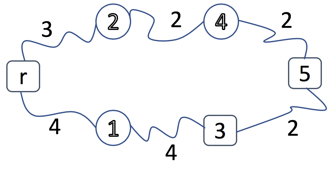
Figure 1: An illustrative example to build HCST with 3 mandatory vertices and 3 Steiner vertices(Circles).

For Figure 1 consider maximum allowed $H$ is 3. With Voss’s algorithm 14 , at first, path $P(r\rightarrow 2\rightarrow 4\rightarrow 5)$ with cost 7 is added to the tree. Then path $P(r\rightarrow 1\rightarrow 3)$ with cost 8 will be added. The final Steiner tree is built has cost 15, although, it is obvious that the optimal cost of the Steiner tree is 10. In Step 3 in phase 2 of Algorithm 1 we have tree reconstruction which gives us the cost of 10 for this example. Suppose that vertices with higher amount of $U$ should be connected to the vertices with lower $U$ values. Therefore, in Step 3 in phase 2, without considering set G, vertices with less U values are added to the final tree. In fact, when we add each vertex, we are sure that other vertices with lower $U$ have been added to the tree earlier and if the current vertex should be connected to one of the basic vertices, we are sure that all possible vertices have been already added to the tree. With implementation of MinHIG on this specific example, after first phase values of $U_{r}=0,U_{1}=1,U_{3}=2,U_{2}=1,U_{4}=2,$ and $U_{5}=3$ have been obtained. After the root is added, basic vertex 3 with the lowest $U$ value among basic vertices with shortest path $P(r\rightarrow 1\rightarrow 3)$ and cost 8 will be added to the tree. Then, the next basic vertex which has not been added to the $Tree$ yet and has minimum value $U$ is vertex 5 with shortest path $P(3\rightarrow 5)$ and cost 2. At the end, the cost of $Tree$ would be 10.

4 Maximum Hop Iterative Greedy (MaxHIG) Algorithm

In MinHIG algorithm, it was assumed that in the Steiner tree, the vertices with higher $U$ are connected to vertices with lower $U$ ,but this approach doesn’t cover all groups of graphs. There are other kinds of graphs in which the vertices by lower hops are connected to the path of the other vertices with more hops. For example, consider Figure 2 where maximum allowed number of $H$ is 4.

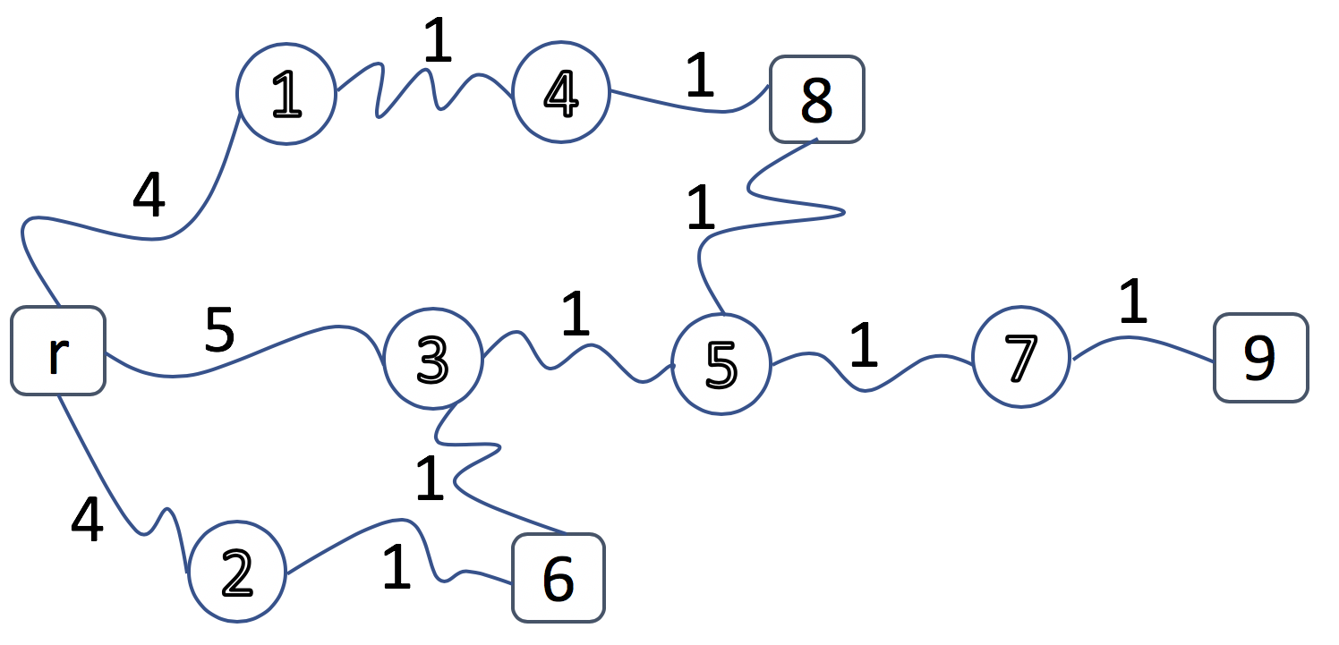
Figure 2: An illustrative example to build HCST with 4 mandatory vertices and 6 Steiner vertices

By MinHIG algorithm, first we add path $P(r\rightarrow 2\rightarrow 6)$ with cost 5 to the $Tree$. Then, path $P(r\rightarrow 1\rightarrow 4\rightarrow 8)$ with cost 6 and path $P(r\rightarrow 3\rightarrow 5\rightarrow 7\rightarrow 9)$ with cost 8 will be added to the $Tree$ respectively. Therefor, the result cost of the achieved Steiner tree by this algorithm would be 19, while the optimal cost is 10.

input : An undirected graph.

output : An efficient feasible solution.

Run Algorithm 1

Step 1. Initialization $Tree=(\{root\},\emptyset)$, h=H;

while $h\neq 1$ do

      

      Step 2. Find vertices $u^{*}\in Q$, $v^{*}\in V_{Tree}$, and path $P(u^{*},v^{*})$, where

      $U_{u}^{*}=h$,

      $d_{u^{*}v^{*}}=min⁡\{d_{u^{*}v}|v\in V_{Tree},U_{u^{*}v^{*}}=U_{u}^{*}+|P(u^{*},v^{*})|\leq H\}$.

      Step 3. Add the vertices and edges of path $P(u^{*},v^{*})$ to Tree.

Algorithm 3 MaxHIG algorithm

For these types of graphs we substitute algorithm MinHIG phase 2 (Algorithm 2) with MaxHIG algorithm (Algorithm3). The following is implementation of algorithm MaxHIG on the example of Figure 2:

First we start with vertex 9 which has the maximum $U$, $U_{9}=4$, and add path $P(3\rightarrow 5\rightarrow 7\rightarrow 9)$ with cost 8 to the tree $Tree$. In the next step, vertex 8 with $U_{8}=3$ and cost 1 will be added to the tree. Then, the path $P(3\rightarrow 6)$ with cost 1 is added to the tree. The final result cost of the $Tree$ would be 10.

In fact, these two greedy algorithms are helpful for two different types of trees with different features. The first category that is solved with MinHIG are graphs, which in their optimal Steiner tree the basic vertices with high amount hops, $U$, are connected to the basic vertices with lower $U$. The latter that can be solved with MaxHIG are graphs that in their optimal Steiner tree, some of the basic vertices are connected to the path of other basic vertices. To obtain Steiner tree in a given arbitrary graph, we run both algorithms and the best answer is considered as the final answer (we will see in last section that in most cases the result by combining of these two algorithms is better than the algorithm by Voss in 14 ). The complexity analysis of presented algorithms is as follows:
-$O(QEH)$ is needed to find the shortest path between basic vertices.
-$O(ELogE)$ is need for Prim algorithm implementation.
-$O(QV)$ is need for adding a basic vertex at each time and the comparison to all vertices inside $Tree$.

5 Non Root Based Insertion (NRBI) Algorithm

In this part, first we give an informal overview of NRBI algorithm and then we present the analysis in details. The algorithm uses generalized idea of both Prime and Kruskal algorithm. We use new variable $itr_{v}$ (Algorithm 4) to every basic vertex $v$ as time of entrance to the set $G$. Again here We assume that $itr_{root}$ is zero at first and then the first basic vertex $v$ entered to set $G$ after root has $itr_{v}=1$. In phase 2 of NRBI algorithm, basic vertices are sorted in descending order due to their $iter$ amount. Then, they would be added to the $Tree$ similar to idea of Kruskal algorithm. In the Voss’s algorithm, the final tree is a subset of set $G$ constructed in the first phase. In MinHIG and MaxHIG algorithms, set $G$ is completely neglected and the final tree is created only based on $U$ values. In this algorithm, as we will see further, set $G$ is used as an auxiliary set. When vertex $v$ is added to the tree, there will be two cases:

1- Connecting vertex $v$ to vertices with less $itr$.

2- Connecting vertex $v$ to vertices, which will be added to $G$ after vertex $v$.

In the former one, the result is clear and vertex $v$ should be connected to same vertices that it was connected to in $G$. If the latter, result will not be clear. First we have to find all vertices with more $itr$ than $v$ to find the needed Steiner vertices and add them to the $Tree$ and then we add vertex $v$. Suppose all vertices except basic vertex $v$ have been added in the optimal tree and now we have to add the last remaining vertex $v$ to the Steiner tree. For similar conditions without loss of generality, we assume that the tree is two pieces. First one contains all vertices with $itr$ less than $k$ (this sub-tree may be a sub-forest and consists of many disconnected sub-trees) and second one is optimal sub-tree containing all vertices with $itr$ value more than $k$. Our goal is to connect $v$ to the first or second set in the best way. Each time, vertex $v$ is connected to one of the two pieces until we get the whole tree of all vertices especially vertex $v$. The optimal sub-tree of the first set of the vertices with $itr$ less than $k$ is the optimal sub-tree generated by the set $S$ containing all vertices added before $v$ to $S$.

input : An undirected graph.

output : U and itr values.

Step 1. Initialization $G=(\{root\},\emptyset)$,

while $Q\not\subseteq S$ do

      

      Step 2. Find vertices $u^{*}\in V_{G}$ and $v^{*}\in V_{T}$ and path P(u*,v*), where

      $U_{v}^{*}=U_{u}^{*}+|P(u^{*},v^{*})|\leq H$,

      $d_{u^{*}v^{*}}=min⁡\{d_{uv}|u\leq V_{G},v^{*}\in V_{T}\}$;

      Step 3. Add the vertices and edges of path $P(u^{*},v^{*})$ to G,

      update U values of the vertices of path $P(u^{*},v^{*})$,

      Save $itr[BasicVertex\hskip 5.69046ptv\in P(u^{*},v^{*})]$.

Algorithm 4 NRBI (Phase 1)

input : $U_{i}$ and itr.

output : An efficient feasible solution.

Initialization $Tree=\{\emptyset\}$

for Maximum $Itr_{v}$ to 1 do

      

      Find $P(v,u^{*})$ where

      $u^{*}\in Tree$,

      $U_{u}^{*}+|P(u^{*},v)|\leq U_{v}$;

      if $Cost(P(v,u^{*}))<Cost(P(v,u^{*})\in G)$ then

            

      Add all vertices and edges of $P(v,u^{*})$ to Tree.

      else

             Add all vertices and edges of $P(v,u^{*})\in G$ to Tree.

      

Algorithm 5 NRBI (Phase 2)

Now we want to find the most optimal connection of the vertex $v$ to the tree. So, in the second step, we try to make the best connections for optimal subtree of $v$. Since having $U$ values generated from the first phase of the generalized of prim algorithm, we can guarantee that the hop constraint is not violated. In the second part of the algorithm, by inspiring the idea of Kruskal algorithm, we allow to connect each vertex to other vertices without violating $U$ (Algorithm 5).

The analysis of NRBI algorithm

Here we analyze our algorithm in details. We show that the output is tree and the constructed set doesn’t include any cycle or cross. All basic vertices in $Q$ are connected together with $Q-1$ paths by idea of Kruskal algorithm. Because all $U$ values generated in the phase 1 are connected by this precondition that each vertex can only be connected to the vertex with less $U$, so no cycle would be created.

Since, in this problem we consider adding path instead of edge due to of the idea of Kruskal algorithm, we should show that no cross is gonna happened either. In NRBI algorithm, we connect vertices based on their $itr$ in descending order. The cross happens when some vertices of some paths are connected to each other. Since we know that paths that are constructed by vertices with more $itr$. These vertices are the only ones capable of changing $U$ values of vertices that are produced before in path by lower $itr$ and reverse of it is not possible. Thus cross wont happen. In the second phase of the algorithm, when we add vertices with more $itr$ to the forest respectively, we assure that during choosing a shortest path for each basic vertex, no cross will be created (No changes can happen in previous paths of the forest). To find the closest vertex to the current $itr$, distances from all basic and Steiner vertices that have been added to the $Tree$ before are calculated. Thus, there wont be any possibility of creating the cross. If we assume that cross is created, so the vertex at the intersection has been added to the $Tree$ before, then the vertex with current $itr$ was closer to the vertex of the cross and this is in contrast to our assumption that we have connected the current vertex to the closest vertex with respect to hop constraint. Therefore, there is no cross in graph and the result is tree.

Time complexity of this algorithm in the first part is similar to the previous presented algorithms, equal to $O(ELogE)$. In the second part in tree construction, all vertices are connected to each other in the forest. Since for every basic vertex when we add it, it will be compared to all the Steiner and basic vertices in the tree, thus the running time is $O(QV)$. Before, in the generalized Bellman-Ford, all paths from vertices to each other were calculated in time $O(QEH)$ and stored in the table. The only cost that we nee to calculate to find the path is the time of adding selected path from the table for every vertex in $Q$ which is at most $H$. Therefor, the time complexity would be $O(QH)$ and the total time of last part of the algorithm is $O(QV$).

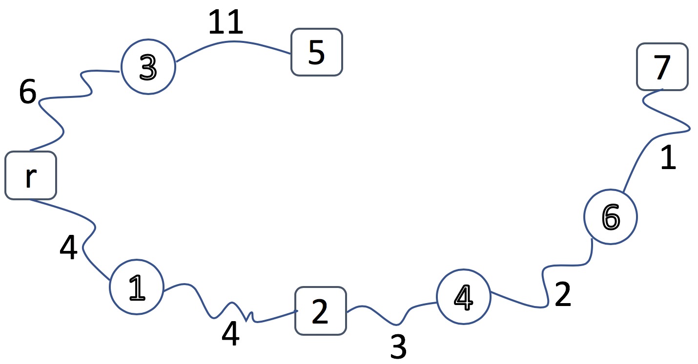
Figure 3: An illustrative example to build HCST with 4 mendatory vertices and 4 Steiner vertices

Figure 3 presents an example that if we apply all previous algorithms on that we obtain 31 as the optimal Steiner tree. Though here is the implementation of the NRBI algorithm on the same graph:

First Step:

First, paths $P(r\rightarrow 1\rightarrow 2)$ with cost 8 and basic vertex 2, $P(2\rightarrow 4\rightarrow 6\rightarrow 7)$ with cost of 6 and basic vertex 7, and then path $P(r\rightarrow 3\rightarrow 5)$ with cost 17 are added to set $G$ respectively. Now we see that set $G$ contains all basic vertices.

The updated variables $itr$ and $U$ are as follows,

$itr_{7}=2,itr_{5}=3,itr_{2}=1,$ and $itr_{0}=0$,

$U_{5}=2,U_{2}=2,U_{7}=5,$ and $U_{0}=0$

Second Step:

So, we added basic vertices 0,2,5,7 to the tree. Starting with the basic vertex with maximum $itr$, we select vertex 5. The shortest path between vertex 5 and existed vertices $u^{*}$ in set $Tree$ with $U_{u}^{*}+|P(u^{*},5)|\leq U_{5}$ is $P(r\rightarrow 3\rightarrow 5)$ . All edges and vertices of this path are added to the tree (This path is the same path of vertex 5 in set $G$).

The next basic vertex is the one with itr = 2, which is vertex 7. The best way to connect vertex 7 to the one of the vertices in the set $Tree$ is path $P(2\rightarrow 4\rightarrow 6\rightarrow 7)$ with cost 6. For next vertex with $itr=1$, vertex 2, the best way to connect it to one of the vertices of the tree is $P(2\rightarrow 3)$ with cost 7. Although the best path for 2 in $G$ is $P(r\rightarrow 1\rightarrow 2)$ with cost 8, we add vertex 2 with cost 7. The optimal Steiner tree with cost 30 is obtained.

Note, the tree at the beginning of the second phase is not connected same as idea of Kruskal algorithm when we add edges to find the shortest path, but with adding $Q-1$ paths, at the end the Steiner tree would be a connected tree.

6 Computation

In order to assess the performance of all proposed algorithms, we used instances $\{c,d\}$n, $n\in\{5,10,15,20\}$ randomly chosen from the OR-Library[6].

The size of these instances for ST problem have been defined between 500 and 1000 nodes from 625 up to 25000 edges (see 105 for more details about these instances).

In general, ST instances generate HCST input graphs in this way that ST files provide edge-costs and Steiner vertices so that we select 200 and 300 basic vertices due to random vectors. All algorithms have been implemented in C++ and run on all instances, sparse graphs $\{c5,c10,d5,d10\}$ and dense graphs $\{c15,c20,d15,d20\}$.

For the sake of quality of all algorithms for every sample library, we generate number of vectors equal to 100 times of the hop limitation $H$ to specify different group of basic vertices. For example, to implement the algorithms on instances for $H=3$, we generate 300 vectors to create different groups of basic vertices.

All algorithms have been implemented on every vector on every instances. Therefore, the number of implementation for every algorithm on specified hop is equal to $100H\times 16$. We compare all of our algorithms with algorithm in 14 (Named in the table Voss). In the tables, MinHIG algorithm, MaxHIG algorithm, and NRBI algorithm are represented as MinH, MaxH, and NRBI respectively. We also combine first two algorithms, MinHIG and MaxHIG, and show the results of this combination as MM in our tables.

Tables 1 to 8 compare results of algorithms as follows:

First algoritm vs second algorithm: FOS,   SFOS,   SOF, and   SSOF

FOS = represents number of times that results of first algorithm is better than the second one.

SFOS = sum of the cost amount that the first algorithm is less than the second one.

SOF= represents the number of times that results of the second algorithm is better than the first one.

SSOF= sum of the cost amount that the second algorithm is less than the first one.

In the following, we show that how we compare results of every two algorithms in every row of the table:

For example: Voss vs MinH: 6   20    224   2739 means that in this comparison the Voss’s algorithm is 6 times better than MinH and the sum of the difference of their cost is 20. MinH is 224 times better than Voss and the sum of the difference of their cost is 2739.

Tests are based on the benchmarks c and d with 200 and 300 basic vertices for 3, 5, 7, and 10 hop. Tables 1 to 4 present our computational results on sparse sets $\{c5,d5\}$ and $\{c10,d10\}$ with 200 and 300 basic vertices, respectively. We focus on NRBI and MM to show that they are the best ones among all five algorithms, but all algorithms are compared two each other one by one and results are provided in tables 1 to 8.

For $H=3$, in 8.54$\%$ of 300 vectors, NRBI is better than Voss algorithm. The cost difference is 69.12 in average. In the rest percent of the vectors, the cost calculation for both Voss and NRBI are the same, and in no cases Voss could get better than NRBI. For this hop limitation, We also saw MM is better than Voss with cost difference 49.37 in 5.79$\%$ of 300 vectors and in 2.5$\%$ vectors, Voss is better with cost difference 21.62 . In the remaining ones, two algorithms found the same cost.

For $H=5$, NRBI in 67.37$\%$ of 500 vectors is better compared to the Voss’s algorithm, with cost difference 12940.11 in average. In the remaining percent of the vectors the cost calculations for both Voss and NRBI are equal, and in no cases Voss was seen better than NRBI. In this hop, we also found that in 52.27$\%$ of 500 vectors, MM is better than Voss with cost difference 5879. In 14.2$\%$ vectors Voss is better with cost difference 638 and in the remaining ones two algorithms found the result with similar cost.

For $H=7$, NRBI in 99.71$\%$ of 700 vectors is better than Voss with cost difference 34029.62 in average and for the rest of the vectors, the minimum costs found by Voss and NRBI are equal. In no cases Voss is better than NRBI. In this hop, in 63.14$\%$ of 700 vectors MM is better than Voss with cost difference 9040.12 and in 34.30$\%$ with cost 3604.37 vector Voss is better. The remaining vectors, two algorithms calculated same cost.

Methods Comparison c5 d5 Number of Hop FOS SFOS SOF SSOF FOS SFOS SOF SSOF Voss vs MinH: 0 0 0 0 0 0 0 0 Voss vs MaxH: 0 0 0 0 0 0 0 0 Voss vs NRBI: 0 0 0 0 0 0 0 0 Voss vs MM: 0 0 0 0 0 0 0 0 MinH vs MaxH: 0 0 0 0 0 0 0 0 H=3 MinH vs NRBI: 0 0 0 0 0 0 0 0 MinH vs MM: 0 0 0 0 0 0 0 0 MaxH vs NRBI: 0 0 0 0 0 0 0 0 MaxH vs MM: 0 0 0 0 0 0 0 0 NRBI vs MM: 0 0 0 0 0 0 0 0 Voss vs MinH: 0 0 96 638 6 20 224 2739 Voss vs MaxH: 0 0 96 638 22 118 219 2655 Voss vs NRBI: 0 0 96 638 0 0 231 2805 Voss vs MM: 0 0 96 638 4 16 224 2741 MinH vs MaxH: 0 0 0 0 33 188 3 6 H=5 MinH vs NRBI: 0 0 0 0 0 0 21 86 MinH vs MM: 0 0 0 0 0 0 3 6 MaxH vs NRBI: 0 0 0 0 0 0 49 268 MaxH vs MM: 0 0 0 0 0 0 33 188 NRBI vs MM: 0 0 0 0 18 80 0 0 Voss vs MinH: 222 1689 448 5801 281 3297 399 5753 Voss vs MaxH: 382 4682 302 3422 441 7373 240 2814 Voss vs NRBI: 0 0 691 14835 0 0 697 19983 Voss vs MM: 201 1379 470 6515 248 2714 428 6258 MinH vs MaxH: 524 6396 155 1024 512 8103 115 1088 H=7 MinH vs NRBI: 24 68 662 10791 11 26 683 17553 MinH vs MM: 0 0 155 1024 0 0 115 1088 MaxH vs NRBI: 9 48 684 16143 0 0 698 24542 MaxH vs MM: 0 0 524 6396 0 0 512 8103 NRBI vs MM: 651 9811 31 112 682 16465 11 26 Voss vs MinH: 296 5671 697 18648 563 13046 422 8136 Voss vs MaxH: 762 27232 231 4129 921 42692 73 1065 Voss vs NRBI: 0 0 1000 49505 0 0 1000 46771 Voss vs MM: 279 4712 715 19223 553 12259 432 8400 MinH vs MaxH: 894 37614 101 1534 902 37768 92 1051 H=10 MinH vs NRBI: 13 75 986 36603 1 6 999 51687 MinH vs MM: 0 0 101 1534 0 0 92 1051 MaxH vs NRBI: 1 7 999 72615 0 0 1000 88398 MaxH vs MM: 0 0 894 37614 0 0 902 37768 NRBI vs MM: 985 35076 14 82 999 50636 1 6

Table 1: Steiner results on c5 and d5 instances with 200 basic vertices

For $H=10$, in 99.75$\%$ of 1000 vectors, NRBI could find a better solution than Voss with cost difference 9683 in average. In the remaining percent of the vectors Voss and NRBI are equal. In 39.95$\%$ of 1000 vectors, MM is better than Voss with cost difference 38545.75. Also, Voss is better in 58.67$\%$ vectors with cost difference 1789.75.Remaining had same results.

Methods Comparison c5 d5 Number of Hop FOS SFOS SOF SSOF FOS SFOS SOF SSOF Voss vs MinH: 0 0 0 0 0 0 0 0 Voss vs MaxH: 0 0 0 0 0 0 0 0 Voss vs NRBI: 0 0 0 0 0 0 0 0 Voss vs MM: 0 0 0 0 0 0 0 0 MinH vs MaxH: 0 0 0 0 0 0 0 0 H=3 MinH vs NRBI: 0 0 0 0 0 0 0 0 MinH vs MM: 0 0 0 0 0 0 0 0 MaxH vs NRBI: 0 0 0 0 0 0 0 0 MaxH vs MM: 0 0 0 0 0 0 0 0 NRBI vs MM: 0 0 0 0 0 0 0 0 Voss vs MinH: 94 518 46 264 7 22 52 459 Voss vs MaxH: 160 670 48 269 64 230 250 2929 Voss vs NRBI: 0 0 116 540 0 0 253 3107 Voss vs MM: 74 365 54 304 1 3 252 2950 MinH vs MaxH: 109 340 39 193 67 248 220 2510 H=5 MinH vs NRBI: 6 36 152 830 0 0 222 2670 MinH vs MM: 0 0 39 193 0 0 220 2510 MaxH vs NRBI: 7 34 217 975 0 0 112 408 MaxH vs MM: 0 0 109 340 0 0 67 248 NRBI vs MM: 130 642 7 41 46 160 0 0 Voss vs MinH: 291 2909 387 5108 171 1623 513 8615 Voss vs MaxH: 358 5280 317 4029 350 5619 340 5118 Voss vs NRBI: 0 0 698 17979 0 0 698 19602 Voss vs MM: 221 1922 453 6487 134 1080 548 9751 MinH vs MaxH: 424 5816 247 2366 515 9172 170 1679 MinH vs NRBI: 5 13 693 15793 19 80 673 12690 H=7 MinH vs MM: 0 0 247 2366 0 0 170 1679 MaxH vs NRBRI: 5 13 693 19243 5 26 693 20129 MaxH vs MM: 0 0 424 5816 0 0 515 9172 NRBI vs MM: 687 13436 9 22 666 11037 24 106 Voss vs MinH: 277 5560 718 25206 380 7035 598 14452 Voss vs MaxH: 711 27168 279 7472 784 31241 207 3655 Voss vs NRBI: 0 0 1000 64750 0 0 1000 62950 Voss vs MM: 270 5223 725 25720 352 6131 628 15403 MinH vs MaxH: 925 40193 71 851 866 36858 126 1855 H=10 MinH vs NRBI: 14 92 984 45196 0 0 999 55533 MinH vs MM: 0 0 71 851 0 0 126 1855 MaxH vs NRBI: 1 1 999 84447 0 0 1000 90536 MaxH vs MM: 0 0 925 40193 0 0 866 36858 NRBI vs MM: 983 44346 15 93 999 53678 0 0

Table 2: Steiner results on c5 and d5 instances with 300 basic vertices

Methods Comparison c10 d10 Number of Hop FOS SFOS SOF SSOF FOS SFOS SOF SSOF Voss vs MinH: 21 70 18 64 0 0 0 0 Voss vs MaxH: 29 109 32 105 0 0 0 0 Voss vs NRBI: 0 0 60 166 0 0 0 0 Voss vs MM: 16 46 37 120 0 0 0 0 MinH vs MaxH: 18 78 24 80 0 0 0 0 H=3 MinH vs NRBI: 0 0 63 172 0 0 0 0 MinH vs MM: 0 0 24 80 0 0 0 0 MaxH vs NRBI: 0 0 57 170 0 0 0 0 MaxH vs MM: 0 0 18 78 0 0 0 0 NRBI vs MM: 39 92 0 0 0 0 0 0 Voss vs MinH: 39 327 456 14096 264 3296 222 2386 Voss vs MaxH: 175 2562 317 6787 233 2722 257 2533 Voss vs NRBI: 0 0 500 28924 0 0 500 12442 Voss vs MM: 28 200 468 14740 196 2019 293 3284 MinH vs MaxH: 416 10315 76 771 215 1454 247 2175 H=5 MinH vs NRBI: 1 3 498 15158 0 0 498 13352 MinH vs MM: 0 0 76 771 0 0 247 2175 MaxH vs NRBI: 0 0 499 24699 1 1 498 12632 MaxH vs MM: 0 0 416 10315 0 0 215 1454 NRBI vs MM: 497 14387 1 3 496 11178 1 1 Voss vs MinH: 375 6439 309 4436 497 17432 195 5241 Voss vs MaxH: 680 34162 19 150 347 9000 344 9944 Voss vs NRBI: 0 0 700 23774 0 0 700 52782 Voss vs MM: 374 6287 310 4450 311 7199 378 11278 MinH vs MaxH: 682 32175 17 166 178 3135 517 16270 H=7 MinH vs NRBI: 1 3 699 25780 0 0 700 64973 MinH vs MM: 0 0 17 166 0 0 517 16270 MaxH vs NRBI: 0 0 700 57786 0 0 700 51838 MaxH vs MM: 0 0 682 32175 0 0 178 3135 NRBI vs MM: 699 25614 1 3 700 48703 0 0 Voss vs MinH: 834 14577 149 1182 986 56132 12 150 Voss vs MaxH: 1000 97700 0 0 999 101492 1 23 Voss vs NRBI: 0 0 982 13866 0 0 1000 39112 Voss vs MM: 834 14577 149 1182 985 54496 13 173 MinH vs MaxH: 999 84305 0 0 903 47146 93 1659 H=10 MinH vs NRBI: 0 0 997 27261 0 0 1000 95094 MinH vs MM: 0 0 0 0 0 0 93 1659 MaxH vs NRBI: 0 0 1000 111566 0 0 1000 140581 MaxH vs MM: 0 0 999 84305 0 0 903 47146 NRBI vs MM: 997 27261 0 0 1000 93435 0 0

Table 3: Steiner results on c10 and d10 instances with 200 basic vertices

Tables 5 to 8 present our computational results on dense sets $\{c15,d15\}$ and $\{c20,d20\}$ with 200 and 300 basic vertices, respectively. When $H=3$, NRBI is better than Voss in 100$\%$ of 300 vectors. The cost difference is 9683 in average. In the remaining part of the vectors Voss and NRBI both have equal result, and in no cases Voss is better than NRBI. In this hop, in 58.83$\%$ of 300 vectors, MM is better than Voss with cost difference 2407.12 and in 37.16$\%$ of them Voss gets better with cost 797. For rest of the vectors they calculate same cost.

Method Comparison c10 d10 Number of Hop FOS SFOS SOF SSOF FOS SFOS SOF SSOF Voss vs MinH: 68 266 51 79 0 0 0 0 Voss vs MaxH: 87 311 91 247 0 0 0 0 Voss vs NRBI: 0 0 145 387 0 0 0 0 Voss vs MM: 44 127 102 275 0 0 0 0 MinH vs MaxH: 59 212 93 335 0 0 0 0 H=3 MinH vs NRBI: 0 0 154 574 0 0 0 0 MinH vs MM: 0 0 93 335 0 0 0 0 MaxH vs NRBI: 0 0 116 451 0 0 0 0 MaxH vs MM: 0 0 59 212 0 0 0 0 NRBI vs MM: 81 239 0 0 0 0 0 0 Voss vs MinH: 20 125 473 20236 278 3889 210 2631 Voss vs MaxH: 181 3499 314 7960 281 3901 207 2101 Voss vs NRBI: 0 0 500 36101 0 0 499 18964 Voss vs MM: 16 101 479 20437 218 2686 272 3302 MinH vs MaxH: 472 15875 24 225 253 2416 218 1874 H=5 MinH vs NRBI: 1 1 497 15991 0 0 500 20222 MinH vs MM: 0 0 24 225 0 0 218 1874 MaxH vs NRBI: 0 0 500 31640 0 0 500 20764 MaxH vs MM: 0 0 472 15875 0 0 253 2416 NRBI vs MM: 497 15766 1 1 500 18348 0 0 Voss vs MinH: 194 2423 491 10725 260 6758 435 15972 Voss vs MaxH: 694 48742 3 69 520 22808 176 4618 Voss vs NRBI: 0 0 700 31022 0 0 700 92260 Voss vs MM: 194 2421 491 10730 238 5833 458 16852 MinH vs MaxH: 698 56982 2 7 591 29209 105 1805 H=7 MinH vs NRBI: 1 5 699 22725 0 0 700 83046 MinH vs MM: 0 0 2 7 0 0 105 1805 MaxH vs NRBI: 0 0 700 79695 0 0 700 110450 MaxH vs MM: 0 0 698 56982 0 0 591 29209 NRBI vs MM: 699 22718 1 5 700 81241 0 0 Voss vs MinH : 560 6496 397 3949 861 40240 137 2817 Voss vs MaxH : 1000 127553 0 0 996 138991 4 119 Voss vs NRBI : 0 0 998 20109 0 0 1000 68787 Voss vs MM : 560 6496 397 3949 861 40024 137 2832 MinH vs MaxH : 1000 125006 0 0 989 101680 10 231 H=10 MinH vs NRBI: 1 3 998 22659 0 0 1000 106210 MinH vs MM : 0 0 0 0 0 0 10 231 MaxH vs NRBI: 0 0 1000 147662 0 0 1000 207659 MaxH vs MM : 0 0 1000 125006 0 0 989 101680 NRBI vs MM : 998 22659 1 3 1000 105979 0 0

Table 4: Steiner results on c10 and d10 instances with 300 basic vertices

Methods Comparison c15 d15 Number of Hop FOS SFOS SOF SSOF FOS SFOS SOF SSOF Voss vs MinH: 67 677 227 4224 39 182 250 2380 Voss vs MaxH: 151 2010 137 1738 93 578 190 1439 Voss vs NRBI: 0 0 300 15814 0 0 299 5292 Voss vs MM: 61 583 231 4389 35 169 254 2451 MinH vs MaxH: 255 4078 42 259 238 1421 20 84 H=3 MinH vs NRBI: 0 0 299 12267 1 1 293 3095 MinH vs MM: 0 0 42 259 0 0 20 84 MaxH vs NRBI: 0 0 300 16086 1 3 298 4434 MaxH vs MM: 0 0 255 4078 0 0 238 1421 NRBI vs MM: 299 12008 0 0 292 3014 2 4 Voss vs MinH: 13 141 486 20420 5 22 495 22888 Voss vs MaxH: 304 5007 187 2488 37 221 459 11779 Voss vs NRBI: 0 0 500 21862 0 0 500 21389 Voss vs MM: 306 5019 185 2434 41 241 455 11297 MinH vs MaxH: 488 22864 8 66 440 11810 56 502 H=5 MinH vs NRBI: 0 0 500 19343 0 0 500 32947 MinH vs MM: 0 0 8 66 0 0 56 502 MaxH vs NRBI: 0 0 500 42141 0 0 500 44255 MaxH vs MM: 0 0 488 22864 0 0 440 11810 NRBI vs MM: 500 19277 0 0 500 32445 0 0 Voss vs MinH: 0 0 700 64212 1 3 699 44764 Voss vs MaxH: 97 649 593 10549 6 20 694 21112 Voss vs NRBI: 0 0 699 12872 0 0 700 11019 Voss vs MM: 97 649 593 10549 6 20 694 21016 MinH vs MaxH: 700 54312 0 0 680 23765 18 96 H=7 MinH vs NRBI: 0 0 700 22772 0 0 700 32111 MinH vs MM: 0 0 0 0 0 0 18 96 MaxH vs NRBI: 0 0 700 77084 0 0 700 55780 MaxH vs MM: 0 0 700 54312 0 0 680 23765 NRBI vs MM: 700 22772 0 0 700 32015 0 0 Voss vs MinH: 0 0 1000 123718 0 0 1000 83140 Voss vs MaxH: 39 171 947 18998 0 0 1000 34330 Voss vs NRBI: 0 0 980 7150 0 0 956 5709 Voss vs MM: 39 171 947 18998 0 0 1000 34322 MinH vs MaxH: 1000 104891 0 0 997 48818 3 8 H=10 MinH vs NRBI: 0 0 1000 25977 0 0 1000 40039 MinH vs MM: 0 0 0 0 0 0 3 8 MaxH vs NRBI: 0 0 1000 130868 0 0 1000 88849 MaxH vs MM: 0 0 1000 104891 0 0 997 48818 NRBI vs MM: 1000 25977 0 0 1000 40031 0 0

Table 5: Steiner results on c15 and d15 instances with 200 basic vertices

For $H=5$, in 92.70$\%$ of 500 vectors NRBI result is better than what Voss got with cost difference 13012.25 in average. In the rest percent of the vectors, the min cost calculated by Voss and NRBI are same. In no cases Voss is better than NRBI. For this hop, also in 77.12$\%$ of 500 vectors MM is better than Voss. The cost difference of them is 4101. In 20.8$\%$ of vectors Voss is better with cost difference 1657.62. For rest of the vectors two algorithms calculate same cost.

Methods Comparison c15 d15 Number of Hop FOS SFOS SOF SSOF FOS SFOS SOF SSOF Voss vs MinH: 29 233 268 7410 116 690 179 1768 Voss vs MaxH: 131 2032 162 3205 168 1560 119 1071 Voss vs NRBI: 0 0 300 22042 0 0 300 7822 Voss vs MM: 27 219 271 7594 112 648 181 1856 MinH vs MaxH: 270 6202 25 198 238 1697 45 130 H=3 MinH vs NRBI: 0 0 300 14865 0 0 300 6744 MinH vs MM: 0 0 25 198 0 0 45 130 MaxH vs NRBI: 0 0 300 20869 0 0 300 8311 MaxH vs MM: 0 0 270 6202 0 0 238 1697 NRBI vs MM: 300 14667 0 0 300 6614 0 0 Voss vs MinH: 9 158 490 34526 2 24 498 34875 Voss vs MaxH: 367 7289 120 1084 63 592 434 12094 Voss vs NRBI: 0 0 500 25233 0 0 500 27998 Voss vs MM: 367 7289 120 1067 64 600 433 11977 MinH vs MaxH: 499 40590 1 17 481 23474 17 125 H=5 MinH vs NRBI: 0 0 500 19028 0 0 500 39500 MinH vs MM: 0 0 1 17 0 0 17 125 MaxH vs NRBI: 0 0 500 59601 0 0 500 62849 MaxH vs MM: 0 0 499 40590 0 0 481 23474 NRBI vs MM: 500 19011 0 0 500 39375 0 0 Voss vs MinH: 0 0 700 78845 0 0 700 59576 Voss vs MaxH: 250 2070 421 4763 17 124 677 19948 Voss vs NRBI: 0 0 700 15325 0 0 700 18595 Voss vs MM: 250 2070 421 4763 17 124 677 19940 MinH vs MaxH: 700 76152 0 0 697 39760 1 8 H=7 MinH vs NRBI: 0 0 700 18018 0 0 700 38419 MinH vs MM: 0 0 0 0 0 0 1 8 MaxH vs NRBI: 0 0 700 94170 0 0 700 78171 MaxH vs MM: 0 0 700 76152 0 0 697 39760 NRBI vs MM: 700 18018 0 0 700 38411 0 0 Voss vs MinH: 0 0 1000 145523 0 0 1000 114865 Voss vs MaxH: 90 472 892 11882 2 4 998 36087 Voss vs NRBI: 0 0 992 8653 0 0 994 9344 Voss vs MM: 90 472 892 11882 2 4 998 36087 MinH vs MaxH: 1000 134113 0 0 1000 78782 0 0 H=10 MinH vs NRBI: 0 0 1000 20063 0 0 1000 45427 MinH vs MM: 0 0 0 0 0 0 0 0 MaxH vs NRBI: 0 0 1000 154176 0 0 1000 124209 MaxH vs MM: 0 0 1000 134113 0 0 1000 78782 NRBI vs MM: 1000 20063 0 0 1000 45427 0 0

Table 6: Steiner results on c15 and d15 instances with 300 basic vertices

Methods Comparison c20 d20 Number of Hop FOS SFOS SOF SSOF FOS SFOS SOF SSOF Voss vs MinH: 166 706 105 412 229 1819 57 288 Voss vs MaxH: 286 3298 9 30 293 4831 6 29 Voss vs NRBI: 0 0 300 3484 0 0 300 6621 Voss vs MM: 164 696 107 425 229 1808 57 293 MinH vs MaxH: 289 2997 9 23 289 3287 8 16 H=3 MinH vs NRBI: 0 0 299 3778 0 0 300 8152 MinH vs MM: 0 0 9 23 0 0 8 16 MaxH vs NRBI: 0 0 300 6752 0 0 300 11423 MaxH vs MM: 0 0 289 2997 0 0 289 3287 NRBI vs MM: 299 3755 0 0 300 8136 0 0 Voss vs MinH: 0 0 500 20868 0 0 500 21531 Voss vs MaxH: 14 26 475 3163 5 17 493 5853 Voss vs NRBI: 0 0 380 987 0 0 493 2560 Voss vs MM: 14 26 475 3163 5 17 493 5852 MinH vs MaxH: 500 17731 0 0 499 15696 1 1 H=5 MinH vs NRBI: 0 0 499 4124 0 0 500 8396 MinH vs MM: 0 0 0 0 0 0 1 1 MaxH vs NRBI: 0 0 500 21855 0 0 500 24091 MaxH vs MM: 0 0 500 17731 0 0 499 15696 NRBI vs MM: 499 4124 0 0 500 8395 0 0 Voss vs MinH: 0 0 700 34709 0 0 700 39599 Voss vs MaxH: 0 0 694 5152 1 2 699 8067 Voss vs NRBI: 0 0 231 275 0 0 596 1834 Voss vs MM: 0 0 694 5152 1 2 699 8067 MinH vs MaxH: 700 29557 0 0 700 31534 0 0 H=7 MinH vs NRBI: 0 0 696 5427 0 0 700 9899 MinH vs MM: 0 0 0 0 0 0 0 0 MaxH vs NRBI: 0 0 700 34984 0 0 700 41433 MaxH vs MM: 0 0 700 29557 0 0 700 31534 NRBI vs MM: 696 5427 0 0 700 9899 0 0 Voss vs MinH: 0 0 1000 49957 0 0 1000 64645 Voss vs MaxH: 1 1 990 7125 0 0 1000 13254 Voss vs NRBI: 0 0 263 307 0 0 325 465 Voss vs MM: 1 1 990 7125 0 0 1000 13254 MinH vs MaxH: 1000 42833 0 0 1000 51391 0 0 H=10 MinH vs NRBI: 0 0 994 7431 0 0 1000 13719 MinH vs MM: 0 0 0 0 0 0 0 0 MaxH vs NRBI: 0 0 1000 50264 0 0 1000 65110 MaxH vs MM: 0 0 1000 42833 0 0 1000 51391 NRBI vs MM: 994 7431 0 0 1000 13719 0 0

Table 7: Steiner results on c20 and d20 instances with 200 basic vertices

For $H=7$, NRBI in 75.50$\%$ of 700 vectors is better than Voss with cost difference 7608.3 in average. In the remained percent of the vectors the minimum costs calculated by both Voss and NRBI are equal. In no cases Voss is better than NRBI. For this hop, in 91.6$\%$ of 700 vectors MM is better than Voss with cost difference 10210.5 and in 5.32$\%$ vectors Voss is better with cost difference 1090.37.

Methods Comparison c20 d20 Number of Hop FOS SFOS SOF SSOF FOS SFOS SOF SSOF Voss vs MinH: 59 299 228 1763 206 1875 83 481 Voss vs MaxH: 288 4347 8 27 290 5431 8 51 Voss vs NRBI: 0 0 300 5951 0 0 300 10438 Voss vs MM: 59 293 228 1766 205 1860 83 483 MinH vs MaxH: 296 5793 3 9 284 4003 6 17 H=3 MinH vs NRBI: 1 1 299 4488 0 0 300 11832 MinH vs MM: 0 0 3 9 0 0 6 17 MaxH vs NRBI: 0 0 300 10271 0 0 300 15818 MaxH vs MM : 0 0 296 5793 0 0 284 4003 NRBI vs MM: 299 4479 1 1 300 11815 0 0 Voss vs MinH: 0 0 500 29162 0 0 500 27343 Voss vs MaxH: 23 31 440 1950 12 38 484 5848 Voss vs NRBI: 0 0 339 684 0 0 496 3386 Voss vs MM: 23 31 440 1950 12 38 484 5848 MinH vs MaxH: 500 27243 0 0 500 21533 0 0 H=5 MinH vs NRBI: 0 0 488 2603 0 0 500 9196 MinH vs MM: 0 0 0 0 0 0 0 0 MaxH vs NRBI: 0 0 500 29846 0 0 500 30729 MaxH vs MM: 0 0 500 27243 0 0 500 21533 NRBI vs MM: 488 2603 0 0 500 9196 0 0 Voss vs MinH: 0 0 700 45658 0 0 700 54858 Voss vs MaxH: 6 6 654 2886 1 2 699 9311 Voss vs NRBI: 0 0 216 253 0 0 391 694 Voss vs MM: 6 6 654 2886 1 2 699 9311 MinH vs MaxH: 700 42778 0 0 700 45549 0 0 H=7 MinH vs NRBI: 1 1 672 3134 0 0 700 10003 MinH vs MM: 0 0 0 0 0 0 0 0 MaxH vs NRBI: 0 0 700 45911 0 0 700 55552 MaxH vs MM: 0 0 700 42778 0 0 700 45549 NRBI vs MM: 672 3134 1 1 700 10003 0 0 Voss vs MinH: 0 0 1000 66914 0 0 1000 81809 Voss vs MaxH: 9 9 935 3952 0 0 1000 13594 Voss vs NRBI: 0 0 257 309 0 0 393 491 Voss vs MM: 9 9 935 3952 0 0 1000 13594 MinH vs MaxH: 1000 62971 0 0 1000 68215 0 0 H=10 MinH vs NRBI: 0 0 959 4252 0 0 1000 14085 MinH vs MM: 0 0 0 0 0 0 0 0 MaxH vs NRBI: 0 0 1000 67223 0 0 1000 82300 MaxH vs MM: 0 0 1000 62971 0 0 1000 68215 NRBI vs MM: 959 4252 0 0 1000 14085 0 0

Table 8: Steiner results on c20 and d20 instances with 300 basic vertices

For $H=10$, NRBI gets better min cost than Voss in 64.48$\%$ of 1000 vectors. The cost difference of them is 4053.5 in average. In the remaining percent of the vectors the min costs returned by both Voss and NRBI are equal. Voss on no cases is better than NRBI. For this hop, we also saw that in 97.02$\%$ of 1000 vectors, MM is better than Voss with cost difference 17401.75 and in 1.76$\%$ vectors Voss is better with cost difference 82.12. On the remaining of vectors, both algorithms found same cost.

MinH MaxH MM NRBI Inctances Hop Voss MinCost Imp$\%$ MinCost Imp$\%$ MinCost Imp$\%$ MinCost Imp$\%$ 3 92.91 90.24 2.87 90.18 2.93 90.12 3 89.80 3.34 $\{c5,d5\}$ 5 517.63 508.81 1.70 514.58 0.58 494.26 4.51 492.47 4.86 $\{c10,d10\}$ 7 889.99 867.31 2.54 870.79 2.15 831.67 6.55 825.64 7.23 10 1044.39 972.10 6.92 981.38 6.03 944.72 9.54 928.45 11.10 3 446.06 438.25 1.75 443.35 0.6 415.46 6.86 412.39 7.54 $\{c15,d15\}$ 5 420.25 367.43 12.56 375.19 10.72 348.80 17.00 345.09 17.88 $\{c20,d20\}$ 7 378.12 304.00 19.60 302.72 19.94 296.90 21.40 292.11 22.70 10 361.05 265.70 26.40 356.03 1.39 24.08 33.20 235.907 34.60

Table 9: Performances of proposed algorithms in comparison to Voss

Now we report optimality of algorithms on two groups of graphs, sparse and dense. The analysis in Table 9 indicates that NRBI greedy algorithm performs quite well and consistent. The column $"Imp"$ indicates the amount of improvement over the minimum objective function of all proposed algorithms to Voss. As the density of a graph and number of hop increases, its performance improves. The average of improvements of NRBI to Voss on sparse graph instances are presented for all hops and it is in the range of 3.34 to 11.10. The highest improvement on these graphs is when the hop is 10. Also, For dense graphs the improvement is between 7.54 to 34.60 when the hop is 10. This amount for MM which is combination of MinHIG and MaxHIG is between 3 to 9.54 on sparse graphs and 6.86 to 33.20 on dense graphs. Table 9 also shows all improvements of MinHIG and MaxHIG algorithms on both sparse and dense instances with hops 3, 5, 7, and 10.

Figure 4 shows an average decrease of cost of all algorithms on all different hops, where one can observe that the average amount of improvement on all hops for MM and NRBI algorithm to Voss.

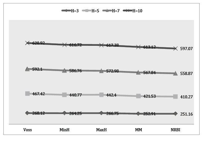
Figure 4: Average of Minimum cost found with algorithms on H=3, 5, 7, 10.

7 Conclusion

In this paper we have proposed three greedy algorithms to solve Steiner tree problem with hop constraint, which is a important class of network design. The basic ideas of first two greedy algorithms, MinHIG and MaxHIG, were limited to prim algorithm. They were good on some graphs, but we could not arrive to near optimal solution on all kind of graphs. In fact, the structure of graphs has effect on these algorithms’ solutions, since the algorithms are root based. Furthermore, we proposed an algorithm ,NRBI, which expand the idea of Kruskal algorithm. The algorithm seemed to be quite robust even when more generalized problems are considered, such as having different hop constraints for all basic vertices. In addition, some comprehensive analysis of all proposed algorithms and the comparison to the Voss’s algorithm has been shown that NRBI algorithm arrived to best solution almost in all cases. The improvement is significantly 34.60$\%$ in the best case when hop is 10 on dense graphs and in the worst case 3.34$\%$ for hop 3 on sparse graphs on these problems. An interesting future work could be use of heuristic algorithms to try to improve the feasible solutions of the proposed greedy algorithms.

References

- (1) Balakrishnan A, Altinkemer K. Using a hop-constrained model to generate alternative communication network design. ORSA Journal of Computing 4, 1992; 192-205.
- (2) Costa AM, Cardon JF, Laporte G. Models and branch-and-cut algorithms for the Steiner tree problem with revenues budget and hop constraints. Networks 2009; 53(2):141-159.
- (3) Costa AM, Cordeau J, Laporte G. Fast heuristics for the Steiner tree problem with revenues, budget and hop constraints. European Journal of Operational Research 2008. 68-78.
- (4) Kruskal B. The Shortest spanning subtree of a graph and the Traveling Salesman Problem. In: Proceedings of the American Mathematical Society. 1956. 48–50.
- (5) Duin C, Voss S. Steiner tree heuristics – A survey. In: H. Dyckoff et al. (Hrsg): Operations Research Proceedings, Springer, Berlin u.a., 1993, 485- 496.
- (6) Dahl G, Gouveia L, Requejo C. Formulations and methods for the hop-constrained minimum spanning tree problem. In: P. M. Pardalos and M. Resende, editors, Handbook of Optimization in Telecommunications, 2006, 493-515. Springer.
- (7) Akgun I, Tansel BC. Degree constrained minimum spanning tree problem: New formulation via Miller-Tucker-Zemlin constraints. Research Report, Bilkent University, Department of Industrial Engineering, Bilkent, Ankara 2009.
- (8) Ljubic I, Gollowitzer S. Layered Graph Approaches to the Hop constrained Connected Facility Location Problem, INFORMS Journal on Computing, vol. 25 no. 2013; 2 256-270.
- (9) Beasley JE. In., Distributing test problems by electronic mail. Journal of the Operational Research Society, 1990; 1072-1069.
- (10) De Boeck J. Fortz B., Extended formulation for hop constrained distribution network configuration problems. European Journal of the Operational Research Society, 2018; 488-502.
- (11) Gouveia L. Multicommodity flow models for spanning with hop constraints. European Journal of Operational Research; 1996. 178-190.
- (12) Gouveia L. Using variable redefinition for computing lower bounds for minimum spanning and Steiner trees with hop constraints. INFORMS Journal on Computing, 1998; 10(2):180-188.
- (13) Gouveia L. Using hop-index models for constrained spanning and Steiner tree models. In: B. Sanso and P. Soriano, editors, Telecommunications network planning; 1999. 21-32.
- (14) Gouveia L. Using the Miller-Tucker-Zemlin constraints to formulate a minimal spanning tree problem with hop constraints. Computers Operations Research, 1995; 22(9): 959-970.
- (15) Gouveia L, Magnanti TL. Network flows models for designing diameter-constrained minimum spanning and Steiner trees. Networks 41, 2003; 159-173.
- (16) Gouveia L, Leitner M, Ljubić I. On the Hop Constrained Steiner Tree Problem with Multiple Root Nodes. Combinatorial Optimization Lecture Notes in Computer Science 2012; 201-212.
- (17) Gouveia L, Paissa A, Sharmab D. Modeling and solving the rooted distanceconstrained minimum spanning tree problem. Computers and Operations research Lecture, 2008; 35: 600-613.
- (18) Leblance L, Chifflet J, Mahey P. Packet routing in telecommunication networks with path and flow restrictions. INFORMS Journal in Computing 11, 1999; 188-197.
- (19) Leblance L, Reddoch R. Reliable link topology/capacity design and routing in backbone telecommunications networks. Working paper, Vanderbilt University, presented at 1st ORSA SIG Conf. on Telecommunications, 1990.
- (20) Leblance L, Reddoch R, Chifflet J, Mahey P. Routing in telecommunication networks with flow restrictions. Working paper, Vanderbilt University, 1995.
- (21) Maculan N.The Steiner problem in graphs. Annals of Discrete Mathematics, 1987; 31: 185-212.
- (22) Prim RC. Shortest connection networks and some generalizations, Bell syst. Techn. J. 1957; 36:1389-1401.
- (23) Voss S. Steiner′s problem in graphs: Heuristic methods, Discrete Applied Mathematics; 1992 40:45-72.
- (24) Voss S. The Steiner tree problem with hop constraint. Annals of Operations Research 1999; 321-345.
- (25) Dokeroglu T., Mengusoglu E.. A self-adaptive and stagnation-aware breakout local search algorithm on the grid for the Steiner tree problem with revenue, budget and hop constraints. Soft Comput. 2018, 22:4133?4151.