Macro detection using fluorescence detectors

Abstract

Macroscopic dark matter (aka macros) constitutes a broad class of alternatives to particulate dark matter. We calculate the luminosity produced by the passage of a single macro as a function of its physical cross section. A general detection scheme is developed for measuring the fluorescence caused by a passing macro in the atmosphere that is applicable to any ground based or space based Fluorescence Detecting (FD) telescopes. In particular, we employ this scheme to constrain the parameter space ($\sigma_{x}\mbox{ vs}\mbox{ M}_{x}$) of macros than can be probed by the Pierre Auger Observatory and by the Extreme Universe Space Observatory onboard the Japanese Experiment Module (JEM-EUSO). It is of particular significance that both detectors are sensitive to macros of nuclear density, since most candidates that have been explored (excepting primordial black holes) are expected to be of approximately nuclear density.

1 Introduction

If General Relativity is correct, then dark matter constitutes most of the mass density of the Galaxy. While dark matter is widely thought to exist (although see [1]) we have yet to detect it except gravitationally.

The most widely considered and searched for candidates are new particles not found in the Standard Model of particle physics, such as the generic class of Weakly Interacting Massive Particles (WIMPs) (especially the Lightest Supersymmetric Particle) and axions. Recently, renewed attention has been paid to primordial black holes and to macroscopic composite objects, aka macros, especially those of approximately nuclear density. The theoretical motivation for this stems originally from the work of Witten [2], and later, more carefully Lynn, Nelson and Tetradis [3], Macroscopic objects made of baryons may be stable with sufficient strangeness, and may have formed before nucleosynthesis [2, 3], thus evading the principal constraint on baryonic dark matter. One appeal of such a dark matter candidate is that there would be no need to invoke the existence of new particles to explain the observed discrepancy between gravitational masses and luminous masses in galaxies. Numerous beyond-the-Standard-Model macro candidates have also been suggested (e.g., [4]).

Recently one of us (GDS), along with colleagues, presented a comprehensive assessment of limits on such macros as a function of their mass and cross-section [5], identifying specific windows in that parameter space that were as yet unprobed. (We later refined those [6].)

Taking macros to interact with our detectors with their geometric cross section, the expected number of macro events detected by an observatory/detector with effective area $A_{ef}$ that operates continuously over an observing time $t_{obs}$ is given by

$$N_{events} =\dfrac{\rho_{{}_{DM}}}{M_{x}}A_{ef}t_{obs}v_{x}$$ (1.1)

$$=5.5\left(\frac{kg}{M_{x}}\right)\left(\frac{A_{ef}}{1000\ km^{2}}\right)\left(\frac{t_{obs}}{yr}\right)$$

where $\rho_{{}_{DM}}$ is the local dark matter density $7\times 10^{-25}\,$g cm^-3 [5], and $M_{x}$ is the mass of the macro. For the purposes of this paper, we assume macros possess a Maxwellian distribution of speeds given by

$$f(v_{x})_{MB}=\left(\frac{1}{\pi v_{vir}^{2}}\right)^{\frac{3}{2}}4\pi v_{x}^{2}e^{-\left(\frac{v_{x}}{v_{vir}}\right)^{2}},$$ (1.2)

where $v_{vir}\approx 250\,$km s^-1. This distribution is slightly modified by the motion of the Earth as described in detail in Section 6. The cumulative distribution function is then obtained by integrating the probability distribution function up to the desired value of $v_{x}$. This allows us to determine the maximum $M_{x}$ we can probe as a function of $v_{x}$.

With a minimum allowed macro mass of $55\,$g (inferred from mica[5] that has been “exposed” to the bombardment of macros for tens of millions of years) the number density, and hence flux, of macros is quite small. Thus, any plan to detect macros on human time scales (e.g., years) requires a target of very large area.

In this work, we explore the possibility that fluorescence detectors designed to detect ultra-high energy cosmic rays might be simply modified and effectively used to detect the nitrogen fluorescence caused by a macro’s passage through the atmosphere. Through elastic scattering, the macro would deposit enough energy to dissociate the molecules and ionize or excite the atoms. This results in the formation of a plasma.

Figure 1 demonstrates the concept of detection of a macro dark matter in the atmosphere by, for example, a modified version of a single Fluorescence Detector (FD) telescope of the Pierre Auger Observatory. In this example, the macro particle penetrates the atmosphere generating a narrow column of ionization within the field of view of the FD.

We show below that the size of the macro will determine the size of the resulting plasma. For large enough values of the macro cross-section $\sigma_{x}$, we find that the plasma becomes optically thick to photons and radiates as a blackbody. We analyze the optically thick and thin mechanisms separately.

As heat diffuses out of this region surrounding the macro trajectory, the ions recombine to release photons that can be detected using fluorescence detectors. However, the macro passage through the atmosphere does not create an air shower as when a high energy cosmic ray is detected. We find that for the Pierre Auger Observatory (Auger) and the proposed Extreme Universe Space Observatory onboard the Japanese Experiment Module (JEM-EUSO), we can probe masses up to 1.6$\times 10^{4}\,$g and 5.5$\times 10^{6}\,$g respectively for an observation period of 1 year, thus providing significant improvements over the current $55\,$g limit.

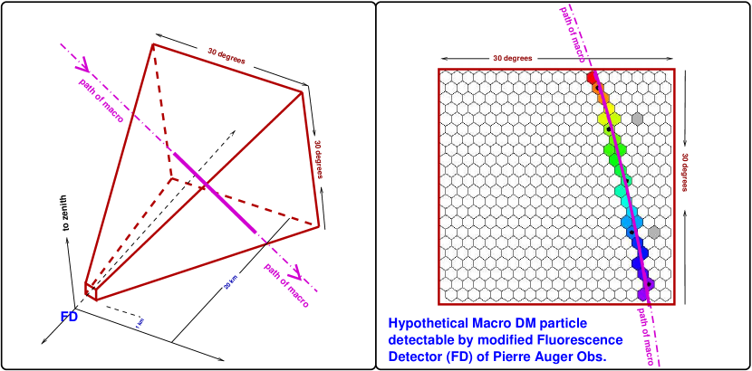
Figure 1: Conceptual diagram delineating the plausible detection of a macro dark matter particle by a modified version of a Fluorescence Detector (FD) such as that of the Pierre Auger Observatory. Left: Perspective view of the truncated pyramid corresponding to the $30^{\circ}\times 30^{\circ}$ field-of-view of a single camera (‘eye’) with a fiducial detection volume that ranges from 1 km to 20 km distance from the Auger FD. In this example, the macro particle penetrates the fiducial region at a near-vertical angle generating a perfectly straight “pencil beam” of ionized plasma. Note that in contrast to relativistic cosmic rays, a macro particle is moving much slower and will not generate an air shower. Right: Example ‘event display’ for a modified Auger FD showing the predicted appearance of a macro signal detected within the field-of-view (the linear path of the macro appears as a slightly bent line due to curvature of the FD camera focal plane). The three-dimensional path of the macro can be fully reconstructed using pixel locations and timing. A macro event is clearly distinguished from cosmic rays and other atmospheric phenomena by it’s velocity (about 250 km/s), perfectly straight path, and an ionization signal proportional to the atmospheric density.

2 Fluorescence Signal

The cross-sectional area $\sigma_{x}$ of a macro of mass $M_{x}$ and density $\rho_{x}$ is

$$\sigma_{x}=2.4\times 10^{-10}\,{\mathrm{cm}}^{2}\left(\frac{M_{x}}{g}\right)^{2/3}\left(\frac{\rho_{nuclear}}{\rho_{x}}\right)^{2/3}\,,$$ (2.1)

where we take $\rho_{nuclear}=3.6\times 10^{14}\,$g cm^-3. In this manuscript, we are interested in probing densities above $10^{6}\,$g cm^-3 up to nuclear densities, with a particular emphasis on the latter. A macro of mass greater than $55\,$g and of a density of likely interest will therefore be much larger than the separation of molecules in the atmosphere, $\sim$ few $\times 10^{-7}\,$cm. We also reasonably assume that the internal density of the macro is much larger than that of air, and that its velocity will not be significantly altered as a result of collisions with individual air molecules.

During its passage through the atmosphere, the macro will dissociate molecules, and ionize and excite atoms both by direct impact, more importantly through subsequent secondary effects of those impacts. With $v_{x}=250\,$km s^-1, after the impact of a macro with a single nitrogen molecule, that molecule will be dissociated, and the nitrogen atoms will rebound with velocities $v\lesssim 500\,$km s^-1. The kinetic energy of the rebounding atoms will result in secondary collisions with other air molecules. Since many secondary collisions are required before the energy is thermalized, these collisions will dominate the net ionization and excitation.

Following the work of Cyncynates et al. [7], we propagate the initial energy deposition by the macro, which we approximate as a delta function along a straight trajectory, outward radially away from that trajectory according to the heat equation. Ignoring radiative cooling, the temperature field after some time $t$ is

$$T(r,t)=\frac{\sigma_{x}v_{x}^{2}}{4\pi\alpha c_{p}}\frac{e^{-\frac{r^{2}}{4t\alpha}}}{t},$$ (2.2)

where $\alpha\approx 10^{-4}\,$m${}^{2}\,$s^-1exp$(D/10$km$)$ is the thermal diffusivity of the air, and $c_{p}\approx 25$ kJ kg^-1 K^-1 is the specific heat of the air [8]. (The specific heat varies around a mean of $\sim 25\,$kJ kg${}^{-1}\,$K^-1 for temperatures between $10^{4}\,$K and $10^{5}\,$K, and the corresponding thermal diffusivities vary around $0.08\,$m${}^{2}\,$s^-1.)

We invert (2.2) to obtain $\pi r_{I}(t)^{2}$, the area at time $t$ that reaches a particular state of ionization I characterized by the appropriate ionization temperature $T_{I}$, by setting $T(r,t)=T_{I}$. This area is given by

$$\pi r_{I}(t)^{2}=4\pi\alpha t\log\left(\frac{\sigma_{x}v_{x}^{2}}{4\pi\alpha tc_{p}T_{I}}\right).$$ (2.3)

After the macro passes, the ionized area starts at $0$ at $t=0$, increases to a maximum, then falls back to $0$ at

$$t_{I0}=\frac{\sigma_{x}v_{x}^{2}}{4\pi\alpha c_{p}T_{I}}\approx 20\,s\left(\frac{\sigma_{x}}{cm^{2}}\right)\left(\frac{v_{x}}{250kms^{-1}}\right)^{2}e^{-\frac{D}{10km}}.$$ (2.4)

$t_{cool}$ is defined as the time for the temperature everywhere to fall below $T_{I}=10^{4}\,$K[9] corresponding to the ionization temperature for NI. At this point nearly all the electrons will have recombined and hence $\pi r_{I}(t)^{2}=0$. In other words, $t_{cool}=t_{I0}$.

The cooling time (equation (2.4)) thus depends on the cross section $\sigma_{x}$ and the speed $v_{x}$ of the incoming macro. Typically, most incoming macros will approach at $v_{x}\sim 250\,$km s^-1. Thus the cooling time is plotted taking $v_{x}=250\,$km s^-1 and $D=1$ km, $5$ km and $20$ km respectively in Figure 2, along with the proposed bin times for Auger and JEM-EUSO to be able to detect macros. In particular, if the bin time of an FD is less than the cooling time, $t_{cool}$, the macro will cause fluorescence over multiple time bins. We proceed to calculate the number of photons produced during this interval.

The formation of a plasma with a definite temperature field will not hold for macros of a small $\sigma_{x}$ which would be unable to impart sufficient energy to a large number of nitrogen molecules. The (internal) energy fluctuates randomly about the mean value. This statement can be quantified by the thermal fluctuations, which are given by

$$\left(\frac{\langle(E-\langle E\rangle)^{2}\rangle}{\langle E\rangle^{2}}\right)\sim N^{-\frac{1}{2}}$$ (2.5)

The quantity N is determined by the causal volume of the resulting plasma, i.e. $N=\sigma_{x}n_{a}L$, where $L=c_{s}t_{I0}$ and $c_{s}\approx 300\,$m s^-1 is the speed of the sound in air. By requiring that the thermal fluctuations do not exceed $10\%$, i.e. $N\geq 100$, we find $\sigma_{x}\gtrapprox 3\times 10^{-12}$ cm² will produce a plasma. This sets a lower bound on the sensitivity of an FD to detect macros.

All subsequent analysis will be to determine if an FD can reach this lower limit. Each FD produces an effective volume that relates the height, D, away from the pixels to the maximum mass, $M_{x}$ that FD can probe at that particular height. In other words, $M_{x}(D)$ for a given integration time. Such a relationship allows us to relate $\sigma_{x}$ to $M_{x}$ to quantify a lower bound that can be plotted on 8. This analysis is done for two particular FDs in section 4.

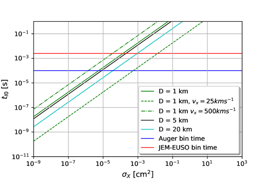
Figure 2: Cooling time as a function of macro cross section $\sigma_{x}$. The two horizontal lines represent the proposed bin times for Auger and JEM-EUSO to be able to detect macros.

An important distinction needs to be made regarding the opacity of the resulting plasma along the macro trajectory. For large enough $r_{I}$, the plasma becomes optically thick. For the temperatures of interest ($\geq 10^{4}\,$K), the scattering length of air is a few meters [10].

To obtain the value of $\sigma_{x}$ demarcating the transition between an optically thick and thin plasma, we first find the maximum area that achieves each specific degree of ionization

$$\pi r_{I,max}^{2}=4t_{I,max}\alpha\pi=\frac{\sigma_{x}v_{x}^{2}}{c_{p}T_{I}e}\,,$$ (2.6)

reached at $t_{I,max}=t_{I0}/e$. The $T_{I}$ of interest corresponds to that of NII.

We compare $r_{I,max}$ and the scattering length $\lambda_{sc}$, which is dependent on the number density of the atoms and hence the height above the ground

$$\lambda_{sc}=\lambda_{sc,0}e^{\frac{D}{10\,km}}$$ (2.7)

where $\lambda_{sc,0}$ is the scattering length for the number density of the atoms at ground level. Using (2.7) in (2.6), we find that only large macros with cross sections at the upper limits of the unprobed parameter space could plausibly produce a large enough column of plasma that would emit as a blackbody in the optically thick regime, i.e macros that satisfy

$$\left(\frac{\sigma_{x}}{cm^{2}}\right)\left(\frac{v_{x}}{250km\,s^{-1}}\right)^{2}\geq e^{\frac{D}{5\,km}}22000$$ (2.8)

For completeness, we present that case separately from the optically thin emission mechanism below.

Another important consideration is the relationship between the recombination timescales of the electrons through three-body recombination, radiative recombination and spontaneous emission. To the best of our knowledge, the rates that exist in the literature are from very low electron number densities that are not applicable to our analysis. The NII rates, however, are available for reasonably high electron number densities. Using the rates from [11] (and also see references therein) we find that approximately $10^{-6}$ electrons will recombine radiatively. In [11] these rates were calculated for both an optically thick and thin plasma. The optically thin calculation depends on both the electron temperature and number density(see Figures 8 and 9 of [11]). The rates thus depend on the atmospheric depth through the number density of electrons. The discrepancies in these quantities with experiments are approximately a factor of 2 [11] and thus we expect corrections to be of order $\sim 1$ to the SNR values calculated below. We account for this below when we calculate the number of photons emitted through a factor

$$\beta_{1}=\frac{\alpha_{rad}}{k_{three}n_{e}}=10^{-6}$$ (2.9)

that represents the fraction of electrons that recombine radiatively for the first ionization state. We have used the three-body recombination coefficient for $n_{e}=10^{22}\,$m^-3. This is an underestimate of the true value of $\beta_{I}$ because the coefficient decreases with increasing $n_{e}$. However, reference [11] only obtained the three-body recombination coefficient up to $n_{e}=10^{22}\,$m^-3.

For photons free-streaming from the optically thin plasma, i.e. $r_{I,max}<\lambda_{sc}$, we must also compare the “recombination time” of the plasma $t_{rec}$ to its “cooling time” $t_{cool}$. If $t_{rec}\leq t_{cool}$, each electron can contribute multiple photons through multiple ionizations and recombinations.

The radiative recombination rate coefficient is approximately constant across the temperature range of interest [11], $\alpha_{rad}\approx 4\times 10^{-19}\,$m${}^{3}\,$s^-1. Thus

$$t_{rec}\equiv\frac{1}{n_{e}\cdot\alpha_{rad}}\simeq 3\times 10^{-8}s\ e^{\frac{D}{10\,km}},$$ (2.10)

with $n_{e}=n_{e,0}exp(-D/10$km$)$ and $n_{e,0}\approx 10^{26}\,$m^-3 is the electron number density at ground level.

Comparing $t_{rec}$ with $t_{cool}$, we find

$$\left(\frac{\sigma_{x}}{cm^{2}}\right)\geq 10^{-9}\,e^{\frac{D}{5\,km}}\left(\frac{250\,km\,s^{-1}}{v_{x}}\right)^{2}.$$ (2.11)

For the values of $\sigma_{x}$, $v_{x}$ and D of interest, we find that macros in the parameter space we seek to probe would produce a plasma where each electron will recombine multiple times.

To account for this, we multiply the expression for the number of photons produced per unit length $\frac{dN}{dl}\gamma$ by a quantity $N_{mult}=\min\left(1,\frac{t_{cool}}{t_{rec}}\right)$.

To find the number of photons that reach a detector pixel, we first estimate the electron number density in the recombining plasma, by using (2.3) for $t_{I0}/e\leq t\leq t_{I0}$. We can then find the number of photons emitted during recombination. We multiply by the transverse distance L $=$ D sin$\theta$(we justify this choice for L in section 5) traveled by the macro across the field of view of a pixel (where D is the height of the macro path above the detector and $\theta$ is the angle viewed by the pixel) and by the ratio of the detector area to the area of a sphere of radius D,

$$N_{\gamma}=\derivative{N}{l}\left(\frac{A_{detector}}{4\pi D^{2}}\right)L=\derivative{N}{l}\left(\frac{A_{detector}\sin\theta}{4\pi D}\right).$$ (2.12)

For the free streaming case, photon production happens on a timescale $t_{I0}$. A Fluorescence Detector (FD) telescope integrates over small intervals, known as the bin time, $\tau_{bin}$. For the $\tau_{bin}$ we consider below, $t_{I0}<\tau_{bin}$ for all $\sigma_{x}$. Consequently the number of photons emitted per unit length along the macro path trajectory in one bin time is

$$\derivative{N}{l} =2N_{mult}\eta\pi\int_{\frac{t_{I0}}{e}}^{t_{I0}}\int_{0}^{r_{I}(t)}\beta_{1}n_{e1}n_{a}\alpha_{rad}rdrdt$$ (2.13)

$$\approx 2N_{mult}\times 10^{-8}s^{2}\alpha\eta n_{a}^{2}\alpha_{rad}\left(\frac{\sigma_{x}}{cm^{2}}\right)^{2}\left(\frac{v_{x}}{250\,kms^{-1}}\right)^{4}$$

We have introduced in (2.13) the quantity $\eta$, which is the probability that transitions in a nitrogen plasma produce a photon in the $350-400\,$nm detection range. This is important as the detectors considered below are sensitive only within this waveband. This value was obtained from the ratio of Einstein coefficients of transitions that resulted in wavelengths within our range to the Einstein coefficients of all transitions (using tabulated data from [12])

$$\eta=\frac{\sum\nolimits_{350-400nm}A_{ki}}{\sum\nolimits_{all}A_{ki}},$$ (2.14)

where $A_{ki}$ is the Einstein coefficient for a transition from a state i to a state k. We find $\eta\approx 2\times 10^{-3}$.

The quantity $N_{mult}$ is given as

$$N_{mult}=\frac{\rho_{0}\sigma_{x}v_{x}^{2}\alpha_{rad}n_{e0}e^{-\frac{D}{5}}}{4\pi KT_{1}}=6\times 10^{8}\left(\frac{\sigma_{x}}{cm^{2}}\right)\left(\frac{v_{x}}{250\,km\,s^{-1}}\right)e^{-\frac{D}{5\,km}}$$ (2.15)

Evaluating (2.12) using (2.13) and (2.15), the number of photons received in a detector pixel in one bin time in the case of the optically thin plasma is

$$N_{\gamma}^{thin}=3\times 10^{27}\min\!\left(\frac{\tau_{bin}}{t_{I0}},1\right)\frac{A_{detector}\sin\theta}{D\leavevmode\nobreak\ km}\left(\frac{\sigma_{x}}{cm^{2}}\right)^{3}\left(\frac{v_{x}}{250\,km\,s^{-1}}\right)^{6}e^{-\frac{2D}{5\,km}}\,$$ (2.16)

where $A_{detector}$ and D have units of km²(as will be the case throughout this analysis). The factor $\min\!\left(\frac{\tau_{bin}}{t_{I0}},1\right)$ accounts approximately for the case where $\tau_{bin}\leq t_{I0}$, with the precise value of $N_{\gamma}^{thin}$ depending on when exactly the light from the macro path enters the pixel.

Since we ignored radiative cooling when solving the heat equation, we calculate the fraction of the energy deposited by the macro that we have attributed to photon emission to ensure that we do not violate energy conservation

$$\frac{E_{freestream}}{E_{initial}} =\frac{\mbox{N}_{\gamma}^{thin}\overline{E}}{\frac{1}{2}\rho_{atm}(v_{x})^{2}\sigma_{x}\mbox{L}}$$ (2.17)

$$\approx 2\times 10^{5}\left(\frac{\sigma_{x}}{cm^{2}}\right)^{2}\left(\frac{v_{x}}{250\,km\,s^{-1}}\right)^{4}e^{-\frac{2D}{5\,km}},$$

For $\left(\frac{\sigma_{x}}{cm^{2}}\right)^{2}\left(\frac{v_{x}}{250\,km\,s^{-1}}\right)^{4}\gtrapprox\frac{1}{2\times 10^{5}}$,this implies a violation of energy conservation that may be traced back to the failure to include radiative losses in the solution (2.2) of the heat equation. (As appropriate in the context of [7].) The value of $N_{\gamma}^{thin}$ from (2.16) should not be trusted but would instead be expected to approximately saturate at the level

$$N_{\gamma}^{thin}=3\times 10^{19}\frac{A_{detector}\sin\theta}{D\leavevmode\nobreak\ km}\,\min\left(10^{8}\left(\frac{\sigma_{x}}{cm^{2}}\right)^{3}\left(\frac{v_{x}}{250\,km\,s^{-1}}\right)^{6}e^{-\frac{2D}{5\,km}},1\right)\min\!\left(\frac{\tau_{bin}}{t_{I0}},1\right)$$ (2.18)

We now proceed to examine the blackbody emission case. We integrate the Planck spectrum over the wavelengths of interest to find the number of photons emitted by the plasma per unit length along the macro trajectory

$$\derivative{N}{l} =\int_{0}^{t_{cool}}\int_{\nu_{350nm}}^{\nu_{400nm}}\frac{4\pi 2\pi r{\tiny{}_{10000K}}(t)}{h\nu}B(\nu,T)d\nu dt$$ (2.19)

$$=3.0\times 10^{27}\frac{1}{km}\left(\frac{\sigma_{x}}{cm^{2}}\right)^{3/2}\left(\frac{v_{x}}{250\,km\,s^{-1}}\right)^{3}$$

From (2.12) and (2.19), we get $N_{\gamma}^{thick}$ just as in the free-streaming case

$$N_{\gamma}^{thick}=2\times 10^{26}\min\!\left(\frac{\tau_{bin}}{t_{I0}},1\right)\frac{A_{detector}\sin\theta}{D\leavevmode\nobreak\ km}\left(\frac{\sigma_{x}}{cm^{2}}\right)^{3/2}\ \left(\frac{v_{x}}{250\,km\,s^{-1}}\right)^{3}$$ (2.20)

We similarly calculate the energy fraction that is emitted as photons for the blackbody scenario by

$$\frac{E_{bb}}{E_{initial}}\approx 0.4\left(\frac{\sigma_{x}}{cm^{2}}\right)^{\frac{1}{2}}\left(\frac{v_{x}}{250kms^{-1}}\right)$$ (2.21)

For $\left(\frac{\sigma_{x}}{cm^{2}}\right)^{\frac{1}{2}}\left(\frac{v_{x}}{250\,km\,s^{-1}}\right)\gtrapprox 1$, this implies a violation of energy conservation as in the case of the optically thin solution. Additionally, the value of the cooling times, $t_{I0}$ are much longer than the bin time that the factor $\min\!\left(\frac{\tau_{bin}}{t_{I0}},1\right)$ is always given by $\frac{\tau_{bin}}{t_{I0}}$. The value of $N_{\gamma}^{thick}$ from (2.20) would be expected to saturate at

$$N_{\gamma}^{thick}=3\times 10^{24}\frac{A_{detector}\sin\theta}{D\leavevmode\nobreak\ km}\times\frac{\tau_{bin}}{t_{I0}}$$ (2.22)

where we have taken $\left(\frac{\sigma_{x}}{cm^{2}}\right)^{\frac{1}{2}}\left(\frac{v_{x}}{250\,km\,s^{-1}}\right)\approx 1$ from (2.21). The blackbody regime exists entirely above the $\sigma_{x}v_{x}^{2}$ cutoff from (2.21).

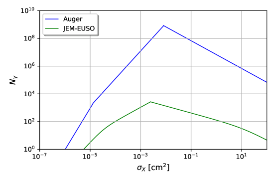
Figure 3: The expected number of photons received at the detector as a function of $\sigma_{x}$ for Auger(green) taking D$=10\,$km and JEM-EUSO(black) taking D$=400\,$km as predicted in section 4.1. The choice of D $=10$ km for Auger is explained in section 4.1.

(2.18) and (2.22) are multi-valued depending on the value of $\sigma_{x}$ and $v_{x}$. For large enough or sufficiently quick macros, a pixel can be lit up for multiple time bins. In addition to that, the amount of photons produced levels off for sufficiently large or high speed macros. For both detectors considered in this work, the transition to pixels being lit up for multiple time bins occurs prior to the leveling off. In Figure 3, we plot (2.16) and (2.22) for both Auger(with a characteristic D$=10\,$km) and JEM-EUSO across the entire range of $\sigma_{x}$ we hope to probe. We provide detector specific quantities used in this calculation in (2.16) and (2.22) in section 4 below.

Since we have solved for the number of photons produced in the optically thick and thin cases separately, we find that the solutions do not smoothly transition (2.8). Thus, we interpolated the optically thin solution at the transition points. We expect that after 3 scattering lengths that thermalization will occur and the optically thick regime is thus set at $9\sigma_{x,FS}$, where $\sigma_{x,FS}$ is the transition cross section for a fixed $v_{x}$.

In the following section, we discuss the signal-to-noise ratio.

3 Detection Signal-to-Noise

In the previous section, we calculated the number of photons $N_{\gamma}$ produced by the macro in the detector waveband that reach a detector pixel. To ensure an FD telescope can detect the macro requires that the signal produced by those photons exceed the noise due to the background, i.e. we require that the signal-to-noise ratio (SNR)

$$\mbox{SNR}=\dfrac{Q\ FN_{\gamma}}{N_{noise}}\,,$$ (3.1)

exceed some threshold value.

As we see in (3.1), the signal consists of the the number of photons incident on the detector $N_{\gamma}$ multiplied by the photomultiplier tube (PMT) quantum efficiency factor $Q$ – the fraction of photons averaged over the appropriate waveband that enter the detector and go on to produce photoelectrons and so result in a signal and $F$, the fraction of photons that survive the attenuation due to Mie and Rayleigh scattering as the photons travel towards the detector. $Q$ varies among detectors. Here $Q$ is taken to be 0.2 and $F$ is taken to be 0.5, conservatively. The noise can be modeled as a Poisson distribution with contributions from the source and the background

$$N_{noise}=(Q(FN_{\gamma}+N_{background}))^{\frac{1}{2}}\,,$$ (3.2)

where

$$N_{background}=\Phi_{background}A_{detector}\tau_{bin}\Omega_{pix}.$$ (3.3)

Here $\Phi_{background}$ is the number of background photons per unit area per unit time per unit solid angle and $\Omega_{pix}$ is the solid angle subtended by a pixel. If

$$\frac{Q\ FN_{\gamma}}{N_{Noise}}\geq\mbox{SNR}_{min}$$ (3.4)

we can detect a macro. As is customary, we take $\mbox{SNR}_{min}=5$.

A combination of (1.1), (2.16), (2.22) and (3.4), applied to a particular FD telescope gives us the parameter space of macros that can be probed by that FD. In particular, we compare $N_{\gamma}$ with $N_{noise}$ and determine the range of $\sigma_{x}$ for which (3.4) holds. We then determine the mass range that can be probed from the expected event rate in that FD.

4 Specific examples

We apply the above detection scheme to two specific examples, representing two main variants of fluorescence detection telescopes: the existing Auger Fluorescence Detector – a ground-based fly’s eye type instrument – and the planned JEM-EUSO Fresnel-lens based space telescope.

4.1 Pierre Auger Observatory

The Pierre Auger Observatory [13, 14] includes 24 Fluorescence Detector (FD) telescopes. Each telescope is composed of 22$\times$ 20 pixels covering a 30$\degree\times$ 30$\degree$ field of view [15] out to a range of approximately 20 km. Each telescope thus observes a fiducial volume corresponding to a flat-sided pyramid a square base with sides $2\times\sin{15\degree}\times$ 20 km$\approx 10^{4}\,$m. We ignore the first km of the cone nearest the telescope, as the time evolution of the intensity of the ionization source as it moves through the atmosphere, will show no significant variation from which to draw useful information. We chose a characteristic quantum efficiency $Q$ =20% corresponding to an average over the detected fluorescence wavelengths [25].

The Auger detector was designed to look for relativistic cosmic ray particles. The bin time was therefore set at $\tau_{bin}=100\,$ns, during which time an ultra relativistic cosmic ray would travel approximately $30\,$m, but a macro would traverse only a few cm. For the much more slowly moving macros, we will need to increase this to $\tau_{bin}=100\,\mu\,$s. This reconfiguration might require both software and hardware changes to the FD telescope and/or trigger system.

The analysis undertaken in section 2 was to determine the detectability of a passing macro in one pixel. To ensure that a passage of a macro will trigger at least 4 pixels in a row, we take a reduced detector volume by ignoring the outer 3 pixels in our array. This reduces the detector volume in Auger by a factor of $\frac{17\times 19}{20\times 22}\approx 0.73$.

Since we consider an isotropic flux we must account for all possible paths within this detection volume. The effective target area averaged over all angles for a single FD telescope is $120\,$km². Running the detector for an observation period of 1 year ($\sim$ 10 years with the Auger FDs characteristic 10$\%$ duty cycle[15]) yields an expected number of events

$$N_{events}^{1FD}=\left(\frac{g}{M_{x}}\right)\left(\frac{D_{max}(\sigma_{x})}{km}\right)^{2}\,.$$ (4.1)

where $D_{max}(\sigma_{x})$ represents the maximum distance away we could detect a macro of a particular cross section. The minimum height below which no new parameter space can be probed is D$\approx 5.8\,$km. For heights below this, the effective target area of the detector is too small to extend above 55 g, below which all values of $\sigma_{x}$ has been ruled out(see Figure 8) through CMB and mica measurements[5]. The cost of probing higher masses, $M_{x}$, at higher values of D is a reduced sensitivity in $\sigma_{x}$ because of geometrical spreading. Thus, we choose D$=10$km in plotting Figure 3 to illustrate the expected SNR for macros in unconstrained parameter space.

We might be able to probe masses up to 660 g with one Auger FD telescope. If the entire Auger FD array could be used, the effective target area becomes $3\times 10^{3}\,$km². This pushes the upper mass accessible to $1.6\times 10^{4}\,$g. Another $50\,\%$ improvement could be obtained if the duty cycle could be improved to $\sim 15\,\%$, as has been claimed [16].

R. Caruso et. al [17] measured the background sky photon flux at two FD telescope sites at Malargüe: Los Leones and Coihueco. Using (3.3) and taking their highest measured background value of $\Phi_{background}=134\,$m${}^{-2}\,$deg${}^{-2}\,\mu$s^-1,

$$N_{background}^{1FD} \approx 4\times 10^{5}$$ (4.2)

(for $A_{detector}\approx 13\,$m² [18], $\tau_{bin}=100\,\mu$s and $\Omega_{pix}=(1.5\degree)^{2}$).

Using (2.16), (3.1), (3.2) and (4.2) we find that

$${\small SNR_{FS,Auger}^{1FD}}= \sqrt{\frac{3\times 10^{20}\left(\frac{km}{D}\right)\left(\frac{\sigma_{x}}{cm^{2}}\right)^{3}e^{-\frac{2D}{5\,km}}}{1+8\times 10^{-16}\frac{D}{km}\left(\frac{cm^{2}}{\sigma_{x}}\right)^{3}e^{\frac{2D}{5\,km}}}}, \begin{split}{\small\text{\mbox{\bf FSU}}}\end{split}$$ (4.3a)

$${\small SNR_{FS,Auger}^{1FD}}= \sqrt{\frac{2\times 10^{15}\left(\frac{km}{D}\right)\left(\frac{\sigma_{x}}{cm^{2}}\right)^{2}e^{-\frac{3D}{10\,km}}}{1+2\times 10^{-10}\frac{D}{km}\left(\frac{cm^{2}}{\sigma_{x}}\right)^{2}e^{\frac{3D}{10\,km}}}}, \begin{split}{\small\text{\mbox{\bf FSUT}}}\end{split}$$ (4.3b)

$${\small SNR_{FS,Auger}^{1FD}}= \sqrt{\frac{2\times 10^{7}\left(\frac{km}{D}\right)\left(\frac{\sigma_{x}}{cm^{-1}}\right)^{2}e^{\frac{D}{10\,km}}}{1+2\times 10^{-2}\frac{D}{km}\left(\frac{cm^{2}}{\sigma_{x}}\right)^{-1}e^{-\frac{D}{10\,km}}}}, \begin{split}{\small\text{\mbox{\bf FSST}}}\end{split}$$ (4.3c)

where we have set $v_{x}=250$kms^-1 to simplify the process of producing Figure 4. We will discuss how reasonable is this assumption in section 5. Here we use the labels corresponding to the different emission mechanisms and instrumental constraints: FS=”Free-Streaming”, FSUT=”Free Streaming Unsaturated with $\tau_{bin}<t_{I0}$” and FSST=”Free Streaming Saturated with $\tau_{bin}<t_{I0}$”. These ranges and expected sensitivities are also summarized in Table 1.

Using the expressions for the SNR, one can(for various values of D), by setting $SNR\geq 5$ for detection obtain the range of $\sigma_{x}$ that can be probed by Auger. We plot the SNR in Figure 4 for various values of D(km) for which detection is possible using the FDs of Auger. Although the expression for the SNR is labeled as applying only to 1 FD, it is also relevant to the entire array. Utilizing the entire array increases in the upper bound of masses that may be probed, which in turn increases the sensitivity to macro cross section because of a reduction in geometric spreading of the signal.

To determine the form the lower bound of the one-telescope purple region in Figure 8, we have iterated over various values $\sigma_{x}$ For each value of $\sigma_{x}$, we have iterated over various $v_{x}$ values and determined the maximum value of D(km) that a macro of the given $\sigma_{x}$ can be detected. For each $v_{x}$, the fraction of macros that would possess that speed is determined and this quantity multiplied to determine the through value of $M_{x}$ that can be probed by Auger. The highest $M_{x}$ for a given $\sigma_{x}$ was used in plotting Figure 8.

For the full Auger FD array, the lower boundary is of the same form that of the one FD bound, with the exception being that we can probe up to $1.2\times 10^{4}\,$g instead of $480\,$g. A similar analysis was done as in the one FD case. The lower bound of the entire array region in Figure 8 is the sum of the striped and non-striped purple regions.

For the optically thick (black body) case using (2.22), (3.1), (3.2) and (4.2) we have for both a single FD telescope and the entire array

$$SNR_{BB,Auger}^{1FD}=\sqrt{\frac{2\times 10^{12}\left(\frac{km}{D}\right)\left(\frac{\sigma_{x}}{cm^{2}}\right)^{-1}e^{\frac{D}{10\,km}}}{1+2\times 10^{-7}\frac{D}{km}\left(\frac{cm^{2}}{\sigma_{x}}\right)^{-1}e^{-\frac{D}{10\,km}}}}$$ (4.4)

We have not shown the expressions for the transition between the optically thin and thick emission mechanisms because the interpolation must be done for specific values of D. For Auger, the BB emission mechanism lies beyond the range of parameter space that can be probed. We plot the above expressions in Figure 4.

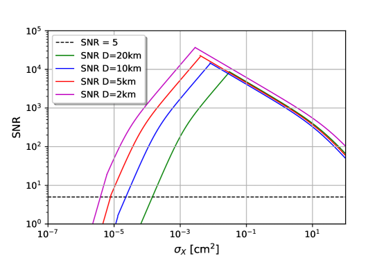
Figure 4: SNR as a function of $\sigma_{x}$ for various values of D(km) for Auger.

In the following subsection, we repeat the calculations done for Auger above for JEM-EUSO.

4.2 JEM-EUSO

JEM-EUSO is a planned Ultra-High Energy Cosmic Ray (UHECR, $E>10^{18}\,$eV) detector to be placed in the Japanese Experiment Module of the International Space Station. It will watch the dark-side of the Earth and detect UV photons emitted in extensive air showers caused by UHECRs, and especially Extremely High Energy Cosmic Ray (EHECR) particle ($E\gtrapprox 10^{20}$ eV). The telescope will have approximately $200,000$ pixels, a detection distance from space to Earth’s surface of 400 km, and an angular resolution of $0.07\degree$. This gives a fiducial cone with $L\simeq 750\,$m at the ground. The planned JEM-EUSO binning time [19] is $\tau_{bin}^{EUSO}=2.5\,\mu$s. As is the case for Auger, the JEM-EUSO binning time will need to be increase by a factor of 1000 to a value of $2.5\,$ms for the macro search. We take D$=400$km because using a smaller D would reduce the strength of the signal as the signal depends strongly on the electron number density even though there is a reduced distance between the source and detector.

JEM-EUSO will also be able to operate in “tilt” mode, looking not straight down at the Earth but at an angle to the nadir. This will increase the effective area markedly. Though the consequence of this have yet to be fully explored [20], we will proceed with $A_{ef}\sim 10^{6}\,$km², appropriate to a tilt angle of $40\degree$ (see Figure 5 of [21]). Equation (1.1) gives, for one year of JEM-EUSO observations,

$$N_{events}\simeq\frac{6\times 10^{6}g}{M_{x}}\,,$$ (4.5)

allowing us to probe masses up to $6\times 10^{6}\,$g.

Meanwhile, based on [22] and [23], $\Phi_{background}=600\,$m${}^{-2}\,$sr${}^{-1}\,$ns^-1, $A_{detector}\approx 5\,$m² , $\tau_{bin}=2.5\,$ms and $\Omega_{pix}=(0.07\degree)^{2}$, yielding

$$N_{background} \approx 10^{4}.$$ (4.6)

Using (2.16), (3.1), (3.2) and (4.6), we find that

$${\small SNR_{FS,JEM}^{1FD}}= \sqrt{\frac{3\times 10^{20}\left(\frac{km}{D}\right)\left(\frac{\sigma_{x}}{cm^{2}}\right)^{3}e^{-\frac{2D}{5\,km}}}{1+2\times 10^{-17}\frac{D}{km}\left(\frac{cm^{2}}{\sigma_{x}}\right)^{3}e^{\frac{2D}{5\,km}}}}, \begin{split}{\small\text{\mbox{\bf FSU}}}\end{split}$$ (4.7a)

$${\small SNR_{FS,JEM}^{1FD}}= \sqrt{\frac{2\times 10^{15}\left(\frac{km}{D}\right)\left(\frac{\sigma_{x}}{cm^{2}}\right)^{2}e^{-\frac{3D}{10\,km}}}{1+4\times 10^{-12}\frac{D}{km}\left(\frac{cm^{2}}{\sigma_{x}}\right)^{2}e^{\frac{3D}{10\,km}}}}, \begin{split}{\small\text{\mbox{\bf FSUT}}}\end{split}$$ (4.7b)

$${\small SNR_{FS,JEM}^{1FD}}= \sqrt{\frac{2\times 10^{7}\left(\frac{km}{D}\right)\left(\frac{\sigma_{x}}{cm^{-1}}\right)^{2}e^{\frac{D}{10\,km}}}{1+4\times 10^{-4}\frac{D}{km}\left(\frac{cm^{2}}{\sigma_{x}}\right)^{-1}e^{-\frac{D}{10\,km}}}}, \begin{split}{\small\text{\mbox{\bf FSST}}}\end{split}$$ (4.7c)

To obtain the exclusion region in 8, $D=400$km was used. For various values of $v_{x}$, the minimum $\sigma_{x}$ that was detectable was obtained and the corresponding $M_{x}$ found using the fraction of macros having the minimum speed $v_{x}$.

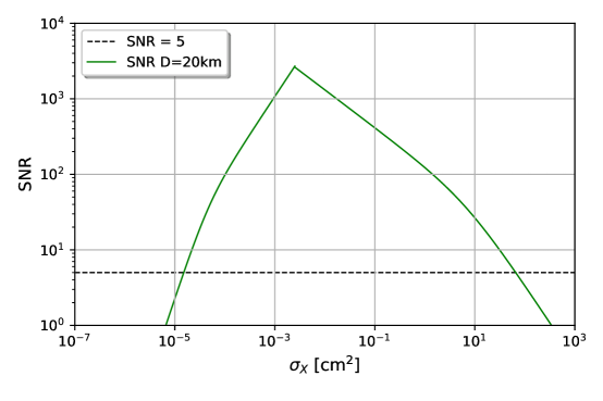
Figure 5: SNR as a function of $\sigma_{x}$ for $D=400\,$km for JEM-EUSO.

For the blackbody spectrum, we find that (2.22), (3.1), (3.2) and (4.6) gives

$$SNR_{BB,JEM}^{1FD}=\sqrt{\frac{2\times 10^{12}\left(\frac{km}{D}\right)\left(\frac{\sigma_{x}}{cm^{2}}\right)^{-1}e^{\frac{D}{10\,km}}}{1+4\times 10^{-9}\frac{D}{km}\left(\frac{cm^{2}}{\sigma_{x}}\right)^{-1}e^{-\frac{D}{10\,km}}}},$$ (4.8)

Again, we use the labels corresponding to the different emission mechanisms and instrumental constraints: FS=”Free-Streaming”, FSUT=”Free Streaming Unsaturated with $\tau_{bin}<t_{I0}$” and FSST=”Free Streaming Saturated with $\tau_{bin}<t_{I0}$”. These ranges and expected sensitivities are also summarized in Table 2.

We plot $SNR_{BB,JEM}$ in Figure 5.

In Figure 8 below, we show how the regions of parameter space that could potentially be probed by Auger and JEM-EUSO fit into the existing constraints on the macro parameters from [7].

It is of particular significance that both detectors are sensitive to macros of nuclear or lower density, since the expected Standard Model macro candidates, as well as most others that have been explored (excepting primordial black holes), are expected to be of approximately nuclear density (see e.g. [4]).

5 Discussion

In this section, we review some of the assumptions made in the preceding analysis.

We begin with the assumption that $L=Dsin\theta$. $L$ is dependent on the inclination of the macro trajectory $i$, the polar angle $\phi$ and the height $D$.

From geometrical considerations, we find

$$L=2D\frac{sin\left(\frac{\theta}{2}\right)}{cos(\frac{\theta}{2}-i)}(1+cos\theta^{2}tan(\phi)^{2})^{\left(\frac{1}{2}\right)}$$ (5.1)

A Monte Carlo simulation was done by sampling values of $\phi$ and $i$. The results were compared to the quantity $Dsin\theta$. Approximately three quarters of the trajectories had a $1\leq\frac{L}{Dsin\theta}\leq 4$. With most of the trajectories being clustered around the quantity $Dsin\theta$, we used $L=Dsin\theta$ to simplify our calculations of the SNR.

This produces an underestimate of the true SNR because we are approximating the entirety of photon production at distances greater than the true production. For macro trajectories with $L\gg Dsin\theta$ the number of photons will vary significantly along the trajectory. However, such trajectories make up a small fraction of all trajectories (assuming an isotropic distribution of trajectories) so that neglecting these will not detract significantly from our analysis or the results.

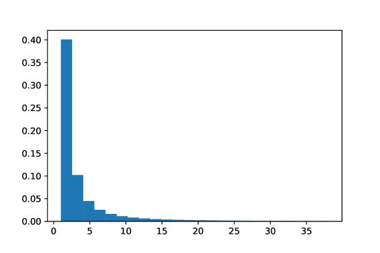
Figure 6: Monte Carlo results comparing the ratio of the actual path length seen by a pixel to the approximation $L=Dsin\theta$.

The next assumption involved the presentation of results by approximating $v_{x}=250\,$km s^-1. In fact, as discussed in the introduction, we expect that dark matter macros will have a Maxwellian velocity distribution as described by (1.2). Furthermore, we expect this distribution to be somewhat modified due to the Earths motion; specifically the Earth is moving around the Sun at $\sim 30\,$km s^-1 and that the Sun (and hence the Solar System) is moving around the center of the Milky Way at $\sim 220\,$km s^-1. As a result, we expect that there should be no significant contribution to the distribution for $v_{x}\lesssim 170\,$km s^-1. To determine the impact of these effects on the velocity distribution as detected at the Earth, we convolve of the macro Maxwellian distribution and the Earth’s speed distribution. This yields a velocity distribution where the majority of dark matter macros should have a velocity range between $170$ km s^-1 and $350$ km s^-1.

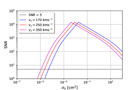
Figure 7: The SNR vs $\sigma_{x}$ for $D=10\,$km and varying $v_{x}$

Figures 3, 4 and 5 were generated assuming $v_{x}=250\,$km s^-1. In Figure 7 we reproduce Figure 4 with a fixed $D=10\,$km, but varying $v_{x}$. Here we see that the results presented in the preceding sections are a reliable measure for a wide range of realistic $v_{x}$ values. Only for small values of $v_{x}$, which make up a small fraction of the trajectories would there be significant deviation from the graphical results presented before this.

If a macro were to be detected, $v_{x}$ would be inferred from the motion of the macro and this would then be used to constrain the range of $\sigma_{x}$.

We have also taken into account the effects of attenuation of the signal as the photons propagate from the point of production to the detector. However, these effects have do not have a major impact on the our results. Attenuation due to Rayleigh scattering is easily calculated as a function of viewing angle and distance and corresponds to a maximum attenuation of about 70% of signal at the edge of our 20 km distance maximum fiducial distance for the FD detectors of Auger [25]. A typical value of Rayleigh attenuation corresponding to 0.5 is quite conservative and applied for both Auger and JEM-EUSO. Mie scattering due to ground-hugging aerosols can also contribute to attenuation. Atmospheric monitoring data taken over nine years of data using the Auger Central Laser Facility (CLF) show a typical aerosol optical depth is 0.04 even out to a vertical equivalent atmosphere of 10 km [26]. For Auger at 20 km this corresponds to an additional attenuation of $\left[1-\exp^{-0.04*\left(\frac{20}{10}\right)}\right]=$ 8%. Even on rare nights when the scattering optical depth exceeds 0.1, additional attenuation will not exceed 20 percent of our signal. The effect of aerosol scattering is even less prominent for JEM-EUSO which is viewing showers at a near-vertical angle from space.

6 Conclusion

Macroscopic dark matter is a broad class of alternatives to particulate dark matter that, compellingly, includes plausible Standard Model candidates. The passage of a macro through Earth’s atmosphere will cause dissociation and ionization of air molecules, resulting, through recombination, in a signal visible to Fluorescence Detectors such as those used to search for Ultra High Energy Cosmic Rays. As for such UHECR, large effective target areas are necessary to compensate for the low maximum flux of macros. Unlike UHECR, macros would be expected to travel several times faster than typical solar system objects, such as meteoroids, but still very non-relativistically. Existing and planned cosmic ray detectors would therefore need to make software, or possibly hardware, accommodations in order to detect the more slowly traced-out trajectories of macros. If they do, they have significant discovery potential for macroscopic dark matter of nuclear or greater density, including the most compelling non-black-hole candidates, able to probe up to masses of several tonnes, compared to current lower limits of just several tens of grams.

Emission		Pierre Auger Observatory
Mode		with $\tau_{bin}=100\mu s$
		Cross-Section (cm2)	Sensitivity
FS	Free-Streaming	$10^{-6}\leq\sigma_{x}\leq 10^{-5}$	Good
	(optically thin)		SNR $\geq 5$
			$10^{-2}\lesssim M_{x}\lesssim 10^{4}$ g
FSUT	Free-Streaming	$10^{-5}\leq\sigma_{x}\leq 10^{-2}$	Strong
	Unsaturated		SNR $>>5$
	$\tau_{bin}\leq t_{I0}$		$10^{-2}\lesssim M_{x}\lesssim 10^{4}$ g
FSST	Free-Streaming	$10^{-2}\leq\sigma_{x}\leq 10^{1}$	Strong
	Saturated		SNR $>>5$
	$\tau_{bin}\leq t_{I0}$		$1\lesssim M_{x}\lesssim 10^{4}$ g

Table 1: Tabular summary of sensitivity for Auger for different emission mechanisms assumed over a range of cross-section values. Rows correspond to ranges of cross-section and SNR calculations as delineated in Equations (4.3), (4.7a), (4.7b), and (4.7c).

Emission		JEM-EUSO
Mode		with $\tau_{bin}=2.5ms$
		Cross-Section (cm2)	Sensitivity
FS	Free-Streaming	$10^{-6}\leq\sigma_{x}\leq 10^{-5}$	Good
	(optically thin)		SNR $\sim$ 5
			$M_{x}\leq 10^{6}$ g
FSUT	Free-Streaming	$10^{-5}\leq\sigma_{x}\leq 10^{-2}$	Good
	Unsaturated		SNR $\geq 5$
	$\tau_{bin}\leq t_{I0}$		$M_{x}\lesssim 10^{7}$ g
FSST	Free-Streaming	$10^{-2}\leq\sigma_{x}\leq 10^{2}$	Strong
	Saturated		SNR $>>5$
	$\tau_{bin}\leq t_{I0}$		$M_{x}\lesssim 10^{7}$ g

Table 2: Tabular summary of sensitivity for JEM-EUSO for different emission mechanisms assumed over a range of cross-section values. Rows correspond to ranges of cross-section and SNR calculations as delineated in Equations (4.10), (4.11a), (4.11b), (4.11c), and (4.11d).

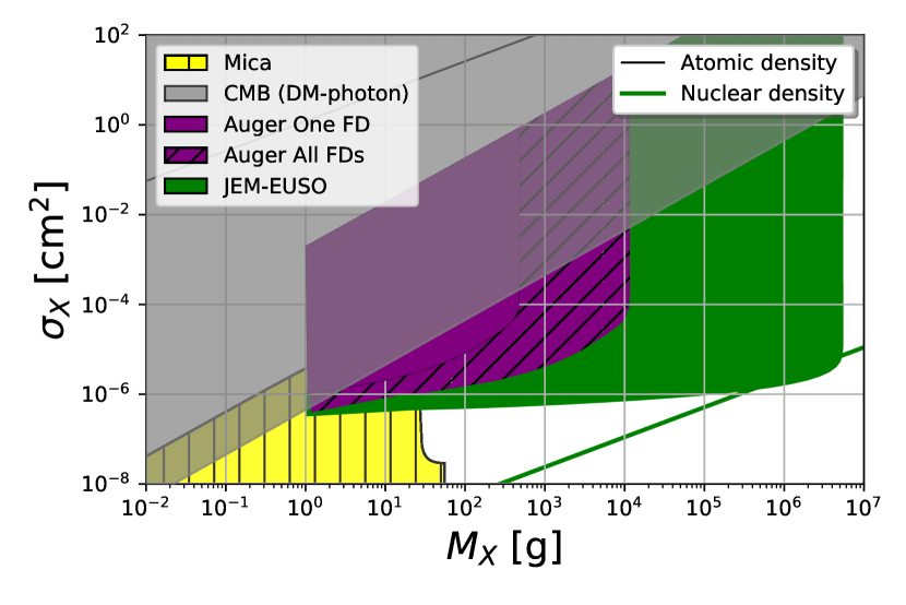
Figure 8: Figure 3 of [7] with the various regions of parameter space that could be probed by both PA(for one FD telescope in purple and the full array in purple with diagonal lines) and JEM-EUSO (in green).

References

- [1] Lelli, Federico and McGaugh, Stacy S. and Schombert, James M, SPARC: Mass Models for 175 Disk Galaxies with Spitzer Photometry and Accurate Rotation Curves,, arxiv:1606.09251
- [2] Witten E, Cosmic Separation of Phases,, Phys. Rev. D 30:272-285 (1984)
- [3] Bryan W. Lynn and Ann E. Nelson and Nikolaos Tetradis, Strange Baryon Matter, Nuc. Phys. B 345:186-209 (1990)
- [4] Ariel R. Zhitnitsky, ”Nonbaryonic” Dark Matter as Baryonic Color Superconductor, JCAP arxiv:hep-ph/0202161
- [5] David M. Jacobs and Glenn D. Starkman and Bryan W. Lynn, Macro Dark Matter, MNRAS 450:3418–3430 (2015) arxiv:1410.2236
- [6] David M. Jacobs and Glenn D. Starkman and Amanda Weltman, Resonant bar detector constraints on macro dark matter, Phys. Rev. D 91:115023 (2015) arxiv:1504.02779
- [7] David Cyncynates and Joshua Chiel and Jagjit Sidhu and Glenn D. Starkman, Reconsidering seismological constraints on the available parameter space of macroscopic dark matter, Phys. Rev. D 95:063006 (2017) arxiv:1610.09680
- [8] Capitelli, M and Colonna, G and Gorse, C and D’Angola, A Transport properties of high temperature air in local thermodynamic equilibrium, Euro. Phys. Jour. D 11:279-289 2000
- [9] Eisazadeh-Far, Kian and Metghalchi, Hameed and Keck, James C. Thermodynamic Properties of Ionized Gases at High Temperatures Jour. of Ener. Res. Tech. 133:022201 2011
- [10] Armstrong, B H and Johnston, R R and Kelly, P S, Opacity of High Temperature Air Lockheed Missiles And Space Company 1965
- [11] A. Bourdon and P. Vervisch, Three-body recombination rate of atomic nitrogen in low-pressure plasma flows, American Physical Society, 54:1888-1898 1996
- [12] A. Kramida and Yu. Ralchenko and J. Reader and NIST ASD Team, NIST Atomic Spectra Database (ver. 5.3) , [Online]. Available: http://physics.nist.gov/asd [2017, July 21]. National Institute of Standards and Technology, Gaithersburg, MD., 2015
- [13] The Pierre Auger Collaboration, The Pierre Auger Observatory, Nucl. Instrum. Meth. A 798:172-213 (2015) arxiv:1502.01323
- [14] The Pierre Auger Collaboration, The Pierre Auger Observatory Upgrade - Preliminary Design Report, (2016) arxiv:1604.03637
- [15] Argiro, Stefano Performance of the Pierre Auger Fluorescence Detector and Analysis of Well Reconstructed Events, Universal Academy Press, Inc p. 457-460 (2003)
- [16] Hermann-Josef, T The HEAT Telescopes of the Pierre Auger Observatory Status and First Data, 32nd International Cosmic Ray Conference Beijing 2011
- [17] R. Caruso and A. Insolia and S. Petrera and P. Privitera and F. Salamida and V. Verzi Measurement of the Sky Photon Background Flux at the Auger Observatory, 29th International Cosmic Ray Conference Pune 2005
- [18] The Pierre Auger Collaboration, The Fluorescence Detector of the Pierre Auger Collaboration, Nucl. Instrum. Meth. A 620:227-251 2010 arxiv:0907.4282
- [19] Y. Takahashi and JEM-EUSO Collaboration The Jem-Euso Mission, New J. Phys 11:065009 (2009) arxiv:0910.4187
- [20] A. Haungs and JEM-EUSO Collaboration Physics Goals and Status of JEM-EUSO and its Test Experiments, J. Phys.: Conf. Ser. 632:012092 (2015) arxiv:1504.02593
- [21] JEM-EUSO Collaboration JEM-EUSO Observational Technique and Exposure, SpringerLink 40:117-134 (2015)
- [22] O. Catalano et al. The atmospheric nightglow in the 300-400 nm wavelength: Results by the balloon-borne experiment Nuclear Instruments and Methods in Physics Research Section A: Accelerators, Spectrometers, Detectors and Associated Equipment, 480:547–554 (2002)
- [23] Marco Ricci and JEM-EUSO Collaboration The JEM-EUSO Program, J. Phys.: Conf. Ser. 718:052034 (2016)
- [24] H. Prieto-Alfonso and L. del Peral and M. Casolino and K. Tsuno and T. Ebisuzaki and M. D. Rodríguez Frías and JEM-EUSO Collaboration Multi Anode Photomultiplier Tube Reliability Assessment for the JEM-EUSO Space Mission, Reliability Engineering and System Safety 133:137-145 (2015)
- [25] The Pierre Auger Collaboration, The Piere Auger Observatory, Nucl. Instrum. Meth. A 798:172-213 2015 arxiv:1502.01323 (2015)
- [26] V. Laura for the Pierre Auger Collaboration, Atmospheric Aerosol Attenuation Measurements at the Pierre Auger Observatory, International Workshop on Atmospheric Monitoring for High-Energy Astroparticle Detectors (AtmoHEAD 2013) Gif-sur-Yvette, France, June 10-12, 2013, arxiv:1402.6186 (2014)