PACO: Global Signal Restoration via PAtch COnsensus

Abstract

Many signal processing algorithms break the target signal into overlapping segments (also called windows, or patches), process them separately, and then stitch them back into place to produce a unified output. At the overlaps, the final value of those samples that are estimated more than once needs to be decided in some way. Averaging, the simplest approach, often leads to unsatisfactory results. Significant work has been devoted to this issue in recent years. Several works explore the idea of a weighted average of the overlapped patches and/or pixels; others promote agreement (consensus) between the patches at their intersections. Agreement can be either encouraged or imposed as a hard constraint. This work develops on the latter case. The result is a variational signal processing framework, named PACO, which features a number of appealing theoretical and practical properties. The PACO framework consists of a variational formulation that fits a wide variety of problems, and a general admm-based algorithm for minimizing the resulting energies. As a byproduct, we show that the consensus step of the algorithm, which is the main bottleneck of similar methods, can be solved efficiently and easily for any arbitrary patch decomposition scheme. We demonstrate the flexibility and power of PACO on three different problems: image inpainting (which we have already covered in previous works), image denoising, and contrast enhancement, using different cost functions including Laplacian and Gaussian Mixture Models.

Key words. patch-based methods, global-local methods, patch consensus, inpainting, denoising, contrast enhancement.

AMS subject classifications. 49M30, 49M37, 65K05, 65K10, 90C25, 90C30.

1 Introduction

We refer to patch restoration methods to a family of techniques where the target signal is first broken down into smaller, possibly overlapping patches of some size and shape, some restoration method is applied to each patch separately, and the restored patches are stitched back together into their corresponding place to produce the complete restored signal (sometimes referred to as the global signal). This is a common technique, with many examples in audio (e.g. [26, 28, 35, 43]) and image processing (see e.g., [11, 16, 38, 39, 40, 41, 48]). A recent review on patch-based restoration methods for image processing can be found in [3]. Note that we are not considering methods such as [9, 45] (and their many variants) which estimate each sample separately using the surrounding patches as context, but only those that process the whole patch as a sub-signal.

When overlapping occurs, the final value of those samples that are estimated more than once must be resolved in some way. A traditional approach in audio processing methods is to apply a windowing function to the patches (e.g. Hanning); this procedure is backed by theoretical results related to the violation of frequency-based hypothesis during processing, but is widely applied to other methods as well. On the other hand, many recent, very successful patch-based methods do away with the overlapping issue by simply averaging the overlapped patches. This may incidentally help in covering up artifacts in the restoration process, but more often will simply smooth out the resulting global estimate (see e.g.[16]). To overcome such limitations via better stitching strategies has been the subject of several works over the last decade: some of them [13, 29, 33, 59, 61] are based on assigning weights to the different patches when averaging; others such as  [4, 20] assign a different weight to each pixel. We refer to these as weighted averaging methods.

An alternative to weighted averaging, which sidesteps the arbitrariness of defining appropriate weights, is to promote solutions where patches coincide at their intersection. This idea appears under the keyword patch disagreement in [57]; there, an iterative method is used to give more weight to the discrepancies between the estimated patches, with the aim of reducing such disagreement in the long run.

The problem of patch aggregation has also be studied from a probabilistic viewpoint in works such as [66] and [58]. The work  [66] is based on the observation that, after stitching, the averaged patches may no longer follow the prior from which they were modeled. The authors of [66] seek a remedy to this by augmenting the energy to be minimized with a quadratic term that penalizes the disagreement between the patches before and after stitching.

In [58], instead of directly averaging the patch estimates, the authors produce a unique probability model over the whole image by “stitching” the probability models of each independent patch via a well-defined fusion mechanism. Besides its own value as an original and powerful concept, the authors of [58] derive a new interpretation on the aforementioned work [66] as a particular fusion mechanism.

Back to the problem of averaging patch estimations, it was observed in  [22] that the agreement imposed in [66] would become a consensus constraint on the patches as the quadratic penalty coefficient grew to infinity. They then draw on this idea to propose a general consensus-based map denoising algorithm and a general admm-based method for solving it. In this sense, the method proposed in [22] can be seen as a particular case of our proposed framework. Furthermore, the work [22] analyzes the computational cost and bottlenecks of their proposed admm method to some degree. However, they fall short of fully exploiting the structure of the problem, leading to an overly conservative upper bound on the overall computational cost of the method. As we show below, this cost can be significantly reduced.

1.1 Contributions

This work proposes a general variational formulation for patch-based restoration methods, under a strict patch consensus constraint which can be applied to a wide family of problems, linear and non-linear, convex and non-convex, sparse or dense, to signals of any dimension. Below we summarize the contributions of our work.

Patch Consensus Framework

We provide a formal characterization of the Patch Consensus set, its geometrical properties, and its relationship with the space of signals. We then develop a general formulation for patch restoration problems under the paco constraint which can be applied to any method that can be written as the minimization of a cost function of the estimated patches and/or signal; this can be seen as a generalization of the one proposed in [22].

Optimization

We propose a method for solving the aforementioned family of problems based on a splitting strategy and the standard admm [15] algorithm. While our algorithm bears strong similarities to that proposed in [22], the latter is limited to the denoising case. Also, by retaining the patch extraction and stitching operations in matrix form, it does not fully exploit the geometry of the patch consensus space, which leads to a significantly higher computational cost.

In contrast, our admm-based algorithm can be readily applied to any variational patch-based restoration method. We also develop the special case of orthogonal linear patch models, and a Linearized admm algorithm (a.k.a. Uzawa’s Method [18]) for non-orthogonal linear patch models, which has the same convergence guarantees as admm while being computationally feasible even for very large signals. Both methods require significantly less computational resources than previously-proposed patch-consensus algorithms, and inherit the convergence properties of the admm method.

Stitching trick

As described earlier, the bottleneck of methods such as [66, 22, 5] lies in the “patch agreement step”, which might not be practical even for small problem sizes. In this work we show that the projection operator onto the consensus constraint set boils down to a simple composition of the patch stitching and extraction operations. This not only avoids the computation and/or storage of projection matrices, but is also very easy to implement, and generalizes to any arbitrary patch decomposition scheme including irregular grids, different patch sizes, etc., on signals of any dimension.

Global constraints

As mentioned above, the paco constraint guarantees a one-to-one correspondence between patch space (sometimes called “local” space) and global signal space; this allows formulations where arbitrary constraints are imposed on the global signal rather than on the patches. This is a crucial advantage of imposing strict consensus rather than promoting it in a lax way; we show this feature in the missing samples estimation method described section 4. Furthermore, for the types of patch extraction operations used in typical patch-based applications, the mapping between signal space and patch space can be considered to be an isometry. This allows for orthogonal projections on constraint sets to be performed on either space.

Applications and variants

We show the broad applicability and the potential of paco on three very different settings: inpainting, denoising, and contrast enhancement. Each problem is discussed in a self-contained section where we provide a brief introduction to the problem and derive the corresponding optimization algorithms. Note that the inpainting problem has already been covered in detail in [54, 55]; we repeat the main results here for completeness.

In order to further demonstrate the flexibility of the framework, different patch priors are explored in each case: we use Laplacian prior on dct coefficients for inpainting, and a Gaussian Mixture Model [65] for denoising. The dct-based inpainting case has already been covered in detail in [54] and [55]. For the other settings we provide preliminary results; a complete treatment of these methods, as well as experiments using other priors, will be published elsewhere.

1.2 Organization

The rest of the document is laid out as follows. We begin with an introduction to the general problem of patch-based signal processing in section 2. Section 3 provides a formal definition of the paco family of problems, as well as a general solution of the problem which serves as a basis for all the algorithms developed later. The next three sections provide self-contained treatments of different signal processing problems using paco: our previous work on inpainting is revisited in section 4, section 5 deals with denoising, and section 6 introduces paco for contrast enhancement. We conclude our treatment in section 7.

2 Patch-based methods

The methods that we are interested in this paper involve three stages that may be repeated until some convergence criterion is met: patch extraction, patch estimation, and patch stitching. Recall that we are interested in methods that estimate whole patches rather than a single pixel (e.g., the center) such as in [9]. We will now illustrate these concepts on a simple one-dimensional case.

2.1 Patch extraction

Figure 1: Patch extraction operator $\mathbf{{Y}}=\mathcal{R}(\mathbf{{x}})$ for a signal $\mathbf{{x}}$ of length $N=6$ and patches of size $m=3$; patches are arranged as columns on an $m{\times}n$ matrix $\mathbf{{Y}}$ where the column $\mathbf{{y}}_{k}$ contains the patch starting at offset $k$ in $\mathbf{{x}}$.

Figure 2: Average patch stitching operator $\hat{\mathbf{{x}}}=\mathcal{S}(\hat{\mathbf{{Y}}})$. Each sample $\hat{x}_{j}$ is the average of all its estimates in $\hat{\mathbf{{Y}}}$. In our example, this corresponds to the average of each anti-diagonal of $\hat{\mathbf{{Y}}}$.

Given a 1D signal $\mathbf{{x}}=(x_{1},\ldots,x_{N})\in\mathbb{X}=\mathbb{R}^{N}$ of length $N$, the patch extraction is a linear operator $\mathcal{R}$ determined by a patch extraction matrix $\mathbf{{R}}^{\intercal}=[\;\mathbf{{R}}_{1}^{\intercal}\;|\;\mathbf{{R}}_{2}^{\intercal}\;|\;\cdots\;|\;\mathbf{{R}}_{n}^{\intercal}\;],$ where each sub-matrix $\mathbf{{R}}_{j},j=1,\ldots,n$ copies (extracts) samples from $\mathbf{{x}}$ into a sub-vector $\mathbf{{y}}_{j}$, which we call a patch. Which samples, how many samples, and how many copies of each sample in $\mathbf{{x}}$ are extracted onto $\mathbf{{y}}_{j}$ is arbitrary and may depend on $j$, so that the dimension of each patch is some $m_{j}\in\mathbb{N}$. The result of the extraction operator is a patches vector $\mathbf{{y}}^{\intercal}=[\mathbf{{y}}_{1}^{\intercal}\;|\;\mathbf{{y}}_{2}^{\intercal}\;|\;\ldots\;|\;\mathbf{{y}}_{n}^{\intercal}]\in\mathbb{R}^{\sum_{j=1}^{n}{m_{j}}}$. The space $\mathbb{Y}=\mathbb{R}^{\sum_{j=1}^{n}{m_{j}}}$ is called the patches space. In the common case where $m_{j}=m$ for all $j$, it may be convenient to rearrange the patches vector $\mathbf{{y}}\in\mathbb{R}^{mn}$ as a matrix $\mathbf{{Y}}\in\mathbb{R}^{m\times{n}}$, where the patches $\mathbf{{y}}_{j}$ are arranged as columns; many formulations are presented in this way hereafter. Formally, however, we will always refer to the extracted patches as a vector belonging to the patch space $\mathbb{Y}$.

In the example of Figure 1 we have a 1D signal of length $N=6$, patches of size $m=3$ and $\mathbf{{R}}_{j}=\left[\mathbf{{e}}^{j}\;|\;\mathbf{{e}}^{j+1}|\mathbf{{e}}^{j+2}\right]$ $j=1,2,3,4$. More generally, we will have $\mathbf{{R}}_{j}^{\intercal}=\left[\mathbf{{e}}^{1}\;|\;\mathbf{{e}}^{1+s}\;|\;\mathbf{{e}}^{1+2s}\;|\;\ldots\;\right]$ where $s>1$ is called the stride, that is, the separation in space between one patch an its neighbor. The case $s=1$ depicted in Figure 1 yields fully overlapped patches; the extreme case $s=3$ yields non-overlapping patches. The preceding discussion generalizes to signals $\mathbf{{x}}$ of any dimension by vectorizing $\mathbf{{x}}$ prior to extraction: $\mathbf{{y}}_{j}=\mathbf{{R}}_{j}\mathrm{vec}(\mathbf{{x}})$. Here $\mathrm{vec}(\cdot)$ arranges its argument into a vector by traversing its elements in some predefined order. In our case, for $2D$ signals of size $M{\times}N$, we follow a row-major ordering, that is, the output vector is the concatenation of the $M$ input rows. The inverse of $\mathrm{vec}(\cdot)$ is called the matrification operator and is denoted by $\mathrm{mat}(\cdot)$.

Geometry of the problem

The operator $\mathcal{R}$ is linear and injective. Thus, its image $\mathbb{C}$ is a subspace of the patches space $\mathbb{Y}$. If $\mathcal{R}$ extracts all the samples from $\mathbf{{x}}$ then it also defines a linear bijection between $\mathbb{X}$ and $\mathbb{C}$. As defined, the elements of $\mathbb{C}$ which are mapped from the same sample in $\mathbf{{x}}$ are all equal; for reasons that will become clear soon, we say that these elements are in consensus. Thus we call $\mathbb{C}$ the consensus set.

The sets $\mathbb{X}$ and $\mathbb{C}$ are, however, not isometric. It is easy to verify that this can only happen if $\mathbb{C}$ contains exactly the same number of copies of each sample in $\mathbb{X}$. Most common patch extraction schemes used in the literature do not comply with this, as samples in the borders usually belong to fewer patches than those in the center. However, for most signals and, in particular images, of practical interest, the border samples are few and thus the mappings $\mathbb{X}$ and $\mathbb{C}$ can be considered isometric for most practical purposes. This will prove important, as it allows to perform orthogonal projections onto convex sets defined in $\mathbb{C}$ in the (usually much smaller) space $\mathbb{X}$.

2.2 Patch averaging and the stitching trick

In a signal restoration setting one does not observe the true or clean signal $\tilde{\mathbf{{x}}}$, but a distorted version $\mathbf{{x}}$ (which usually has the same size and dynamic range as $\tilde{\mathbf{{x}}}$), and the task is to infer $\tilde{\mathbf{{x}}}$ from $\mathbf{{x}}$. We denote the result of this inference as $\hat{\mathbf{{x}}}$, and call it the restored or estimated signal indistinctly. The patches vector extracted from $\mathbf{{x}}$ is correspondingly denoted by $\mathbf{{y}}$. The idea is to estimate the signal $\tilde{\mathbf{{x}}}$ by recomposing it from an estimate $\hat{\mathbf{{y}}}$, which is itself a function of $\mathbf{{y}}$. In general, however, $\mathbf{{y}}\notin\mathbb{C}$.

By stitching we refer to the operation that maps a patches vector $\hat{\mathbf{{y}}}\in\mathbb{Y}$ onto an estimated signal $\hat{\mathbf{{x}}}$. In general, this operator is not unique. A common choice is to seek for the signal estimate $\hat{\mathbf{{x}}}$ whose patches, when extracted, are as close as possible to the individually estimated ones in $\hat{\mathbf{{y}}}$. If we measure this distance using $\ell_{2}$ norm, we obtain the classical least squares estimator:

$$\hat{\mathbf{{x}}}_{ls}=\arg\min_{\mathbf{{x}}}\|\mathbf{{R}}\mathbf{{x}}-\hat{\mathbf{{y}}}\|_{2}=\left(\sum_{j}\mathbf{{R}}_{j}^{\intercal}\mathbf{{R}}_{j}\right)^{-1}\sum_{j}\mathbf{{R}}_{j}^{\intercal}\hat{\mathbf{{y}}}_{j}=(\mathbf{{R}}^{\intercal}\mathbf{{R}})^{-1}\mathbf{{R}}^{\intercal}\hat{\mathbf{{y}}}.$$ (1)

Equation 1 is interpreted as follows: it is easy to verify that $\mathbf{{R}}_{j}^{\intercal}\hat{\mathbf{{y}}}_{j}$ puts back the patch $\hat{\mathbf{{y}}}_{j}$ in its corresponding place in $\hat{\mathbf{{x}}}$; thus, $\mathbf{{R}}^{\intercal}\hat{\mathbf{{y}}}$ produces a vector of length $N$ where the $i$-th element contains the sum of all the elements of $\hat{\mathbf{{y}}}$ that are mapped there by one or more $\mathbf{{R}}_{j}$. On the other hand $\mathbf{{R}}_{j}^{\intercal}{\mathbf{{R}}_{j}}$ is a diagonal matrix with $m$ ones, and so $\mathbf{{R}}^{\intercal}\mathbf{{R}}=\sum_{j}\mathbf{{R}}_{j}^{\intercal}{\mathbf{{R}}_{j}}$ is a diagonal matrix whose $(i,i)$-th element counts how many $\mathbf{{R}}_{j}$s have mapped some element of $\hat{\mathbf{{y}}}$ to the sample $i$. Thus, the $i$-th entry of the right hand side of Eq. 1 is the average of all the different estimates of the $i$-th sample in $\hat{\mathbf{{y}}}$. We call the operator defined in Eq. 1 as the average stitching operator and denote it by $\mathcal{S}:\mathbb{Y}\rightarrow\mathbb{R}^{N}$, $\hat{\mathbf{{x}}}=\mathcal{S}(\hat{\mathbf{{y}}})$. The extraction operator $\mathcal{R}$ is given by $\mathbf{{y}}=\mathcal{R}(\mathbf{{x}})=\mathbf{{R}}\mathbf{{x}}$. If we compose this with the stitching operator $\mathcal{S}$ defined earlier we obtain

$$\mathcal{R}[\mathcal{S}(\hat{\mathbf{{y}}})]=\mathbf{{R}}(\mathbf{{R}}^{\intercal}\mathbf{{R}})^{-1}\mathbf{{R}}^{\intercal}\hat{\mathbf{{y}}}=\mathrm{\Pi}_{\mathbb{C}}(\hat{\mathbf{{y}}}),$$ (2)

where $\mathrm{\Pi}_{\mathbb{C}}(\hat{\mathbf{{y}}})$ is the orthogonal projection of $\hat{\mathbf{{y}}}\in\mathbb{Y}$ onto $\mathbb{C}$. Thus, we conclude that the projector operator Eq. 2 from $\mathbb{Y}$ onto $\mathbb{C}$ can be written as the composition of the extraction operator with its corresponding average stitching operator. Although Eq. 2 is a well known result, to the best of our knowledge, its straightforward implementation as the aforementioned composition has not been fully exploited in the literature; this is why we call it a trick. Rather, works such as [5, 22] compute the orthogonal projection matrix $\mathbf{{R}}(\mathbf{{R}}^{\intercal}\mathbf{{R}})^{-1}\mathbf{{R}}^{\intercal}$ explicitly, something that quickly becomes unwieldy as the signal size increases even if the structure of such matrix is exploited (e.g., block sparsity). This is further complicated if, instead of the patches, the stitching is written in terms of some affine transformation of the patches such as $\mathbf{{y}}_{j}=\mathbf{{D}}\mathbf{{a}}_{j}+b$, such as in [5, 22]. The stitching trick will only work directly on patches, or some orthogonal transformation of them. Later we will see how to deal with the affine case. What is also remarkable is that the procedure does works for any arbitrary extraction operator $\mathcal{R}$. In particular, it does not require patches to be of the same shape and/or number of samples.

3 PACO: The PAtch COnsensus problem

3.1 General consensus problems

This subsection is based on the monograph [49, Chapter 5].

In the context of parallel and distributed optimization, a common problem is to minimize a function $f(\zeta)=\sum_{j=1}^{r}f_{j}(\zeta)$, where $f_{j}(\zeta)$ are functions that can only be evaluated locally, say at some node $j$ on a spatially distributed network with $r$ nodes, but which all depend on the same global variable $\zeta\in\mathbb{R}^{m}$. One strategy to solve this problem in a decentralized way is for each node to have its own local copy of $\zeta$, $\zeta^{j}$, which it then optimizes in terms of its local function $f_{(}\zeta^{j})$. In the end, however, we want all the $\zeta^{j}$ to be equal. For this we define the consensus set as $\mathbb{G}=\left\{(\zeta^{1},\zeta^{2},\ldots,\zeta^{r})\in\mathbb{R}^{m{\times}r}:\zeta^{1}=\zeta^{2}=\ldots=\zeta^{r}\right\}$ and constrain the final solution to fall within $\mathbb{G}$. This gives rise to the following global consensus problem:

$$\min_{(\zeta^{1},\zeta^{2},\ldots,\zeta^{r})\in\mathbb{G}}\sum_{j=1}^{r}f_{j}(\zeta^{j}).$$

Clearly, $\mathbb{G}$ is a linear subspace of $\mathbb{R}^{m{\times}r}$ (e.g., the line $x=y$ in $\mathbb{R}^{2}$). Let $\mathrm{\Pi}_{\mathbb{G}}(\cdot)$ denote the orthogonal projection operator from $\mathbb{R}^{m{\times}r}$ onto $\mathbb{G}$. It is straightforward to verify that,

$$\mathrm{\Pi}_{\mathbb{G}}{(\zeta^{1},\zeta^{2},\ldots,\zeta^{r})}=(\bar{\zeta},\bar{\zeta},\ldots,\bar{\zeta}),\quad\bar{\zeta}=\frac{1}{r}\sum_{j}\zeta^{j}.$$

Let $[m]$ be a shorthand for the set $\{1,2,\ldots,\}$. Consider the more general case where each local copy $\zeta^{j}$ has an index subset $c_{j}\subseteq[m]$ associated to it, and consensus with any other copy $\zeta^{j^{\prime}}$ is required only for those entries indexed by $c_{j}\cap c_{j^{\prime}}$. The partial consensus set $\mathbb{G}^{\prime}$ is defined as follows:

$$\mathbb{G}^{\prime}=\left\{(\zeta^{1},\zeta^{2},\ldots,\zeta^{r}):\zeta^{j}_{i}=\zeta^{j^{\prime}}_{i},\forall\,i\in c_{j}\cap c_{j^{\prime}},\forall\,j,j^{\prime}\in[n],j\neq j^{\prime}\right\}.$$ (3)

The corresponding partial consensus problem is given by:

$$\min_{(\zeta^{1},\zeta^{2},\ldots,\zeta^{r})\in\mathbb{G}^{\prime}}\sum_{j=1}^{r}f_{j}(\zeta^{j}).$$ (4)

It is easy to show that the projection onto $\mathbb{G}^{\prime}$ is given by

$$\mathrm{\Pi}_{\mathbb{G}}(\zeta^{j}_{i})=\bar{\zeta}_{i}:\bar{\zeta}_{i}=\frac{\sum_{j:i\in c_{j}}\zeta^{j}_{i}}{\sum_{j:i\in c_{j}}1}.$$ (5)

In words, after projection, the $i$-th element of all vectors that include $i$ in their corresponding set $c_{j}$ will be the average of the values of the $i$-th elements on those vectors before projection.

3.2 Patch consensus problem

Given a patch extraction operator $\mathcal{R}:\mathbb{X}\rightarrow\mathbb{Y}$ with its corresponding consensus set $\mathbb{C}$, a cost function $f(\mathbf{{y}}):\mathbb{Y}\rightarrow\mathbb{R}$, and an optional constraint set $\Omega\subseteq\mathbb{Y}$, the paco problem is stated as follows:

$$\hat{\mathbf{{y}}}=\arg\min_{\mathbf{{z}}}f(\mathbf{{z}})\quad\mathrm{s.t.}\quad\mathbf{{z}}\in\Omega\cap\mathbb{C}.$$ (6)

We begin by showing that, when $\Omega=\mathbb{Y}$, Eq. 6 is a especial case of Eq. 5. We will treat the general case $\Omega\neq\mathbb{C}$ later. At this point, we shall remind the reader that $\mathbb{C}$ is isomorphic to $\mathbb{X}$, so that the constraint set $\Omega$ can be defined in either $\mathbb{X}$ or $\mathbb{C}$, or a combination of both. For example, in order to clip the estimated samples to the range $[0-255]$ we could define $\Omega=\{\mathbf{{z}}\in\mathbb{Y}:\mathcal{S}(\mathbf{{z}})\in[0,255]^{N}\}$.

Proposition 1.

The patch consensus set $\mathbb{C}$ is a particular case of the general consensus set $\mathbb{G}^{\prime}$ and so the paco problem is of the form Eq. 4.

Proof.

It suffices to define $\zeta_{j}=\mathbf{{R}}_{j}^{\intercal}\mathbf{{y}}_{j}$ and $c_{j}=\mathrm{nonzero}(\mathrm{diag}(\mathbf{{R}}_{j}^{\intercal}{\mathbf{{R}}_{j}}))$. Here $\mathrm{diag}(\cdot)$ returns the diagonal of an $N{\times}N$ square matrix as a vector of length $N$, and $\mathrm{nonzero}(\cdot)$ returns the indices of the nonzero elements in its argument. Note that, as defined, $c_{j}$ contains the indices of the samples filled in by $\mathbf{{y}}_{j}$. Thus, the requirement that $\mathbf{{y}}_{j}$ and $\mathbf{{y}}_{j^{\prime}}$ should coincide at $c_{j}\cap c_{j^{\prime}}$ matches the definition given before for the consensus set in Eq. 3 for this particular choice of $\zeta_{j}$ and $c_{j}$. Now, given $f(\mathbf{{y}})=\sum_{j}f_{j}(\mathbf{{y}}_{j})$ in Eq. 6, we define $f^{\prime}_{j}(\zeta_{j})=f_{j}(\mathbf{{R}}\zeta_{j})=f_{j}(\mathbf{{y}}_{j})$ and plug it into Eq. 4. ∎

Corollary 2.

The orthogonal projection onto the patch consensus set $\mathbb{C}$ is given by the stitching trick, $\mathrm{\Pi}_{\mathbb{C}}(\hat{\mathbf{{y}}})=\mathcal{R}[\mathcal{S}(\hat{\mathbf{{y}}})]$, as in Eq. 2.

Proof.

We have established that the patch consensus set $\mathbb{C}=\mathbb{G}^{\prime}$, and that Eq. 2 gives $\mathrm{\Pi}_{\mathbb{C}}(\hat{\mathbf{{y}}})$. Thus, $\mathrm{\Pi}_{\mathbb{C}}({\hat{\mathbf{{y}}}})=\mathrm{\Pi}_{\mathbb{C}}({\hat{\mathbf{{y}}}})=\mathcal{R}[\mathcal{S}(\hat{\mathbf{{y}}})]$. ∎

3.3 Optimization

We define the convex indicator function associated to the paco constraint set $\mathbb{C}\cap\Omega$, $g(\cdot):\mathbb{Y}\rightarrow\mathbb{R}\cup\{+\infty\}$,

$$g(\xi)=\left\{\begin{array}[]{lcl}0&,&\xi\in\mathbb{C}\cap\Omega\\ +\infty&,&\xi\notin\mathbb{C}\cap\Omega\end{array}\right.$$

This allows us to transform the paco problem into an unconstrained one,

$$\hat{\mathbf{{y}}}=\arg\min_{\xi}f(\xi)+g(\xi).$$ (7)

The problem Eq. 7 will be convex if the function $f(\cdot)$ and the set $\Omega$ are also convex. This allows for convex restoration problems to be defined under consensus constraints. This being said, the paco framework Eq. 7 is not limited to convex problems.

The following method is based on the proximal operator form [49] of the popular Alternating Directions Method of Multipliers (admm) [15]. The proximal operator of a function $f(\cdot)$ with parameter $\lambda$ is given by,

$$\mathrm{prox}_{\lambda f}\left(y\right):=\arg\min_{\xi}f(\xi)+\frac{1}{2\lambda}\|\xi-y\|^{2}.$$ (8)

The proximal operator has many interesting properties (see [49] and references therein). Among them, if $g(\cdot)$ is the indicator function of a set $A$ we have that

$$\mathrm{prox}_{\lambda g}\left(\cdot\right)=\mathrm{\Pi}_{A}(\cdot).$$

This is particularly useful within the paco framework, as $\mathrm{\Pi}_{\mathbb{C}}(\cdot)$ can be computed efficiently using the stitching trick described in subsection 2.1, Equation 2. However, in general, this trick cannot be applied directly to Eq. 7. In order to do that, we need to reformulate Eq. 7 so that projecting onto the constraint set, and minimizing the target cost function $f(\cdot)$, can be done separately. One such reformulation is the so called splitting,

$$(\hat{\mathbf{{y}}},\hat{\mathbf{{z}}})=\arg\min_{\xi,\zeta}f(\xi)+g(\zeta)+\frac{1}{2\lambda}\|\xi-\zeta\|_{2}^{2}\quad\mathrm{s.t.}\quad\xi=\zeta.$$ (9)

The admm provides a general way to obtain a solution to Eq. 9 which is guaranteed to be global if the problem is convex, and local otherwise. The particular admm steps for this case are described in Algorithm 1.

Algorithm 1 Generic ADMM program for solving PACO

0:  $\mathbf{{z}}^{(0)}\in\mathbb{Y}$

0:  $\lambda>0$

  $t\leftarrow 0$

  $\mathbf{{u}}^{(0)}\leftarrow\mathbf{0}$

  repeat

     $\mathbf{{y}}^{(t+1)}\leftarrow\mathrm{prox}_{\lambda f}\left(\mathbf{{z}}^{(t)}-\mathbf{{u}}^{(t)}\right)$ {problem dependent:$f$}

     $\mathbf{{z}}^{(t+1)}\leftarrow\Pi_{\mathbb{C}\cap\Omega}\left(\mathbf{{y}}^{(t+1)}+\mathbf{{u}}^{(t)}\right)$ {problem dependent:$\Omega$}

     $\mathbf{{u}}^{(t+1)}\leftarrow\mathbf{{u}}^{(t)}+\mathbf{{y}}^{(t+1)}-\mathbf{{z}}^{(t+1)}$

     $t\leftarrow t+1$

  until convergence

  return  $\hat{\mathbf{{y}}}\leftarrow\mathbf{{y}}^{(t)}$

  return  $\hat{\mathbf{{z}}}\leftarrow\mathbf{{z}}^{(t)}$

3.4 Applying PACO

paco is a variational method and thus can be fitted to any signal restoration problem that can be written in terms of a cost function and a constraint set. This includes the large family of probabilistic methods where $f(\mathbf{{y}}_{j})$ measures the likelihood of the patch $\mathbf{{y}}_{j}$, either a priori or a posteriori; a few relevant examples of this are [1, 53, 55, 58, 65, 66].

Another group of methods includes penalized likelihood methods where the penalties are not necessarily probabilistic. These include Total Variation [25] and general linear models based on orthogonal transforms, wavelets [12, 42], learned dictionaries [2, 17, 36] and sets of linear convolutional filters such as [8]. Some of these methods consider the energy in terms of the whole image. Still, these images could be seen as patches of a much larger image (for example, in a distributed application for processing huge images, such as those produced by modern scientific telescopes).

In [51, 52] the patches of the image, seen as points in patch space, are assumed to trace a smooth curve over a low-dimensional manifold. Estimations are then obtained by displacing those points so that the resulting curves are smooth. There is also a large body of works on image processing based on Partial Differential Equations (PDE) which are also variational in nature; see the book [10] for a complete review of the theory and applications of this approach. More recently, this idea has been combined within the framework of Non-Local methods; the inpainting methods that we use for comparison [4, 19, 46] all fall into this category.

Finally, other desired features of the patches can be expressed in terms of minimizing a cost function. Examples of this are [32, 47].

As per the constraint sets, these are usually avoided, as dealing with them usually (but not always) leads to slower convergence rates. Perhaps the most common ones are the $\ell_{2}$ ball constraint, used in some denoising formulations to keep the solutions close to the observed noisy signal, and the inpainting constraint (to be introduced later), which imposes that the results should coincide in those places where the input image is already known. The lack of hard constraints besides consensus is good news for paco, as it tends to complicate the projection stages. As mentioned, fortunately, this is not always the case, as some of our applications show.

In order to apply the paco framework to a particular restoration problem, the user needs to provide two ingredients: the proximal operator of the problem-dependent cost function $f(\cdot)$, and the projection operator onto $\Omega\cap\mathbb{C}$. If $\Omega=\mathbb{Y}$ then $g=\mathrm{\Pi}_{\mathbb{C}}(\cdot)$ can be efficiently obtained using stitching trick Eq. 2,

$$\mathbf{{z}}^{(t+1)}=\mathcal{R}\left[\mathcal{S}\left(\mathbf{{y}}^{(t+1)}+\mathbf{{u}}^{(t)}\right)\right].$$

If $\Omega\subset\mathbb{C}$ is affine, the solution can be obtained by iteratively projecting onto $\Omega$ and $\mathbb{C}$ until convergence (this method is sometimes referred to as POCS). If $\Omega\neq\mathbb{C}$ is convex but not affine, a general solution can be obtained using Dykstra’s algorithm, which we provide in Algorithm 2 for reference.

Algorithm 2 Dykstra’s algorithm for computing the projection of a point $\alpha$ onto the intersection of two sets $A$ and $B$

0:  point $\alpha$, sets $A$ and $B$

  $t\leftarrow 0$, $\alpha^{(0)}\leftarrow\alpha$

  $\mathbf{{p}}^{(0)}\leftarrow\mathbf{0}$, $\mathbf{{q}}^{(0)}\leftarrow\mathbf{0}$

  repeat

     $\beta^{(t)}\leftarrow\Pi_{B}(\alpha^{(t)}+\mathbf{{p}}^{(t)})$

     $\mathbf{{p}}^{(t+1)}\leftarrow\alpha^{(t)}+\mathbf{{p}}^{(t)}-\beta^{(t)}$

     $\alpha^{(t+1)}\leftarrow\Pi_{A}(\beta^{(t)}+\mathbf{{q}}^{(t)})$

     $\mathbf{{q}}^{(t+1)}\leftarrow\beta^{(t)}+\mathbf{{q}}^{(t)}-\alpha^{(t+1)}$

     $t\leftarrow t+1$

  until convergence

  return  $\alpha^{(t)}$

3.5 Particular case: linear patch models

Note that, starting in this section, we well switch to the patch matrix notation defined in section 1, where patches are arranged as columns of a matrix $\mathbf{{Y}}$. The same goes to the corresponding coefficient vectors, and all auxiliary variables.

In many patch-based algorithms, patches are modeled in terms of some linear transformation, i.e., $\mathbf{{Y}}=\mathbf{{D}}\mathbf{{Y}}$, where $\mathbf{{D}}$ is some matrix, and the cost function is a prior defined over the coefficients matrix $\mathbf{{A}}$. Typical cases include the fft or dct, and some wavelet transforms. The corresponding splitting formulation is given in terms of the coefficients matrix $\mathbf{{A}}$ and its split variable $\mathbf{{B}}$:

$$(\hat{\mathbf{{A}}},\hat{\mathbf{{Z}}})=\arg\min_{\mathbf{{A}},\mathbf{{B}}}f(\mathbf{{A}})+g(\mathbf{{D}}\mathbf{{B}})+\frac{1}{2\lambda}\|\mathbf{{A}}-\mathbf{{B}}\|_{F}^{2}\quad\mathrm{s.t.}\quad\mathbf{{A}}=\mathbf{{B}},$$ (10)

Let $g^{\prime}(\mathbf{{B}})\stackrel{{\scriptstyle\Delta}}{{=}}g(\mathbf{{D}}\mathbf{{B}})$ . If $\mathbf{{D}}$ is orthogonal, it is easy to show that $\mathrm{prox}_{{\lambda}g^{\prime}}\left(\cdot\right)=\mathbf{{D}}^{-1}\mathrm{prox}_{{\lambda}g}\left(\mathbf{{D}}\cdot\right).$ This allows us to apply such patch models with only a minor modification to the general solution given in Algorithm 1. The paco-dct inpainting problem described in section 4 shows an example of exploiting the orthogonality of the dct type II.

Many recent patch-based algorithms consider the more general situation where $\mathbf{{D}}$ is non-orthogonal. A notable case is the use of sparse linear models defined in terms of over-complete dictionaries where $\mathbf{{D}}\in\mathbb{R}^{m{\times}p}$ with $p>m$. Imposing the consensus constraint directly on the dictionary coefficients $\mathbf{{a}}_{j}$ as has been proposed in previous works such as [66, 22, 5], leads to a projection operator which is unwieldy to work with even for very small signals and dictionaries. Referring back to Eq. 1, we have $\hat{\mathbf{{x}}}_{ls}=(\mathbf{{R}}^{\intercal}\mathbf{{R}})^{-1}\mathbf{{R}}^{\intercal}\mathrm{vec}(\mathbf{{D}}\hat{\mathbf{{A}}})$. Now, under the consensus constraint, we must have $\mathbf{{R}}_{j}\hat{\mathbf{{x}}}=\mathbf{{D}}\hat{\mathbf{{a}}}_{j}$ for all $j$ or, equivalently, $\mathbf{{R}}\hat{\mathbf{{x}}}=\mathrm{vec}(\mathbf{{D}}\hat{\mathbf{{A}}})$. Combined with Eq. 1 we obtain:

$$\mathrm{vec}(\mathbf{{D}}\hat{\mathbf{{A}}}) = \mathbf{{R}}(\mathbf{{R}}^{\intercal}\mathbf{{R}})^{-1}\mathbf{{R}}^{\intercal}\mathrm{vec}(\mathbf{{D}}\hat{\mathbf{{A}}})$$

$$(\mathbf{{R}}^{\intercal}\mathbf{{R}})\mathbf{{B}}\mathrm{vec}(\hat{\mathbf{{A}}}) = \mathbf{{R}}^{\intercal}\mathbf{{B}}\mathrm{vec}(\hat{\mathbf{{A}}})$$

$$\mathrm{vec}(\hat{\mathbf{{A}}}) = [(\mathbf{{R}}\mathbf{{B}})^{\intercal}\mathbf{{R}}\mathbf{{B}}]^{-1}(\mathbf{{R}}\mathbf{{B}})^{\intercal}\mathbf{{B}}\mathrm{vec}(\hat{\mathbf{{A}}})$$

$$\mathrm{vec}(\hat{\mathbf{{A}}}) = \mathbf{{P}}\mathrm{vec}(\hat{\mathbf{{A}}})$$

where $\mathbf{{B}}=(\mathbf{{I}}_{n{\times}n}\otimes\mathbf{{D}})$ and $\otimes$ is the kronecker product (see [7] for this result), and $\mathbf{{P}}=[(\mathbf{{R}}\mathbf{{B}})^{\intercal}\mathbf{{R}}\mathbf{{B}}]^{-1}(\mathbf{{R}}\mathbf{{B}})$ is a (non-orthogonal) projection matrix. The consensus set is given in terms of $\mathbf{{A}}$ as

$$\mathbb{C}_{\mathbf{{A}}}=\left\{\mathbf{{A}}:(\mathbf{{I}}-\mathbf{{P}})\mathbf{{A}}=0\right\},$$

so it is again a linear subspace of the signal coefficients space. However, by inspecting $\mathbf{{P}}$, it is also clear that this is a matrix whose size $mn{\times}mn$ can be extremely large for practical problems (e.g., $n=10^{6}$, $m=64$). Even considering the redundancy implied by the Kronecker product, and the sparsity of $\mathbf{{P}}$, the number of non-zero elements in $\mathbf{{P}}$ is typically very large, making it infeasible to compute $\mathrm{\Pi}(\mathbf{{A}})=\mathrm{vec}^{-1}(\mathbf{{P}}\mathrm{vec}(\mathbf{{A}}))$ directly.

The issue with the preceding strategy is to attempt to project the coefficients matrix $\mathbf{{A}}$ directly onto the consensus constraint. The solution presented here is based on the Linearized admm (ladmm) or Uzawa’s Method [18] for solving Eq. 6; this method constructs the augmented Lagrangian for the constraint $\mathbf{{Z}}=\mathbf{{D}}\mathbf{{A}}$ and then solves a linear approximation of it around $\mathbf{{Z}}$ in each iteration. Global convergence is guaranteed as long as its parameter $\mu$ satisfies $0<\mu\leq\lambda/\|\mathbf{{D}}\|_{2}^{2}$. The ladmm algorithm is given by,

$$\mathbf{{A}}^{(t+1)} \leftarrow \mathrm{prox}_{\mu f}\left[\mathbf{{A}}^{(t)}-(\mu/\lambda)\mathbf{{D}}^{\intercal}(\mathbf{{D}}\mathbf{{A}}^{(t)}-\mathbf{{Z}}^{(t)}+\mathbf{{U}}^{(t)})\right]$$

$$\mathbf{{Z}}^{(t+1)} \leftarrow \mathrm{prox}_{\lambda c}\left[\mathbf{{D}}\mathbf{{A}}^{(t+1)}+\mathbf{{U}}^{(t)}\right]$$

$$\mathbf{{U}}^{(t+1)} \leftarrow \mathbf{{U}}^{(t)}+\mathbf{{D}}\mathbf{{A}}^{(t+1)}-\mathbf{{Z}}^{(t+1)}.$$

The corresponding ladmm algorithm for paco is given by

$$\mathbf{{A}}^{(t+1)} \leftarrow \mathrm{prox}_{\lambda{f}}\left[\mathbf{{A}}^{(t)}-(\mu/\lambda)\mathbf{{D}}^{\intercal}({\hat{\mathbf{{Y}}}^{(t)}}-\mathbf{{Z}}^{(t)}+\mathbf{{U}}^{(t)}\right]$$

$$\hat{\mathbf{{Y}}}^{(t+1)} \leftarrow {\mathbf{{D}}\mathbf{{A}}^{(t+1)}}+\mathbf{{U}}^{(t)}$$

$$\mathbf{{Z}}^{(t+1)} \leftarrow {\mathcal{R}[\,\mathcal{S}(\hat{\mathbf{{Y}}})\,]}$$

$$\mathbf{{U}}^{(t+1)} \leftarrow \mathbf{{U}}^{(t)}+{\hat{\mathbf{{Y}}}^{(t+1)}}-\mathbf{{Z}}^{(t+1)}.$$

4 Inpainting

The method described below has already been treated in detail in [54, 55]. Below we provide a summary of the main results found on those publications, in particular for image inpainting. Please see [54] for results on audio and video signals. The source code can be found in the ipol paper [55].

The task here is to infer the missing values in an input image $\mathbf{{x}}$. We require that the samples in the estimated (inpainted) signal $\hat{\mathbf{{x}}}$ coincide exactly with those of $\mathbf{{x}}$ which are known. Let $O$ denote the subset of indexes where $\mathbf{{x}}$ is known. The constraint set is then defined in signal space as

$$\Omega^{\prime}=\{\hat{\mathbf{{x}}}\in\mathbb{X}:\hat{x}_{i}=x_{i},i\in O\}.$$

In order to apply paco, we need to project onto the constraint set $\Omega$ defined in patch space $\mathbb{Y}$. In this particular case, it is easy to show that this can be done by first projecting the patches $\hat{\mathbf{{Y}}}$ onto signal space using the average stitching operator $\mathcal{S}$ defined in Eq. 1, then projecting the resulting signal estimate $\hat{\mathbf{{x}}}$, and finally extracting them again using the operator $\mathcal{R}$:

$$\mathrm{prox}_{{\lambda}g}\left(\mathbf{{Z}}\right)=\Pi_{\mathbb{C}\cap\Omega}(\mathbf{{Z}})=\mathcal{R}\left\{\mathrm{\Pi}_{\Gamma}\left[\mathcal{S}(\mathbf{{Z}})\right]\right\}.$$

Starting from the standard assumption that the dct coefficients of image patches follow a heavy tailed distribution, we seek a solution $\hat{\mathbf{{x}}}$ whose patch coefficients $\mathbf{{a}}_{j}=\mathbf{{D}}\hat{\mathbf{{y}}}_{j}$ are most likely to happen under a Laplacian distribution. Here $\mathbf{{D}}$ is the 2D orthogonal dct type II transform. The cost function is the total Laplacian negative log-likelihood of the coefficients vectors, where each coefficient is allowed its own Laplacian parameter:

$$f^{\prime}(\mathbf{{A}})=\sum_{j=1}^{n}\sum_{i=1}^{m}\omega_{i}|a_{i,j}|.$$

The proximal operator of $f^{\prime}(\mathbf{{A}})=\sum_{i,j}\omega_{i}|a_{i,j}|$ is known as the soft-thresholding operator and is given by Eq. 11,

$$\mathcal{T}_{\lambda{w}_{i}}(a)=\left\{\begin{array}[]{ccl}a+\lambda{w}_{i}&,&a<-\lambda{w}_{i}\\ 0&,&-\lambda{w}_{i}\leq a\leq\lambda{w}_{i}\\ a-\lambda{w}_{i}&,&a>\lambda{w}_{i}\\ \end{array}\right.$$ (11)

The admm solution to the paco-dct inpainting problem defined in terms of the cost function and constraint sets is given in Algorithm 3.

Algorithm 3 Complete paco-dct algorithm.

0:  input signal $\mathbf{{x}}$, initial estimation $\hat{\mathbf{{x}}}^{(0)}$, observed samples index set $O$

  $\mathbf{{Z}}^{(0)}\leftarrow\mathcal{R}(\hat{\mathbf{{x}}}^{(0)})$; $\mathbf{{U}}^{(0)}\leftarrow\mathbf{0}$

  repeat

     $\mathbf{{A}}^{(t)}\leftarrow\mathbf{{D}}^{\intercal}[\mathbf{{Z}}^{(t)}+\mathbf{{U}}^{(t)}]$  {DCT coefficients}

     $a_{i,j}^{(t+1)}\leftarrow\mathcal{T}_{\lambda\omega_{i,j}}(b_{i,j}^{(t)}-u_{i,j}^{(t)}),\;\forall\,i,j$  {soft thresholding}

     $\mathbf{{Y}}^{(t+1)}\leftarrow\mathbf{{D}}\mathbf{{A}}^{(t+1)}$  {convert to patches}

     $\hat{\mathbf{{x}}}^{(t+1)}\leftarrow\mathcal{S}[\,\mathbf{{A}}^{(t+1)}\,]$  {stitch}

     $\hat{x}_{i}^{(t+1)}\leftarrow x_{i}^{(t+1)},\;\,\forall\,i\in O$  {Project onto $\Omega^{\prime}$}

     $\mathbf{{Z}}^{(t+1)}\leftarrow\mathcal{R}(\hat{\mathbf{{x}}}^{(t+1)})$  {extract patches}

     $\mathbf{{U}}^{(t+1)}\leftarrow\mathbf{{U}}^{(t)}+\mathbf{{Y}}^{(t+1)}-\mathbf{{Z}}^{(t+1)}$

     $t\leftarrow t+1$

  until convergence

  return  inpainted signal $\hat{\mathbf{{x}}}^{(t)}$

4.1 Sample results

The results below are taken from [55]. The full results can be found in http://iie.fing.edu.uy/~nacho/paco/results.

Figure 3: Inpainting masks 1 to 4. Masks 2 and 4 are more challenging due to the size of the erasures.

Figure 3 shows the different missing pixels masks, and sample images from the Kodak dataset on whose 24 images we tested our algorithms using those four masks. Our results are compared to [6, 19, 46].

We use the paco-dct problem parameters that yield the best compromise between rmse and ssim: $w=16$ ($m=256$) and $s=2$. The optimization parameters are set to $\lambda=10$, $\kappa=0.95$ a maximum of $256$ iterations and a minimum allowable cost function decrease of $\epsilon=10^{-5}$.

Table 1: Summary of inpainting results on the whole Kodak dataset (luminance channel) in terms of rmse (smaller is better) and ssim (higher is better); best results are in bold purple.

metric $\rightarrow$	rmse				ssim
mask $\rightarrow$	1	2	4a	4c	1	2	4a	4c
method $\downarrow$	percentile 25
paco	8.38	15.68	8.15	11.56	0.9886	0.9562	0.9879	0.9513
[19]	10.44	15.07	9.80	12.92	0.9868	0.9556	0.9863	0.9392
[46]	12.12	19.64	10.88	14.77	0.9825	0.9418	0.9826	0.9299
[6]	19.84	23.67	20.68	23.90	0.8791	0.8548	0.8628	0.8403
METHOD	percentile 50
paco	10.48	17.32	10.05	14.09	0.9906	0.9615	0.9900	0.9567
[19]	12.46	16.31	12.08	15.94	0.9886	0.9607	0.9888	0.9508
[46]	14.75	22.48	13.91	17.96	0.9856	0.9463	0.9846	0.9389
[6]	24.15	29.25	26.21	29.23	0.9103	0.8854	0.9084	0.8777
METHOD	percentile 75
paco	13.43	20.73	15.20	19.66	0.9931	0.9646	0.9918	0.9618
[19]	15.95	21.20	17.65	20.90	0.9914	0.9660	0.9910	0.9571
[46]	18.92	27.20	20.87	24.72	0.9887	0.9494	0.9886	0.9499
[6]	31.05	37.91	32.12	36.17	0.9414	0.9131	0.9378	0.9087

Figure 4: Visual comparison of the four methods on Kodak #19 and mask #2; please enlarge page to view details. Top to bottom, left to right: paco, [6, 19, 46]. All four methods perform well on narrow gaps. For wider gaps, the results of [19] and paco-dct are similar, the major difference being the fence next to the life saver; [19] produces sharper results than paco, but also more artifacts (e.g., large gap in fence or above the lighthouse window); [46] and [6] produce significant artifacts in these regions (we recall the reader that [6] is not suited to such large gaps by design.)

Table 1 summarizes the results of the four methods for the 24 Kodak images in terms of the median, 25 and 75 percentiles of the rmse and ssim measures, again computed only over the missing pixel locations. For simplicity, we only show the results on the Luminance channel of these images; similar results are obtained for the other channels. Figure 4 shows the results obtained with these four methods for a particular case, again on the Luminance channel.

5 Denoising

In this section we apply the paco framework to the classic problem of removing i.i.d. Gaussian noise of known variance from images. The goals here are to demonstrate: a) the simplicity of applying paco to already existing formulations and b) that doing so has the potential of improving their results. Please visit http://iie.fing.edu.uy/~nacho/paco/ for source code and the full set of results.

We now provide a brief introduction to the problem, and a few key references to works directly related to our approach. The input is a noisy signal $\mathbf{{x}}=\tilde{\mathbf{{x}}}+\eta$, where $\eta\sim\mathcal{N}(0,\sigma^{2})$, and the task is to estimate the clean, unobserved signal $\tilde{\mathbf{{x}}}$ from $\mathbf{{x}}$. Typical approaches involve some combination of a priori information characteristic of clean signals, such as a prior distribution $p(\mathbf{{x}})$, and the fact that the noise is i.i.d. with mean zero, so that it can be canceled by adding noisy samples together. Prior-based approaches lend naturally to a variational formulation by defining a cost function $f(\mathbf{{x}})=-\log p(\mathbf{{x}})$; they usually differ on how they take into account the noise process. For instance, one might impose that the recovered signal is no farther away from $\mathbf{{x}}$ than its expected $\ell_{2}$ distance from the clean one:

$$\hat{\mathbf{{x}}}=\arg\min_{\zeta}f(\zeta)\;\mathrm{s.t.}\;\|\mathbf{{x}}-\zeta\|_{2}^{2}\leq\sigma^{2}.$$

Another popular approach is the classic Maximum a Posteriori (map) estimator, which leads to an unconstrained problem. This is the case of works such as [16]:

$$\hat{\mathbf{{x}}}=\arg\min_{\zeta}f(\zeta)+\frac{1}{2\sigma^{2}}\|\mathbf{{x}}-\zeta\|_{2}^{2}.$$

Besides map, other notable successful estimators are the Stein’s Unbiased Estimator (sure) [60], and Donoho & Johnstone’s shrinkage operator (dj) [14]. Many patch-based denoising methods translate these same methods to patch space by considering each patch to be a small noisy image, for example, Donoho-Johnstone’s shrinkage is applied in [64] to dct patch coefficients, sure is employed in [62], and the map approach is used in [16, 66]. For instance, the patch-based map denoising formulation can be written as:

$$\hat{\mathbf{{y}}}=\arg\min_{\zeta}\sum_{j=1}^{n}\left\{f(\zeta_{j})+\frac{1}{2\sigma^{2}}\|\mathbf{{y}}_{j}-\zeta_{j}\|_{2}^{2}\right\},$$

where $\zeta_{j}$ are the individual patches and $\zeta$ is the whole patches vector over which we minimize the cost.

Since we want to show how paco can result in relative improvements over already-existing patch-based denoising methods, our ideal starting point would be a reasonably recent and performant map-based method. Ideally, too, the prior should be convex, so that results do not depend on, for example, different initialization strategies. Two good candidates are gmm [65] and epll [66]: although neither are convex, both are recent, competitive, and fall within the patch-based map denoising framework. Of both, the epll has the advantage of using a pre-learned prior which we can use as well, thus allowing us to concentrate more on the effects of the consensus constraint. Moreover, epll also includes a for of soft consensus between the patches, which also serves us to compare the effect of different consensus strategies within the same setting.

We now provide a brief introduction to epll, and then develop a variant of the algorithm using paco instead of the soft consensus just mentioned.

5.1 Expected patch log-likelihood

The epll framework was introduced in [66]. Formally, the epll acronym refers to the common, aforementioned idea of imposing a probabilistic prior on patches and then producing an estimate of the restored signal whose patches are the most likely to occur given the observed, degraded signal. The epll algorithm is a variational, patch-based method which uses a pre-learned Gaussian Mixture Model (gmm) such as the one introduced in [65] and assumes an i.i.d. Gaussian model of known variance for the image noise, that is:

$$\mathbf{{x}}=\tilde{\mathbf{{x}}}+\eta,\quad\eta\sim\mathcal{N}(0,\sigma^{2}),\;\tilde{\mathbf{{x}}}_{j}\sim p(\tilde{\mathbf{{x}}})$$

where

$$p(\tilde{\mathbf{{x}}}_{j})=w_{k_{j}}\mathcal{N}(0,\Sigma_{k}),\;k_{j}=1,\ldots,K,$$

where $K$ is the number of modes in the gmm model.

The denoising procedure is essentially a straightforward map estimation of the patches followed by standard patch averaging. The key contribution of [66] is the realization that, after patch averaging, the resulting patches in the denoised image are no longer, individually, the most likely ones given the prior (for example, they may be overly smooth). Therefore, the authors include a quadratic term in the formulation which encourages the overlapped patches to be likely too. The target energy to be minimized is expressed as a function of the denoised image estimate $\hat{\mathbf{{x}}}$ as:

$$\sum_{j=1}^{n}f(\mathbf{{R}}_{j}\hat{\mathbf{{x}}})+\frac{1}{2\sigma^{2}}\sum_{i=1}^{N}o_{i}\|\hat{\mathbf{{x}}}_{i}-\mathbf{{x}}_{i}\|_{2}^{2},$$ (12)

where $f(\mathbf{{R}}_{j}\hat{\mathbf{{x}}})=-\log p(\mathbf{{R}}_{j}\hat{\mathbf{{x}}})$ is the log-prior of the $j$-th patch of the image and $o_{i}$ is the number of patches that the $i$-th sample of $\mathbf{{x}}$ is mapped to. Following our notation conventions, this corresponds to the $i$-th element of the diagonal of $\mathbf{{R}}^{\intercal}\mathbf{{R}}$, $o_{i}=(\mathbf{{R}}^{\intercal}\mathbf{{R}})_{ii}$.

5.2 The EPLL algorithm

Directly minimizing Eq. 12 on $\hat{\mathbf{{x}}}$ runs into the same difficulties that were mentioned section 2, namely, they involve a huge projection matrix. The authors of epll [66] sidestep this problem using a splitting method proposed in [23], which can be seen as a soft version of our proposed hard splitting Eq. 9. Auxiliary (split) variables $\{\hat{\mathbf{{z}}}_{1},\hat{\mathbf{{z}}}_{2},\ldots\hat{\mathbf{{z}}}_{n}\}$ are defined, each corresponding to a patch on the image, and a new (not equivalent) problem is solved instead:

$$\sum_{j=1}^{n}f(\hat{\mathbf{{z}}}_{j})+\frac{1}{2\sigma^{2}}\sum_{i=1}^{N}o_{i}\|\hat{\mathbf{{x}}}_{i}-\mathbf{{x}}_{i}\|_{2}^{2}+\frac{\beta}{2\sigma^{2}}\sum_{j=1}^{n}\|\mathbf{{R}}_{j}\hat{\mathbf{{x}}}-\hat{\mathbf{{z}}}_{j}\|_{2}^{2},$$ (13)

where $\beta$ is a penalty term. The energy Eq. 13 is then minimized alternatively on the split $\{\hat{\mathbf{{z}}}_{1},\hat{\mathbf{{z}}}_{2},\ldots\hat{\mathbf{{z}}}_{n}\}$ and main ($\hat{\mathbf{{x}}}$) variables for a fixed number of iterations, each with an increasing value of the penalty $\beta$; based on experimentation, the authors of [66] propose six iterations with $\beta$ taking on the values $(1,4,8,16,32,64)$. As $\beta$ is increased, the patches of the image iterate $\hat{\mathbf{{x}}}$ and their split variables are encouraged to match, $\mathbf{{R}}_{j}\hat{\mathbf{{x}}}\approx\hat{\mathbf{{z}}}_{j}$; this is a form of soft consensus which converges to exact consensus for $\beta\rightarrow\infty$.

We now reformulate the problem in a form which is more consistent with our notations and conventions by writing Eq. 13 in terms of the patches vectors of the input (noisy) image, $\mathbf{{y}}=\mathbf{{R}}\mathbf{{x}}$, and its denoised estimate, $\hat{\mathbf{{y}}}=\mathbf{{R}}\hat{\mathbf{{x}}}$, and $\tau=\sigma^{2}/\beta$:

$$\sum_{j=1}^{n}\left[f(\hat{\mathbf{{z}}}_{j})+\frac{1}{2\sigma^{2}}\|\hat{\mathbf{{y}}}_{j}-\mathbf{{y}}_{j}\|_{2}^{2}+\frac{1}{2\tau}\|\hat{\mathbf{{y}}}_{j}-\hat{\mathbf{{z}}}_{j}\|_{2}^{2}\right].$$ (14)

Also, for convenience, we define the patches vector $\hat{\mathbf{{z}}}=[\hat{\mathbf{{z}}}_{1}|\hat{\mathbf{{z}}}_{2}|\ldots|\hat{\mathbf{{z}}}_{n}]$. The alternate minimization proceeds as follows. For fixed $\hat{\mathbf{{z}}}$, Eq. 14 is minimized with respect to $\hat{\mathbf{{y}}}$. This is a simple quadratic problem whose solution is a weighted sum of the noisy input image $\mathbf{{x}}$ and the image obtained by average stitching the auxiliary patches $\hat{\mathbf{{z}}}$:

$$\hat{\mathbf{{y}}}^{(t+1)}=\arg\min_{\zeta}\frac{1}{2\sigma^{2}}\|\zeta-\mathbf{{R}}\mathbf{{x}}\|_{2}^{2}+\frac{1}{2\tau}\|\zeta-\hat{\mathbf{{z}}}^{(t)}\|_{2}^{2}=\frac{\mathbf{{x}}+\beta\mathcal{S}(\hat{\mathbf{{z}}}^{(t)})}{1+\beta}.$$ (15)

For fixed $\hat{\mathbf{{y}}}^{(t+1)}$, the solution to Eq. 14 with respect to $\hat{\mathbf{{z}}}$ corresponds to the proximal operator of $f(\cdot)$ given the parameter $\tau=\beta/\sigma^{2}$, which is separable in the patches:

$$\hat{\mathbf{{z}}}_{j}^{(t+1)}=\arg\min_{\xi}f(\xi)+\frac{1}{2\tau}\|\xi-\hat{\mathbf{{y}}}_{j}^{(t+1)}\|_{2}^{2},\;\forall\,j=1,\ldots,n.$$ (16)

The gmm prior is non-convex and so Eq. 16 can only be solved approximately. The epll algorithm does so by first assigning each patch $\hat{\mathbf{{y}}}_{j}^{(t+1)}$ to the Gaussian mode $k_{j}$ with maximum posterior probability given $\hat{\mathbf{{y}}}_{j}^{(t+1)}$:

$$k_{j}=\arg\max_{k}\log p(k|\hat{\mathbf{{y}}}_{j}^{(t+1)})=\arg\max_{k}\left\{\log w_{k}-\frac{1}{2}\log|(\Sigma_{k}+\tau\mathbf{{I}})|-\frac{1}{2}\zeta^{\intercal}(\Sigma_{k}+\tau\mathbf{{I}})^{-1}\zeta\right\},$$ (17)

where $\Sigma_{k}$ is the covariance matrix of the $k$-th Gaussian mode of the gmm (the mean of all the modes is assumed to be $0$). Given $k_{j}$, the problem becomes quadratic and the patch estimate can be obtained in closed form:

$$\hat{\mathbf{{z}}}_{j}^{(t+1)}=\arg\min_{\xi}\frac{1}{2}\xi^{\intercal}\Sigma_{k_{j}}^{-1}\xi+\frac{1}{2\tau}\|\xi-\hat{\mathbf{{y}}}_{j}^{(t+1)}\|_{2}^{2}=(\Sigma_{k_{j}}+\tau\mathbf{{I}})^{-1}\Sigma_{k_{j}}\hat{\mathbf{{y}}}_{j}^{(t+1)}.$$ (18)

The epll method is summarized in Algorithm 4.

Algorithm 4 Alternate block minimization – EPLL algorithm

0:  noisy image $\mathbf{{x}}$, noise variance $\sigma^{2}$

  $t\leftarrow 0$  

  $\hat{\mathbf{{x}}}^{(0)}\leftarrow\mathbf{{x}}$

  for $\beta=1,4,8,16,32,64$ do

     $\tau^{(t)}=\sigma^{2}/\beta$

     $\hat{\mathbf{{y}}}^{(t)}\leftarrow\mathbf{{R}}\hat{\mathbf{{x}}}^{(t)}$

     $k_{j}=\arg\min_{j}-\log w_{k}+\frac{1}{2}\log|\Sigma_{k}+\tau^{(t)}\mathbf{{I}}|+\frac{1}{2}(\hat{\mathbf{{y}}}_{j}^{(t)})^{\intercal}\left[\Sigma_{k}+\tau^{(t)}\mathbf{{I}}\right]^{-1}\hat{\mathbf{{y}}}_{j}^{(t)}$

     $\hat{\mathbf{{z}}}_{j}^{(t+1)}\leftarrow(\Sigma_{k_{j}}+\tau^{(t)}\mathbf{{I}})^{-1}\Sigma_{k_{j}}\hat{\mathbf{{y}}}_{j}^{(t)}$

     $\hat{\mathbf{{x}}}^{(t+1)}\leftarrow(1+\beta)^{-1}\left[\mathbf{{x}}+\beta(\mathbf{{R}}^{\intercal}\mathbf{{R}})^{-1}\mathbf{{R}}^{\intercal}\hat{\mathbf{{z}}}^{(t+1)}\right]$

     $t\leftarrow t+1$

  end for

  return  denoised image $\hat{\mathbf{{x}}}^{(t)}$

5.3 Learned vs fixed GMM model

The above EPLL method is defined for a pre-learned GMM model. However, both in [66, 30] the implementations allow for the input model to be further adapted using the standard Expectation-Maximization algorithm for GMM models [65]. The denoising method that we present below, as well as the EPLL results that we obtained using the implementation [30], do not adapt the GMM model. This allows us to perform a comparison of both methods where the only differences lie in the splitting methods used ([23] vs admm). This being said, as with epll, nothing prevents our algorithm to update the gmm model during the iterations.

5.4 PACO-GMM

By now it should be clear that, for this particular case, epll bears many similarities with paco: it is a variational patch-based method which, albeit indirectly, encourages consensus between the estimated patches. Last but not least, the numerical solution is based on a splitting strategy. We now develop the “paco equivalent” to the epll method, that is, we employ the same prior model and the same approximate method for estimating a denoised patch given a noisy observation Eq. 17 and Eq. 18. Concretely, the paco formulation for the map-denoising problem is given by:

$$\hat{\mathbf{{y}}}=\arg\min_{\zeta}f(\zeta)+\frac{1}{2\sigma^{2}}\|\zeta-\mathbf{{y}}\|_{2}^{2}+g(\zeta),$$ (19)

where $g(\zeta)$ is the consensus constraint and $\mathbf{{y}}$ are the patches extracted from the input noisy image. It is interesting to note that the splitting in this case can be done in two ways: the quadratic term in Eq. 19 can be merged with either $f(\cdot)$ or $g(\cdot)$. In the first case we obtain:

$$(\hat{\mathbf{{y}}},\hat{\mathbf{{z}}})=\arg\min_{(\zeta,\xi)}\left[f(\xi)+\frac{1}{2\sigma^{2}}\|\zeta-\xi\|_{2}^{2}\right]+g(\zeta)+\frac{1}{2\tau}\|\xi-\mathbf{{y}}\|_{2}^{2},\quad\mathrm{s.t.}\;\zeta=\xi;$$ (20)

and in the second case

$$(\hat{\mathbf{{y}}},\hat{\mathbf{{z}}})=\arg\min_{(\zeta,\xi)}f(\xi)+\left[g(\zeta)+\frac{1}{2\sigma^{2}}\|\zeta-\mathbf{{y}}\|_{2}^{2}\right]+\frac{1}{2\tau}\|\zeta-\xi\|_{2}^{2},\quad\mathrm{s.t.}\;\zeta=\xi.$$ (21)

Despite being formally equivalent, Eq. 20 and Eq. 21 admit different interpretations. In Eq. 20, the first cost function is the log-posterior of the patch estimate given the corresponding noisy patch, and the second function is the consensus indicator. In Eq. 21, the cost function is the log-prior of the patch estimate, and the quadratic fitting term is absorbed into the consensus indicator function.

We now observe that, if we disregard the equality constraint, the solution of Eq. 21 for fixed $\xi$ with respect to $\zeta$ can be manipulated to yield a familiar form:

$$\hat{\mathbf{{y}}} = \arg\min_{\zeta}g(\zeta)+\frac{1}{2\sigma^{2}}\|\zeta-\mathbf{{y}}\|_{2}^{2}+\frac{1}{2\tau}\|\zeta-\xi\|_{2}^{2}$$ (22)

$$= \arg\min_{\zeta}g(\zeta)+\frac{\tau+\sigma^{2}}{2\tau\sigma^{2}}\left\|\zeta-\frac{\tau\mathbf{{y}}+\sigma^{2}\xi}{\tau+\sigma^{2}}\right\|_{2}^{2}$$

$$= \arg\min_{\zeta}g(\zeta)+\frac{1+\beta}{2\sigma^{2}}\left\|\zeta-\frac{\mathbf{{y}}+\beta\xi}{1+\beta}\right\|_{2}^{2}$$

$$= \mathcal{R}\left[\mathcal{S}\left(\frac{\mathbf{{y}}+\beta\xi}{1+\beta}\right)\right]=\hat{\mathbf{{y}}}_{ls}.$$

The resulting expression Eq. 22 is actually equivalent to Eq. 15. Furthermore, if we fix $\hat{\mathbf{{y}}}$ in Eq. 21 and solve for $\hat{\mathbf{{z}}}$ we arrive exactly at Eq. 18!

Based on the above facts, we choose to follow our algorithm along the splitting defined in Eq. 21. Not only this leads to a solution that is as close as possible to that of epll, but allows us to use the approximate map estimation proposed in [66], which is the most delicate part of the process, out of the box. Of course, our splitting does not operate directly on $\hat{\mathbf{{x}}}$ and $\hat{\mathbf{{y}}}$ but includes the Lagrangean multiplier; this amounts to solving Eq. 22 with $\mathbf{{y}}+\mathbf{{u}}$ in place of $\mathbf{{y}}$, Eq. 18 with $\mathbf{{z}}-\mathbf{{u}}$ instead of $\mathbf{{z}}$, and then updating $\mathbf{{u}}\leftarrow\mathbf{{u}}+\mathbf{{y}}-\mathbf{{z}}$.

There is another important aspect in this case which is the role of the admm penalty $\tau$. In standard admm this value is kept fixed, but there is no harm in letting it grow with the iterations. However, care must be taken if (as we did so far) the Lagrangian multiplier $\mathbf{{u}}$ is pre-scaled by $\tau$: the algorithm breaks down if $\tau$ varies during iterations. Now, for a highly non-convex problem like Eq. 19, the choice of $\tau$, and whether to increase it or not during iterations, may be crucial for converging to a good local minima. A deep analysis of the numerical implications of this choice is clearly beyond this work. Instead, again, we resort to the heuristics used in epll in the following way: the epll algorithm is run for $7$ fixed iterations, for $\beta=1,2,4,8,16,32,64$; these values were found empirically to work best for most noise levels. As we saw in our analysis of the epll Algorithm, the nexus between the admm penalty parameter and $\beta$ is given by $\tau=\beta/\sigma^{2}$. Thus, we follow a similar strategy and apply our algorithm for varying values of $\tau$. In our case, we found that $\tau=i^{2},i=1,2,3,4,5,6,\ldots$, where $i$ is the iteration number, gives excellent results on par or better than epll, as we will see below.

The resulting paco-gmm is given in Algorithm Algorithm 5. We show the differences between both methods in purple for better comparison.

Algorithm 5 PACO-GMM algorithm. Differences with the EPLL Algorithm 4 are marked in purple.

0:  noisy image $\mathbf{{x}}$, noise variance $\sigma^{2}$, admm parameter $\tau$

  $t\leftarrow 1$

  $\hat{\mathbf{{y}}}^{(t)}\leftarrow\mathbf{{R}}\mathbf{{x}}$

  $\mathbf{{u}}^{(t)}\leftarrow\mathbf{0}$

  while $t\leq 8$ do

     $\beta=t^{2}$

     $\tau\leftarrow\sigma^{2}/\beta$

     $k_{j}=\arg\min_{j}-\log w_{k}+\frac{1}{2}\log|\Sigma_{k}+\tau^{(t)}\mathbf{{I}}|+\frac{1}{2}(\hat{\mathbf{{y}}}_{j}^{(t)}{\color[rgb]{.5,0,.5}-\tau\mathbf{{u}}^{(t)}})^{\intercal}\left[\Sigma_{k}+\tau^{(t)}\mathbf{{I}}\right]^{-1}(\hat{\mathbf{{y}}}_{j}^{(t)}{\color[rgb]{.5,0,.5}-\tau\mathbf{{u}}^{(t)}})$

     $\hat{\mathbf{{z}}}_{j}^{(t+1)}\leftarrow(\Sigma_{k_{j}}+\tau^{(t)}\mathbf{{I}})^{-1}\Sigma_{k_{j}}(\hat{\mathbf{{y}}}_{j}^{(t)}{\color[rgb]{.5,0,.5}-\tau\mathbf{{u}}^{(t)}})$

     $\hat{\mathbf{{x}}}^{(t+1)}\leftarrow(1+\beta)^{-1}\left[\mathbf{{x}}+\beta(\mathbf{{R}}^{\intercal}\mathbf{{R}})^{-1}\mathbf{{R}}^{\intercal}(\hat{\mathbf{{z}}}^{(t+1)}{\color[rgb]{.5,0,.5}+\tau\mathbf{{u}}^{(t)}})\right]$

     $\color[rgb]{.5,0,.5}\mathbf{{u}}^{(t+1)}\leftarrow\mathbf{{u}}^{(t)}+(1/\tau)(\mathbf{{R}}\hat{\mathbf{{x}}}^{(t+1)}-\hat{\mathbf{{z}}}^{(t+1)})$

     $t\leftarrow t+1$

  end while

  return  denoised image $\hat{\mathbf{{x}}}$

5.5 Qualitative Comparison

As expected and, by comparing Algorithm 4 and Algorithm 5, it is clear that both methods are very similar. The main difference, of course, lies in the use of a hard constraint instead of a soft one, which in turns leads to the presence of the Lagrangian multiplier $\mathbf{{u}}$ in Algorithm 5. Moreover, note that, as the Lagrange multiplier is initialized to $\mathbf{{u}}^{(1)}=0$, the first iteration of both methods is exactly the same. However, the iterates in both methods diverge after the first iteration, precisely because of $\mathbf{{u}}^{(t)}>0$ for $t>1$. Despite this divergence, both methods yield very similar results in practice, particularly from the quantitative point of view, as shown in Table 2.

5.6 Variants using other estimators

Both epll and our paco-gmm method estimate the denoised patches using the map corresponding to a Gaussian prior on the patches; this corresponds to an $\ell_{2}$-penalized least squares problem. However, nothing prevents us to apply a different estimator (keeping the mode assignment intact), as done for example in [65]. Concretely, we replace the $\ell_{2}$ estimator Eq. 18, first with an $\ell_{1}$ prior, and second with the dj hard thresholding estimator. In the former case we have,

$$\hat{\mathbf{{z}}}_{j}^{(t+1)}=\arg\min_{\xi}\sum_{i}\frac{1}{s_{i}}|(\mathbf{V}^{\intercal}\xi)_{i}|+\frac{1}{2\tau}\|\xi-\hat{\mathbf{{y}}}_{j}^{(t+1)}\|_{2}^{2}=\mathbf{V}\mathcal{T}_{\tau/\mathbf{s}}(\mathbf{V}^{\intercal}\hat{\mathbf{{y}}}_{j}^{(t+1)}),$$ (23)

where $\mathbf{V}\mathrm{diag}(\mathbf{s})\mathbf{V}^{\intercal}=\Sigma_{k}$ is the Singular Value Decomposition of the covariance matrix, $\mathbf{s}$ is the vector of singular values of that decomposition, and $\mathcal{T}_{\tau/vs}(\cdot)$ is the soft-thresholding operator with threshold $\tau/s_{i}$ applied to the component $i$ of the input vector, which we repeat here for convenience:

$$\mathcal{T}_{\tau/\mathbf{s}}(\xi)_{i}=\left\{\begin{array}[]{ccl}-\xi+\tau/s_{i}&,&\xi<-\tau/s_{i}\\ 0&,&-\tau/s_{i}\leq\xi\leq\tau/s_{i}\\ \xi-\tau/s_{i}&,&\xi>\tau/s_{i}\\ \end{array}\right..$$

As for the latter, the estimate is obtained as $\mathbf{V}\mathcal{H}_{3\sigma}(\mathbf{V}^{\intercal}\hat{\mathbf{{y}}}_{j}^{(t+1)})$ with:

$$\mathcal{H}_{3\sigma}(\xi)_{i}=\left\{\begin{array}[]{ccc}\xi&,&|\xi|>3\sigma\\ 0&,&|\xi|\leq 3\sigma\\ \end{array}\right..$$ (24)

where the threshold $3\sigma$ is suggested in [64].

Table 2: Summary of denoising results on the grayscale Kodak images. For each noise level and method we show the 25th, 50th (the median) and 75th percentiles of the rmse (lower is better). The difference between the medians of all methods in all settings is very small (less than 1 intensity level). In particular, those of paco-gmm, its $\ell_{1}$ variant, and epll are almost identical. BM3D yields slightly but consistently smaller rmse, whereas the dj variant of paco is consistently worse.

method	PACO			EPLL			BM3D			$\ell_{1}$			DJ
percentile	25	50	75	25	50	75	25	50	75	25	50	75	25	50	75
$\sigma=10$	4.47	5.13	6.06	4.48	5.12	6.04	4.27	4.96	5.79	4.47	5.15	6.09	4.71	5.39	6.21
$\sigma=20$	6.40	7.78	9.18	6.44	7.83	9.17	6.16	7.50	8.98	6.43	7.72	9.12	6.92	8.22	9.97
$\sigma=30$	8.25	9.88	12.04	8.25	9.84	11.87	7.50	9.10	11.31	8.25	9.88	12.04	8.69	10.67	12.90

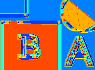
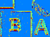
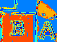
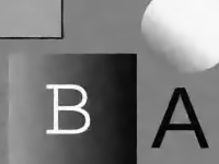
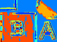
Figure 5: Sample denoising results for test image and $\sigma=20$. Each pixel in the color images indicates which of the $200$ gmm modes is assigned to each pixel in the corresponding image. The top row shows, from left to right: the clean image, its mode assignment map (this is the ground truth of the mode assignment problem), the noisy input, and the ground truth, again, for better comparison. The second row shows the first iterate of the denoised estimate obtained using paco, its corresponding mode map, the first iterate of epll, and its map. The last row shows the corresponding images for the 7th iterate of both algorithms (which is the last of epll). As can be seen, the results are very close and both final maps are close to the ground truth. However, on close inspection, the epll result has less artifacts and produces a softer cluster assignment.

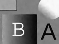
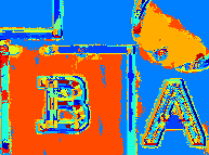
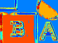
Figure 6: Comparison of denoising results obtained with the three paco-gmm variants on test image and $\sigma=20$. The first row is identical to that of Figure 5. The second and third rows correspond to the first and last iterates obtained using soft-thresholding ($\ell_{1}$) and dj for the estimates instead of the baseline ($\ell_{2}$) estimator of epll and paco-gmm. As can be seen, the results are significantly better, both in perceptive quality, and in terms of the estimated mode assignment.

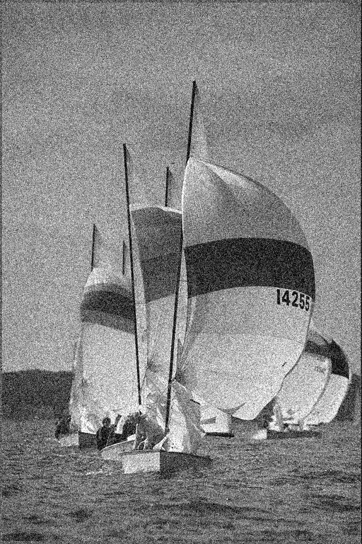
Figure 7: Visual comparison of results on the Kodak dataset and all variants tested (high resolution image – zoom for details). From top to bottom, left to right: noisy image (Kodim09 with $\sigma=30$), paco-gmm, epll, BM3D, paco-gmm-$\ell_{1}$ and paco-gmm-dj. The results in this case are clearly different between epll and paco-gmm. Furthermore, despite their relatively low performance in terms of rmse, the $\ell_{1}$ and dj variants produce less artifacts and overall a nicer result than any of the other methods (BM3D, which consistently yields the lower rmse, also exhibits more visible artifacts.)

5.7 Quantitative comparison

Table 2 summarizes the results obtained on the Kodak dataset, under three levels of noise, by the three variants of paco-gmm described above, epll, and BM3D. Figure 7 shows a visual comparison of these results on one of the Kodak images. Despite the similarities in terms of rmse, the results obtained with the different methods are clearly distinguishable. In particular, the $\ell_{1}$ and dj variants exhibit less artifacts. Moreover, BM3D, which is better in terms of rmse, tends to produce strong artifacts in smooth regions.

6 Contrast Enhancement

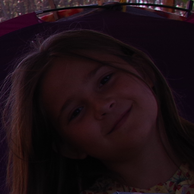
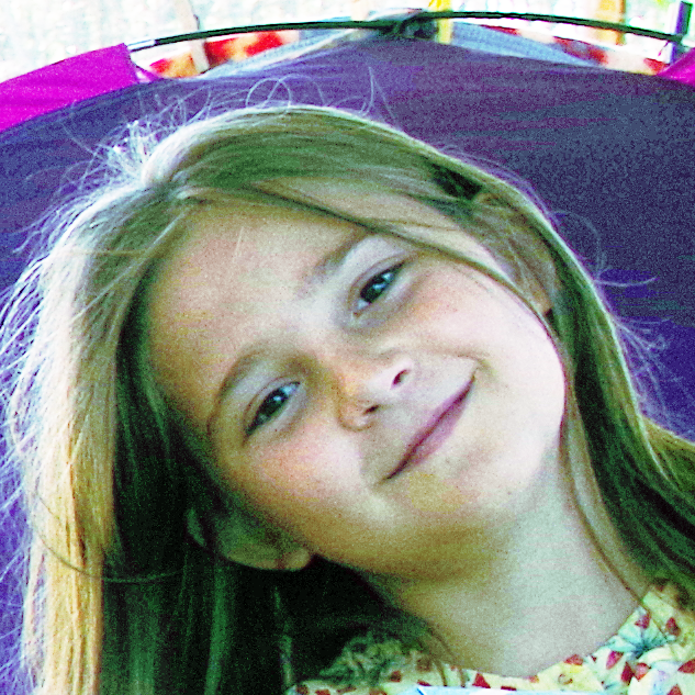
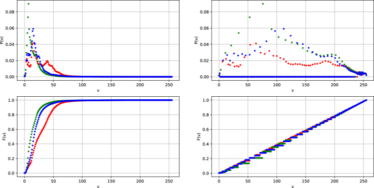
Figure 8: Global Histogram Equalization. Left, from top to bottom: original image, its histogram and cdf. Right: enhanced image, its histogram, and its cdf. In this case, the simple gce is enough to produce a significantly better image.

As a final example application we explore a problem where the cost function is not derived from a prior probability model on the patches. This is the case of the Local Contrast Enhancement (lce) problem: a now-ubiquitous post-processing image enhancement technique which generally provides better results than older and simpler Global Contrast Enhancement (gce) methods.

The basic method for improving the global contrast of an image is Histogram Equalization (heq): given an input image $\mathbf{{x}}$ taking on values in $[0,1)$, and the empirical cumulative distribution function of its values,

$$F_{\mathbf{{x}}}(z)=\frac{\sum_{i=1}^{N}\mathbf{1}(x_{i}<z)}{N},$$

the equalized image $\hat{\mathbf{{x}}}$ is obtained by the mapping

$$\hat{x}_{i}\leftarrow F_{x}^{-1}(x_{i}).$$

An example of this procedure is shown in Figure 8.

6.1 Contrast enhancement cost function

Let $(0\leq z_{1}<z_{2}<\ldots z_{k}\leq 1)$ be the $k$ different intensity levels occurring in $\mathbf{{x}}$. Histogram equalization can be seen as finding the corresponding levels in the enhanced image, $(\hat{z}_{1}<\ldots<\hat{z}_{k})$ which minimize the following cost function:

$$h(\hat{\mathbf{{x}}})=\int_{0}^{1}{(F_{\hat{\mathbf{{x}}}}(\mu)-\mu)}d\mu=\sum_{i=1}^{k+1}\int_{\hat{z}_{i-1}}^{\hat{z}_{i}}{(F_{\hat{\mathbf{{x}}}}(\mu)-\mu)}d\mu,$$

where we have defined $z_{0}=0$ and $z_{k+1}=1$. Let $(p_{1},p_{2},\ldots,p_{k})$ be the empirical probability distribution of each level in $\mathbf{{x}}$; this vector is not modified during minimization. We have that

$$F_{\hat{\mathbf{{x}}}}(\mu)=F_{i-1}=\sum_{r=1}^{i-1}p_{r},\;\hat{z}_{i-1}\leq\mu<\hat{z}_{i},$$

so that $F_{\hat{\mathbf{{x}}}}$ is constant within each integral and does not depend on $(\hat{z}_{1},\hat{z}_{2},\ldots,\hat{z}_{k})$. We define $F_{0}=0$. After integration, we obtain the following cost function on $(\hat{z}_{1},\hat{z}_{2},\ldots,\hat{z}_{k})$:

$$h(\hat{\mathbf{{x}}})=f(\hat{z}_{1},\hat{z}_{2},\ldots,\hat{z}_{k})=\sum_{i=1}^{k+1}\int_{\hat{z}_{i-1}}^{\hat{z}_{i}}{(F_{\hat{\mathbf{{x}}}}(\mu)-\mu)}d\mu=\sum_{i=1}^{k+1}\frac{1}{2}\left[\left(F_{i-1}-\hat{z}_{i}\right)^{2}-\left(F_{i-1}-\hat{z}_{i-1}\right)^{2}\right].$$

The solution to the above problem is given by

6.2 Local contrast enhancement

In certain situations, global contrast enhancement is not enough. Images such as the leftmost one in Figure 9, where large regions are subject to very different local luminosities, are not effectively improved by this method. As the name implies, local contrast enhancement works by correcting contrast in different regions. Two well known and very successful methods for this task are Retinex [34] and Automatic Color Enhancement (ace) [56]; see  [24] for a fast, free and open source implementation of ace. It should be noted that both Retinex and ace are not limited to contrast enhancement: Retinex also handles white balance, while ace handles contrast, white balance, and exposure automatically. The algorithm that we present next is limited only to contrast enhancement. Besides these well established methods, there are many other local contrast enhancements which have their own strengths, e.g. being faster, or being less sensitive to noise than the above ones [31, 37, 44, 47]. Many such methods are implemented in IPOL, see e.g. [21, 24, 27, 37, 50]; we invite the reader to experiment with these methods.

In this section we explore the simple idea of applying histogram equalization on a patch-wise basis to achieve local contrast while using paco to obtain a globally-coherent result. We do not claim our proposed method to be better than any of the aforementioned ones. In fact, it should hardly be the case, as many of them rely on carefully studied perceptual properties of human perception, whereas our method is conceptually very simple.

Because plain histogram equalization is usually very aggressive, we include an additional term to the cost function so that the result is a weighted average between the equalized result and the original patches. Also, in order to account include some exposure compensation capability (the so called gray world principle), we add an extra term which accounts for deviations of the mean patch value from the middle intensity $0.5$; the resulting cost function on a given patch is given by:

$$h_{\alpha,\beta}(\hat{\mathbf{{x}}}_{j})=\alpha\int_{0}^{1}{(F_{\hat{\mathbf{{x}}}}(\mu)-\mu)}d\mu+\frac{\beta}{2}\left\|\hat{\mathbf{{x}}}-\frac{1}{2}\mathbf{1}\right\|_{2}^{2}+\frac{1-\alpha-\beta}{2}\left\|\mathbf{{x}}-\hat{\mathbf{{x}}}\right\|_{2}^{2}.$$

The fidelity term $\|\mathbf{{x}}-\hat{\mathbf{{x}}}\|_{2}^{2}$ can also be written in terms of the $F_{i}$ and $\hat{z}_{i}$, so that we can write the cost function solely in terms of the output levels of the image patch:

$$h_{\alpha,\beta}(\hat{z}_{1},\hat{z}_{2},\ldots,\hat{z}_{k})=\frac{\alpha}{2}\sum_{i=1}^{k+1}\left[\left(F_{i-1}-\hat{z}_{i}\right)^{2}-\left(F_{i-1}-\hat{z}_{i-1}\right)^{2}\right]+\frac{\beta}{2}\sum_{i=1}^{k}p_{i}(\hat{z}_{i}-0.5)^{2}+\frac{1-\alpha}{2}\sum_{i=1}^{k}p_{i}(\hat{z}_{i}-z_{i})^{2}.$$ (25)

The solution to the above problem is

$$\hat{\mathbf{{x}}}=\alpha F^{-1}(\mathbf{{x}})+\beta\left(0.5-\frac{1}{N}\sum_{i}\mathbf{{x}}_{i}\right)\mathbf{1}+(1-\alpha-\beta)\mathbf{{x}}.$$ (26)

It is important to note that Eq. 25 includes a fidelity term with respect to the original input image $\mathbf{{x}}$. If we want to preserve its purpose, we cannot let this term depend on an image which is an iterate within the admm algorithm, as the original reference would be lost. Thus, in our implementation, the last term of Eq. 25 is always with respect to the input image, which is constant throughout the iterations. With this in mind, we now plug $h_{\alpha,\beta}(\cdot)$ in the paco framework to define our paco-heq problem:

$$\hat{\mathbf{{x}}}=\arg\min_{\zeta}h_{\alpha,\beta}(\zeta)+g(\zeta).$$

As in the denoising case, the splitting can be done in more than one way. We choose the following splitting, which is consistent with our definition of the problem:

$$(\hat{\mathbf{{x}}},\hat{\mathbf{{z}}})=\arg\min_{\zeta,\xi}h_{\alpha,\beta}(\zeta)+g(\xi)+\frac{1}{2\tau}\|\zeta-\xi\|_{2}^{2},\;\mathrm{s.t.}\;\zeta=\xi.$$

Following the standard procedure we have been using so far, the update $\hat{\mathbf{{y}}}^{(t+1)}$ given $\hat{\mathbf{{z}}}^{(t)}$ and $\mathbf{{u}}^{(t)}$ is obtained by applying the stitching trick to $\hat{\mathbf{{z}}}^{(t)}-\mathbf{{u}}^{(t)}$. The update on $\hat{\mathbf{{z}}}$ is given by

$$\hat{\mathbf{{z}}}^{(t+1)}\leftarrow\frac{\alpha}{1+\tau}F^{-1}\left[\hat{\mathbf{{y}}}^{(t+1)}-\mathbf{{u}}^{(t)}\right]+\frac{\beta}{1+\tau}\left[0.5-\frac{1}{N}\sum_{i}(\hat{\mathbf{{y}}}^{(t+1)}-\mathbf{{u}}^{(t)})_{i}\right]\mathbf{1}+\frac{1+\tau-\alpha-\beta}{1+\tau}\mathbf{{x}}.$$

Notice that the last term depends on the input $\mathbf{{x}}$, not on the iterate. In the patch-wise formulation, this is replaced by the original image patches vector $\mathbf{{y}}$. We summarize these steps in Algorithm 6.

Algorithm 6 PACO-HEQ algorithm.

0:  image $\mathbf{{x}}$, mixing ratios $0<\alpha,\beta<1$, admm parameter $\tau$

  $\mathbf{{y}}\leftarrow\mathbf{{R}}\mathbf{{x}}$

  $t\leftarrow 0$; $\hat{\mathbf{{y}}}^{(t)}\leftarrow\mathbf{{y}}$; $\mathbf{{u}}^{(t)}\leftarrow\mathbf{0}$

  repeat

     $\hat{\mathbf{{z}}}_{j}^{(t+1)}\leftarrow\frac{\alpha}{1+\tau}F^{-1}\left(\hat{\mathbf{{y}}}_{j}^{(t+1)}-\mathbf{{u}}_{j}^{(t)}\right)+\frac{\beta}{1+\tau}\left[0.5-\frac{1}{N}\sum_{i}(\hat{\mathbf{{y}}}_{j}^{(t+1)}-\mathbf{{u}}_{j}^{(t)})\right]\mathbf{1}+\frac{1+\tau-\alpha-\beta}{1+\tau}\mathbf{{y}}_{j}\,,\;j=1,\ldots,n$

     $\hat{\mathbf{{y}}}^{(t+1)}\leftarrow\mathbf{{R}}(\mathbf{{R}}^{\intercal}\mathbf{{R}})^{-1}\mathbf{{R}}^{\intercal}(\hat{\mathbf{{z}}}^{(t+1)}+\mathbf{{u}}^{(t)})$

     $\mathbf{{u}}^{(t+1)}\leftarrow\mathbf{{u}}^{(t)}+\hat{\mathbf{{y}}}^{(t+1)}-\hat{\mathbf{{z}}}^{(t+1)}$

     $t\leftarrow t+1$

  until convergence

  return  enhanced image $\hat{\mathbf{{x}}}\leftarrow\mathbf{{R}}^{\intercal}\hat{\mathbf{{y}}}^{(t)}$

6.3 Sample results

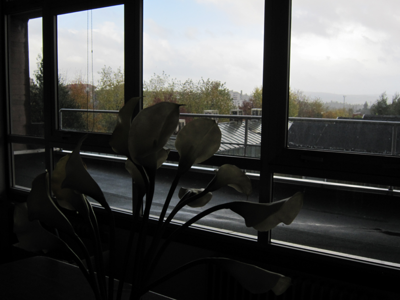
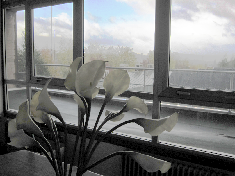
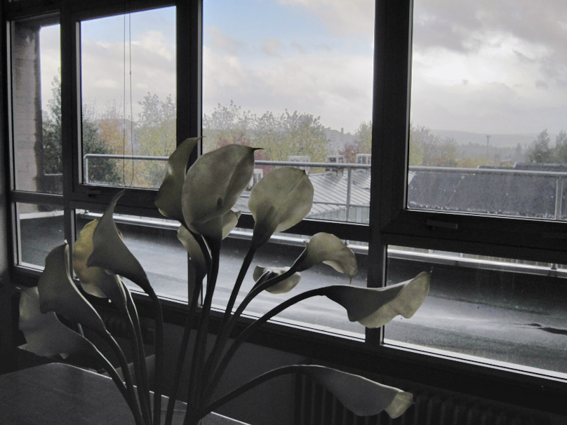
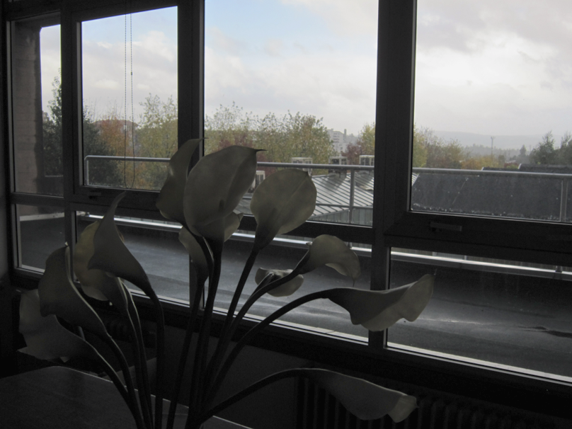
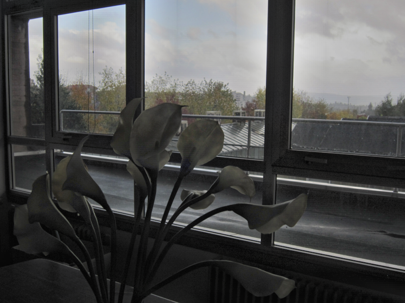
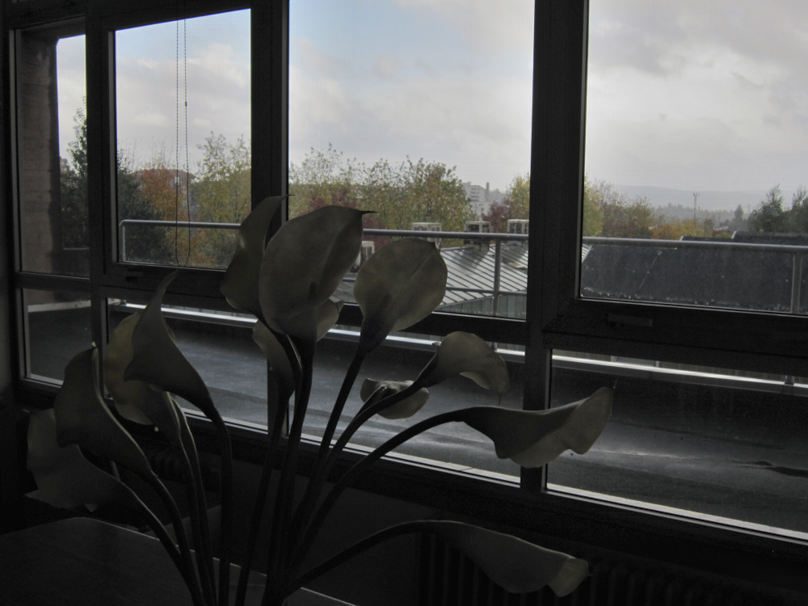
Figure 9: Contrast Enhancement results on Iris image. Top row: original image, global heq, ace with $\alpha=8$. Bottom row: paco-heq equalization function Eq. 26 with $\alpha=0.25$ and $\beta=0.05$ applied globally, paco-heq with same parameters on patches of size $64{\times}64$ and stride $8$, paco-heq obtained with the same parameters except $\alpha=0.125$ (less contrast). Differences are particularly noticeable in the leaves of the plant.

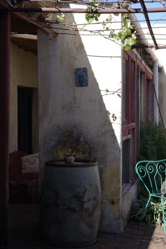
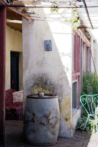
Figure 10: Contrast Enhancement results on Barril image. Left to right: original image, global HEQ, ACE with $\alpha=8$, paco-heq with $\alpha=0.25$,$\beta=0.05$, patches of size $64{\times}64$ and a stride of $s=8$.

Sample results are shown in Figure 9 and Figure 10. Overall, with these parameters, paco-heq does produce a noticeable improvement in local contrast. It tends to preserve the local intensity more than the other methods, but still produces significantly sharper results. The source code, as well as more examples, can be found in http://iie.fing.edu.uy/~nacho/paco/.

7 Concluding remarks and future work

We have presented paco, a general framework for solving signal restoration problems under a patch consensus constraint. We have shown that the resulting optimization problem is feasible and easy to solve using the standard admm method. In particular, we described a general and practical solution to the patch reprojection step, named the “stitching trick”, which sidesteps the major bottleneck in similar methods. We have also shown that the hard consensus constraint allows for the definition of constraints directly in signal space, which may allow for new ways of formulating old problems.

The paco framework was showcased in three sample applications with good results, both in terms of quality and efficiency. Several other applications are possible; we are already working on a few of them, the results of which will be published elsewhere.

Besides new applications, paco can also be used as a platform for distributed processing of very large images, by letting different nodes process smaller sub-images and then using the consensus mechanism to merge the results. In fact, distributed computing applications and network optimization are the fields where consensus optimization problems, as described in section 3, were first analyzed.

Finally, the patch consensus idea can be extended in various ways. For example, it could be used in combination with the classic mixture of experts or boosting as a way to combine the output of the experts in a meaningful way. Another interesting extension would be a true multiscale patch consensus framework (our current framework readily allows for schemes such as dilated convolutions [63]).

References

- [1] C. Aguerrebere, A. Almansa, J. Delon, Y. Gousseau, and P. Musé, A bayesian hyperprior approach for joint image denoising and interpolation, with an application to hdr imaging, IEEE Transactions on Computational Imaging, 3 (2017), pp. 633–646, https://doi.org/10.1109/TCI.2017.2704439.
- [2] M. Aharon, M. Elad, and A. Bruckstein, K-SVD: An algorithm for designing overcomplete dictionaries for sparse representation, IEEE Transactions on Signal Processing, 54 (2006), pp. 4311–4322, https://doi.org/10.1109/TSP.2006.881199.
- [3] M. H. Alkinani and M. R. El-Sakka, Patch-based models and algorithms for image denoising: a comparative review between patch-based images denoising methods for additive noise reduction, Eurasip Journal on Image and Video Processing, 2017 (2017), www.scopus.com.
- [4] P. Arias, G. Facciolo, V. Caselles, and G. Sapiro, A variational framework for exemplar-based image inpainting, Int. J. Comput. Vision, 93 (2011), pp. 319–347, https://doi.org/10.1007/s11263-010-0418-7, http://dx.doi.org/10.1007/s11263-010-0418-7.
- [5] D. Batenkov, Y.Romano, and M. Elad, On the Global-Local Dichotomy in Sparsity Modeling, Springer International Publishing, Cham, 2017, pp. 1–53, https://doi.org/10.1007/978-3-319-69802-1_1, https://doi.org/10.1007/978-3-319-69802-1_1.
- [6] F. Bornemann and T. März, Fast image inpainting based on coherence transport, J. Math. Imaging Vis., 1 (2007), pp. 259–278.
- [7] K. Brandt, M. Syskind, J. Larsen, K. Strimmer, L. Christiansen, J. Hansen, L. He, L. Thibaut, M. Barão, S. Hattinger, V. Sima, and W. The, The matrix cookbook – version 12, tech. report, Technical University of Denmark, 2012.
- [8] H. Bristow, A. Eriksson, and S. Lucey, Fast convolutional sparse coding, in 2013 IEEE Conference on Computer Vision and Pattern Recognition, 2013, pp. 391–398, https://doi.org/10.1109/CVPR.2013.57.
- [9] A. Buades, B. Coll, and J. Morel, A review of image denoising algorithms, with a new one, Multiscale Modeling & Simulation, 4 (2005), pp. 490–530, https://doi.org/10.1137/040616024, https://doi.org/10.1137/040616024, https://arxiv.org/abs/https://doi.org/10.1137/040616024.
- [10] T. F. Chan and J. Shen, Image Processing and Analysis: Variational, PDE, Wavelet, and Stochastic Methods, Society for Industrial and Applied Mathematics (SIAM). Philadelphia, PA., 2005.
- [11] K. Dabov, A. Foi, V. Katkovnik, and K. Egiazarian, Image denoising by sparse 3-d transform-domain collaborative filtering, IEEE Transactions on Image Processing, 16 (2007), pp. 2080–2095, https://doi.org/10.1109/TIP.2007.901238.
- [12] I. Daubechies, The wavelet transform, time-frequency localization and signal analysis, IEEE Transactions on Information Theory, 36 (1990), pp. 961–1005, https://doi.org/10.1109/18.57199.
- [13] Z. Dengwen and S. Xiaoliu, Image denoising using weighted averaging, in 2009 WRI International Conference on Communications and Mobile Computing, vol. 1, Jan 2009, pp. 400–403, https://doi.org/10.1109/CMC.2009.64.
- [14] D. L. Donoho and I. M. Johnstone, Ideal spatial adaptation by wavelet shrinkage, Biometrika, 81 (1994), pp. 425–455, https://doi.org/10.1093/biomet/81.3.425, https://doi.org/10.1093/biomet/81.3.425, https://arxiv.org/abs/https://academic.oup.com/biomet/article-pdf/81/3/425/26079146/81.3.425.pdf.
- [15] J. Eckstein and D. Bertsekas, On the Douglas-Rachford splitting method and the proximal point algorithm for maximal monotone operators, Mathematical Programming, 55 (1992), pp. 293–318, https://doi.org/https://doi.org/10.1007/BF01581204.
- [16] M. Elad and M. Aharon, Image denoising via sparse and redundant representations over learned dictionaries, IEEE Transactions on Image Processing, 15 (2006).
- [17] K. Engan, S. Aase, and J. Husoy, Multi-frame compression: Theory and design, Signal Processing, 80 (2000), pp. 2121–2140.
- [18] E. Esser, X. Zhang, and T. Chan, A general framework for a class of first order primal-dual algorithms for convex optimization in imaging science, SIAM Journal on Imaging Sciences, 3 (2010), pp. 1015–1046.
- [19] V. Fedorov, G. Facciolo, and P. Arias, Variational Framework for Non-Local Inpainting, Image Processing On Line, 5 (2015), pp. 362–386, https://doi.org/10.5201/ipol.2015.136.
- [20] J. Feng, L. Song, X. Huo, X. Yang, and W. Zhang, An optimized pixel-wise weighting approach for patch-based image denoising, IEEE Signal Processing Letters, 22 (2015), pp. 115–119, https://doi.org/10.1109/LSP.2014.2350032.
- [21] S. Ferradans, R. Palma-Amestoy, and E. Provenzi, An Algorithmic Analysis of Variational Models for Perceptual Local Contrast Enhancement, Image Processing On Line, 5 (2015), pp. 219–233. https://doi.org/10.5201/ipol.2015.131.
- [22] M. A. T. Figueiredo, Synthesis versus analysis in patch-based image priors, in 2017 IEEE International Conference on Acoustics, Speech and Signal Processing (ICASSP), March 2017, pp. 1338–1342, https://doi.org/10.1109/ICASSP.2017.7952374.
- [23] D. Geman and C. Yang, Nonlinear image recovery with half-quadratic regularization, IEEE Trans. Image Process., 4 (1995), pp. 932–946.
- [24] P. Getreuer, Automatic Color Enhancement (ACE) and its Fast Implementation, Image Processing On Line, 2 (2012), pp. 266–277. https://doi.org/10.5201/ipol.2012.g-ace.
- [25] P. Getreuer, Total Variation Inpainting using Split Bregman, Image Processing On Line, 2 (2012), pp. 147–157, https://doi.org/10.5201/ipol.2012.g-tvi.
- [26] V. Gnann and J. Becker, Signal reconstruction from multiresolution STFT magnitudes with mutual initialization, in Proceedings of the AES International Conference, 2012, pp. 274–279, www.scopus.com.
- [27] J. G. Gomila and J. L. Lisani, Local Color Correction, Image Processing On Line, 1 (2011), pp. 260–280. https://doi.org/10.5201/ipol.2011.gl_lcc.
- [28] M. M. Goodwin, Realization of arbitrary filters in the STFT domain, in IEEE Workshop on Applications of Signal Processing to Audio and Acoustics, 2009, pp. 353–356, www.scopus.com. Cited By :1.
- [29] O. G. Guleryuz, Weighted averaging for denoising with overcomplete dictionaries, IEEE Transactions on Image Processing, 16 (2007), pp. 3020–3034, https://doi.org/10.1109/TIP.2007.908078.
- [30] S. Hurault, T. Ehret, and P. Arias, EPLL: An Image Denoising Method Using a Gaussian Mixture Model Learned on a Large Set of Patches, Image Processing On Line, 8 (2018), pp. 465–489. https://doi.org/10.5201/ipol.2018.242.
- [31] D. Jobson, Z. Rahman, and G. Woodell, A multiscale retinex for bridging the gap between color images and the human observation of scenes, IEEE Trans. Image Process., 6 (1997), pp. 965–976, https://doi.org/http://dx.doi.org/10.1109/83.597272.
- [32] N. Kawai, T. Sato, and N. Yokoya, Image inpainting considering brightness change and spatial locality of textures and its evaluation, in Advances in Image and Video Technology, T. Wada, F. Huang, and S. Lin, eds., Berlin, Heidelberg, 2009, Springer Berlin Heidelberg, pp. 271–282.
- [33] C. Kervrann and J. Boulanger, Optimal spatial adaptation for patch-based image denoising, IEEE Trans. Image Process., 15 (2006), pp. 2866–2878.
- [34] E. Land and J. McCann, Lightness and retinex theory, Journal of the Optical Society of America, 61 (1971), pp. 1–11, https://doi.org/http://dx.doi.org/10.1364/JOSA.61.000001.
- [35] J. Le Roux, H. Kameoka, N. Ono, and S. Sagayama, Fast signal reconstruction from magnitude STFT spectrogram based on spectrogram consistency, in 13th International Conference on Digital Audio Effects, DAFx 2010 Proceedings, 2010, www.scopus.com. Cited By :29.
- [36] M. Lewicki and B. Olshausen, Probabilistic framework for the adaptation and comparison of image codes, J. Opt. Soc. Am. A, 16 (1999), pp. 1587–1601, http://josaa.osa.org/abstract.cfm?URI=josaa-16-7-1587.
- [37] J. L. Lisani, A. B. Petro, and C. Sbert, Color and Contrast Enhancement by Controlled Piecewise Affine Histogram Equalization, Image Processing On Line, 2 (2012), pp. 243–265. https://doi.org/10.5201/ipol.2012.lps-pae.
- [38] Z. Liu, L. Chen, and J. Yang, An image reconstruction algorithm using patch-based locally optimal wiener filtering, Dianzi Yu Xinxi Xuebao/Journal of Electronics and Information Technology, 36 (2014), pp. 2556–2562, www.scopus.com. Cited By :3.
- [39] J. Mairal, F. Bach, J. Ponce, and G. Sapiro, Online learning for matrix factorization and sparse coding, Journal of Machine Learning Research, 11 (2010), pp. 19–60, www.scopus.com. Cited By :1302.
- [40] J. Mairal, M. Elad, and G. Sapiro, Sparse representation for color image restoration, IEEE Transactions on Image Processing, 17 (2008), pp. 53–69, www.scopus.com. Cited By :930.
- [41] J. Mairal, G. Sapiro, and M. Elad, Learning multiscale sparse representations for image and video restoration, Multiscale Modeling and Simulation, 7 (2008), pp. 214–241, www.scopus.com. Cited By :285.
- [42] S. G. Mallat, A theory for multiresolution signal decomposition: the wavelet representation, IEEE Transactions on Pattern Analysis and Machine Intelligence, 11 (1989), pp. 674–693, https://doi.org/10.1109/34.192463.
- [43] J. A. Moorer, A note on the implementation of audio processing by Short-Term Fourier Transform, in IEEE Workshop on Applications of Signal Processing to Audio and Acoustics, vol. 2017-October, 2017, pp. 156–159, www.scopus.com.
- [44] N. Moroney, Local color correction using non-linear masking, in IS&T/SID Eight Color Imaging Conference, 2000, pp. 108–111.
- [45] G. Motta, E. Ordentlich, I. Ramirez, G. Seroussi, and M. J. Weinberger, The iDUDE framework for grayscale image denoising, IEEE Transactions on Image Processing, 20 (2011), pp. 1–21, https://doi.org/10.1109/TIP.2010.2053939.
- [46] A. Newson, A. Almansa, Y. Gousseau, and P. Pérez, Non-Local Patch-Based Image Inpainting, Image Processing On Line, 7 (2017), pp. 373–385, https://doi.org/10.5201/ipol.2017.189.
- [47] R. Palma-Amestoy, E. Provenzi, M. Bertalmío, and V. Caselles, A perceptually inspired variational framework for color enhancement, IEEE Transactions on Pattern Analysis and Machine Intelligence, 31 (2009), pp. 458–474, https://doi.org/10.1109/TPAMI.2008.86.
- [48] V. Papyan and M. Elad, Multi-scale patch-based image restoration, IEEE Transactions on Image Processing, 25 (2016), pp. 249–261, www.scopus.com.
- [49] N. Parikh and S. P. Boyd, Proximal algorithms, Foundations and Trends in Optimization, 1 (2014), pp. 127–239, https://doi.org/10.1561/2400000003, https://doi.org/10.1561/2400000003.
- [50] A. B. Petro, C. Sbert, and J.-M. Morel, Multiscale Retinex, Image Processing On Line, (2014), pp. 71–88. https://doi.org/10.5201/ipol.2014.107.
- [51] G. Peyré, Image processing with nonlocal spectral bases, Multiscale Modeling & Simulation, 7 (2008), pp. 703–730, https://doi.org/10.1137/07068881X, https://doi.org/10.1137/07068881X, https://arxiv.org/abs/https://doi.org/10.1137/07068881X.
- [52] G. Peyré, Manifold models for signals and images, Computer Vision and Image Understanding, 113 (2009), pp. 249–260, https://doi.org/https://doi.org/10.1016/j.cviu.2008.09.003, https://www.sciencedirect.com/science/article/pii/S1077314208001550.
- [53] I. Ramirez and G. Sapiro, Universal regularizers for robust sparse coding and modeling, IEEE Transactions on Image Processing, 21 (2012), pp. 3850–3864, https://doi.org/10.1109/TIP.2012.2197006.
- [54] I. Ramírez and I. Hounie, Paco and paco-dct: Patch consensus and its application to inpainting, in ICASSP 2020 - 2020 IEEE International Conference on Acoustics, Speech and Signal Processing (ICASSP), 2020, pp. 5775–5779, https://doi.org/10.1109/ICASSP40776.2020.9053953.
- [55] I. Ramírez and I. Hounie, Image Inpainting using Patch Consensus and DCT Priors, Image Processing On Line, 11 (2021), pp. 1–17. https://doi.org/10.5201/ipol.2021.286.
- [56] A. Rizzi, C. Gatta, and D. Marini, A new algorithm for unsupervised global and local color correction, Pattern Recognition Letters, 24 (2003), pp. 1663–1677, https://doi.org/https://doi.org/10.1016/S0167-8655(02)00323-9, https://www.sciencedirect.com/science/article/pii/S0167865502003239. Colour Image Processing and Analysis. First European Conference on Colour in Graphics, Imaging, and Vision (CGIV 2002).
- [57] Y. Romano and M. Elad, Patch-disagreement as away to improve K-SVD denoising, in 2015 IEEE International Conference on Acoustics, Speech and Signal Processing (ICASSP), April 2015, pp. 1280–1284, https://doi.org/10.1109/ICASSP.2015.7178176.
- [58] A. Saint-Dizier, J. Delon, and C. Bouveyron, A unified view on patch aggregation, Journal of Mathematical Imaging and Vision, 62 (2020), pp. 149–168, https://doi.org/10.1007/s10851-019-00921-z, https://doi.org/10.1007/s10851-019-00921-z.
- [59] O. G. Sezer and Y. Altunbasak, Weighted average denoising with sparse orthonormal transforms, in 2009 16th IEEE International Conference on Image Processing (ICIP), Nov 2009, pp. 3849–3852, https://doi.org/10.1109/ICIP.2009.5414056.
- [60] C. M. Stein, Estimation of the Mean of a Multivariate Normal Distribution, The Annals of Statistics, 9 (1981), pp. 1135 – 1151, https://doi.org/10.1214/aos/1176345632, https://doi.org/10.1214/aos/1176345632.
- [61] B. Wang, T. Lu, and Z. Xiong, Adaptive boosting for image denoising: Beyond low-rank representation and sparse coding, in 2016 23rd International Conference on Pattern Recognition (ICPR), Dec 2016, pp. 1400–1405, https://doi.org/10.1109/ICPR.2016.7899833.
- [62] Y.-Q. Wang and J.-M. Morel, Sure guided gaussian mixture image denoising, SIAM Journal on Imaging Sciences, 6 (2013), pp. 999–1034, https://doi.org/10.1137/120901131, https://doi.org/10.1137/120901131, https://arxiv.org/abs/https://doi.org/10.1137/120901131.
- [63] F. Yu and V. Koltun, Multi-scale context aggregation by dilated convolutions, in 4th International Conference on Learning Representations, ICLR 2016, San Juan, Puerto Rico, May 2-4, 2016, Conference Track Proceedings, Y. Bengio and Y. LeCun, eds., 2016, http://arxiv.org/abs/1511.07122.
- [64] G. Yu and G. Sapiro, DCT Image Denoising: a Simple and Effective Image Denoising Algorithm, Image Processing On Line, 1 (2011), pp. 292–296. https://doi.org/10.5201/ipol.2011.ys-dct.
- [65] G. Yu, G. Sapiro, and S. Mallat, Solving inverse problems with piecewise linear estimators: From gaussian mixture models to structured sparsity, IEEE Transactions on Image Processing, 21 (2012), pp. 2481–2499.
- [66] D. Zoran and Y. Weiss, From learning models of natural image patches to whole image restoration, in 2011 International Conference on Computer Vision, Nov 2011, pp. 479–486, https://doi.org/10.1109/ICCV.2011.6126278.