Long time asymptotics for homoenergetic solutions of the Boltzmann equation. Collision-dominated case.

Abstract

In this paper we present a formal analysis of the long-time asymptotics of a particular class of solutions of the Boltzmann equation, known as homoenergetic solutions, which have the form $f\left(x,v,t\right)=g\left(v-L\left(t\right)x,t\right)$ where $L\left(t\right)=A\left(I+tA\right)^{-1}$ with the matrix $A$ describing a shear flow or a dilatation or a combination of both. We began this study in [18]. Homoenergetic solutions satisfy an integro-differential equation which contains, in addition to the classical Boltzmann collision operator, a linear hyperbolic term. In [18] it has been proved rigorously the existence of self-similar solutions which describe the change of the average energy of the particles of the system in the case in which there is a balance between the hyperbolic and the collision term.

In this paper we focus in homoenergetic solutions for which the collision term is much larger than the hyperbolic term (collision-dominated behavior). In this case the long time asymptotics for the distribution of velocities is given by a time dependent Maxwellian distribution with changing temperature.

1 Introduction

In this paper we study the long time asymptotics of a class of non self-similar solutions of the Boltzmann equation. The self-similar case was considered in [18]. The class of solutions under consideration is motivated by an invariant manifold of solutions of the equations of classical molecular dynamics with certain symmetry properties ([9, 10]).

As background, we recall briefly the properties of this manifold which have been summarized also in [18]. Given a matrix $A\in M_{3\times 3}\left(\mathbb{R}\right)$, and linearly independent vectors $e_{1},e_{2},e_{3}$ in $\mathbb{R}^{3}$, we consider a time interval $[0,a)$ such that $\det(I+tA)>0$ for $t\in[0,a)$ with $a>0$. We consider any number of atoms labeled $1,\dots,M$ with positive masses $m_{1},\dots,m_{M}$ and initial conditions

$${y}_{k}(0)={y}_{k}^{0},\quad\dot{y}_{k}(0)={v}_{k}^{0},\quad k=1,\dots,M.$$ (1.1)

These $M$ atoms will be called simulated atoms. The simulated atoms will be subject to the equations of molecular dynamics (to be stated presently) with the initial conditions (1.1), yielding solutions $y_{k}(t)\in\mathbb{R}^{3},\ 0\leq t<a,\ k=1,\dots,M$. In addition there will be non-simulated atoms with time-dependent positions $y_{\nu,k}(t)$, indexed by a triple of integers $\nu=(\nu_{1},\nu_{2},\nu_{3})\in\mathbb{Z}^{3},\ \nu\neq(0,0,0)$ and $k=1,\dots,M$. The nonsimulated atom $(\nu,k)$ will have mass $m_{k}$. The positions of the nonsimulated atoms will be given by the following explicit formulas based on the positions of the simulated atoms:

$$y_{\nu,k}(t)=y_{k}(t)+(I+tA)(\nu_{1}e_{1}+\nu_{2}e_{2}+\nu_{3}e_{3}),\quad\nu=(\nu_{1},\nu_{2},\nu_{3})\in\mathbb{Z}^{3},\ k=1,\dots,M.$$ (1.2)

For $k=1,\dots,M$ we denote as $f_{k}:\cdots\mathbb{R}^{3}\times\mathbb{R}^{3}\times{\mathbb{R}^{3}}\cdots\rightarrow\mathbb{R}$ the force on simulated atom $k$. The force on simulated atom $k$ depends on the positions of all the atoms. We assume that the force $f_{k}$ satisfies the usual conditions of frame-indifference and permutation invariance [9]. Then, the dynamics of the simulated atoms is given by:

$$m_{k}\ddot{y}_{k} =f_{k}(\dots,y_{\nu_{1},1},\dots,y_{\nu_{1},M},\dots,y_{\nu_{2},1},\dots,y_{\nu_{2},M},\dots),$$ (1.3)

$${y}_{k}(0) ={y}_{k}^{0},\quad\dot{y}_{k}(0)={v}_{k}^{0},\quad k=1,\dots,M.$$

Notice that these equations can be reduced to standard ODEs for the motions of the simulated atoms substituting the formulas (1.2) into the right hand side of (1.3). It is shown in [9] and [10] that in spite of the fact that the motions of the nonsimulated atoms are only given by the formulas (1.2), the equations of molecular dynamics (1.3) are exactly satisfied for each nonsimulated atom. Further information is also given in [18]. As discussed there, these results on molecular dynamics have a simple interpretation in terms of the molecular density function of the kinetic theory. To explain this interpretation we recall that the classical Boltzmann equation has the form

$$\partial_{t}f+v\partial_{x}f =\mathbb{C}f\left(v\right)\ \ ,\ \ f=f\left(t,x,v\right)$$

$$\mathbb{C}f\left(v\right) =\int_{\mathbb{R}^{3}}dv_{\ast}\int_{S^{2}}d\omega B\left(n\cdot\omega,\left|v-v_{\ast}\right|\right)\left[f^{\prime}f_{\ast}^{\prime}-f_{\ast}f\right],\$$ (1.4)

where $S^{2}$ is the unit sphere in $\mathbb{R}^{3}$ and $n=n\left(v,v_{\ast}\right)=\frac{\left(v-v_{\ast}\right)}{\left|v-v_{\ast}\right|}.$ Here $(v,v_{\ast})$ is a pair of velocities in incoming collision configuration (see Figure 1) and $(v^{\prime},v_{\ast}^{\prime})$ is the corresponding pair of outgoing velocities defined by the collision rule

$$v^{\prime} =v+\left(\left(v_{\ast}-v\right)\cdot\omega\right)\omega,$$ (1.5)

$$v_{\ast}^{\prime} =v_{\ast}-\left(\left(v_{\ast}-v\right)\cdot\omega\right)\omega.$$ (1.6)

The unit vector $\omega=\omega(v,V)$ bisects the angle between the incoming relative velocity $V=v_{\ast}-v$ and the outgoing relative velocity $V^{\prime}=v_{\ast}^{\prime}-v^{\prime}$ as specified in Figure 1. The collision kernel $B\left(n\cdot\omega,\left|v-v_{\ast}\right|\right)$ is proportional to the cross section for the scattering problem associated to the collision between two particles. We use the conventional notation in kinetic theory, $f=f\left(t,x,v\right),\ f_{\ast}=f\left(t,x,v_{\ast}\right),\ f^{\prime}=f\left(t,x,v^{\prime}\right),\ \ f_{\ast}^{\prime}=f\left(t,x,v_{\ast}^{\prime}\right)$.

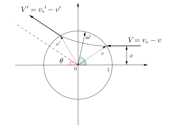
Figure 1: The two-body scattering. The solution of the two-body problem lies in a plane, which is taken to be the plane of the page, and the motion of molecule $\ast$ is plotted relative to the unstarred molecule. The scalar $\rho$ is the impact parameter expressed in microscopic units, $\rho\in[-1,1]$, and $\theta=\theta(\rho,|V|)$ is the scattering angle. The scattering vector of (1.5), (1.6) is the unit vector $\omega=\omega(v,V)$.

We will assume that the kernel $B$ is homogeneous with respect to the variable $\left|v-v_{\ast}\right|$ and we will denote its homogeneity by $\gamma,\$i.e.,

$$B\left(n\cdot\omega,\lambda\left|v-v_{\ast}\right|\right)=\lambda^{\gamma}B\left(n\cdot\omega,\left|v-v_{\ast}\right|\right),\ \ \lambda>0.$$ (1.7)

It is possible to find solutions of the Boltzmann equation (1.4) in the same spirit of the molecular dynamics simulation for discrete systems described above (see (1.2)). Indeed, let us consider a ball $B_{r}(x)$ of any radius $r$ centered at $x=(I+tA)(\nu_{1}e_{1}+\nu_{2}e_{2}+\nu_{3}e_{3})$, $(\nu_{1},\nu_{2},\nu_{3})\in\mathbb{Z}^{3}$. The ansatz (1.2) implies that, the velocities of the atoms in the ball $B_{r}(x)$ are determined by those in the ball $B_{r}(0)$ by the time derivative of (1.2). The molecular density function $f(t,x,v)$ of the kinetic theory describes the probability density of finding velocities in the small neighborhood of a point $x$ at time $t$. Thus, the ansatz above for the particle velocities in the balls $B_{r}(x)$ can be written down using (1.2) and its time-derivative as:

$$f(t,x,v)=g(t,v-A(I+tA)^{-1}x).$$ (1.8)

The term $A(I+tA)^{-1}$ arises from conversion to the Eulerian form of the kinetic theory.

The study of solutions of kinetic equations with the form (1.8) is also interesting from the general perspective of non-equilibrium statistical mechanics. We have shown in [18] that for broad classes of choices of $A$, there exist solutions of the Boltzmann equation satisfying (1.8). We have obtained also explicit formulas for the entropy of some of these solutions in terms of the time-dependent temperature and density.

An alternative viewpoint based on the theory of equidispersive solutions and leading to the same result is presented in Section 2. These are solutions of the Boltzmann equation with the form

$$f\left(t,x,v\right)=g\left(t,w\right)\text{ \ \ with }w=v-\xi\left(t,x\right).\$$ (1.9)

Under mild smoothness conditions, solutions with the form (1.9) exist if and only if $\xi(t,x)=A(I+tA)^{-1}x$. Formally, if $f$ is a solution of the Boltzmann equation (1.4) of the form (1.8) the function $g$ satisfies

$$\partial_{t}g-\big{(}L\left(t\right)w\big{)}\cdot\partial_{w}g=\mathbb{C}g\left(w\right)$$ (1.10)

where the collision operator $\mathbb{C}$ is defined as in (1.4). These solutions are called homoenergetic solutions and were introduced by Galkin [12] and Truesdell [25].

Homoenergetic solutions of the Boltzmann equation have been studied in [1], [2], [3], [5], [6], [7], [12], [13], [14], [15], [22], [23], [25], [26]. Details about the precise contents of these papers will be given later in the corresponding sections where related results appear.

The properties of the solutions of (1.10) for large time $t$ depends sensitively on the homogeneity of the kernel yielding the cross section of the collision operator $\mathbb{C}g.$ In [18] we have focused on the analysis of solutions of (1.10) for which the terms $L\left(t\right)w\cdot\partial_{w}g$ and $\mathbb{C}g\left(w\right)$ are comparable. This happens for most choices of the matrix $A$ if the homogeneity $\gamma=\frac{\nu-5}{\nu-1}$ of the cross section appearing in the operator $\mathbb{C}g\left(w\right)$ is zero, that is, for potentials of the form $V\left(x\right)=\frac{1}{\left|x\right|^{\nu-1}}$ with $\nu=5$. It is customary in this case to say that the particles described by the distribution $f$ in (1.9) are Maxwell molecules.

The main result that has been obtained in [18] is the rigorous proof of existence of self-similar solutions in the class of homoenergetic flows if the collision kernel describes the interaction between Maxwell molecules. In all the cases when such self-similar solutions exist, the terms $L\left(t\right)w\cdot\partial_{w}g$ and $\mathbb{C}g\left(w\right)$ have a comparable size as $t\rightarrow\infty.$

In this paper we will focus in the analysis of the possible long time asymptotics of the solutions of (1.10) in the cases in which the collision kernel describes the interactions between non Maxwellian molecules. This behavior strongly depends on the homogeneity of the collision kernel $B$ and on the particular form of the hyperbolic terms in the equation for the equidispersive flows, namely $L\left(t\right)w\cdot\partial_{w}g$. We will see that depending on the homogeneity of the kernel we will have different possible solutions of the Boltzmann equations for large time. We have solutions for which the collision term $\mathbb{C}g\left(w\right)$ becomes the largest one as $t\rightarrow\infty.$ These solutions are approximately Maxwellians, with a time-dependent temperature. The differential equations which describe the evolution of the temperature can be obtained by means of a suitable adaptation of the standard Hilbert expansion. The description of this family of solutions, that we will denote as the collision-dominated case, is the main content of this paper.

Conversely, there are also choices of $L\left(t\right)$ and collision kernels $B$ for which the scaling properties of the different terms imply that the hyperbolic terms are much more important than the collision terms. We will refer to these solutions as hyperbolic-dominated case. This case is discussed in [19].

The molecular dynamic simulation method described above can be rephrased as an invariant manifold of the equations of molecular dynamics. Our existence result in [18], and other results in [19] and this paper show that this manifold is inherited faithfully by the Boltzmann equation. Our long term hope is to be able to write a relatively simple but general asymptotic statistics on this manifold. One could conjecture that the situation is like the equilibrium case, where the relevant manifold is ${\cal H}=const.$ (${\cal H}$ is the Hamiltonian), the “statistics” is the Maxwellian distribution (or, more generally, the Gibbs measure), and macroscopic properties are obtained as moments. Taken together, our results of [18], [19] and this paper on the dichotomy between hyperbolic-dominated and collision-dominated behavior suggest that our asymptotic statistics is quite simple, but not governed by single distribution as in the equilibrium case. In particular, the selection of asymptotic distribution is sensitively dependent on the growth (i.e., repulsiveness) of the atomic forces.

The plan of the paper is the following. In Section 2 we recall the main properties of homoenergetic solutions of the Boltzmann equation which have been obtained in [18]. In Section 3 we describe general conditions under which the homoenergetic solutions exist. Section 4 describes several choices of matrices $L\left(t\right)$ and collision kernels $B$ for which the long time asymptotics of the solutions is given by means of Hilbert expansions, or more precisely perturbations of the Maxwellian distribution with changing temperature. This section contains first a general theorem yielding Hilbert expansions for a large class of matrices $L\left(t\right)$ and collision kernels $B.$ This abstract result is then applied to specific choices of homoenergetic flows. In Section 5, we summarize the main results obtained in this paper, together with those given in [18], [19], and we write some concluding remarks.

2 Homoenergetic solutions of the Boltzmann equation

We consider the molecular density function $f\left(t,x,v\right)$ solution of (1.4), i.e. of

$$\partial_{t}f+v\partial_{x}f =\mathbb{C}f\left(v\right)\ \ ,\ \ f=f\left(t,x,v\right)$$

$$\mathbb{C}f\left(v\right) =\int_{\mathbb{R}^{3}}dv_{\ast}\int_{S^{2}}d\omega B\left(n\cdot\omega,\left|v-v_{\ast}\right|\right)\left[f^{\prime}f_{\ast}^{\prime}-f_{\ast}f\right].\$$

Formally, we can compute the density $\rho$, the average velocity $V$ and the internal energy $\varepsilon$ at each point $x$ and time $t$ by means of

$$\rho\left(t,x\right)=\int_{\mathbb{R}^{3}}f\left(t,x,v\right)dv,\ \ \rho\left(t,x\right)V\left(t,x\right)=\int_{\mathbb{R}^{3}}f\left(t,x,v\right)v\,dv.$$ (2.1)

The internal energy $\varepsilon\left(t,x\right)$ (or temperature) is given by

$$\rho\left(t,x\right)\varepsilon\left(t,x\right)=\int_{\mathbb{R}^{3}}f\left(t,x,v\right)\left(v-V\left(t,x\right)\right)^{2}dv.$$

Homoenergetic solutions of (1.4) defined in [12] and [25] (cf., also [26]) are solutions of the Boltzmann equation having the form

$$f\left(t,x,v\right)=g\left(t,w\right)\text{ \ \ with }w=v-\xi\left(t,x\right).$$ (2.2)

Notice that, under suitable integrability conditions, every solution of (1.4) with the form (2.2) yields only time-dependent internal energy and density

$$\varepsilon\left(t,x\right)=\varepsilon\left(t\right)\ \ ,\ \ \rho\left(t,x\right)=\rho\left(t\right).$$ (2.3)

However, we have $V\left(t,x\right)=\xi\left(t,x\right)$ and therefore the average velocity depends also on the position.

A direct computation shows that in order to have solutions of (1.4) with the form (2.2) for a sufficiently large class of initial data we must have

$$\frac{\partial\xi_{k}}{\partial x_{j}}\text{ independent on }x\text{ and }\partial_{t}\xi+\xi\cdot\nabla\xi=0.$$ (2.4)

The first condition implies that $\xi$ is an affine function of $x$. However, we will restrict attention in this paper to the case in which $\xi$ is a linear function of $x,$ for simplicity, whence

$$\xi\left(t,x\right)=L\left(t\right)x,\$$ (2.5)

where $L\left(t\right)\in M_{3\times 3}\left(\mathbb{R}\right)$ is a $3\times 3$ real matrix. The second condition in (2.4) then implies that

$$\frac{dL\left(t\right)}{dt}+\left(L\left(t\right)\right)^{2}=0,\quad L(0)=A,$$ (2.6)

where we have added an initial condition.

Classical ODE theory shows that there is a unique continuous solution of (2.6),

$$L\left(t\right)=\left(I+tA\right)^{-1}A=A\left(I+tA\right)^{-1},\$$ (2.7)

defined on a maximal interval of existence $[0,a)$. On the interval $[0,a)$, $\det\left(I+tA\right)>0$.

2.1 Classification of homoenergetic solutions defined for arbitrary large times.

In this Section we recall the classification of homoenergetic flows which has been obtained in [18] (cf., Theorem 3.1). More precisely, we describe the long time asymptotics of $\xi\left(t,x\right)=L\left(t\right)x=\left(I+tA\right)^{-1}Ax$ (cf. (2.5) and (2.7)). As we already discussed in [18] we observe that there are interesting choices of $A\in M_{3\times 3}\left(\mathbb{R}\right)$ for which $L\left(t\right)$ blows up in finite time, but we will restrict attention in this paper to the case in which the matrix $\det(I+tA)>0$ for all $t\geq 0$.

Theorem 2.1 (cf., Theorem 3.1 in [18])

Let $A\in M_{3\times 3}(\mathbb{R})$ satisfy $\det(I+tA)>0$ for $t\geq 0$ and let $L(t)=(I+tA)^{-1}A$. Assume $L$ does not vanish identically. Then, there is an orthonormal basis (possibly different in each case) such that the matrix of $L(t)$ in this basis has one of the following forms:

Case (i) Homogeneous dilatation:

$$L(t)=\frac{1}{t}I+O\bigg{(}\frac{1}{t^{2}}\bigg{)}\quad\mathrm{as}\ t\to\infty.$$ (2.8)

Case (ii) Cylindrical dilatation (K=0), or Case (iii) Cylindrical dilatation and shear ($K\neq 0$):

$$L(t)=\frac{1}{t}\left(\begin{array}[c]{ccc}1&0&K\\ 0&1&0\\ 0&0&0\end{array}\right)+O\bigg{(}\frac{1}{t^{2}}\bigg{)}\quad\mathrm{as}\ t\to\infty.$$ (2.9)

Case (iv). Planar shear:

$$L(t)=\frac{1}{t}\left(\begin{array}[c]{ccc}0&0&0\\ 0&0&K\\ 0&0&1\end{array}\right)+O\bigg{(}\frac{1}{t^{2}}\bigg{)}\quad\mathrm{as}\ t\to\infty.$$ (2.10)

Case (v). Simple shear:

$$L(t)=\left(\begin{array}[c]{ccc}0&K&0\\ 0&0&0\\ 0&0&0\end{array}\right),\quad K\neq 0.$$ (2.11)

Case (vi). Simple shear with decaying planar dilatation/shear:

$$L(t)=\left(\begin{array}[c]{ccc}0&K_{2}&0\\ 0&0&0\\ 0&0&0\end{array}\right)+\frac{1}{t}\left(\begin{array}[c]{ccc}0&K_{1}K_{3}&K_{1}\\ 0&0&0\\ 0&K_{3}&1\end{array}\right)+O\bigg{(}\frac{1}{t^{2}}\bigg{)},\quad K_{2}\neq 0.$$ (2.12)

Case (vii). Combined orthogonal shear:

$$L(t)=\left(\begin{array}[c]{ccc}0&K_{3}&K_{2}-tK_{1}K_{3}\\ 0&0&K_{1}\\ 0&0&0\end{array}\right),\quad K_{1}K_{3}\neq 0.$$ (2.13)

2.2 Behavior of the density and internal energy for homoenergetic solutions

Our goal is to to construct solutions of (1.10) with the different choices of $L\left(t\right)$ obtained in Theorem 2.13. The equation describing homoenergetic flows (cf. (1.10)) reads as

$$\partial_{t}g-\big{(}L\left(t\right)w\big{)}\cdot\partial_{w}g=\mathbb{C}g\left(w\right)\$$ (2.14)

where the kernel $B$ in the collision operator is homogeneous with homogeneity $\gamma$ (cf. (1.7)).

The solutions in which we are interested have certain scaling properties. Two quantities which play a crucial role determining these rescalings are the density $\rho\left(t\right)$ and the internal energy $\varepsilon\left(t\right)$ which in the case of homoenergetic solutions are given by (cf. (2.1)):

$$\rho\left(t\right)=\int_{\mathbb{R}^{3}}g\left(t,dw\right)\ \ ,\ \ \ \varepsilon\left(t\right)=\int_{\mathbb{R}^{3}}\left|w\right|^{2}g\left(t,dw\right).$$ (2.15)

We note that these two quantities will be finite for each $t>0$ for all the solutions considered in this paper.

We will need to describe the time evolution of the density and the internal energy. Integrating (1.10) with respect to the velocity variable and using the conservation of mass property of the collision kernel, we obtain an evolution equation for the density,

$$\partial_{t}\rho\left(t\right)+\operatorname{Tr}\left(L\left(t\right)\right)\rho\left(t\right)=0,$$ (2.16)

whence

$$\rho\left(t\right)=\rho\left(0\right)\exp\left(-\int_{0}^{t}\operatorname{Tr}\left(L\left(s\right)\right)ds\right).$$ (2.17)

For the internal energy $\varepsilon\left(t\right),$ it is not possible to derive a similarly simple evolution equation because the term $-\big{(}L\left(t\right)w\big{)}\cdot\partial_{w}g$ on the left-hand side of (1.10) yields, in general, terms which cannot be written only in terms of $\rho\left(t\right),\ \varepsilon\left(t\right).$ This is the closure problem of the general system of equations of moments of the kinetic theory. Actually, these terms have an interesting physical meaning, because they produce heating or cooling of the system and therefore they contribute to the change of $\varepsilon\left(t\right).$ To obtain the precise form of these terms we need to study the detailed form of the solutions of (1.10). The rate of growth or decay of $\varepsilon\left(t\right)$ would then typically appear as an eigenvalue of the corresponding PDE problem.

Observe that the particle density $\rho(t)$ in (2.17) is not necessarily constant. It will be convenient in the following to reformulate (2.14) in a form in which the particle density is constant. To this end we introduce a new function $\tilde{g}$ by means of

$$g(t,w)=\tilde{g}(t,w)\exp\left(-\int_{0}^{t}\operatorname{Tr}\left(L\left(s\right)\right)ds\right).$$

Then, using (2.14), $\tilde{g}$ satisfies

$$\partial_{t}\tilde{g}-\partial_{w}\cdot\big{(}L\left(t\right)w\tilde{g}\big{)}=\exp\left(-\int_{0}^{t}\operatorname{Tr}\left(L\left(s\right)\right)ds\right)\mathbb{C}\tilde{g}\left(w\right).$$ (2.18)

Notice that in all the cases described in Theorem 2.13 we have

$$L\left(t\right)\sim l(t)L_{0}+o(l(t))$$ (2.19)

where $l(t)$ is either $(t+1),\,1$ or $\frac{1}{(t+1)}$ and $L_{0}\in M_{3\times 3}({\mathbb{R}})$, $L_{0}\neq 0$. We can reformulate (2.18) using the new time variable $\tau$ defined as $\tau=\int_{0}^{t}l(s)ds$. Note that $t\to\tau$ defines a strictly monotone mapping from $[0,\infty)$ to $[0,\infty)$ and in particular $\tau\to\infty$ as $t\to\infty$. Then (2.18) becomes

$$\partial_{\tau}\tilde{g}-\partial_{w}\cdot\big{(}Q\left(\tau\right)w\tilde{g}\big{)}=\mu(\tau)\mathbb{C}\tilde{g}\left(w\right)$$ (2.20)

where

$$\mu(\tau)=\frac{1}{l(t)}\exp\left(-\int_{0}^{t}\operatorname{Tr}\left(L\left(s\right)\right)ds\right)$$ (2.21)

and

$$Q(\tau)=L_{0}+o(1),\quad\text{as}\;\;\tau\to\infty.$$ (2.22)

3 Well posedness theory for homoenergetic flows

We recall here some results on the well posedness for homoenergetic flows with the form (2.2), (2.5), (2.6). This issue has been addressed by Cercignani in [5], [6] who proved, using the $L^{1}$ theory for the Boltzmann equation, that homoenergetic flows, in the case of simple shear, exist for a large class of initial data $g_{0}\left(w\right)$. On the other hand, in [18] we proved a well posedness results in the class of Radon measures for more general choices of the function $L(t)$ in the case of collision kernel associated to Maxwell molecules (i.e., homogeneity $\gamma=0$).

We follow here the strategy proposed in [18] and we study the well-posedness of (2.20) which we rewrite here replacing $\tilde{g}$ by $g$ and $\tau$ by $t$ for the sake of simplicity. We then have:

$$\partial_{t}g-\partial_{w}\cdot\left(\left[Q(t)w\right]g\right) =\mu(t)\mathbb{C}g\left(w\right)$$ (3.1)

$$\mathbb{C}g\left(w\right) =\int_{\mathbb{R}^{3}}dw_{\ast}\int_{S^{2}}d\omega B\left(n\cdot\omega,\left|w-w_{\ast}\right|\right)\left[g^{\prime}g_{\ast}^{\prime}-g_{\ast}g\right]\ ,$$ (3.2)

$$g\left(0,w\right) =g_{0}\left(w\right),\$$ (3.3)

where we impose the following growth conditions which cover all the cases considered in this paper:

$$c_{1}e^{-At}\leq\mu(\tau)\leq c_{2}e^{At},\quad\text{ with }\;\;0<c_{1},\,c_{2},\,A<\infty,$$ (3.4)

and

$$Q(\cdot)\in C^{1}\left(\left[0,\infty\right);M_{3\times 3}\left(\mathbb{R}\right)\right)\ \ ,\ \ \left\|Q(t)\right\|\leq c_{3}e^{At},\text{ with }0<c_{3},\,A<\infty,$$ (3.5)

with the norm $\left\|\cdot\right\|$ in $M_{3\times 3}\left(\mathbb{R}\right)$ :

$$\left\|M\right\|=\max_{i,j}\left\|m_{i,j}\right\|\ \ \text{with }M=\left(m_{i,j}\right)_{i,j=1,2,3}.$$ (3.6)

For the sake of completeness we now recall some definitions and notation used in [18] in order to prove well-posedness results. We set $\mathscr{M}_{+}\left(\mathbb{R}_{c}^{3}\right)$ to be the set of Radon measures in $\mathbb{R}_{c}^{3}$ which denotes the compactification of $\mathbb{R}^{3}$ by means of a single point $\infty$. This is a technical issue that we need in order to have convenient compactness properties for some subsets of $\mathscr{M}_{+}\left(\mathbb{R}_{c}^{3}\right).$ The space $C\left(\left[0,\infty\right):\mathscr{M}_{+}\left(\mathbb{R}_{c}^{3}\right)\right)$ is defined endowing $\mathscr{M}_{+}\left(\mathbb{R}_{c}^{3}\right)$ with the measure norm

$$\left\|\nu\right\|_{M}=\sup_{\varphi\in C\left(\mathbb{R}_{c}^{3}\right):\left\|\varphi\right\|_{\infty}=1}\left|\nu\left(\varphi\right)\right|=\int_{\mathbb{R}_{c}^{3}}\varphi\,d\nu(w).$$ (3.7)

Note that this definition implies that the total measure of $\mathbb{R}_{c}^{3}$ is finite if $\nu\in\mathscr{M}_{+}\left(\mathbb{R}_{c}^{3}\right).$ Moreover $\varphi\in C\left(\mathbb{R}_{c}^{3}\right)$ implies that the limit value $\varphi\left(\infty\right)$ exists.

We use the following concept of weak solutions of (3.1)-(3.3).

Definition 3.1

We will say that $g\in C\left(\left[0,\infty\right):\mathscr{M}_{+}\left(\mathbb{R}_{c}^{3}\right)\right)$ is a weak solution of (3.1)-(3.3) with initial value $g\left(0,\cdot\right)=g_{0}\in\mathscr{M}_{+}\left(\mathbb{R}_{c}^{3}\right)$ if for any $T\in\left(0,\infty\right)$ and any test function $\varphi\in C\left(\left[0,T\right):C^{1}\left(\mathbb{R}_{c}^{3}\right)\right)$ the following identity holds

$$\int_{\mathbb{R}^{3}}\varphi\left(T,w\right)g\left(T,dw\right)-\int_{\mathbb{R}^{3}}\varphi\left(0,w\right)g_{0}\left(dw\right)$$ (3.8)

$$=-\int_{0}^{T}dt\int_{\mathbb{R}^{3}}\int\partial_{t}\varphi g\left(t,dw\right)-\int_{0}^{T}dt\int_{\mathbb{R}^{3}}\left[Q(t)w\cdot\partial_{w}\varphi\right]g\left(t,dw\right)$$

$$\quad+\frac{\mu(t)}{2}\int_{0}^{T}dt\int_{\mathbb{R}^{3}}\int_{\mathbb{R}^{3}}\int_{S^{2}}d\omega g\left(t,dw\right)g\left(t,dw_{\ast}\right)B\left(n\cdot\omega,\left|w-w_{\ast}\right|\right)\Big{[}\varphi\left(t,w^{\prime}\right)+\varphi\left(t,w_{\ast}^{\prime}\right)\vspace{5mm}$$

$$\qquad-\varphi\left(t,w\right)-\varphi\left(t,w_{\ast}\right)\Big{]}.$$

We will use the following norms:

$$\left\|g\right\|_{1,s}=\int_{\mathbb{R}^{3}}\left(1+\left|w\right|^{s}\right)g\left(dw\right)\ \ \text{for\ }g\in\mathscr{M}_{+}\left(\mathbb{R}_{c}^{3}\right)\text{\ },\ \ s>0.$$ (3.9)

In the following sections we will consider asymptotic expansions of solutions of (3.1)-(3.3) as $t\to\infty$. In order to make rigorous these expansions the issue of the global well-posedness should be addressed. Global existence of solutions of (3.1)-(3.3) is expected for all reasonable collision kernels $B$ with arbitrary homogeneity $\gamma$. Although we will not make them rigorous in this paper, we indicate a typical global well-posedness result that can be proved rigorously by adapting the current available methods for the homogeneous Boltzmann equation. For instance, the following result holds.

Theorem 3.2

Let $B\left(n\cdot\omega,\left|v-v_{\ast}\right|\right)=\left|v-v_{\ast}\right|^{\gamma}b(\cos\theta)$ be a collision kernel satisfying Grad’s cut-off assumption

$$\int_{0}^{\pi}b(\cos\theta)\sin\theta d\theta<\infty.$$

Suppose that $g_{0}\in\mathscr{M}_{+}\left(\mathbb{R}^{3}\right)$ satisfies, for $s=2$,

$$\left\|g_{0}\right\|_{1,s}<\infty.$$

Then, there exists a weak solution $g\in C\left(\left[0,\infty\right):\mathscr{M}_{+}\left(\mathbb{R}_{c}^{3}\right)\right)$ in the sense of Definition 3.1 to the initial value problem (3.1)-(3.3) with $Q$ satisfying (3.5).

In particular, this theorem can be proved adapting the proof of Theorem 4.2 in [18], using standard arguments from the theory of homogeneous Boltzmann equations as described in [8], [11], [17], [27].

Note that the contribution of the linear term $\partial_{w}\cdot\left(\left[Q(t)w\right]G\right)$ in (3.1) in the moment estimates is trivial. Therefore, the moment estimates for the solutions of (3.1)-(3.3) are basically identical, for finite time, to the ones obtained for the homogeneous Boltzmann equation.

4 Hilbert expansions for homoenergetic flows with collision-dominated behavior

4.1 Hilbert expansions for general homoenergetic flows

Our goal is to compute the asymptotic expansions for some solutions of (3.1)-(3.3), as $t\to\infty$, in which the dominant term is the collision term.

The problem under consideration is the following generalized reduced Boltzmann equation (3.1) which reads as

$$\partial_{t}g-\partial_{w}\cdot\left(\left[Q(t)w\right]g\right)=\mu(t)\int_{\mathbb{R}^{3}}dw_{\ast}\int_{S^{2}}d\omega\,B\left(n\cdot\omega,\left|w-w_{\ast}\right|\right)\left[g^{\prime}g_{\ast}^{\prime}-g_{\ast}g\right],$$

where $B$ satisfies (1.7) and $Q(t)$ is as in (2.22).

We remark that the associated particle density $\rho(t)$ is constant if $g$ solves (3.1). Moreover, (2.22) holds and $\mu(t)$ defined as in (2.21) will converge to a constant or increase exponentially depending on the choice of $L(t)$ in Theorem 2.13.

In this section we choose values of the homogeneity parameter $\gamma$ and the matrix $L(t)$ characterizing the homoenergetic flow so that the collision terms dominate the hyperbolic term. In such a case the asymptotics of the velocity dispersion can be computed formally by means of a suitable adaptation of the classical Hilbert expansions around the Maxwellian equilibrium. Since the collision terms are the dominant ones, we expect that, in the long time asymptotics, the solutions should behave as a Maxwellian distribution with increasing or decreasing temperature depending on the sign of the homogeneity parameter $\gamma$.

In order to simplify the notation we introduce the bilinear form

$$\mathbb{C}\left[f,g\right]\left(w\right)=\frac{1}{2}\int_{\mathbb{R}^{3}}dw_{\ast}\int_{S^{2}}d\omega B\left(n\cdot\omega,\left|w-w_{\ast}\right|\right)\left[f^{\prime}g_{\ast}^{\prime}+g^{\prime}f_{\ast}^{\prime}-f_{\ast}g-g_{\ast}f\right].$$ (4.1)

Then $\mathbb{C}g\left(w\right)=\mathbb{C}\left[g,g\right]\left(w\right).$ Moreover, we also introduce the following operator

$$\mathbb{L}\left[H\right]\left(\xi\right)=\int_{\mathbb{R}^{3}}d\xi_{\ast}\int_{S^{2}}d\omega B\left(n\cdot\omega,\left|\xi-\xi_{\ast}\right|\right)e^{-\left|\xi_{\ast}\right|^{2}}\left[H_{\ast}^{\prime}+H^{\prime}-H-H_{\ast}\right],$$ (4.2)

for any $H\in\mathscr{D}(H)\subset L^{2}\left(\mathbb{R}^{3};e^{-\left|\xi\right|^{2}}d\xi\right)$. Note that the space $L^{2}\left(\mathbb{R}^{3};e^{-\left|\xi\right|^{2}}d\xi\right)$ is a Hilbert space with the scalar product

$$\left\langle f,g\right\rangle_{w}=\int_{{\mathbb{R}}^{3}}f(\xi)g(\xi)e^{-|\xi|^{2}}d\xi.$$ (4.3)

The operator $-\mathbb{L}$ is a well studied linear operator in kinetic theory. It is a nonnegative, self-adjoint operator which has good functional analysis properties for suitable choices of the collision kernel $B$. Its kernel consists of collision invariants, i.e. it is the subspace spanned by the functions $\left\{1,\xi,\left|\xi\right|^{2}\right\}.$ We define the subspace $\mathscr{W}=\left\{1,\xi,\left|\xi\right|^{2}\right\}^{\perp}\subset L^{2}\left(\mathbb{R}^{3};e^{-\left|\xi\right|^{2}}d\xi\right).$ For further details see we refer to [8], [26]. We remark that the invertibility of the operator $\mathbb{L}$ in the subspace $\mathscr{W}$ has been rigorously proved for several collision kernels. (See for instance the discussion in [26]).

The main result of this Section is the following Conjecture.

Conjecture 4.1

Suppose that the cross-section $B$ satifies condition (1.7). Then, under suitable assumptions on the homogeneity $\gamma$ and on $\mu(t)$, there exists $g\left(\cdot\right)\in C\left(\left[0,\infty\right]:\mathscr{M}_{+}\left(\mathbb{R}_{c}^{3}\right)\right)$, weak solution of the Boltzmann equation (3.1) in the sense of Definition 3.1 and a function $\beta(t)$ such that the solution $g$ behaves like a Maxwellian distribution for long times, i.e.,

$$\beta(t)^{-\frac{3}{2}}g\big{(}t,\frac{\xi}{\sqrt{\beta(t)}}\big{)}\to C_{0}\,e^{-\left|\xi\right|^{2}}\quad\text{in}\quad L^{2}\left(\mathbb{R}^{3};e^{-\left|\xi\right|^{2}}d\xi\right)\quad\text{as}\quad t\to\infty,$$ (4.4)

with $C_{0}=\pi^{-\frac{3}{2}}$. More precisely, we have the following cases.

• Assume that

  $$Q(t)=L_{0}+O\left(\frac{1}{t^{1+\delta}}\right)\quad\text{ with}\quad\delta>0.$$ (4.5)

  and

  $$\operatorname{Tr}(L_{0})\neq 0.$$ (4.6)

  We define $a:=\frac{2}{3}\operatorname{Tr}(L_{0})$. Then, if $\mu(t)e^{-\frac{\gamma}{2}at}\gg t^{1+\delta}$ as $t\to\infty$, with $\delta>0$, the asymptotic behavior is given by a Maxwellian distribution as in (4.4) with

  $$\beta(t)=C\,e^{at}(1+o(1))\quad\text{as}\quad t\to\infty,$$ (4.7)

  where $C>0$ is a numerical constant.

• Let $\gamma>0$ and assume that

  $$\operatorname{Tr}(Q(t))=0$$ (4.8)

  where $Q(t)=L_{0}+o(1)$, as $t\to\infty$ with $L_{0}\neq 0$. Define $\lambda(t)=\int_{0}^{t}\frac{ds}{\mu(s)}$ and suppose that $\lim_{t\to\infty}\lambda(t)=+\infty$ and $\lim_{t\to\infty}\frac{\lambda^{\prime}(t)}{\lambda(t)}=0$. Assume also that

  $$b=\left\langle\xi\cdot L_{0}\xi,(-\mathbb{L})^{-1}[(\xi\cdot L_{0}\xi)])\right\rangle_{w}>0,$$ (4.9)

  where the operator $\mathbb{L}$ is as in (4.2). Then the asymptotic behavior is given by a Maxwellian distribution as in (4.4) with increasing temperature, and $\beta(t)$ satisfies

  $$\beta(t)=\left(\frac{4}{3}\gamma\,b\lambda(t)\right)^{-\frac{2}{\gamma}}(1+o(1))\quad\text{as}\quad t\to\infty.$$ (4.10)

Remark 4.1

In the case 1) we emphasize that for $\mu(t)=1$ we must choose the homogeneity $\gamma$ satisfying $a\cdot\gamma<0$ in order to obtain a dynamics dominated by collisions.

Remark 4.2

A typical example of a function $\mu(t)$ satisfying the assumptions of the case 2) is $\mu(t)=(t+1)^{r}$, with $0\leq r<1$. Notice that since the operator $-\mathbb{L}$ is nonnegative we might expect to have $b>0$ for a large class of collision kernels.

Remark 4.3

We observe that the condition (4.8) implies that $\operatorname{Tr}(L_{0})=0$. Then, an elementary computation shows that $\xi\cdot L_{0}\xi\in\mathscr{W}$. Thus the constant $b$ in the case 2) is well defined.

Remark 4.4

As we will see in detail in Section 4.2, the cases (i), (ii), (iii) and (iv) of Theorem 2.13 can be reduced to case 1) of Conjecture 4.1. The cases (v) and (vii) of Theorem 2.13 can be reduced to case 2) of Conjecture 4.1. The case (vi) of Theorem 2.13 cannot be included in a strict sense in none of the two cases of the Conjecture 4.1 but it is possible to obtain the asymptotics of the homoenergetic solutions adapting the arguments in the justification of the case 2) of the Conjecture 4.1. The details are discussed in Subsection 4.2.6.

Remark 4.5

We stress that, in order to obtain a rigorous proof of the Theorem above, we should control the remainder of the Hilbert expansion (i.e. the boundedness in the $L^{2}$ norm or perhaps in suitable weighted norms). Also questions related to the invertibility of the operator $\mathbb{L}$ should be addressed. For details about these points for some kernels we refer to [8, 26]. In this paper we will not try to address these issues to avoid cumbersome technicalities but we will describe the formal computations which suggest that the Conjecture 4.1 is true for suitable collision kernels. It is likely that the current available tools to prove rigorously the Hilbert Expansions could be adapted in order to provide a rigorous proof of Conjecture 4.1 under suitable assumptions on the collision kernels. Detailed information on the rigorous proof of the Hilbert expansions and on the invertibility properties of the operator $\mathbb{L}$ can be found in [16, 21, 24].

Justification of Conjecture 4.1.

We can assume without loss of generality the normalization $\int g\left(t,dw\right)=1$, modifying the function $\mu(t)$ if needed. Using that $\int w\,\mathbb{C}g\left(t,dw\right)=0$ as well as the fact that $\int w\,\partial_{w}\cdot\left(\left[Q(t)w\right]g(t,dw)\right)=-Q(t)\int w\,g(t,dw)$ it follows that if $\int wg_{0}(dw)=0$ than $\int wg(t,dw)=0$ for any $t>0$. We can then assume without loss of generality that $\int w\,g\left(t,dw\right)=0.$ We look for a solution of (3.1) with the form

$$g(t,w)\sim C_{0}\left(\beta\left(t\right)\right)^{\frac{3}{2}}\exp\left(-\beta\left(t\right)\left|w\right|^{2}\right)\left[1+h_{1}\left(t,w\right)+h_{2}\left(t,w\right)...\right]\$$ (4.11)

with

$$1\gg|h_{1}|\gg|h_{2}|\quad\text{as}\quad t\to\infty.$$ (4.12)

In order to determine the function $\beta(t)$ we impose the orthogonality conditions

$$\int\exp\left(-\beta\left(t\right)\left|w\right|^{2}\right)h_{k}\left(t,w\right)\psi(w)dw=0\ \ ,\ \ k=1,2,3,...$$ (4.13)

with $\psi(w)\in\{1,w,|w|^{2}\}$. Therefore, using that $\int g\left(t,dw\right)=1$ we obtain

$$C_{0}\beta^{\frac{3}{2}}\int\exp\left(-\beta(t)\left|w\right|^{2}\right)dw=1\quad\text{whence}\quad C_{0}=\frac{1}{\pi^{\frac{3}{2}}}.$$ (4.14)

Moreover, (4.13) implies

$$\int\left|w\right|^{2}g\left(t,dw\right)=C_{0}\left(\beta\left(t\right)\right)^{\frac{3}{2}}\int\left|w\right|^{2}\exp\left(-\beta\left(t\right)\left|w\right|^{2}\right)dw=\frac{3}{2}\frac{1}{\beta(t)},$$ (4.15)

which gives the definition of $\beta\left(t\right)$.

Notice that the expansion is not exactly the usual Hilbert expansion because there is not a small parameter $\varepsilon$ in this setting. Actually the small parameter is $\frac{1}{t}$ (as $t\rightarrow\infty$).

It is convenient to use a group of variables for which the Maxwellians have a constant temperature. We define:

$$\xi=\sqrt{\beta\left(t\right)}w\ \ ,\ \ g\left(t,w\right)=\left(\beta\left(t\right)\right)^{\frac{3}{2}}G\left(t,\xi\right)$$ (4.16)

Then (3.1) becomes:

$$\partial_{t}G+\frac{\beta_{t}}{2\beta}\xi\cdot\partial_{\xi}G+\frac{3}{2}\frac{\beta_{t}}{\beta}G-\partial_{\xi}\cdot(Q(t)\xi G)=\mu(t)\beta^{-\frac{\gamma}{2}}\mathbb{C}\left[G,G\right]\left(\xi\right).$$ (4.17)

Notice that the factor $\beta^{-\frac{\gamma}{2}}$ is due to the scaling properties of the cross-section $B$ given in (1.7).

We define $H_{k}\left(t,\xi\right)=h_{k}\left(t,w\right)$ for $k=1,2,\dots$. Therefore, the expansion (4.11) becomes

$$G\left(\xi,t\right)=C_{0}\exp\left(-\left|\xi\right|^{2}\right)\left[1+H_{1}\left(\xi,t\right)+H_{2}\left(\xi,t\right)...\right]$$ (4.18)

where $C_{0}$ is given by (4.14) and (4.13) yields the orthogonality conditions

$$\int\exp\left(-\left|\xi\right|^{2}\right)H_{k}\left(t,\xi\right)\psi(\xi)d^{3}\xi=0\ \ ,\ \ k=1,2,3,...$$ (4.19)

with $\psi(\xi)\in\{1,\xi,|\xi|^{2}\}$.

Notice that the definition of the functions $H_{k}$ as well as (4.12) implies

$$1\gg|H_{1}|\gg|H_{2}|\gg....\text{ as }t\rightarrow\infty.$$ (4.20)

We set $H_{0}=1$. From now on we will write

$$G_{k}=C_{0}\exp\left(-\left|\xi\right|^{2}\right)H_{k}\ \ ,\quad k=0,1,2,\dots$$ (4.21)

Then $G=G_{0}+G_{1}+G_{2}+\dots$ and plugging this series into (4.17) we obtain

$$\partial_{t}\big{(}G_{0}+G_{1}+G_{2}\big{)}+\frac{\beta_{t}}{2\beta}\xi\cdot\partial_{\xi}\big{(}G_{0}+G_{1}+G_{2}\big{)}+\frac{3}{2}\frac{\beta_{t}}{\beta}\big{(}G_{0}+G_{1}+G_{2}\big{)}-\partial_{\xi}\cdot\left(Q(t)\xi\big{(}G_{0}+G_{1}+G_{2}\big{)}\right)+\dots$$

$$=\mu(t)\left(\beta^{-\frac{\gamma}{2}}\mathbb{C}\left[G_{0},G_{0}\right]\left(\xi\right)+2\beta^{-\frac{\gamma}{2}}\mathbb{C}\left[G_{0},G_{1}\right]\left(\xi\right)+2\beta^{-\frac{\gamma}{2}}\mathbb{C}\left[G_{0},G_{2}\right]\left(\xi\right)+\beta^{-\frac{\gamma}{2}}\mathbb{C}\left[G_{1},G_{1}\right]\left(\xi\right)+\dots\right)$$

where the operator $\mathbb{C}\left[G_{0},G_{k}\right]$ is the bilinear operator defined in (4.1).

Using that $\mathbb{C}\left[G_{0},G_{0}\right]=0$ as well as $\xi\cdot\partial_{\xi}G_{i}+3G_{i}=\partial_{\xi}\cdot(\xi G_{i})$ for $i=0,1,2$ we obtain:

$$\partial_{t}G_{1}+\partial_{t}G_{2}-\frac{\beta_{t}}{2\beta}\partial_{\xi}\cdot(\xi G_{0})+\frac{\beta_{t}}{2\beta}\partial_{\xi}\cdot(\xi G_{1})+\frac{\beta_{t}}{2\beta}\partial_{\xi}\cdot(\xi G_{2})+\$$ (4.22)

$$-\partial_{\xi}\cdot\big{(}Q(t)\xi G_{0}\big{)}-\partial_{\xi}\cdot\big{(}Q(t)\xi G_{1}\big{)}-\partial_{\xi}\cdot\big{(}Q(t)\xi G_{2}\big{)}$$

$$=\mu(t)\left(2\beta^{-\frac{\gamma}{2}}\mathbb{C}\left[G_{0},G_{1}\right]\left(\xi\right)+2\beta^{-\frac{\gamma}{2}}\mathbb{C}\left[G_{0},G_{2}\right]\left(\xi\right)+\beta^{-\frac{\gamma}{2}}\mathbb{C}\left[G_{1},G_{1}\right]\left(\xi\right)+...\right).$$

We observe that we can expect to have a Hilbert like expansion only if the factors multiplying the collision terms are the largest. In particular, given that the largest terms on the left of (4.22), namely $\partial_{\xi}\cdot\big{(}Q(t)\xi G_{0}\big{)}$, we must require that $\mu(t)\beta^{-\frac{\gamma}{2}}\to\infty$ as $t\to\infty$. We will make this assumption in the following and we will check at the end that this assumption is indeed satisfied. On the other hand, due to (4.20), we expect that the contributions of the terms $\frac{\beta_{t}}{2\beta}\xi\cdot\partial_{\xi}G_{1},\ \frac{\beta_{t}}{2\beta}\xi\cdot\partial_{\xi}G_{2}$ are smaller than that of $\frac{\beta_{t}}{2\beta}\xi\cdot\partial_{\xi}G_{0}$ and the contribution of $\partial_{\xi}\cdot\big{(}Q(t)\xi G_{2}\big{)}$ is smaller than that of $\partial_{\xi}\cdot\big{(}Q(t)\xi G_{1}\big{)}.$ Analogously, $\partial_{t}G_{2}$ can be neglected compared with $\partial_{t}G_{1}.$ It is then natural to split (4.22) combining terms which can be expected to be of comparable order of magnitude. Notice that in the case 1) of the Conjecture we expect that $\frac{\beta_{t}}{2\beta}$ is of order one (cf. (4.7)). Therefore, it would be natural to define the functions $G_{1},\,G_{2},\dots$ by means of the following hierarchy of equations:

$$2\mu(t)\beta^{-\frac{\gamma}{2}}\mathbb{C}\left[G_{0},G_{1}\right]\left(\xi\right)=\lambda_{0}(t)\partial_{\xi}\cdot(\xi G_{0})-\partial_{\xi}\cdot\big{(}Q(t)\xi G_{0}\big{)}$$ (4.23)

$$2\mu(t)\beta^{-\frac{\gamma}{2}}\mathbb{C}\left[G_{0},G_{2}\right]\left(\xi\right)=\lambda_{1}(t)\partial_{\xi}\cdot(\xi G_{0})+\partial_{t}G_{1}+\lambda_{0}(t)\partial_{\xi}\cdot(\xi G_{1})-\partial_{\xi}\cdot(Q(t)\xi G_{1})$$ (4.24)

$$\hskip 119.50148pt-\mu(t)\beta^{-\frac{\gamma}{2}}\mathbb{C}\left[G_{1},G_{1}\right]\left(\xi\right)$$ (4.25)

$$\qquad\dots\dots$$

where we used the decomposition

$$\frac{\beta_{t}}{2\beta}=\lambda_{0}(t)+\lambda_{1}(t)+\lambda_{2}(t)+\dots.$$ (4.26)

The functions $\lambda_{k}(t)$ will be chosen in order to have suitable compatibility conditions for each equation of the hierarchy and can be expected to satisfy $|\lambda_{0}(t)|\gg|\lambda_{1}(t)|\gg|\lambda_{2}(t)|\gg\dots$ as $t\to\infty$.

On the other hand, in the case 2) of the Conjecture we expect $\frac{\beta_{t}}{\beta}\to 0$ as $t\to\infty$ (cf., (4.10)). Then, the hierarchy of equations yielding the functions $G_{1},\,G_{2},\dots$ is:

$$2\mu(t)\beta^{-\frac{\gamma}{2}}\mathbb{C}\left[G_{0},G_{1}\right]\left(\xi\right) =-\partial_{\xi}\cdot(Q(t)\xi G_{0})$$ (4.27)

$$2\mu(t)\beta^{-\frac{\gamma}{2}}\mathbb{C}\left[G_{0},G_{2}\right]\left(\xi\right) =\left(\partial_{t}G_{1}+\frac{\beta_{t}}{2\beta}\partial_{\xi}\cdot(\xi G_{0})-\partial_{\xi}\cdot(Q(t)\xi G_{1})-\mu(t)\beta^{-\frac{\gamma}{2}}\mathbb{C}\left[G_{1},G_{1}\right]\left(\xi\right)\right).$$ (4.28)

We will show now that the hierarchies (4.23)-(4.24) are consistent and (4.27)-(4.28) yield the asymptotics (4.7), (4.10) respectively.

We now rewrite the hierarchies (4.23)-(4.24) and (4.27)-(4.28) in terms of the operator $\mathbb{L}$ defined in (4.2). Using (4.2), (4.21) as well as the energy conservation $\left|\xi^{\prime}\right|^{2}+\left|\xi_{\ast}^{\prime}\right|^{2}=\left|\xi\right|^{2}+\left|\xi_{\ast}\right|^{2}$we have:

$$\mathbb{C}\left[G_{0},G_{k}\right]\left(\xi\right)=\left(C_{0}\right)^{2}\mathbb{C}\left[e^{-\left|\xi\right|^{2}},e^{-\left|\xi\right|^{2}}H_{k}\right]\left(\xi\right)=\left(C_{0}\right)^{2}\frac{e^{-\left|\xi\right|^{2}}}{2}\mathbb{L}\left[H_{k}\right]\left(\xi\right).$$ (4.29)

We consider first the case 1) of the Conjecture. Using (4.29) we can rewrite (4.23), (4.24) as

$$\mu(t)\beta^{-\frac{\gamma}{2}}\left(C_{0}\right)^{2}\mathbb{L}\left[H_{k}\right]\left(\xi\right) =J_{k}(\xi),\quad k=1,2,\dots$$ (4.30)

where

$$J_{1}(\xi):=e^{\left|\xi\right|^{2}}\left(\lambda_{0}(t)\partial_{\xi}\cdot(\xi G_{0})-\partial_{\xi}\cdot(Q(t)\xi G_{0})\right)$$ (4.31)

$$J_{2}(\xi):=e^{\left|\xi\right|^{2}}\left(\lambda_{1}(t)\partial_{\xi}\cdot(\xi G_{0})+\partial_{t}G_{1}+\lambda_{0}(t)\partial_{\xi}\cdot(\xi G_{1})-\partial_{\xi}\cdot(Q(t)\xi G_{1})-\mu(t)\beta^{-\frac{\gamma}{2}}\mathbb{C}\left[G_{1},G_{1}\right]\left(\xi\right)\right)$$ (4.32)

$$\dots$$

To solve (4.30) for $k=1,2,\dots$ we have to impose the Fredholm compatibility conditions

$$\left\langle J_{k},\Psi\right\rangle_{w}=0\quad\text{for}\quad\Psi\in\{1,\xi,|\xi|^{2}\}.$$ (4.33)

If $k=1$ the compatibility condition reduces to

$$\left\langle J_{1},\Psi\right\rangle_{w} =\left\langle\partial_{\xi}\cdot\left(\left(\lambda_{0}(t)\xi-Q(t)\xi\right)G_{0}\right),\Psi(\xi)\right\rangle$$

$$=-\left\langle\Big{(}\lambda_{0}(t)\xi-Q(t)\xi\Big{)}G_{0},\partial_{\xi}\Psi(\xi)\right\rangle=0,$$ (4.34)

where $\langle\cdot,\cdot\rangle$ denotes the usual scalar product in $L^{2}({\mathbb{R}}^{3})$. If $\Psi=1$ we have that (4.35) holds because $\partial_{\xi}\Psi(\xi)=0$. If $\Psi=\xi$ (4.35) follows as a consequence of the symmetry of $G_{0}$ under reflections. If $\Psi=|\xi|^{2}$, (4.35) becomes

$$\lambda_{0}(t)\int\left|\xi\right|^{2}\,G_{0}(\xi)\,d\xi=\int(\xi\cdot Q(t)\xi)G_{0}(\xi)\,d\xi=\frac{1}{3}\operatorname{Tr}(Q(t))\int|\xi|^{2}G_{0}(\xi)\,d\xi.$$ (4.35)

Therefore, using that $\frac{\beta_{t}}{2\beta}\sim\lambda_{0}(t)$ and (4.5) we obtain $\beta_{t}=\left(a+O\left(\frac{1}{t^{1+\delta}}\right)\right)\beta$ as $t\to\infty$. Hence, (4.7) follows. Notice however that, in order to obtain a consistent expansion with the form (4.18) we need to have $\mu(t)\beta^{-\frac{\gamma}{2}}\to\infty$ as $t\to\infty$. Therefore, due to (4.7) we must impose the condition $\mu(t)e^{-\frac{\gamma}{2}at}\to\infty$ as $t\to\infty$, as requested in the case 1) of the Conjecture. Under this assumption we obtain iteratively the terms in the expansion (4.18). More precisely, we have

$$H_{1}=\frac{\beta^{\frac{\gamma}{2}}}{C_{0}^{2}\mu(t)}\mathbb{L}^{-1}[J_{1}].$$ (4.36)

Plugging this into (4.32) we can solve (4.30) for $k=2$ using the corrective term $\lambda_{1}(t)$ in (4.26) in order to obtain the compatibility condition for $J_{2}$. We observe that the compatibility condition

$$\left\langle\mathbb{C}\left[G_{1},G_{1}\right],\Psi\right\rangle=0\quad\text{ for}\quad\Psi\in\{1,\xi,|\xi|^{2}\}$$ (4.37)

is automatically satisfied due to the properties of the collision operator, namely conservation of mass, momentum and kinetic energy. The contribution to the compatibility conditions due to the terms $\partial_{\xi}\cdot(\xi G_{1})$, $\partial_{\xi}\cdot(Q(t)\xi G_{1})$, $\partial_{t}G_{1}$ can be computed as in the case of the analogous terms in $J_{1}$. The only non trivial compatibility condition turns out to be the one associated to $\Psi=|\xi|^{2}$ which implies that $\lambda_{1}(t)$ is of the same order of magnitude of $|G_{1}|.$ Due to (4.36) it follows that $\lambda_{1}(t)\leq C\,\frac{\beta^{\frac{\gamma}{2}}}{\mu(t)}\ll\frac{1}{t^{1+\delta}}$ as $t\to\infty$. Therefore $\lambda_{1}(t)$ does not modify the asymptotics (4.7).

We now consider case 2) of the Conjecture. Using again (4.29) we can rewrite (4.27), (4.28) as

$$\mu(t)\beta^{-\frac{\gamma}{2}}\left(C_{0}\right)^{2}\mathbb{L}\left[H_{k}\right]\left(\xi\right) =J_{k}(\xi),\quad k=1,2,\dots$$ (4.38)

where now

$$J_{1}(\xi):=-e^{\left|\xi\right|^{2}}\partial_{\xi}\cdot(Q(t)\xi G_{0})$$ (4.39)

$$J_{2}(\xi):=e^{\left|\xi\right|^{2}}\left(\partial_{t}G_{1}+\frac{\beta_{t}}{2\beta}\partial_{\xi}\cdot(\xi G_{0})-\partial_{\xi}\cdot(Q(t)\xi G_{1})-\mu(t)\beta^{-\frac{\gamma}{2}}\mathbb{C}\left[G_{1},G_{1}\right]\left(\xi\right)\right)$$ (4.40)

$$\dots$$

In this case, differently from case 1) the equation (4.38) with $k=1$ does not provide any information about the function $\beta$. On the other hand, this equation for $k=1$ is always solvable because

$$\left\langle J_{1},\Psi\right\rangle_{w}=0\quad\text{for}\quad\Psi\in\{1,\xi,|\xi|^{2}\}.$$ (4.41)

Indeed, in the case of $\Psi\in\{1,\xi\}$ this can be proved as we did in case 1). When $\Psi(\xi)=|\xi|^{2}$ we have

$$\left\langle J_{1},|\xi|^{2}\right\rangle_{w} =-\left\langle\partial_{\xi}\cdot(Q(t)\xi G_{0}),|\xi|^{2}\right\rangle=2\left\langle Q(t)\xi G_{0},\xi\right\rangle$$

$$=2\int(\xi\cdot Q(t)\xi)G_{0}(\xi)\,d\xi=\frac{2}{3}\operatorname{Tr}(Q(t))\int|\xi|^{2}G_{0}(\xi)\,d\xi=0,$$ (4.42)

due to (4.8). Therefore, we obtain

$$H_{1}(\xi)=-\frac{\beta^{\frac{\gamma}{2}}}{C_{0}^{2}\mu(t)}\,\mathbb{L}^{-1}[e^{|\xi|^{2}}\partial_{\xi}\cdot(Q(t)\xi G_{0})].$$ (4.43)

We will use repeatedly in the following computations the identity

$$\left\langle e^{|\xi|^{2}}f,g\right\rangle_{w}=\left\langle f,g\right\rangle.$$

We can now obtain a differential equation for $\beta$ imposing the Fredholm compatibility conditions in (4.38) for $k=2$, namely

$$\left\langle J_{2},\Psi\right\rangle_{w}=0\quad\text{for}\quad\Psi\in\{1,\xi,|\xi|^{2}\}.$$ (4.44)

The compatibility condition for $\Psi\in\{1,\xi\}$ follows from the fact that

$$\left\langle G_{1},\Psi\right\rangle=\left\langle\partial_{\xi}\cdot(\xi G_{0})(\xi),\Psi\right\rangle=\left\langle\partial_{\xi}\cdot(Q(t)\xi G_{1})(\xi),\Psi\right\rangle=0\quad\text{for}\quad\Psi\in\{1,\xi\},$$ (4.45)

as well as (4.37). Then, the only nontrivial compatibility condition is the one for $\Psi=|\xi|^{2}$. Using that $\left\langle G_{1},|\xi|^{2}\right\rangle=0$ and (4.37), this compatibility condition reduces to

$$\frac{\beta_{t}}{2\beta}\left\langle\partial_{\xi}\cdot(\xi G_{0})(\xi),|\xi|^{2}\right\rangle=\left\langle\partial_{\xi}\cdot(Q(t)\xi G_{1})(\xi),|\xi|^{2}\right\rangle,$$

or, equivalently,

$$\frac{\beta_{t}}{2\beta}\left\langle\xi G_{0}(\xi),\xi\right\rangle=\left\langle Q(t)\xi G_{1}(\xi),\xi\right\rangle.$$

Therefore, using (4.21) and (4.43), we obtain

$$\frac{\beta_{t}}{2\beta}=\frac{\left\langle\xi,Q(t)\xi G_{1}(\xi)\right\rangle}{\int\xi^{2}G_{0}(\xi)d\xi}=\frac{\beta^{\frac{\gamma}{2}}}{C_{0}\mu(t)}\frac{\left\langle\xi,Q(t)\xi\,e^{-|\xi|^{2}}(-\mathbb{L})^{-1}[e^{|\xi|^{2}}\partial_{\xi}\cdot(Q(t)\xi G_{0})])\right\rangle}{\int\xi^{2}G_{0}(\xi)d\xi}.$$ (4.46)

We observe that

$$\partial_{\xi}\cdot(Q(t)\xi G_{0})=\partial_{\xi}\cdot(Q(t)\xi)G_{0}-2(\xi\cdot Q(t)\xi)G_{0}(\xi)=-2(\xi\cdot Q(t)\xi)G_{0}(\xi)$$

since $\partial_{\xi}\cdot(Q(t)\xi)=\operatorname{Tr}(Q(t))=0$. Then, (4.46) becomes

$$\frac{\beta_{t}}{2\beta} =\frac{2}{C_{0}}\frac{\beta^{\frac{\gamma}{2}}}{\mu(t)}\frac{\left\langle\xi,Q(t)\xi\,e^{-|\xi|^{2}}(\mathbb{L})^{-1}[e^{|\xi|^{2}}(\xi\cdot Q(t)\xi)G_{0}(\xi)])\right\rangle}{\int\xi^{2}G_{0}(\xi)d\xi}$$

$$=2\frac{\beta^{\frac{\gamma}{2}}}{\mu(t)}\frac{\left\langle\xi\cdot Q(t)\xi,(\mathbb{L})^{-1}[(\xi\cdot Q(t)\xi)])\right\rangle_{w}}{\int\xi^{2}G_{0}(\xi)d\xi}$$

$$=\frac{2}{C_{0}}\frac{\beta^{\frac{\gamma}{2}}}{\mu(t)}\frac{\left\langle\xi\cdot Q(t)\xi,(\mathbb{L})^{-1}[(\xi\cdot Q(t)\xi)])\right\rangle_{w}}{\int\xi^{2}e^{-|\xi|^{2}}d\xi}$$

$$=\frac{4}{3}\frac{\beta^{\frac{\gamma}{2}}}{\mu(t)}\left\langle\xi\cdot Q(t)\xi,(\mathbb{L})^{-1}[(\xi\cdot Q(t)\xi)])\right\rangle_{w}=:-\frac{4}{3}b(1+o(1))\frac{\beta^{\frac{\gamma}{2}}}{\mu(t)},$$

where we used (4.14) and $b>0$ is as in (4.9). Then, we get

$$\beta_{t}=-\frac{8}{3}b(1+o(1))\frac{\beta^{\frac{\gamma}{2}+1}}{\mu(t)}.$$

Solving this differential equation, using the definition of $\lambda$, we obtain

$$\beta(t)\sim\left(\frac{4}{3}\gamma\,b\lambda(t)\right)^{-\frac{2}{\gamma}}(1+o(1))\quad\text{as}\quad t\to\infty.$$

Notice that in order to obtain an expansion of the form (4.18) we used, as in the case 1) of the Conjecture, that $\mu(t)\beta^{-\frac{\gamma}{2}}\to\infty$. Due to (4.10) this follows if $\mu(t)\lambda(t)\to\infty$ as $\lambda(t)\to\infty$. The definition of $\lambda(t)$ implies that this is equivalent to $\frac{\lambda(t)}{\lambda^{\prime}(t)}\to\infty$ which follows from the assumption in the statement of the Conjecture.  ∎

Remark 4.6

Notice that in the both cases of the Conjecture the class of solutions described has an increasing temperature as $t\to\infty$ if $\gamma>0$ and a decreasing temperature if $\gamma<0$. This might be physically expected because the collision operator yields a larger contribution if the temperature of the distribution is higher and $\gamma>0$ or the temperature of the distribution is lower and $\gamma<0$.

4.2 Applications

We now describe the consequences of the Conjecture 4.1 for the long time asymptotics of homoenergetic flows (cf., (2.14)) for different choices of the matrix $L(t)$ according to the classification given in Theorem 2.13.

4.2.1 Maxwellian distribution as long time asymptotics for simple shear and kernels with homogeneity $\gamma>0$

In this subsection we study the long time asymptotics of solutions of

$$\partial_{t}g-Kw_{2}\partial_{w_{1}}g =\int_{\mathbb{R}^{3}}dw_{\ast}\int_{S^{2}}d\omega\,B\left(n\cdot\omega,\left|w-w_{\ast}\right|\right)\left[g^{\prime}g_{\ast}^{\prime}-g_{\ast}g\right]$$ (4.47)

when the cross-section of the collision kernel has homogeneity larger than zero. This corresponds to take the matrix $L(t)$ of the form (2.11) in (2.14).

More precisely, we will assume for definiteness that the kernels $B\left(n\cdot\omega,\left|v-v_{\ast}\right|\right)$ are homogeneous in $\left|v-v_{\ast}\right|$ with homogeneity $\gamma>0$, cf., (1.7).

Moreover, we assume also that $B$ is bounded if $\left|v-v_{\ast}\right|\leq 1,$ i.e. there is nonsingular behavior in the angular variable $\omega.$ Strictly speaking this is not needed, and this condition could be replaced by a more general condition yielding convenient functional analysis properties for the operator $\mathbb{L}$ defined in (4.2). A typical example of cross-section is the one of hard-sphere potentials,

$$B\left(\omega,\left|v-v_{\ast}\right|\right)=\left|\omega\cdot\left(v-v_{\ast}\right)\right|\ \ ,\ \ e=\omega$$

The intuitive idea behind the asymptotic behavior computed in this case is that there is a competition between the shear term $w_{2}\partial_{w_{1}}g$ and the collision term $\mathbb{C}g\left(w\right)$ for large $\left|w\right|$. The effect of the shear term is to increase the temperature of the system. Comparing the order of magnitude of the shear term and the collision term, it turns out that for $\gamma>0$, the collision term becomes the dominant one for large times. Therefore, the distribution of particles approaches a Maxwellian distribution. The effect of the shear is a small perturbation, compared to the collision term which produces a growth of the temperature of the Maxwellian. Since in this case $\operatorname{Tr}(L(t))=0$ the asymptotics of the solution of (4.47) can be computed using the case 2) of the Conjecture 4.1. More precisely, the main result of this subsection is the following Conjecture.

Conjecture 4.2

Suppose that the cross-section $B(\cdot,\cdot)$ satisfies condition (1.7) with $\gamma>0$. Then there exists $g\left(t,w\right)$ a weak solution of the Boltzmann equation (4.47) in the sense of Definition 3.1 for which the following asymptotics as $t\to\infty$ holds:

$$\beta(t)^{-\frac{3}{2}}g\big{(}t,\frac{\xi}{\sqrt{\beta}}\big{)}\to C_{0}e^{-\left|\xi\right|^{2}}\quad\text{in}\quad L^{2}\left(\mathbb{R}^{3};e^{-\left|\xi\right|^{2}}d\xi\right),$$

with $C_{0}=\pi^{-\frac{3}{2}}$. Moreover, $\beta\left(t\right)$ satisfies

$$\beta\left(t\right)={C}\,{t^{-\frac{2}{\gamma}}}(1+o(1))\ \ \text{as\ \ }t\rightarrow\infty.$$

To support the conjecture above we resort to the general strategy proposed in Section 4.1. Indeed, we can apply Conjecture 4.1, case 2) to (4.47). Note that in this case $\mu(t)=1$, $\gamma>0$ and $\operatorname{Tr}(L)=0$. Thus, since $\lambda(t)=t$, we have that

$$\beta\left(t\right)=Ct^{-\frac{2}{\gamma}}(1+o(1))\ \ \text{as\ \ }t\rightarrow\infty,$$

where $C=\left(\frac{4}{3}\gamma\,b\right)^{-\frac{2}{\gamma}}$ and $b>0$ is given by:

$$b=K^{2}\left\langle\xi_{1}\xi_{2},\left(-\mathbb{L}\right)^{-1}\left(\xi_{1}\xi_{2}\right)\right\rangle.$$

Therefore, $\beta\rightarrow 0$ as $t\to\infty$ as expected and the temperature increases as a power law. We notice that the exponent is larger if $\gamma$ approaches zero and if $\gamma=0$ we have the exponential growth described in [18], Subsection 5.1.1.

4.2.2 Maxwellian distribution as long time asymptotics for planar shear with $K=0$ and kernels with homogeneity $\gamma<0$

We compute here asymptotic formulas for the long time asymptotics of homoenergetic solutions of

$$\partial_{t}g-\frac{1}{t}w_{3}\partial_{w_{3}}g=\int_{\mathbb{R}^{3}}dw_{\ast}\int_{S^{2}}d\omega\,B\left(\omega,\left|w-w_{\ast}\right|\right)\left[g^{\prime}g_{\ast}^{\prime}-g_{\ast}g\right]$$ (4.48)

with cross-sections $B$ satisfying (1.7) with $\gamma<0$. Notice that in this case we are choosing $L(t)$ as in (2.10) in the homoenergetic flows (2.14). In this case the dominant term for large velocities is the collision term and we can obtain this asymptotics using the Hilbert expansion approach proposed in Subsection 4.1. Since $\operatorname{Tr}(L(t))\neq 0$ we can reduce the problem to the case 1) of Conjecture 4.1. Given that $\gamma<0$ the solutions behave like Maxwellians for long times and have a decreasing temperature. More precisely, the main result of this subsection is the following Conjecture.

Conjecture 4.3

Suppose that the cross-section $B(\cdot,\cdot)$ satisfies condition (1.7) with $\gamma<0$. Then there exists $g\left(t,w\right)$ a weak solution of the Boltzmann equation (4.48) in the sense of Definition 3.1 for which the following asymptotics as $t\to\infty$, holds:

$$g\big{(}t,\frac{\xi}{\sqrt{\beta}}\big{)}\to C_{0}e^{-\left|\xi\right|^{2}}\quad\text{in}\quad L^{2}\left(\mathbb{R}^{3};e^{-\left|\xi\right|^{2}}d\xi\right)$$

for some $C_{0}>0$. Moreover, $\beta\left(t\right)$ satisfies

$$\beta\left(t\right)={C}\,{t^{\frac{2}{3}}}(1+o(1))\ \ \text{as\ \ }t\rightarrow\infty.$$

We notice that Conjecture 4.3 is supported by the general strategy proposed in Subsection 4.1 using the explicit expression for $L$ given by (2.10) with $K=0$. More precisely, we rescale the solution $g$ as $g(t,w)=\frac{1}{t}\bar{g}(t,w)$ which solves

$$-\frac{1}{t^{2}}\bar{g}+\frac{1}{t}\partial_{t}\bar{g}-\frac{1}{t^{2}}w_{3}\partial_{w_{3}}\bar{g}=\frac{1}{t^{2}}\mathbb{C}\bar{g}$$

and perform the change of variables $\tau=\log t$ so that we obtain

$$\partial_{\tau}\bar{g}-\partial_{w_{3}}\left(w_{3}\bar{g}\right)=\mathbb{C}\bar{g}.$$

We can now apply Conjecture 4.1, case 1) to the equation above. Note that here $\mu(\tau)=1$, $a=\frac{2}{3}$ since $\operatorname{Tr}(L)=1$ and $e^{-\frac{\gamma}{2}a\tau}=e^{\frac{|\gamma|}{3}\tau}\to\infty$ as $\tau\to\infty$. Therefore $\beta(\tau)=Ce^{\frac{2}{3}\tau}(1+o(1))$ as $\tau\to\infty$ which implies that $\beta(t)=Ct^{\frac{2}{3}}(1+o(1))$ as $t\to\infty$.

4.2.3 Maxwellian distribution as long time asymptotics for cylindrical dilatation and cylindrical dilatation with shear for kernels with homogeneity $\gamma<\gamma_{crit}$

We are interested here in the long time asymptotics of

$$\partial_{t}g-\frac{1}{t}\left((w_{1}+Kw_{3})\partial_{w_{1}}+w_{2}\partial_{w_{2}}\right)g=\int_{\mathbb{R}^{3}}dw_{\ast}\int_{S^{2}}d\omega\,B\left(\omega,\left|w-w_{\ast}\right|\right)\left[g^{\prime}g_{\ast}^{\prime}-g_{\ast}g\right]$$ (4.49)

with cross-section $B$ satisfying (1.7). In this case we choose $L(t)$ as in (2.9) in (2.14). It is possible to obtain solutions behaving asymptotically as Maxwellians for long times if the homogeneity $\gamma<\gamma_{crit}$ with $\gamma_{crit}:=-\frac{3}{2}$.

Also in this case, given that $\operatorname{Tr}(L(t))\neq 0$, we will be able to reduce the problem to the case 1) in Conjecture 4.1. Moreover, since $\gamma<0$ the temperature of the Maxwellian is decreasing. The main result of this subsection is the following Conjecture.

Conjecture 4.4

Suppose that the cross-section $B(\cdot,\cdot)$ satisfies condition (1.7) with $\gamma<\gamma_{crit}=-\frac{3}{2}$. Then there exists a weak solution $g\left(t,w\right)$ of the Boltzmann equation (4.49) in the sense of Definition 3.1 for which the following asymptotics as $t\to\infty$, holds:

$$g\big{(}t,\frac{\xi}{\sqrt{\beta}}\big{)}\to C_{0}e^{-\left|\xi\right|^{2}}\quad\text{in}\quad L^{2}\left(\mathbb{R}^{3};e^{-\left|\xi\right|^{2}}d\xi\right).$$

for some $C_{0}>0$. Moreover, $\beta\left(t\right)$ satisfies

$$\beta\left(t\right)={C}\,{t^{\frac{4}{3}}}\ \ \text{as\ \ }t\rightarrow\infty.$$

Conjecture 4.4 is supported following the general strategy proposed in Subsection 4.1. Since the density $\int_{{\mathbb{R}}^{3}}g(t,w)dw$ behaves for large $t$ as $\frac{1}{t^{2}}$, it is convenient to renormalize the solution $G$ setting $g(t,w)=\frac{1}{t^{2}}\bar{g}(t,w)$. Rescaling also the time variable $t$ so that $\log(t)=\tau$ we get

$$\partial_{\tau}\bar{g}-\partial_{w}\cdot\left(Lw\bar{g}\right)=e^{-\tau}\mathbb{C}G.$$ (4.50)

Observe that $\mu(\tau)=e^{-\tau}$, $a=\frac{4}{3}$. Therefore

$$\mu(\tau)e^{-\frac{\gamma}{2}a\tau}=e^{-(1+\frac{2}{3}\gamma)\tau}\to\infty$$

for $\gamma<-\frac{3}{2}<0$, which gives the critical threshold for the homogeneity $\gamma$.

We then apply Conjecture 4.1, case 1) to (4.50) to obtain

$$\beta^{-\frac{3}{2}}\bar{g}\left(t,\frac{\xi}{\sqrt{\beta}}\right)\to C_{0}e^{-|\xi|^{2}},$$

with $\beta(\tau)=Ce^{\frac{4}{3}\tau}$ as $\tau\to\infty$. Coming back to the original variable $t$, we get

$$g\left(t,\frac{\xi}{\sqrt{\beta}}\right)\to C_{0}e^{-|\xi|^{2}},$$

with $\beta(t)=Ct^{\frac{4}{3}}(1+o(1))$ as $t\to\infty$.

4.2.4 Maxwellian distribution as long time asymptotics for homogeneous dilatation and kernels with homogeneity $\gamma<-2$

In this subsection we consider the case of homogeneous dilatation. This case has been considered in detail in [22], [23]. In those papers, it was shown that homoenergetic solutions in the case of homogeneous dilatation can be reduced, by means of a suitable change of variables, to the analysis of the homogenous Boltzmann equation whose mathematical theory is very well developed (cf., for instance [4], [8], [20], [27]). For the sake of completeness, we briefly recall the results obtained in those papers. In [22], [23] it has been proved that for interaction potentials with the form $V\left(x\right)=\frac{1}{\left|x\right|^{\nu-1}}$ the solution of the Boltzmann equation in the case of homogeneous dilatation does not approach to the Maxwellian if $\nu>\frac{7}{3}$ and it does if $\nu\leq\frac{7}{3}$. We recall that the homogeneity of the collision kernel is $\gamma=\frac{\nu-5}{\nu-1}$ and Maxwellian molecules correspond to $\nu=5$. Moreover, the case of homogeneous dilatation has been discussed also in [26]. According to [26], convergence to the Maxwellian in the case of homogeneous dilatation fails for Maxwellian molecules (i.e., $\gamma=0$), but but holds in the case of condensation near the blow-up time for the density.

We consider homoenergetic flows (2.2) with $L(t)$ given by (2.8). Then $g=g\left(t,w\right)$ satisfies

$$\partial_{t}g-\left[\frac{I}{t}+\alpha\left(t\right)\right]w\cdot\partial_{w}g=\mathbb{C}g\left(w\right)$$ (4.51)

where $\alpha\left(t\right)$ is a matrix satisfying $\alpha\left(t\right)=O\left(\frac{1}{t^{2}}\right)$ as $t\rightarrow\infty.$

Using (2.16) we obtain

$$\rho\left(t\right)=\int_{\mathbb{R}^{3}}g\left(t,dw\right)=\frac{\rho\left(1\right)}{t^{3}}\exp\left(-\int_{1}^{t}\operatorname*{tr}\alpha\left(s\right)ds\right)\ \ \text{as\ \ }t\rightarrow\infty.$$

We define

$$\bar{g}\left(t,w\right)=t^{3}\exp\left(\int_{1}^{t}\operatorname*{tr}\alpha\left(s\right)ds\right)g\left(t,w\right).$$ (4.52)

Then

$$\partial_{t}\bar{g}-\partial_{w}\cdot\left(\left[\frac{w}{t}+\alpha\left(t\right)w\right]\bar{g}\right)=\mathbb{C}\bar{g}\left(w\right)$$ (4.53)

and $\partial_{t}\left(\int_{\mathbb{R}^{3}}\bar{g}\left(t,dw\right)\right)=0.$

On the other hand, it is easy to derive a formula for the average internal energy $\bar{\varepsilon}\left(t\right)=\int_{\mathbb{R}^{3}}\left|w\right|^{2}\bar{g}\left(t,dw\right)$ in these flows. Indeed, we have:

$$\partial_{t}\bar{\varepsilon}\left(t\right)+\left[\frac{2}{t}+O\left(\frac{1}{t^{2}}\right)\right]\bar{\varepsilon}\left(t\right)=0$$

whence $\bar{\varepsilon}\left(t\right)=\frac{C}{t^{2}}\left(1+O\left(\frac{1}{t}\right)\right)$ as $t\rightarrow\infty.$ Therefore, the average velocity of the particles tends to zero as $t\rightarrow\infty$ and it behaves as $\frac{1}{t}.$ This suggests we look for solutions of the following form:

$$\bar{g}\left(t,w\right)=t^{3}G\left(\tau,\xi\right)\ \ ,\ \ \xi=wt,\ \ \tau=\log\left(t\right).$$ (4.54)

Using the fact that the collision kernel $B$ is homogeneous of order $\gamma$ we obtain

$$\partial_{\tau}G-\partial_{\xi}\cdot\left(\bar{\alpha}\left(\tau\right)\xi G\right)=e^{-\left(2+\gamma\right)\tau}\mathbb{C}G\left(\xi\right)$$ (4.55)

where $\left|\bar{\alpha}\left(\tau\right)\right|\leq Ce^{-\tau}.$ It is then natural to introduce a new time scale

$$ds=e^{-\left(2+\gamma\right)\tau}d\tau.\$$

We note that we could have two possibilities: $\gamma<-2$ or $\gamma>-2$. Here we consider the case $\gamma<-2$ while the case $\gamma>-2$ will be discussed in [19]. Thus, $\left(2+\gamma\right)<0$ and

$$s=\frac{e^{\left|2+\gamma\right|\tau}-1}{\left|2+\gamma\right|}$$

whence $s\rightarrow\infty$ as $\tau\rightarrow\infty.$ We then have

$$\partial_{s}G-\partial_{\xi}\cdot\left(\kappa\left(s\right)\xi G\right)=\mathbb{C}G\left(\xi\right)$$ (4.56)

where $\left|\kappa\left(s\right)\right|\leq Ce^{-\left(1+\left|2+\gamma\right|\right)\tau}\leq\frac{C}{s^{1+\frac{1}{\left|2+\gamma\right|}}}$ as $s\rightarrow\infty.$ Therefore, as $s\rightarrow\infty$, $G$ converges to a Maxwellian distribution with mass one and energy of order one.

More precisely we have the following

Conjecture 4.5

Suppose that the cross-section $B(\cdot,\cdot)$ satisfies condition (1.7) with $\gamma<-2$. Then there exists a weak solution $g\left(t,w\right)$ of the Boltzmann equation (4.56) in the sense of Definition 3.1 for which the following asymptotics as $t\to\infty$, holds:

$$g\big{(}t,\frac{\xi}{\sqrt{\beta}}\big{)}\to C_{0}e^{-\left|\xi\right|^{2}}\quad\text{in}\quad L^{2}\left(\mathbb{R}^{3};e^{-\left|\xi\right|^{2}}d\xi\right).$$

for some $C_{0}>0$. Moreover, $\beta\left(t\right)$ satisfies

$$\beta\left(t\right)={C}\,{t^{2}}(1+o(1))\ \ \text{as\ \ }t\rightarrow\infty.$$

We remark that a similar result holds when $\gamma=-2$ although in this case the right time scale is $s=\tau.$

4.2.5 Maxwellian distribution as long time asymptotics for combined orthogonal shears and $\gamma>0$.

We now consider the long time asymptotics of homoenergetic flows (2.2) with $L\left(t\right)$ as in (2.13). Then $g$ solves

$$\partial_{t}g-\left[K_{3}w_{2}+\left(K_{2}-tK_{1}K_{3}\right)w_{3}\right]\partial_{w_{1}}g-K_{1}w_{3}\partial_{w_{2}}g=\mathbb{C}g\left(w\right)$$ (4.57)

with cross-sections $B$ satisfying (1.7) with $\gamma>0$.

We first notice that from (4.57) we get $\partial_{t}\left(\int_{\mathbb{R}^{3}}g\left(t,dw\right)\right)=0.$ Furthermore, since the homogeneity $\gamma>0$ we expect to have solutions of (4.57) in the form of Maxwellians with increasing temperature. Given that $\operatorname{Tr}(L(t))=0$ we would be able to reduce the problem to one of the equations that can be studied as in case 2) of Conjecture 4.1. Indeed, the main result of this subsection is the following Conjecture.

Conjecture 4.6

Suppose that the cross-section $B(\cdot,\cdot)$ satisfies condition (1.7) with $\gamma>0$. Then there exists a weak solution $g\left(t,w\right)$ of the Boltzmann equation (4.57) in the sense of Definition 3.1 for which the following asymptotics as $t\to\infty$, holds:

$$\beta(t)^{-\frac{3}{2}}g\big{(}t,\frac{w}{\sqrt{\beta}}\big{)}\to C_{0}e^{-\left|w\right|^{2}}\quad\text{in}\quad L^{2}\left(\mathbb{R}^{3};e^{-\left|w\right|^{2}}dw\right).$$

with $C_{0}=\pi^{-\frac{3}{2}}$. Moreover, $\beta\left(t\right)$ satisfies

$$\beta\left(t\right)={C}\,{t^{-\frac{6}{\gamma}}}(1+o(1))\ \ \text{as\ \ }t\rightarrow\infty.$$

In order to justify the conjecture above we change variables setting $\tau=\frac{t^{2}}{2}$ so that (4.57) becomes

$$\partial_{\tau}g-\partial_{w_{1}}\left(\left(\frac{1}{\sqrt{2\tau}}(K_{3}w_{2}+K_{2}w_{3})-K_{1}K_{3}w_{3}\right)g\right)-\partial_{w_{2}}\left(\frac{1}{\sqrt{2\tau}}K_{1}w_{3}g\right)=\frac{1}{\sqrt{2\tau}}\mathbb{C}g\left(w\right).$$ (4.58)

Since $\operatorname{Tr}(Q(\tau))=0$, $\mu(\tau)=\frac{1}{\sqrt{2\tau}}$ we can then apply Conjecture 4.1, case 2) to the equation above and we obtain that $\beta(\tau)=C\tau^{-\frac{3}{\gamma}}(1+o(1))$ for $\tau\to\infty$ where $C=\left(\frac{4}{3}\gamma\,b\right)^{-\frac{2}{\gamma}}$ and $b>0$ is given by:

$$b=(K_{1}K_{3})^{2}\left\langle\xi_{1}\xi_{3},\left(-\mathbb{L}\right)^{-1}\left(\xi_{1}\xi_{3}\right)\right\rangle.$$

Coming back to the original variable $t$, we obtain that $\beta(t)=2^{\frac{3}{\gamma}}Ct^{-\frac{6}{\gamma}}(1+o(1))$ as $t\to\infty$.

4.2.6 Maxwellian distribution as long time asymptotics for simple shear with decaying planar dilatation/shear and $\gamma>0$

We consider here the case of homoenergetic flows with $L(t)$ as in (2.12). More precisely we look at the asymptotics of the solution of the equation

$$\partial_{t}g-K_{2}w_{2}\partial_{w_{1}}g-\frac{1}{t}\partial_{w}\cdot\big{(}L_{1}wg\big{)} =\mathbb{C}g\left(w\right)$$ (4.59)

where we have written (2.12) as

$$L(t)=L_{0}+\frac{1}{t}L_{1}+O\left(\frac{1}{t^{2}}\right)$$ (4.60)

with $\operatorname{Tr}(L_{0})=0$ and $\operatorname{Tr}(L_{1})=1$. Note that in (4.59) we neglected the contribution of the integrable term $O\left(\frac{1}{t^{2}}\right)$.

In spite of the fact that $\operatorname{Tr}(L(t))$ vanishes at the leading order we cannot reduce this case to the case 2) of Conjecture 4.1 since for the resulting matrix $Q(t)$ we have $\operatorname{Tr}(Q(t))\neq 0$. Nevertheless, we can obtain the long time asymptotics of the corresponding homoenergetic solution adapting the ideas used to justify Conjecture 4.1, case 2). We observe that, since $\operatorname{Tr}(L(t))\sim\frac{1}{t}$ we have that the density $\rho(t)$ decays as $\frac{C}{t}$ as $t\to\infty$. Then, it is convenient to change variables and set $g(w,t)=\frac{1}{t}\bar{g}(w,t)$. Then $\bar{g}$ solves

$$\partial_{t}\bar{g}-K_{2}w_{2}\partial_{w_{1}}\bar{g}-\frac{1}{t}\partial_{w}\cdot\big{(}L_{1}w\bar{g}\big{)}=\frac{1}{t}\mathbb{C}\bar{g}\left(w\right).$$ (4.61)

We now introduce the function $G$ as in (4.16) with $g$ replaced by $\bar{g}$. Therefore, $G$ satisfies (4.17) with $Q(t)=L_{0}+\frac{1}{t}L_{1}$ and $\mu(t)=\frac{1}{t}$. We then expand $G$ as in (4.18) and, arguing as in the justification of the case 2) of Conjecture 4.1, we obtain that the functions $H_{k}$ satisfy (4.38) where the functions $J_{k}$ are now given by

$$J_{1}(\xi):=-e^{\left|\xi\right|^{2}}K_{2}\partial_{\xi_{1}}\cdot(\xi_{2}G_{0})$$ (4.62)

$$J_{2}(\xi):=e^{\left|\xi\right|^{2}}\left(\partial_{t}G_{1}+\frac{\beta_{t}}{2\beta}\partial_{\xi}\cdot(\xi G_{0})-K_{2}\partial_{\xi_{1}}\cdot(\xi_{2}G_{1})-\frac{1}{t}\partial_{\xi}\cdot\big{(}L_{1}\xi G_{0}\big{)}-\mu(t)\beta^{-\frac{\gamma}{2}}\mathbb{C}\left[G_{1},G_{1}\right]\left(\xi\right)\right)$$ (4.63)

$$\dots$$

Notice that this expansion is consistent as long as $\mu(t)\beta^{-\frac{\gamma}{2}}\to\infty$ as $t\to\infty$. The function $H_{1}$ is now given by

$$H_{1}(\xi)=-\frac{\beta^{\frac{\gamma}{2}}}{C_{0}^{2}\mu(t)}\,\mathbb{L}^{-1}[e^{|\xi|^{2}}K_{2}\partial_{\xi_{1}}\cdot(\xi_{2}G_{0})].$$ (4.64)

On the other hand, the compatibility condition (4.38) for $k=2$ yields a differential equation for $\beta$, namely

$$\frac{\beta_{t}}{2\beta}=-\frac{4b}{3}\frac{\beta^{\frac{\gamma}{2}}}{\mu(t)}+\frac{1}{t}\frac{\left\langle L_{1}\xi G_{0},\xi\right\rangle}{\int\xi^{2}G_{0}(\xi)d\xi},$$

with $b=K_{2}^{2}\left\langle\xi_{1}\xi_{2},\left(-\mathbb{L}\right)^{-1}\left(\xi_{1}\xi_{2}\right)\right\rangle$. Using that $\operatorname{Tr}(L_{1})=1$ we obtain $\displaystyle\frac{\left\langle L_{1}\xi G_{0},\xi\right\rangle}{\int\xi^{2}G_{0}(\xi)d\xi}=\frac{1}{3}$. Therefore,

$$\beta_{t}=\frac{2\beta}{3t}-\frac{8b}{3}\frac{\beta^{\frac{\gamma}{2}+1}}{\mu(t)}.$$

Using the change of variables $\beta=t^{\frac{2}{3}}y(t)$, we obtain that $y$ solves

$$y_{t}=-\frac{8b}{3}\frac{t^{\frac{\gamma}{3}}y^{\frac{\gamma}{2}+1}}{\mu(t)}.$$

This differential equation can be solved using elementary methods. Then, after some computations we arrive at

$$\beta(t)\sim\left(\frac{4\gamma b}{(\gamma+6)}t^{2}\right)^{-\frac{2}{\gamma}},\quad\text{as}\quad t\to\infty.$$

Notice that $\frac{\beta(t)^{\frac{\gamma}{2}}}{\mu(t)}\to 0$ as $t\to\infty$ which validates the consistency of the previous expansion.

5 Table of results and conclusions

In [18] and in this paper we have obtained several examples of long time asymptotics for homoenergetic flows of the Boltzmann equation. These flows yield a very rich class of possible behaviors. Homoenergetic flows can be characterized by a matrix $L\left(t\right)$ which describes the deformation taking place in the gas. The behavior of the solutions obtained in this paper depends on the balance between the hyperbolic terms of the equation, which are proportional to $L\left(t\right)$, and the homogeneity of the collision kernel. Roughly speaking the flows can be classified in three different types, which correspond to the situations in which the hyperbolic terms are the largest ones as $t\rightarrow\infty$ (cf. [19]), the case considered in this paper in which the collision terms are the dominant ones and the case where the collision and the hyperbolic terms have a similar order of magnitude (cf. [18]).

We summarize here the information obtained about homoenergetic flows.

• Simple shear.

  The critical homogeneity corresponds to $\gamma=0$, i.e. Maxwell molecules.

  Critical case              ($\gamma=0$)

  Supercritical case            ($\gamma>0$)

  Self-similar solutions with increasing temperature

  Maxwellian distribution with time dependent temperature    (Hilbert expansion)

  
  

• Homogeneous dilatation.

  The critical homogeneity corresponds to $\gamma=-2$.

  Critical case              ($\gamma=-2$)

  Subcritical case            ($\gamma<-2$)

  Maxwellian distribution with time dependent temperature    (Hilbert expansion)

  Maxwellian distribution with time dependent temperature    (Hilbert expansion)

• Planar shear.

  The critical homogeneity corresponds to $\gamma=0$, i.e. Maxwell molecules.

  Critical case              ($\gamma=0$)

  Subcritical case            ($\gamma<0$)

  Self-similar solutions

  Maxwellian distribution with time dependent temperature    (Hilbert expansion)

• Planar shear with $K=0$.

  The critical homogeneity corresponds to $\gamma=0$, i.e. Maxwell molecules.

  Critical case              ($\gamma=0$)

  Subcritical case            ($\gamma<0$)

  Self-similar solutions

  Maxwellian distribution with time dependent temperature    (Hilbert expansion)

• Cylindrical dilatation.

  In this case we have two critical homogeneities: $\gamma=-\frac{3}{2}$ and $\gamma=-{2}$.

  ($\gamma>-{2}$)

  ($\gamma<-\frac{3}{2}$)

  Frozen collisions

  Maxwellian distribution with time dependent temperature    (Hilbert expansion)

• Combined shear in orthogonal directions $(K_{1},K_{2},K_{3})$ with $K_{1}K_{3}\neq 0$.

  The critical homogeneity corresponds to $\gamma=0$, i.e. Maxwell molecules.

  Critical case              ($\gamma=0$)

  Supercritical case            ($\gamma>0$)

  Non Maxwellian distribution

  Maxwellian distribution with time dependent temperature    (Hilbert expansion)

In [18] we proved rigorously the existence of self-similar solutions yielding a non Maxwellian distribution of velocities in the case in which the hyperbolic terms and the collisions balance as $t\rightarrow\infty$. A distinctive feature of these self-similar profiles is that the corresponding particle distribution does not satisfy a detailed balance condition.

In this paper we obtained some conjectures about homoenergetic flows in the case of collision-dominated behavior. When the collision terms are the dominant ones as $t\rightarrow\infty,$ we have formally obtained that the corresponding distribution of particle velocities for the associated homoenergetic flows can be approximated by a family of Maxwellian distributions with a changing temperature whose rate of change is obtained by means of a Hilbert expansion.

When the hyperbolic terms are much larger than the collision terms the resulting solutions yield much more complex behaviors than the ones that we have obtained in the previous cases. This case is discussed in detail in [19].

We have rigorously proved in [18] the existence of self-similar solutions in the case in which the collision and the hyperbolic term balance. These solutions, as well as the asymptotic formulas for the solutions obtained in this paper in the case of collision-dominated behavior, give interesting insights about the thermomechanical properties of Boltzmann gases under shear, expansion or compression in nonequilibrium situations. Of particular interest is the sensitive dependence of this behavior on the atomic forces near the critical homogeneity. The results of this paper suggest many interesting mathematical problems which deserve further investigation. In particular, it would be relevant to determine the precise properties of the collision kernels which allow to prove rigorously the existence of solutions of the Boltzmann equation with the asymptotic properties obtained in this paper and to understand their stability properties.

Finally we remark that there are also homoenergetic flows yielding divergent densities or velocities at some finite time. These flows have not been considered neither in [18], [19] nor in this paper but they have interesting properties and their asymptotic behavior would be worthy of study in the future.

Acknowledgements. We thank Stefan Müller, who motivated us to study this problem, for useful discussions and suggestions on the topic. The work of R.D.J. was supported by ONR (N00014-14-1-0714), AFOSR (FA9550-15-1-0207), NSF (DMREF-1629026), and the MURI program (FA9550-18-1-0095, FA9550-16-1-0566). A.N. and J.J.L.V. acknowledge support through the CRC 1060 The mathematics of emergent effects of the University of Bonn that is funded through the German Science Foundation (DFG).

References

- [1] A. V. Bobylev, Exact solutions of the Boltzmann equation. (Russian) Dokl. Akad. Nauk SSSR 225, 1296–1299 (1975)
- [2] A. V. Bobylev, A class of invariant solutions of the Boltzmann equation. (Russian) Dokl. Akad. Nauk SSSR 231, 571–574 (1976)
- [3] A. V. Bobylev, G. L. Caraffini, G. Spiga, On group invariant solutions of the Boltzmann equation. J. Math. Phys. 37, 2787–2795 (1996)
- [4] T. Carleman, Problèmes mathématiques dans la théorie cinétique des gaz, Almqvist and Wiksell, Uppsala, (1957)
- [5] C. Cercignani, Existence of homoenergetic affine flows for the Boltzmann equation. Arch. Ration. Mech. Anal. 105(4), 377–387, (1989)
- [6] C. Cercignani, Shear flow of a granular material. J. Stat. Phys. 102(5),1407–1415, (2001)
- [7] C. Cercignani, The Boltzmann equation approach to the shear flow of a granular material. Philosophical Trans. Royal Society. 360, 437–451, (2002)
- [8] C. Cercignani, R. Illner, M. Pulvirenti, The Mathematical Theory of Dilute Gases. Springer, Berlin, (1994)
- [9] K. Dayal and R. D. James, Nonequilibrium molecular dynamics for bulk materials and nanostructures. J. Mech. Phys. Solids 58, 145–163, (2010)
- [10] K. Dayal and R. D. James, Design of viscometers corresponding to a universal molecular simulation method. J. Fluid Mechanics 691, 461–486, (2012)
- [11] L. Desvillettes, Boltzmann’s kernel and the spatially homogeneous Boltzmann equation. Riv. Mat. Univ. Parma 4*, 1–22, (2001)
- [12] V. S. Galkin, On a class of solutions of Grad’s moment equation. PMM, 22(3), 386–389, (1958). (Russian version PMM 20, 445-446, (1956)
- [13] V. S. Galkin, One-dimensional unsteady solution of the equation for the kinetic moments of a monatomic gas. PMM 28(1), 186–188, (1964)
- [14] V. S. Galkin, Exact solutions of the kinetic-moment equations of a mixture of monatomic gases. Fluid Dynamics (Izv. AN SSSR) 1(5), 41–50, (1966)
- [15] V. Garzó and A. Santos, Kinetic Theory of Gases in Shear Flows: Nonlinear Transport. Kluwer Academic Publishers, (2003)
- [16] F. Golse, L. Saint-Raymond, The Navier-Stokes limit of the Boltzmann equation for bounded collision kernels. Invent. Math. 155 (1), 81–161 (2004)
- [17] L. He, Well-posedness of spatially homogeneous Boltzmann equation with full-range interaction. Comm. Math. Phys. 312, 447–476, (2012)
- [18] R. D. James, A. Nota, J. J. L. Velázquez, Self-similar profiles for homoenergetic solutions of the Boltzmann equation: particle velocity distribution and entropy. Arch. Rational Mech. Anal. (2018) https://doi.org/10.1007/s00205-018-1289-2
- [19] R. D. James, A. Nota, J. J. L. Velázquez, Long time asymptotics for homoenergetic solutions of the Boltzmann equation. Hyperbolic-dominated case. In preparation
- [20] S. Mischler, B. Wennberg, On the spatially homogeneous Boltzmann equation. Annales de l’I.H.P. Analyse non linéaire, 16(4), 467–501 (1999)
- [21] C. Mouhot, R.M. Strain, Spectral gap and coercivity estimates for linearized Boltzmann collision operators without angular cutoff. J. Math. Pures Appl. 87(9), 515–535 (2007)
- [22] A. A. Nikol’skii, On a general class of uniform motions of continuous media and rarefied gas. Soviet Engineering Journal 5(6), 757–760, (1965)
- [23] A. A. Nikol’skii, Three-dimensional homogeneous expansion-contraction of a rarefied gas with power-law interaction functions. DAN SSSR 151(3), (1963)
- [24] L. Saint-Raymond, Hydrodynamic limits of the Boltzmann equation. Lecture Notes in Mathematics, vol. 1971, Springer (2009)
- [25] C. Truesdell, On the pressures and flux of energy in a gas according to Maxwell’s kinetic theory, II. J. Ration. Mech. Anal. 5, 55–128 (1956)
- [26] C. Truesdell and R. G. Muncaster, Fundamentals of Maxwell’s Kinetic Theory of a Simple Monatomic Gas. Academic Press, (1980)
- [27] C. Villani, A review of mathematical topics in collisional kinetic theory. Handbook of mathematical fluid dynamics, 1, 71–305, North-Holland, Amsterdam, (2002)