Non-monotone Submodular Maximization with Nearly Optimal Adaptivity and Query Complexity

Abstract

Submodular maximization is a general optimization problem with a wide range of applications in machine learning (e.g., active learning, clustering, and feature selection). In large-scale optimization, the parallel running time of an algorithm is governed by its adaptivity, which measures the number of sequential rounds needed if the algorithm can execute polynomially-many independent oracle queries in parallel. While low adaptivity is ideal, it is not sufficient for an algorithm to be efficient in practice—there are many applications of distributed submodular optimization where the number of function evaluations becomes prohibitively expensive. Motivated by these applications, we study the adaptivity and query complexity of submodular maximization. In this paper, we give the first constant-factor approximation algorithm for maximizing a non-monotone submodular function subject to a cardinality constraint $k$ that runs in $O(\log(n))$ adaptive rounds and makes $O(n\log(k))$ oracle queries in expectation. In our empirical study, we use three real-world applications to compare our algorithm with several benchmarks for non-monotone submodular maximization. The results demonstrate that our algorithm finds competitive solutions using significantly fewer rounds and queries.

1 Introduction

Submodular set functions are a powerful tool for modeling real-world problems because they naturally exhibit the property of diminishing returns. Several well-known examples of submodular functions include graph cuts, entropy-based clustering, coverage functions, and mutual information. As a result, submodular functions have been increasingly used in applications of machine learning such as data summarization (Simon et al., 2007; Sipos et al., 2012; Tschiatschek et al., 2014), feature selection (Das & Kempe, 2008; Khanna et al., 2017), and recommendation systems (El-Arini & Guestrin, 2011). While some of these applications involve maximizing monotone submodular functions, the more general problem of non-monotone submodular maximization has also been used extensively (Feige et al., 2011; Buchbinder et al., 2014; Mirzasoleiman et al., 2016; Balkanski et al., 2018; Norouzi-Fard et al., 2018). Some specific applications of non-monotone submodular maximization include image summarization and movie recommendation (Mirzasoleiman et al., 2016), and revenue maximization in viral marketing (Hartline et al., 2008). Two compelling uses of non-monotone submodular maximization algorithms are:

• Optimizing objectives that are a monotone submodular function minus a linear cost function that penalizes the addition of more elements to the set (e.g., the coverage and diversity trade-off). This appears in facility location problems where opening centers is expensive and in exemplar-based clustering (Dueck & Frey, 2007).

• Expressing learning problems such as feature selection using weakly submodular functions (Das & Kempe, 2008; Khanna et al., 2017; Elenberg et al., 2018; Qian & Singer, 2019). One possible source of non-monotonicity in this context is overfitting to training data by selecting too many representative features (e.g., Section 1.6 and Corollary 3.19 in Mohri et al. (2018)). Although most of these learning problems have not yet been rigorously modeled as non-monotone submodular functions, there has been a recent surge of interest and a substantial amount of momentum in this direction.

The literature on submodular optimization typically assumes access to an oracle that evaluates the submodular function. In practice, however, oracle queries may take a long time to process. For example, the log-determinant of submatrices of a positive semi-definite matrix is a submodular function that is notoriously expensive to compute (Kazemi et al., 2018). Therefore, our goal when designing distributed algorithms is to minimize the number of rounds where the algorithm communicates with the oracle. This motivates the notion of the adaptivity complexity of submodular optimization, first investigated in Balkanski & Singer (2018). In this model of computation, the algorithm can ask polynomially-many independent oracle queries all together in each round.

In a wide range of machine learning optimization problems, the objective functions can only be estimated through oracle access to the function. In many instances, these oracle evaluations are a new time-consuming optimization problem that we treat as a black box (e.g., hyperparameter optimization). Since our goal is to optimize the objective function using as few rounds of interaction with the oracle as possible, insights and algorithms developed in this adaptivity complexity framework can have a deep impact on distributed computing for machine learning applications in practice. Further motivation for the importance of this computational model is given in Balkanski & Singer (2018).

While the number of adaptive rounds is an important quantity to minimize, the computational complexity of evaluating oracle queries also motivates the design of algorithms that are efficient in terms of the total number of oracle queries. An algorithm typically needs to make at least a constant number of queries per element in the ground set to achieve a constant-factor approximation. In this paper, we study the adaptivity complexity and the total number of oracle queries that are needed to guarantee a constant-factor approximation when maximizing a non-monotone submodular function.

Results and Techniques. Our main result is a distributed algorithm for maximizing a non-monotone submodular function subject to a cardinality constraint $k$ that achieves an expected $(0.039-\varepsilon)$-approximation in $O(\log(n)/\varepsilon)$ adaptive rounds using $O(n\log(k)/\varepsilon^{2})$ expected function evaluation queries. To the best of our knowledge, this is the first constant-factor approximation algorithm with nearly-optimal adaptivity for the general problem of maximizing non-monotone submodular functions. The adaptivity complexity of our algorithm is optimal up to a $\Theta(\log\log(n))$ factor by the lower bound in Balkanski & Singer (2018).

The building blocks of our algorithm are (1) the Threshold-Sampling subroutine in Fahrbach et al. (2019), which returns a subset of high-valued elements in $O(\log(n)/\varepsilon)$ adaptive rounds, and (2) the unconstrained submodular maximization algorithm in Chen et al. (2019), which gives a $(1/2-\varepsilon)$-approximation in $O(\log(1/\varepsilon)/\varepsilon)$ adaptive rounds. We modify Threshold-Sampling to terminate early if its pool of candidate elements becomes too small to guarantee that each element is not chosen with at least constant probability. This property has been shown to be useful for obtaining constant-factor approximations for non-monotone submodular function maximization (Buchbinder et al., 2014). Next, we run unconstrained maximization on the remaining set of high-valued candidates if its size is at most $3k$, downsample accordingly, and output the better of the two solutions. Our analysis shows how to optimize the constant parameters to balance between the two behaviors. Last, since Threshold-Sampling requires an input close to $\textnormal{OPT}/k$, we find an interval containing OPT, try logarithmically-many input thresholds in parallel, and return the solution with maximum value. We note that improving the bounds for OPT via low-adaptivity preprocessing can reduce the total query complexity as shown in Fahrbach et al. (2019).

Table 1: Independent and concurrent works for low-adaptivity non-monotone submodular maximization subject to a cardinality constraint.

Algorithm	Approximiation	Adaptivity	Queries
Buchbinder et al. (2016)	$1/e-\varepsilon$	$O(k)$	$O(n)$
Balkanski et al. (2018)	$1/(2e)-\varepsilon$	$O(\log^{2}(n))$	$O(\textnormal{OPT}^{2}n\log^{2}(n)\log(k))$
Chekuri & Quanrud (2019a)	$3-2\sqrt{2}-\varepsilon$	$O(\log^{2}(n))$	$O(nk^{4}\log^{2}(n))$
Ene et al. (2019)	$1/e-\varepsilon$	$O(\log^{2}(n))$	$O(nk^{2}\log^{2}(n))$
This paper	$0.039-\varepsilon$	$O(\log(n))$	$O(n\log(k))$
Amanatidis et al. (2021)	$0.171-\varepsilon$	$O(\log(n))$	$O(nk\log(n)\log(k))$
Chen & Kuhnle (2022)	$1/6-\varepsilon$	$O(\log(n))$	$O(n\log(k))$
Chen & Kuhnle (2022)	$0.193-\varepsilon$	$O(\log^{2}(n))$	$O(n\log(k))$

Related Works. Submodular maximization has garnered a significant amount of attention in the distributed and streaming literature because of its role in large-scale data mining (Lattanzi et al., 2011; Mirzasoleiman et al., 2013; Badanidiyuru et al., 2014; Kumar et al., 2015; Mirrokni & Zadimoghaddam, 2015; Barbosa et al., 2015, 2016; Liu & Vondrák, 2019). However, in many distributed models (e.g., the Massively Parallel Computation model), round complexity often captures a different notion than adaptivity complexity. For example, a constant-factor approximation is achievable in two rounds of computation (Mirrokni & Zadimoghaddam, 2015), but it is impossible to compute a constant-factor approximation in $O(\log(n)/\log\log(n))$ adaptive rounds (Balkanski & Singer, 2018). Since adaptivity measures the communication complexity with a function evaluation oracle, a round in most distributed models can have arbitrarily high adaptivity.

The first set of related works with low adaptivity focus on maximizing monotone submodular functions subject to a cardinality constraint $k$. In Balkanski & Singer (2018), the authors show that a $(1/3-\varepsilon)$-approximation is achievable in $O(\log(n))$ rounds. In terms of parallel running time, this is exponentially faster than the celebrated greedy algorithm which gives a $(1-1/e)$-approximation in $O(k)$ rounds (Nemhauser et al., 1978). Subsequently, Balkanski et al. (2019); Ene & Nguyen (2019); Fahrbach et al. (2019) independently designed $(1-1/e-\varepsilon)$-approximation algorithms with $O(\log(n))$ adaptivity. These works also show that only $O(n)$ oracle queries are needed in expectation. Recent works have also investigated the adaptivity of the multilinear relaxation of monotone submodular functions subject to packing constraints (Chekuri & Quanrud, 2019b) and the submodular cover problem (Agarwal et al., 2019).

While the general problem of maximizing a (not necessarily monotone) submodular function has been studied extensively (Lee et al., 2010; Feige et al., 2011; Gharan & Vondrák, 2011; Buchbinder et al., 2014), noticeably less progress has been made. For example, the best achievable approximation for the centralized maximization problem is unknown but in the range $[0.385,0.491]$ (Buchbinder & Feldman, 2019; Gharan & Vondrák, 2011). However, some progress has been made for the adaptive complexity of this problem, all which has been done independently and concurrently with an earlier version of this paper. Recently, Balkanski et al. (2018) designed a parallel algorithm for non-monotone submodular maximization subject to a cardinality constraint that gives a $(1/(2e)-\varepsilon)$-approximation in $O(\log^{2}(n))$ adaptive rounds. Their algorithm estimates the expected marginal gain of random subsets, and therefore the number of function evaluations it needs to achieve provable guarantees is $O(\textnormal{OPT}^{2}n\log^{2}(n)\log(k))$. We acknowledge that the query complexity can likely be improved via normalization or estimating an indicator random variable instead. The works of Chekuri & Quanrud (2019a) and Ene et al. (2019) give constant-factor approximation algorithms with $O(\log^{2}(n))$ adaptivity for maximizing non-monotone submodular functions subject to matroid constraints. Their approaches use multilinear extensions and require $\Omega(nk^{2}\log^{2}(n))$ function evaluations to simulate an oracle for $\nabla f$ with high enough accuracy. There have also been significant advancements in low-adaptivity algorithms for the problem of unconstrained submodular maximization (Chen et al., 2019; Ene et al., 2018).

In a subsequent work, Kuhnle (2021) improved on our $(0.039-\varepsilon)$-approximation ratio and gave a $(1/6-\varepsilon)$-approximation algorithm that uses $O(\log(n))$ adaptive rounds and $O(n\log(k))$ queries. Furthermore, he also designed an algorithm that achieves a $(0.193-\varepsilon)$-approximation in $O(\log^{2}(n))$ adaptive rounds using $O(n\log(k))$ queries. Both our original algorithm in the ICML 2019 manuscript and the two algorithms in Kuhnle (2021), however, relied on the Threshold-Sampling subroutine in Fahrbach et al. (2019), whose guarantees only hold for monotone submodular functions. After this was brought to the authors’ attention, our updated manuscript and the new work of Chen & Kuhnle (2022) independently fix the threshold sampling bug with a slight change, so all of these low-adaptivity non-monotone submodular results continue to hold.

2 Preliminaries

For any set function $f:2^{N}\rightarrow\mathbb{R}_{\geq 0}$ and subsets ${S,T\subseteq N}$, let $\Delta(T,S)\stackrel{{\scriptstyle\textnormal{\tiny def}}}{{=}}f(S\cup T)-f(S)$ denote the marginal gain of $f$ at $T$ with respect to $S$. We refer to $N$ as the ground set and let $|N|=n$. A set function ${f:2^{N}\rightarrow\mathbb{R}_{\geq 0}}$ is submodular if for all $S\subseteq T\subseteq N$ and any $x\in N\setminus T$ we have $\Delta(x,S)\geq\Delta(x,T)$, where the marginal gain notation is overloaded for singletons. A set function is monotone if for all subsets $S\subseteq T\subseteq N$ we have $f(S)\leq f(T)$. In this paper, we investigate distributed algorithms for maximizing submodular functions subject to a cardinality constraint, including those that are non-monotone. Let $S^{*}$ be a solution set to the maximization problem $\max_{S\subseteq N}f(S)$ subject to the cardinality constraint $|S|\leq k$, and let $\mathcal{U}(A,t)$ denote the uniform distribution over all subsets of $A$ of size $t$.

Our algorithms take as input an evaluation oracle for $f$, which for every query $S\subseteq N$ returns $f(S)$ in $O(1)$ time. Given an evaluation oracle, we define the adaptivity of an algorithm to be the minimum number of rounds needed such that in each round the algorithm makes $O(\textnormal{poly}(n))$ independent queries to the evaluation oracle. Queries in a given round may depend on the answers of queries from previous rounds but not the current round. We measure the parallel running time of an algorithm by its adaptivity.

One of the inspirations for our algorithm is the following lemma, which is remarkably useful for achieving a constant-factor approximation for general submodular functions.

Lemma 2.1.

(Buchbinder et al., 2014) Let ${f:2^{N}\rightarrow\mathbb{R}_{\geq 0}}$ be submodular. Denote by $A(p)$ a random subset of $A$ where each element appears with probability at most $p$ (not necessarily independently). Then, $\mathbb{E}[f(A(p))]\geq(1-p)f(\emptyset)$.

In our case, if $S$ is the output of the algorithm and the probability of any element appearing in $S$ is bounded away from $1$, we can analyze the submodular function $g:2^{N}\rightarrow\mathbb{R}_{\geq 0}$ defined by $g(S)=f(S\cup S^{*})$ to lower bound $\mathbb{E}\left[f(S\cup S^{*})\right]$ in terms of $\textnormal{OPT}=f(S^{*})$ since $g(\emptyset)=f(S^{*})$.

2.1 Threshold-Sampling Algorithms

We start with a high-level description of the Threshold-Sampling algorithm in Fahrbach et al. (2019). This algorithm was originally designed for monotone submodular functions, but after a small change can become the main subroutine of our non-monotone maximization algorithm. For a threshold $\tau$, Threshold-Sampling iteratively builds a solution set $S$ over $O(\log(n)/\varepsilon)$ adaptive rounds and maintains a set of unchosen candidate elements $A$. Initially, the solution set is empty and all elements are candidates (i.e., $S=\emptyset$ and $A=N$). In each round, the algorithm starts by discarding elements in $A$ whose marginal gain to the current solution $S$ is less than the threshold $\tau$. Then the algorithm efficiently finds the largest cardinality $t^{*}$ such that if we sample $t^{*}$ elements from $A$ uniformly at random and add them to $S$ in a random order, each addition yields at least a marginal value of $\tau$ with probability at least $1-\varepsilon$.

For any two sets $A$ and $S$, if the elements in $A$ are added to $S$ in random order, the probability that the $t$-th addition gives a marginal value of at least $\tau$ is a non-increasing function in $t$ by submodularity (Fahrbach et al., 2019, Lemma 3.4). Thus, the notion of $t^{*}$ is well-defined. Estimating this probability for any value of $t$ can be done with a few samples and hence an efficient number of oracle queries. Trying all values of $t$, however, increases the query complexity drastically, so we compute an estimate $\hat{t}=\lfloor(1+\varepsilon)^{i}\rfloor\approx t^{*}$ by trying a geometrically increasing series of values for $t$. At the end of each round, the algorithm samples a set $T\sim U(A,\hat{t})$ and updates the current solution to be $S\cup T$.

The random choice of $T$ in Threshold-Sampling has two beneficial effects. First, it ensures that each added element has marginal value at least $\tau$ with probability at least $1-\varepsilon$. Second, the maximality of $\hat{t}$ implies that an expected $\varepsilon$-fraction of candidates are filtered out of $A$ in the next round. Therefore, the number of elements that the algorithm considers in each round decreases geometrically. It follows that $O(\log(n)/\varepsilon)$ rounds suffice to guarantee that when the algorithm terminates, we either have $|S|=k$ or the marginal gains of all the elements are below the threshold with high probability.

For a monotone function, this approach allows us to achieve the desired approximation guarantee because most, i.e., at least a $(1-\varepsilon)$-fraction, of the added elements provide a marginal value of at least $\tau$. Further, the remaining $\varepsilon$-fraction of elements in $S$ cannot decrease the value of the set because of monotonocity.

Changes for non-monotone functions.

For non-monotone functions, however, adding even a single element can degrade the set value substantially. To guard against this, we introduce an extra filtering step at the end of each threshold sampling round to return a subset $S^{\prime}\subseteq S$ of elements such that each element provides the required marginal value of $\tau$. We call this modified version with the post-filtering steps the Non-Monotone-Threshold-Sampling algorithm. Concretely, since we use an approximate maximum threshold $\hat{t}\approx t^{*}$, the $\varepsilon$-fraction of elements added to $S$ after the true threshold $t^{*}$ can have negative marginal values, which lowers the solution quality and prevents the use of Markov’s inequality in the analysis.

Before presenting Non-Monotone-Threshold-Sampling in Algorithm 1, we define the distribution $\mathcal{D}_{t}$ from which this algorithm samples when estimating the maximum cardinality $t^{*}$. Sampling from this Bernoulli distribution can be simulated with two calls to the evaluation oracle. This step corresponds to calling the Reduced-Mean estimator subroutine in Fahrbach et al. (2019).

Definition 2.2.

Conditioned on the current state of the algorithm, consider the process where we sample $T\sim\mathcal{U}(A,t)$ and then $x\sim A\setminus T$ uniformly at random. For all $t\in\{0,1,\dots,|A|-1\}$, let $\mathcal{D}_{t}$ denote the Bernoulli distribution over the indicator random variable

$$I_{t}\stackrel{{\scriptstyle\textnormal{\tiny def}}}{{=}}\mathds{1}\left[\Delta(x,S\cup T)\geq\tau\right].$$

For completeness, we define $I_{|A|}=0$.

It is useful to think of $\mathbb{E}\left[I_{t}\right]$ as the probability that the $(t+1)$-st marginal gain is at least threshold $\tau$ if the candidates in $A$ are inserted into $S$ according to a uniformly random permutation.

Algorithm 1 Non-Monotone-Threshold-Sampling

Input: oracle for $f:2^{N}\rightarrow\mathbb{R}_{\geq 0}$, constraint $k$, threshold $\tau$, candidates scale factor $c\geq 1$, error $\varepsilon$, failure probability $\delta$

1:  Set smaller error $\hat{\varepsilon}\leftarrow\varepsilon/3$

2:  Set $r\leftarrow\lceil\log_{(1-\hat{\varepsilon})^{-1}}(2n/\delta)\rceil$, $m\leftarrow\lceil\log_{{\color[rgb]{0,0,0}(1+\hat{\varepsilon})}}(k)\rceil$

3:  Set smaller failure probability $\hat{\delta}\leftarrow\delta/(2r(m+1))$

4:  Initialize $S^{\prime}\leftarrow\emptyset$, $S\leftarrow\emptyset$, $A\leftarrow N$

5:  for $r$ rounds do

6:     Filter $A\leftarrow\{x\in A:\Delta(x,S)\geq\tau\}$

7:     if $\lvert A\rvert\ {{\color[rgb]{0,0,0}<ck}}$ then

8:        break

9:     for $i=0$ to $m$ do

10:        Set $t\leftarrow\min\{\lfloor(1+\hat{\varepsilon})^{i}\rfloor,|A|\}$

11:        if $\textsc{Reduced-Mean}(\mathcal{D}_{t},\hat{\varepsilon},\hat{\delta})$ then

12:           break

13:     Sample $T\sim\mathcal{U}(A,\min\{t,k-\lvert S\rvert\})$

14:     Shuffle $T$ uniformly at random to get $(x_{1},x_{2},\dots,x_{|T|})$ // Post-filtering

15:     Update $S^{\prime}\leftarrow S^{\prime}\cup\{x_{i}\in T:\Delta(x_{i},S\cup\{x_{1},\dots,x_{i-1}\})\geq\tau\}$

16:     Update $S\leftarrow S\cup T$

17:     if $\lvert S\rvert=k$ then

18:        break

19:  return $({\color[rgb]{0,0,0}S^{\prime},}\ S,A)$

Lemma 2.3.

Let $Z$ be the event that all calls to Reduced-Mean give correct outputs (i.e., the reported property in Lemma 2.4 holds). For any nonnegative submodular function $f$, Non-Monotone-Threshold-Sampling outputs sets $S^{\prime},S\subseteq N$ with $|S^{\prime}|\leq|S|\leq k$ in $O(\log(n/\delta)/\varepsilon)$ adaptive rounds such that the following hold conditioned on $Z$:

1. The algorithm makes $O(n/\varepsilon)$ oracle queries in expectation.

2. With probability at least $1-\delta/2$, if $|S|<k$, the number of remaining candidates is $|A|<ck$.

3. The filtered set $S^{\prime}$ has expected size $\mathbb{E}\left[|S^{\prime}|\mid Z\right]\geq(1-\hat{\varepsilon})\mathbb{E}\left[|S|\mid Z\right]$.

Further, event $Z$ happens with probability at least $1-\delta/2$. Finally, the following properties hold unconditionally:

1. $f(S^{\prime})\geq\tau\cdot|S^{\prime}|$

2. $\Pr(x\in S^{\prime})\leq 1/c$

Algorithm 2 Reduced-Mean

Input: Bernoulli distribution $\mathcal{D}$, error $\varepsilon$, failure probability $\delta$

1:  Set number of samples $m\leftarrow 16\lceil\log(2/\delta)/\varepsilon^{2}\rceil$

2:  Sample $X_{1},X_{2},\dots,X_{m}\sim\mathcal{D}$

3:  Set $\overline{\mu}\leftarrow\frac{1}{m}\sum_{i=1}^{m}X_{i}$

4:  if $\overline{\mu}\leq 1-1.5\varepsilon$ then

5:     return true

6:  return false

Lemma 2.4.

(Fahrbach et al., 2019) For any Bernoulli distribution $\mathcal{D}$, Reduced-Mean uses $O(\log(\delta^{-1})/\varepsilon^{2})$ samples to report one of the following properties, which is correct with probability at least $1-\delta$:

1. If the output is true, then the mean of $\mathcal{D}$ is $\mu\leq 1-\varepsilon$.

2. If the output is false, then the mean of $\mathcal{D}$ is $\mu\geq 1-2\varepsilon$.

2.2 Unconstrained Submodular Maximization

The second subroutine in our non-monotone maximization algorithm is a constant-approximation algorithm for unconstrained submodular maximization that runs in a constant number of rounds depending on $\varepsilon$. While the focus of this paper is submodular maximization subject to a cardinality constraint, we show how calling Unconstrained-Max on a new ground set $A\subseteq N$ of size $O(k)$ can be used with Buchbinder et al. (2014) to achieve a constant-approximation for the constrained maximization problem.

Lemma 2.5.

(Feige et al., 2011) For any nonnegative submodular function $f$, denote the solution to the unconstrained maximization problem by $\textnormal{OPT}=\max_{S\subseteq N}f(S)$. If $R$ is a uniformly random subset of $S$, then $\mathbb{E}[f(R)]\geq(1/4)\textnormal{OPT}$.

The guarantees for the Unconstrained-Max algorithm in Lemma 2.6 are standard consequences of Lemma 2.5.

Algorithm 3 Unconstrained-Max

Input: oracle for $f:2^{N}\rightarrow\mathbb{R}_{\geq 0}$, ground subset ${A\subseteq N}$, error $\varepsilon$, failure probability $\delta$

1:  Set iteration bound $t\leftarrow\lceil\log(1/\delta)/\log(1+(4/3)\varepsilon)\rceil$

2:  for $i=1$ to $t$ in parallel do

3:     Let $R_{i}$ be a uniformly random subset of $A$

4:  Set $S\leftarrow\operatorname*{arg\,max}_{X\in\{R_{1},\dots,R_{t}\}}f(X)$

5:  return $S$

Lemma 2.6.

For any nonnegative submodular function $f$ and subset $A\subseteq N$, Algorithm 3 outputs a set $S\subseteq A$ in one adaptive round using $O(\log(1/\delta)/\varepsilon)$ oracle queries such that with probability at least $1-\delta$ we have $f(S)\geq(1/4-\varepsilon)\textnormal{OPT}_{A}$, where $\textnormal{OPT}_{A}=\max_{T\subseteq A}f(T)$.

An essentially optimal algorithm for unconstrained submodular maximization was recently given in Chen et al. (2019), which allows us to slightly improve the approximation factor of our non-monotone maximization algorithm.

Theorem 2.7.

(Chen et al., 2019) There is an algorithm that achieves a $(1/2-\varepsilon)$-approximation for unconstrained submodular maximization using $O(\log(1/\varepsilon)/\varepsilon)$ adaptive rounds and $O(n\log^{3}(1/\varepsilon)/\varepsilon^{4})$ evaluation oracle queries.

3 Non-monotone Submodular Maximization

In this section we show how to combine Non-Monotone-Threshold-Sampling and Unconstrained-Max to give the first constant-factor approximation algorithm for non-monotone submodular maximization subject to a cardinality constraint $k$ that uses $O(\log(n))$ adaptive rounds. Moreover, this algorithm makes $O(n\log(k))$ expected oracle queries. While the approximation factor is only $0.039$, we demonstrate that threshold sampling can readily be extended to non-monotone settings without increasing adaptivity.

We start by describing Adaptive-Nonmonotone-Max and the analysis of its approximation factor at a high level. One inspiration for this algorithm is Lemma 2.1, which allows us to lower bound the expected value of the returned set $\mathbb{E}\left[f(R)\right]$ by OPT as long as every element has at most a constant probability less than 1 of being in the output. With this property in mind, Adaptive-Nonmonotone-Max starts by trying different thresholds in parallel, one of which is close to $c_{1}\textnormal{OPT}/k$. For each threshold, it runs Non-Monotone-Threshold-Sampling and breaks if the number of candidates in $A$ falls below $c_{3}k$. If $c_{3}>1$, this guarantees each element appears in $S^{\prime}$ with probability at most $1/c_{3}$. In the event that Non-Monotone-Threshold-Sampling breaks because $|A|<c_{3}k$, it then runs unconstrained submodular maximization on $A$ and downsamples the solution to have cardinality at most $k$. In the end, the algorithm returns the set with the maximum value over all thresholds. Our analysis shows how we optimize the constants $c_{1}$ and $c_{3}$ to balance the expected trade-offs between the two events and give the best approximation factor.

Algorithm 4 Adaptive-Nonmonotone-Max

Input: evaluation oracle for $f:2^{N}\rightarrow\mathbb{R}$, constraint $k$, error $\varepsilon$, failure probability $\delta$

1:  Set smaller error $\hat{\varepsilon}\leftarrow\varepsilon/6$

2:  Set $\Delta^{*}\leftarrow\max\{f(x):x\in N\}$, $r\leftarrow\lceil 2\log(k)/\hat{\varepsilon}\rceil$

3:  Set smaller failure probability $\hat{\delta}\leftarrow\delta/(2(r+1))$

4:  Set optimized constants $c_{1}\leftarrow 1/7,c_{3}\leftarrow 3$

5:  Initialize $R\leftarrow\emptyset$

6:  for $i=0$ to $r$ in parallel do

7:     Set $\tau\leftarrow c_{1}(1+\hat{\varepsilon})^{i}\Delta^{*}/k$

8:     Set $(S^{\prime},S,A)\leftarrow\textsc{Non-Monotone-}\textsc{Threshold-Sampling}(f,k,\tau,c_{3},\hat{\varepsilon},\hat{\delta})$

9:     Initialize $U\leftarrow\emptyset,U^{\prime}\leftarrow\emptyset$, $U^{\prime\prime}\leftarrow\emptyset$

10:     if $|A|<c_{3}k$ then

11:        Set $U\leftarrow\textsc{Unconstrained-Max}(f,A,\hat{\varepsilon},\hat{\delta})$

12:        if $|U|>k$ then

13:           Sample $D\sim\mathcal{U}(U,k)$

14:           Update $U^{\prime}\leftarrow D$

15:        else

16:           Update $U^{\prime}\leftarrow U$

17:     Permute the elements of $U^{\prime}$ uniformly at random

18:     Set $U^{\prime\prime}\leftarrow$ highest-valued prefix of the permutation

19:     Update $R\leftarrow\operatorname*{arg\,max}_{X\in\{R,{\color[rgb]{0,0,0}S^{\prime},}U^{\prime\prime}\}}f(X)$

20:  return $R$

Theorem 3.1.

For any nonnegative submodular function $f$, Adaptive-Nonmonotone-Max outputs a set $R\subseteq N$ with $|R|\leq k$ in $O(\log(n/\delta)/\varepsilon)$ adaptive rounds and with $O(n\log(k)/\varepsilon^{2}+\delta n^{2})$ oracle queries in expectation such that $\mathbb{E}[f(S)]\geq{\color[rgb]{0,0,0}0.026(1-\varepsilon)(1-\delta)}\textnormal{OPT}$. Setting $\delta<1/n$ yields a good trade-off between the number of adaptive rounds and oracle calls.

Since the quality of our approximation relies on the approximation factor of a low-adaptivity algorithm for unconstrained submodular maximization, we can use Chen et al. (2019) instead of Unconstrained-Max to improve our approximation without a loss in adaptivity or query complexity.

Theorem 3.2.

For any nonnegative submodular function $f$, there is an algorithm that outputs a set $R\subseteq N$ with $|R|\leq k$ in $O(\log(n/\delta)/\varepsilon)$ adaptive rounds and with $O(n\log(k)\log^{3}(1/\varepsilon)/\varepsilon^{5}+\delta n^{2})$ expected oracle queries such that $\mathbb{E}[f(S)]\geq{\color[rgb]{0,0,0}0.039(1-\varepsilon)(1-\delta)}\textnormal{OPT}$. Setting $\delta<1/n$ yields a good trade-off between the number of adaptive rounds and oracle calls.

3.1 Prerequisite Notation and Lemmas

We start by defining notation that is useful for analyzing Non-Monotone-Threshold-Sampling. Let $T_{1},T_{2},\dots,T_{r}$ be the sequences of randomly generated sets used to build the output set $S$. Similarly, let the corresponding sequences of partial solutions be $S_{i}=\bigcup_{j=1}^{i}T_{j}$ and candidate sets be $A_{0},A_{1},\dots,A_{r}$. To analyze the approximation factor of Adaptive-Nonmonotone-Max, we consider a threshold $\tau$ sufficiently close to $\tau^{*}=\textnormal{OPT}/k$ and then analyze the resulting sets $S^{\prime}$, $U$, $U^{\prime}$, and $U^{\prime\prime}$. Lastly, we use ALG as an alias for the final output set $R$.

Next, we present several lemmas that are helpful for analyzing the approximation factor. The following lemma allows us to show that the quality of a solution of size greater than $k$ degrades at worst by its downsampling rate. This property is useful for analyzing Line 13 of the Adaptive-Nonmonotone-Max algorithm.

Lemma 3.3.

For any subset $S\subseteq N$ and $0\leq k\leq|S|$, if $T\sim\mathcal{U}(S,k)$, then $\mathbb{E}[f(T)]\geq{\color[rgb]{0,0,0}\frac{k}{|S|}}\cdot f(S)$.

We defer the proof of Lemma 3.3 to Appendix B.

3.2 Analysis of the Approximation Factor

The main idea behind our analysis is to capture two different behaviors of Adaptive-Nonmonotone-Max and balance the worst of the two outcomes by optimizing constants.

Definition 3.4.

For a given threshold, let $A_{<c_{3}k}$ denote the event that Non-Monotone-Threshold-Sampling breaks because $|A|<c_{3}k$. Similarly, let $A_{\geq c_{3}k}$ denote the complementary event.

The following two key lemmas lower bound the expected solution in terms of OPT and $\Pr\left(A_{<c_{3}k}\mid Z\right)$, where $Z$ is the event that all Reduced-Mean estimates (defined in Lemma 2.3), for all candidate thresholds and their internal rounds, output correct properties. The goal is to average these inequalities so that the conditional probability terms disappear, giving us with a lower bound that is only in terms of OPT.

Lemma 3.5.

For any $\tau$ such that $\tau\leq c_{1}\tau^{*}\leq\tau(1+\hat{\varepsilon})$, we have

$$\mathbb{E}\left[\textnormal{ALG}\right]\geq\mathbb{E}\left[f(S^{\prime})\mid Z\right]\Pr\left(Z\right)\geq(1-\varepsilon)(1-{\color[rgb]{0,0,0}\delta})c_{1}\textnormal{OPT}\cdot\Pr\left(A_{\geq c_{3}k}\mid Z\right).$$

Here $\varepsilon$ and $\delta$ refer to the input parameters of Algorithm 4, and $\hat{\varepsilon}$ is set in Line 1 of that algorithm.

Proof.

The way we set the threshold value $\tau$ in Line 7 ensures that there exists a value of $\tau$ that satisfies the requirements of the lemma statement, i.e., $\tau\approx c_{1}\tau^{*}$. Throughout the rest of the proof, when we talk about sets $S$ and $S^{\prime}$, we refer to the output of Non-Monotone-Threshold-Sampling in Line 8 for this particular value of $\tau$. First observe that by Lemma 2.3 Property 4, we have

$$\mathbb{E}\left[\textnormal{ALG}\right] \geq\mathbb{E}\left[f(S^{\prime})\right]$$

$$\geq\mathbb{E}\left[f(S^{\prime})\mid Z\right]\Pr\left(Z\right)$$

$$\geq\tau\cdot\mathbb{E}\left[|S^{\prime}|\mid Z\right]\Pr\left(Z\right).$$

Using Properties 3 and 2 of Lemma 2.3 and applying the law of total expectation since both $|S|$ and $|S^{\prime}|$ are nonnegative random variables,

$$\mathbb{E}\left[|S^{\prime}|\mid Z\right]\Pr\left(Z\right) \geq(1-\hat{\varepsilon})\cdot\mathbb{E}\left[|S|\mid Z\right]\Pr\left(Z\right)$$

$$\geq(1-\hat{\varepsilon})\cdot\mathbb{E}\left[|S|\mid Z,A_{\geq c_{3}k}\right]\Pr\left(Z,A_{\geq c_{3}k}\right)$$

$$\geq(1-\hat{\varepsilon})k(1-\hat{\delta}/2)\Pr\left(Z,A_{\geq c_{3}k}\right),$$

since conditioned on $Z$, with probability at least $1-\hat{\delta}/2$, we have $|S|=k$ if $|A|\geq c_{3}k$. Rearranging the conditional probabilities, it follows that

$$(1-\hat{\varepsilon})k(1-\hat{\delta}/2)\Pr\left(Z,A_{\geq c_{3}k}\right) =(1-\hat{\varepsilon})k(1-\hat{\delta}/2)\Pr\left(A_{\geq c_{3}k}\mid Z\right)\Pr\left(Z\right)$$

$$\geq(1-\hat{\varepsilon})k(1-\hat{\delta}/2)\Pr\left(A_{\geq c_{3}k}\mid Z\right)(1-{\color[rgb]{0,0,0}\hat{\delta}}/2)$$

$$\geq(1-\hat{\varepsilon})k(1-{\color[rgb]{0,0,0}\hat{\delta}})\Pr\left(A_{\geq c_{3}k}\mid Z\right).$$

Putting everything together including our choice of $\tau$ gives us

$$\mathbb{E}\left[\textnormal{ALG}\right] \geq\tau\cdot\mathbb{E}\left[|S^{\prime}|\mid Z\right]\Pr\left(Z\right)$$

$$\geq(1-\hat{\varepsilon})(1-{\color[rgb]{0,0,0}\hat{\delta}})k\tau\Pr\left(A_{\geq c_{3}k}\mid Z\right)$$

$$\geq(1-\varepsilon)(1-\delta)c_{1}\textnormal{OPT}\cdot\Pr\left(A_{\geq c_{3}k}\mid Z\right).\qed$$

The core of our analysis proves the following lower bound, which intricately uses the conditional expectation of nonnegative random variables.

Lemma 3.6.

Let $\alpha$ denote the approximation factor for an unconstrained submodular maximization algorithm. For any threshold $\tau$ such that $\tau\leq c_{1}\tau^{*}\leq\tau(1+\hat{\varepsilon})$, we have

$$\mathbb{E}\left[\textnormal{ALG}\right]\geq\frac{(1-\varepsilon)(1-{\color[rgb]{0,0,0}\delta})\alpha}{c_{3}}\left[(1-c_{1})\textnormal{OPT}\cdot\Pr\left(A_{<c_{3}k}{\color[rgb]{0,0,0}\mid Z}\right)-\frac{\textnormal{OPT}}{c_{3}}-2\mathbb{E}\left[f({\color[rgb]{0,0,0}S^{\prime}}\mid{\color[rgb]{0,0,0}Z})\right]\right].$$

Proof.

Similar to Lemma 3.5, we know that there exists a value of $\tau$ in the algorithm such that $\tau\leq c_{1}\tau^{*}\leq\tau(1+\hat{\varepsilon})$. We focus on sets $S^{\prime},S,A$ returned for this particular value of $\tau$. For any triple of subsets ${\color[rgb]{0,0,0}S^{\prime}},S,A\subseteq N$ returned by Non-Monotone-Threshold-Sampling, we can partition the optimal set $S^{*}$ into $S_{1}^{*}=S^{*}\cap A$ and $S_{2}^{*}=S^{*}\setminus A$. Let $U_{A}$ be the output of the Unconstrained-Max call on Line 11. By Lemma 2.6 and a union bound, we have $f(U_{A})\geq(\alpha-\hat{\varepsilon})f(S_{1}^{*})$ with probability at least $1-\delta/2$. Submodularity and the definition of $A$ imply that $f(S_{2}^{*}\cup{\color[rgb]{0,0,0}S^{\prime}})\leq f({\color[rgb]{0,0,0}S^{\prime}})+k\tau$. Let $\textnormal{Gap}(A,{\color[rgb]{0,0,0}S^{\prime}})=\max\{f(S_{2}^{*})-f(S_{2}^{*}\cup{\color[rgb]{0,0,0}S^{\prime}}),0\}$. By subadditivity and the previous inequalities, we have

$$f(S^{*}) \leq{\color[rgb]{0,0,0}f(S_{1}^{*})+f(S_{2}^{*})}$$

$$=f(S_{1}^{*})+f(S_{2}^{*})-f(S_{2}^{*}\cup{\color[rgb]{0,0,0}S^{\prime}})+f(S_{2}^{*}\cup{\color[rgb]{0,0,0}S^{\prime}})$$

$$\leq(\alpha-\hat{\varepsilon})^{-1}f(U_{A})+\textnormal{Gap}(A,{\color[rgb]{0,0,0}S^{\prime}})+f({\color[rgb]{0,0,0}S^{\prime}})+k\tau.$$ (1)

Using Section 3.2 and the assumption on $\tau$, it follows that

$$f(U_{A})\geq(\alpha-\hat{\varepsilon})\left[(1-c_{1})\textnormal{OPT}-\textnormal{Gap}(A,{\color[rgb]{0,0,0}S^{\prime}})-f({\color[rgb]{0,0,0}S^{\prime}})\right].$$ (2)

Next, our goal is to upper bound $\textnormal{Gap}(A,{\color[rgb]{0,0,0}S^{\prime}})$ as a function of $S^{*}$ to get a bound that is independent of $A$. Specifically, we prove in Appendix B that for any sets ${\color[rgb]{0,0,0}S^{\prime}},A\subseteq N$, we have

$${\color[rgb]{0,0,0}f(S_{2}^{*})-f(S_{2}^{*}\cup{\color[rgb]{0,0,0}S^{\prime}})\leq f(S^{*})-f(S^{*}\cup{\color[rgb]{0,0,0}S^{\prime}}).}$$

This is a consequence of submodularity, and it implies $\textnormal{Gap}(A,S^{\prime})\leq\textnormal{Gap}(\emptyset,S^{\prime})$. Finally, we have the inequality

$$\textnormal{Gap}(\emptyset,{\color[rgb]{0,0,0}S^{\prime}}) =\max\{f(S^{*})-f(S^{*}\cup S^{\prime}),0\}$$

$$\leq f(S^{*})-f(S^{*}\cup{\color[rgb]{0,0,0}S^{\prime}})+f({\color[rgb]{0,0,0}S^{\prime}}).$$

Observe that if $f(S^{*})-f(S^{*}\cup S^{\prime})<0$ then $\textnormal{Gap}(\emptyset,{\color[rgb]{0,0,0}S^{\prime}})=0$, but we have $f(S^{*})-f(S^{*}\cup{\color[rgb]{0,0,0}S^{\prime}})+f({\color[rgb]{0,0,0}S^{\prime}})\geq 0$ by subadditivity since $f$ is nonnegative.

Next, define a new submodular function $g:2^{N}\rightarrow\mathbb{R}_{\geq 0}$ such that $g(S)=f(S^{*}\cup S)$. Consider the set ${\color[rgb]{0,0,0}S^{\prime}}$ that is returned by Non-Monotone-Threshold-Sampling. Each element appears in ${\color[rgb]{0,0,0}S^{\prime}}$ with probability at most $1/c_{3}$ by Lemma 2.3. Applying Lemma 2.1 to $g$ then gives us $\mathbb{E}\left[f(S^{\prime}\cup S^{*})\mid Z\right]\geq(1-1/c_{3})f(S^{*})$. We note that even when conditioning on $Z$, the probability of each element being in $S^{\prime}$ is upper bounded by $1/c_{3}$ as elaborated in the proof of Property 5 of Lemma 2.3. This makes Lemma 2.1 applicable. It follows that

$$\mathbb{E}\left[\textnormal{Gap}(\emptyset,{\color[rgb]{0,0,0}S^{\prime}})\mid{\color[rgb]{0,0,0}Z}\right] \leq\mathbb{E}\left[f(S^{*})-f(S^{*}\cup{\color[rgb]{0,0,0}S^{\prime}})+f({\color[rgb]{0,0,0}S^{\prime}})\mid{\color[rgb]{0,0,0}Z}\right]$$

$$\leq(1/c_{3})\textnormal{OPT}+\mathbb{E}\left[f({\color[rgb]{0,0,0}S^{\prime}})\mid{\color[rgb]{0,0,0}Z}\right].$$ (3)

Now we are prepared to give the lower bound for $\mathbb{E}\left[\textnormal{ALG}\right]$. It follows from Lemma 3.3 that

$$\mathbb{E}\left[\textnormal{ALG}\right]\geq\mathbb{E}\left[f(U^{\prime\prime})\right]\geq\mathbb{E}\left[f(U^{\prime})\right]\geq\frac{1}{c_{3}}\mathbb{E}\left[f(U)\right].$$ (4)

Since $f$ is nonnegative, the law of total expectation gives

$$\mathbb{E}\left[f(U)\right]\geq\mathbb{E}\left[f(U)\;\middle|\;Z,A_{<c_{3}k}\right]\cdot\Pr\left(Z,A_{<c_{3}k}\right).$$

If events $Z$ and $A_{<c_{3}k}$ both occur, Unconstrained-Max is called and we can lower bound $\mathbb{E}\left[f(U)\;\middle|\;Z,A_{<c_{3}k}\right]$ using inequalities Equation 2 and Section 3.2. Concretely, we have

$$\mathbb{E}\left[f(U)\;\middle|\;Z,A_{<c_{3}k}\right]\Pr\left(Z,A_{<c_{3}k}\right) \geq(1-\delta/2)(\alpha-\hat{\varepsilon})\left[(1-c_{1})\textnormal{OPT}-\mathbb{E}\left[\textnormal{Gap}(A,S^{\prime})+f(S^{\prime})\;\middle|\;Z,A_{<c_{3}k}\right]\right]\Pr\left(Z,A_{<c_{3}k}\right)$$

$$\geq(1-\delta/2)(\alpha-\hat{\varepsilon})\left[(1-c_{1})\textnormal{OPT}-\mathbb{E}\left[\textnormal{Gap}(\emptyset,S^{\prime})+f(S^{\prime})\;\middle|\;Z,A_{<c_{3}k}\right]\right]\Pr\left(Z,A_{<c_{3}k}\right)$$

$$\geq(1-\delta/2)(\alpha-\hat{\varepsilon})\left[(1-c_{1})\textnormal{OPT}\cdot\Pr\left(Z,A_{<c_{3}k}\right)-\mathbb{E}\left[\textnormal{Gap}(\emptyset,S^{\prime})+f(S^{\prime})\mid Z\right]\Pr\left(Z\right)\right]$$

$$\geq(1-\delta/2)(\alpha-\hat{\varepsilon})\left[(1-c_{1})\textnormal{OPT}\cdot\Pr\left(A_{<c_{3}k}\mid Z\right)-\frac{\textnormal{OPT}}{c_{3}}-2\mathbb{E}\left[f(S^{\prime})\mid Z\right]{}\right]\Pr\left(Z\right)$$

$$\geq(1-\delta)(1-\varepsilon)\alpha\left[(1-c_{1})\textnormal{OPT}\cdot\Pr\left(A_{<c_{3}k}\mid Z\right)-\frac{\textnormal{OPT}}{c_{3}}-2\mathbb{E}\left[f(S^{\prime})\mid Z\right]\right].$$

We first note that the $1-\delta/2$ factor that appears in the first inequality accounts for the success probability of the call to Unconstrained-Max. The second inequality holds because we showed that $\textnormal{Gap}(A,S)\leq\textnormal{Gap}(\emptyset,S)$ for any $A$. The third inequality follows from the law of total expectation since $Z$ is a superset of the event $Z$ and $A_{<c_{3},k}$, and observing that $f$ and $\textnormal{Gap}(A,S)$ are nonnegative. The fourth inequality applies Equation (3.2). The last inequality holds because $\hat{\varepsilon}=\varepsilon/6$ and $\alpha\geq 1/4$ by Lemma 2.6, and $\Pr\left(Z\right)\geq 1-\delta/2$ by Lemma 2.3. Combining this with the lower bound for $\mathbb{E}\left[\textnormal{ALG}\right]$ in Equation Equation 4 completes the proof. ∎

Equipped with these two complementary lower bounds, we now prove our main results.

Proof of Theorem 3.1.

Since Adaptive-Nonmonotone-Max tries a $\tau$ such that $\tau\leq c_{1}\tau^{*}\leq\tau(1+\hat{\varepsilon})$, let the analysis follow for this particular threshold.

We start with the proof of the approximation factor. Suppose $\mathbb{E}\left[f({\color[rgb]{0,0,0}S^{\prime}})\mid{\color[rgb]{0,0,0}Z}\right]>c_{4}\textnormal{OPT}$ for a constant $c_{4}\geq 0$ that we later optimize. This leads to a $(1-\delta)c_{4}$-approximation for OPT. Otherwise, if $\mathbb{E}\left[f({\color[rgb]{0,0,0}S^{\prime}})\mid{\color[rgb]{0,0,0}Z}\right]\leq c_{4}\textnormal{OPT}$, it follows from Lemma 3.6 that

$$\mathbb{E}\left[\textnormal{ALG}\right] \geq\frac{(1-\varepsilon){\color[rgb]{0,0,0}(1-\delta)}\alpha}{c_{3}}\left[(1-c_{1})\Pr\left(A_{<c_{3}k}{\color[rgb]{0,0,0}\mid Z}\right)-\frac{1}{c_{3}}-2c_{4}\right]\textnormal{OPT}.$$ (5)

Taking a weighted average of Lemma 3.5 and Equation Equation 5 with coefficients $\beta\geq 0$ and $1$ gives us

$$\frac{\mathbb{E}\left[\textnormal{ALG}\right]}{\textnormal{OPT}} \geq\frac{(1-\varepsilon){\color[rgb]{0,0,0}(1-\delta)}\alpha}{(1+\beta)c_{3}}\left[\frac{\beta c_{1}c_{3}}{\alpha}\Pr\left(A_{\geq c_{3}k}{\color[rgb]{0,0,0}\mid Z}\right)+(1-c_{1})\Pr\left(A_{<c_{3}k}{\color[rgb]{0,0,0}\mid Z}\right)-\frac{1}{c_{3}}-2c_{4}\right].$$

To bound the approximation factor, we solve the optimization problem

$$\max_{c_{1},c_{3},c_{4},\beta}\min\left\{{\color[rgb]{0,0,0}(1-\delta)}c_{4},\frac{(1-\varepsilon){\color[rgb]{0,0,0}(1-\delta)}\alpha}{(1+\beta)c_{3}}\left(1-c_{1}-\frac{1}{c_{3}}-2c_{4}\right)\right\}$$

subject to the constraint $\beta c_{1}c_{3}/\alpha=1-c_{1}$ in order to balance the two complementary probabilities.

Now we optimize the constants in the algorithm. The equality constraint implies that $c_{1}=(1+\beta c_{3}\alpha^{-1})^{-1}$. Next, we set the two expressions in the maximin problem to be equal since one is increasing in $c_{4}$ and one is decreasing in $c_{4}$. Canceling the $(1-\delta)$ factors for now, this implies that

$$c_{4}=\frac{(1-\varepsilon){\color[rgb]{0,0,0}\alpha}\left(1-c_{1}-c_{3}^{-1}\right)}{(1+\beta)c_{3}+2(1-\varepsilon){\color[rgb]{0,0,0}\alpha}}.$$

Using the expressions above for $c_{4}$ and $c_{1}$, it follows that

$$\frac{\mathbb{E}\left[\textnormal{ALG}\right]}{\textnormal{OPT}}\geq\frac{(1-\varepsilon){\color[rgb]{0,0,0}(1-\delta)\alpha}\left(1-(1+\beta c_{3}\alpha^{-1})^{-1}-c_{3}^{-1}\right)}{(1+\beta)c_{3}+2{\color[rgb]{0,0,0}\alpha}}.$$ (6)

Lemma 2.6 gives us $\alpha=1/4$. Setting $c_{3}=3$, $\beta=1/2$, it follows that $c_{1}=1/7$. Therefore, putting everything together, we get an approximation factor of ${\color[rgb]{0,0,0}(1-\varepsilon)(1-\delta)11/420\geq 0.026(1-\varepsilon)(1-\delta)}$ by Equation Equation 6.

The proof of the adaptivity and query complexities follow from Lemma 2.3 and Lemma 2.6 since all $O(\log(k)/\varepsilon)$ thresholds are run in parallel. This completes the analysis for the Adaptive-Nonmonotone-Max algorithm. ∎

Proof of Theorem 3.2.

The proof is identical to the proof of Theorem 3.1 except that Theorem 2.7 gives us $\alpha=1/2$. Setting $c_{3}=3.556,\beta=0.5664$, we have $c_{1}=0.198989$, which gives us an approximation factor of $(1-\varepsilon)(1-\delta)0.0395$. The query complexity, however, increases because of the new subroutine for unconstrained maximization in Theorem 2.7. ∎

4 Experiments

In this section, we evaluate Adaptive-Nonmonotone-Max on three real-world applications introduced in Mirzasoleiman et al. (2016). We compare our algorithm with several benchmarks for non-monotone submodular maximization and demonstrate that it consistently finds competitive solutions using significantly fewer rounds and queries. Our experiments build on those in Balkanski et al. (2018), which plot function values at each round as the algorithms progress. Additionally, we include plots of $\max_{|S|\leq k}f(S)$ for different constraints $k$ and plots of the cumulative number of queries an algorithm has used after each round. For algorithms that rely on a $(1\pm\varepsilon)$-approximation of OPT, we run all guesses in parallel and record statistics for the approximation that maximizes the objective function. We defer the implementation details to the supplementary manuscript.

Next, we briefly describe the benchmark algorithms. The Greedy algorithm builds a solution by choosing an element with the maximum positive marginal gain in each round. This requires $O(k)$ adaptive rounds and $O(nk)$ oracle queries, and it does not guarantee a constant approximation. The Random algorithm randomly permutes the ground set and returns the highest-valued prefix of elements. It uses a constant number of rounds, makes $O(k)$ queries, and also fails to give a constant approximation. The Random-Lazy-Greedy-Improved algorithm (Buchbinder et al., 2016) lazily builds a solution by randomly selecting one of the $k$ elements with highest marginal gain in each round. This gives a $(1/e-\varepsilon)$-approximation in $O(k)$ adaptive rounds using $O(n)$ queries. The Fantom algorithm (Mirzasoleiman et al., 2016) is similar to Greedy and robust to intersecting matroid and knapsack constraints. For a cardinality constraint, it gives a $(1/6-\varepsilon)$-approximation using $O(k)$ adaptive rounds and $O(nk)$ queries. The Blits algorithm (Balkanski et al., 2018) constructs a solution by randomly choosing blocks of high-valued elements, giving a $(1/(2e)-\varepsilon)$-approximation in $O(\log^{2}(n))$ rounds. While Blits is exponentially faster than the previous algorithms, it requires $O(\textnormal{OPT}^{2}n\log^{2}(n)\log(k))$ oracle queries.

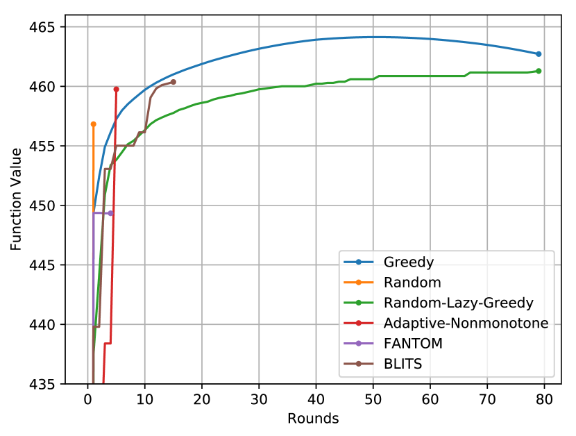
(a) Image Summarization

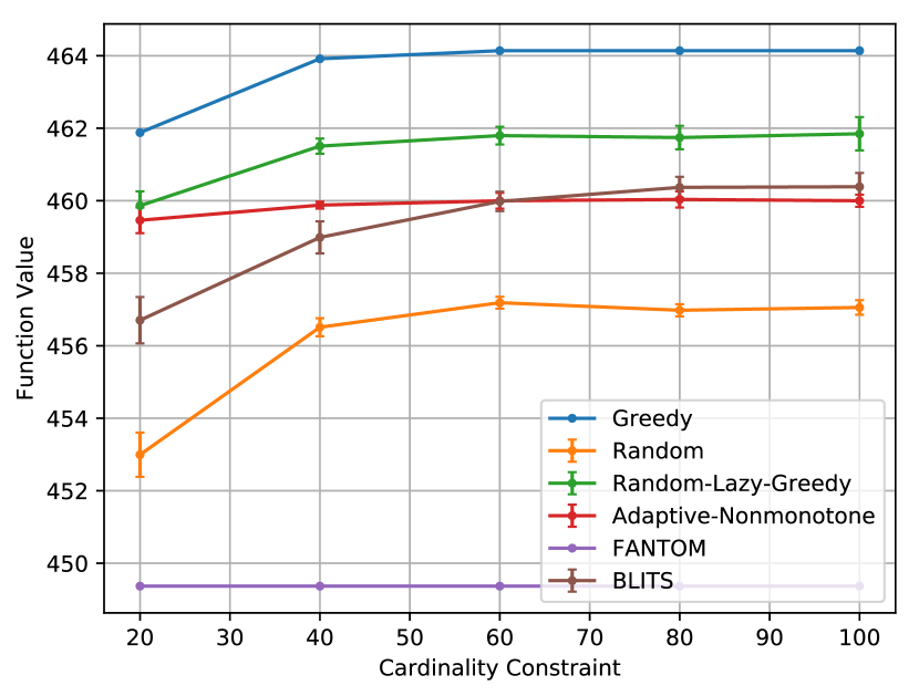
(b) Image Summarization

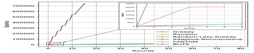
(c) Image Summarization

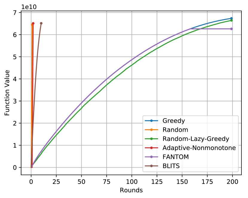
(d) Movie Recommendation

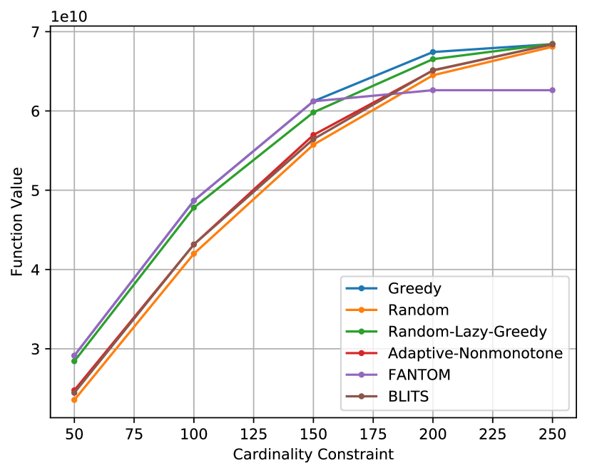
(e) Movie Recommendation

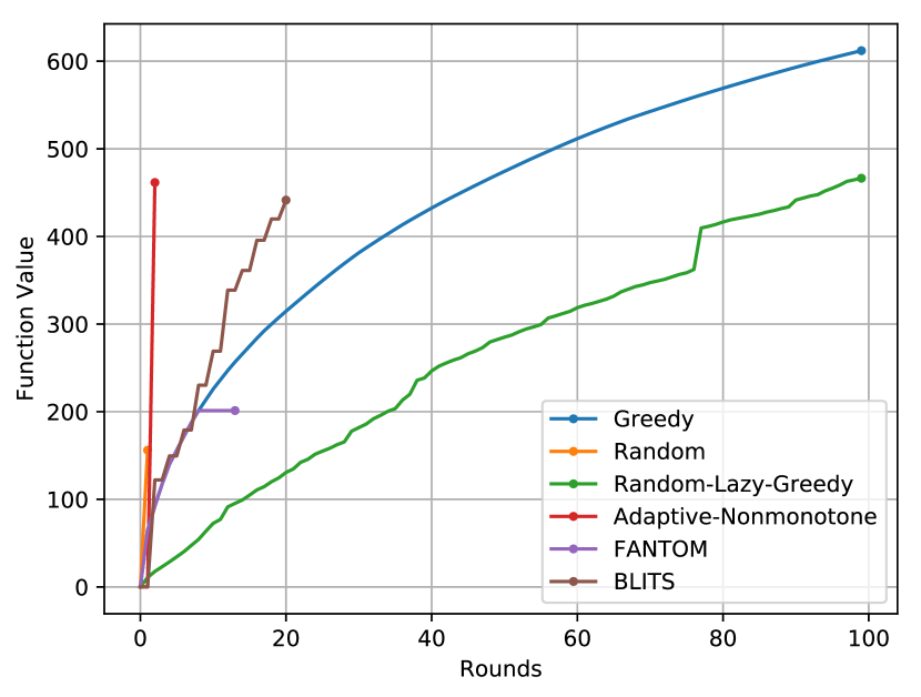
(f) Revenue Maximization

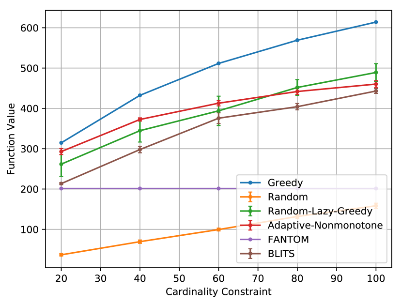
(g) Revenue Maximization

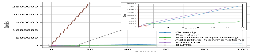
(h) Revenue Maximization

Figure 1: Performance of Adaptive-Nonmonotone-Max compared to several benchmarks for image summarization on the CIFAR-10 dataset, movie recommendation on the MovieLens 20M dataset, and revenue maximization on the top 5,000 communities of YouTube.

Image Summarization. The goal of image summarization is to find a small, representative subset from a large collection of images that accurately describes the entire dataset. The quality of a summary is typically modeled by two contrasting requirements: coverage and diversity. Coverage measures the overall representation of the dataset, and diversity encourages succinctness by penalizing summaries that contain similar images. For a collection of images $N$, the objective function we use for image summarization is

$$f(S)=\sum_{i\in N}\max_{j\in S}s_{i,j}-\frac{1}{|N|}\sum_{i\in S}\sum_{j\in S}s_{i,j},$$

where $s_{i,j}$ is the similarity between image $i$ and image $j$. The trade-off between coverage and diversity naturally gives rise to non-monotone submodular functions. We perform our image summarization experiment on the CIFAR-10 test set (Krizhevsky & Hinton, 2009), which contains 10,000 $32\times 32$ color images. The image similarity $s_{i,j}$ is measured by the cosine similarity of the 3,072-dimensional pixel vectors for images $i$ and $j$. Following Balkanski et al. (2018), we randomly select $500$ images to be our subsampled ground set since this experiment is throttled by the number and cost of oracle queries.

We set $k=80$ in Figure 1(a) and track the progress of the algorithms in each round. Figure 1(b) compares the solution quality for different constraints $k\in(20,40,60,80,100)$ and demonstrates that Adaptive-Nonmonotone-Max and Blits find substantially better solutions than Random. We use $10$ trials for each stochastic algorithm and plot the mean and standard deviation of the solutions. We note that Fantom performs noticeably worse than the others because it stops choosing elements when their (possibly positive) marginal gain falls below a fixed threshold. We give a picture-in-picture plot of the query complexities in Figure 1(c) to highlight the difference in overall cost of the estimators for Adaptive-Nonmonotone-Max and Blits.

Movie Recommendation. Personalized movie recommendation systems aim to provide short, comprehensive lists of high-quality movies for a user based on the ratings of similar users. In this experiment, we randomly sample 500 movies from the MovieLens 20M dataset (Harper & Konstan, 2016), which contains 20 million ratings for 26,744 movies by 138,493 users. We use Soft-Impute (Mazumder et al., 2010) to predict the rating vector for each movie via low-rank matrix completion, and we define the similarity of two movies $s_{i,j}$ as the inner product of the rating vectors for movies $i$ and $j$. Following Mirzasoleiman et al. (2016), we use the objective function

$$f(S)=\sum_{i\in N}\sum_{j\in S}s_{i,j}-\lambda\sum_{i\in S}\sum_{j\in S}s_{i,j},$$

with $\lambda=0.95$. Note that if $\lambda=1$ we have the cut function.

We remark that experiment is similar to solving max-cut on an Erdös-Rényi graph. In Figure 1(d) we set $k=200$, and in Figure 1(e) we consider $k\in(50,100,150,200,250)$. The Greedy algorithm performs moderately better than Random as the constraint approaches $k=250$, and all other algorithms except Fantom are sandwiched between these benchmarks. The query complexities are similar to Figure 1(c), so we exclude this plot to keep Figure 1 compact.

Revenue Maximization. In this application, our goal is to choose a subset of users in a social network to advertise a product in order to maximize its revenue. We consider the top 5,000 communities of the YouTube network (Leskovec & Krevl, 2014) and subsample the graph by restricting to 25 randomly chosen communities (Balkanski et al., 2018). The resulting network has 1,329 nodes and 3,936 edges. We assign edge weights according to the continuous uniform distribution $\mathcal{U}(0,1)$, and we measure influence using the non-monotone function

$$f(S)=\sum_{i\in N\setminus S}\sqrt{\sum_{j\in S}w_{i,j}}.$$

In Figure 1(f), we set $k=100$ and observe that Adaptive-Nonmonotone-Max significantly outperforms Fantom and Random. Figure 1(g) shows a stratification of the algorithms for $k\in(20,40,60,80,100)$, and Figure 1(h) is similar to the image summarization experiment. We note that the inner plot in Figure 1(h) shows that for the optimal threshold of Adaptive-Nonmonotone-Max, the number of candidates instantly falls below $3k$ and the algorithm outputs a random prefix of high-valued elements in the next round.

5 Conclusions

We give the first algorithm for maximizing a non-monotone submodular function subject to a cardinality constraint that achieves a constant-factor approximation with nearly optimal adaptivity complexity. The query complexity of this algorithm is also nearly optimal and considerably less than in previous works. While the approximation guarantee is only $0.039-\varepsilon$, our empirical study shows that for several real-world applications Adaptive-Nonmonotone-Max finds solutions that are competitive with benchmarks for non-monotone submodular maximization and requires significantly fewer rounds and oracle queries.

Appendix A Missing Analysis from Section 2

See 2.3

Proof.

We start by proving that the adaptivity complexity of Non-Monotone-Threshold-Sampling is $O(\log(n/\delta)/\varepsilon)$. The number of rounds is $r=O(\log_{(1-\varepsilon)^{-1}}(n/\delta))$ by construction, and there are polynomially-many queries in each round, all of which are independent and only rely on the state of $S$ at the beginning of the round. Finally, updating $S^{\prime}$ on Line 15 requires one adaptive round since each post-filtering step happens with respect to $S$ and prefixes of a fixed permutation.

Property 1.

The expected $O(n/\varepsilon)$ query complexity follows from Fahrbach et al. (2019, Lemma 3.2) for the original Threshold-Sampling algorithm since this part of their analysis holds for general submodular functions. The only change we need to consider for Non-Monotone-Threshold-Sampling is the number of queries used in the construction of $S^{\prime}$ on Line 15. For each $x_{i}\in T$, the algorithm makes two oracle calls to decide if $\Delta(x_{i},S\cup\{x_{1},\dots,x_{i-1}\})\geq\tau$, so the total query complexity of Line 15 is $2|S|=O(n)$. Therefore, the expected query complexity of the algorithm is $O(n/\varepsilon)$.

Property 2.

If $|S|<k$ when the algorithm terminates, then Non-Monotone-Threshold-Sampling did not break on Line 17. Therefore, the algorithm either (a) breaks early on Line 7, in which the property holds, or (b) finishes all $r$ rounds. In the case where all $r$ rounds finish and $|S|<k$, it follows from the proof of Fahrbach et al. (2019, Lemma 3.6) that

$$\Pr\left(|A_{r}|\geq ck\mid Z\right) \leq\Pr\left(|A_{r}|\geq 1\mid Z\right)$$

$$\leq\delta/2,$$

since we always take $c\geq 1$. Therefore, with probability at least $1-\delta/2$, the number of remaining candidates is $|A|<ck$.

Property 3.

For each round $\ell\in[r]$, let:

• $A_{\ell}$ be the value of $A$ after the filtering step in Line 6

• $T_{\ell}$ be the value of $T$

• $S_{\ell}$ be the value of $S$ before the update in Line 16

We use the round-specific values for these random sets to prove the next three properties.

Let $T_{\ell}^{\prime}\subseteq T_{\ell}$ denote the set of elements in $T_{\ell}$ that survive the post-filtering step in Line 15. We want to show that

$$\mathbb{E}\left[|T^{\prime}_{\ell}|\mid Z\right]\geq(1-\varepsilon)\mathbb{E}\left[|T_{\ell}|\mid Z\right].$$

In the for loop on Line 9, we go over iterations $i=0,1,\dots,m$. Let $t^{*}=\min\{\lfloor(1+\hat{\varepsilon})^{i}\rfloor,|A|\}$ be the final value we set for $t$ in the last iteration of the for loop on Lines 9–12. In other words, we break on Line 12 during iteration $0\leq i\leq m$, or the loop finishes. If $t^{*}=1$, then we have $|T^{\prime}_{\ell}|=|T_{\ell}|=1$ by the definition of $A_{\ell}$.

Therefore, assume that $t^{*}\geq 2$. The size $t\leq t^{*}$ in the previous iteration, where

$$t=\lfloor(1+\hat{\varepsilon})^{i-1}\rfloor\leq\lfloor(1+\hat{\varepsilon})^{i}\rfloor=t^{*},$$

satisfies $\mathbb{E}\left[I_{t}\mid Z\right]\geq 1-2\hat{\varepsilon}$ since the algorithm did not break on Line 11 in iteration $i-1$. Thus, $\mathbb{E}\left[I_{t^{\prime}}\mid Z\right]\geq 1-2\hat{\varepsilon}$ for any $0\leq t^{\prime}\leq t$. Note that we do not necessarily sample $t^{*}$ elements on Line 13 since the sample size is capped at $k-|S|$.

It follows from a decomposition of $|T^{\prime}_{\ell}|$ into indicator random variables that

$$\mathbb{E}\left[|T_{\ell}^{\prime}|\mid Z,|T_{\ell}|=b\right] =\sum_{t^{\prime}=0}^{b-1}\mathbb{E}[I_{t^{\prime}}\mid Z]$$

$$\geq\sum_{t^{\prime}=0}^{\min\{t,b-1\}}\mathbb{E}[I_{t^{\prime}}\mid Z]$$

$$\geq\left(\min\{t+1,b\}\right)(1-2\hat{\varepsilon})$$

$$\geq\frac{b}{1+\hat{\varepsilon}}(1-2\hat{\varepsilon})$$

$$\geq(1-\varepsilon)\mathbb{E}\left[|T_{\ell}|\mid Z,|T_{\ell}|=b\right].$$ (7)

To prove the second to last inequality, we get help from two observations: $t^{*}\leq(1+\hat{\varepsilon})(t+1)$, and $b\leq t^{*}$. Therefore, $\min\{t+1,b\}$ is at least $b/(1+\hat{\varepsilon})$.

Since Inequality (7) holds for any value of $|T_{\ell}|=b$, we can summarize all of them in the following form:

$$\mathbb{E}\left[|T_{\ell}^{\prime}|\mid Z\right]\geq(1-\varepsilon)\mathbb{E}\left[|T_{\ell}|\mid Z\right].$$

Putting everything together,

$$\mathbb{E}\left[|S^{\prime}|\mid Z\right] =\sum_{i=1}^{r}\mathbb{E}\left[|T_{i}^{\prime}|\mid Z\right]$$

$$\geq(1-\varepsilon)\sum_{i=1}^{r}\mathbb{E}\left[|T_{i}|\mid Z\right]$$

$$=(1-\varepsilon)\mathbb{E}\left[|S|\mid Z\right].$$

Property 4.

For each $T_{\ell}$, let the shuffled elements on Line 14 of Algorithm 1 be $(x_{\ell,1},x_{\ell,2},\dots,x_{\ell,|T_{\ell}|})$. It follows from submodularity and the definition of $S^{\prime}$ that

$$f(S^{\prime}) =\sum_{\ell=1}^{r}\sum_{j=1}^{|T_{\ell}|}\Delta(x_{\ell,j},S^{\prime}\cap(S_{\ell}\cup\{x_{\ell,1},\dots,x_{\ell,j-1}\}))\cdot\mathbf{1}_{S^{\prime}}(x_{\ell,j})$$

$$\geq\sum_{\ell=1}^{r}\sum_{j=1}^{|T_{\ell}|}\Delta(x_{\ell,j},S_{\ell}\cup\{x_{\ell,1},\dots,x_{\ell,j-1}\})\cdot\mathbf{1}_{S^{\prime}}(x_{\ell,j})$$

$$\geq\sum_{\ell=1}^{r}\sum_{j=1}^{|T_{\ell}|}\tau\cdot\mathbf{1}_{S^{\prime}}(x_{\ell,j})$$

$$=\tau\cdot|S^{\prime}|,$$

where $\mathbf{1}_{B}(x)$ is the indicator function for a set $B$ defined as $\mathbf{1}_{B}(x)=1$ if $x\in B$ and $\mathbf{1}_{B}(x)=0$ if $x\not\in B$.

Property 5.

For any $x\in N$, let $X_{\ell}$ be an indicator random variable for the event $x\in T_{\ell}$. It follows that

$$\Pr\left(x\in S\right) =\sum_{\ell=1}^{r}\mathbb{E}\left[X_{\ell}\right]\leq\sum_{\ell=1}^{r}\mathbb{E}\left[\frac{|T_{\ell}|}{|A_{\ell}|}\right]\leq\frac{1}{{\color[rgb]{0,0,0}c}k}\sum_{\ell=1}^{r}\mathbb{E}\left[|T_{\ell}|\right]=\frac{1}{{\color[rgb]{0,0,0}c}k}\mathbb{E}\left[|S|\right]\leq\frac{1}{{\color[rgb]{0,0,0}c}k}\cdot k=\frac{1}{{\color[rgb]{0,0,0}c}}.$$

We note that one can also upper bound $\Pr\left(x\in S\mid Z\right)$ as follows. If we condition on $Z$, the choices the algorithm makes in rounds $1,2,\dots,\ell$, and the size of $T_{\ell}$, then we can still upper bound the expected value of $X_{\ell}$ similarly. Summing over all possible outcomes of the algorithm and also the values of $|T_{\ell}|$ over rounds $\ell=1,2,\dots,r$, we achieve the overall upper bound of $1/c$ for $\Pr\left(x\in S\mid Z\right)$. Finally, we have

$$\Pr\left(x\in S^{\prime}\right)=\Pr\left(x\in S^{\prime}\mid x\in S\right)\Pr(x\in S)\leq\Pr(x\in S)\leq\frac{1}{{\color[rgb]{0,0,0}c}},$$

which completes the proof. ∎

See 2.6

Proof.

First assume that $\textnormal{OPT}_{A}>0$. We start by bounding the individual failure probability

$$\Pr\left(f\left(R_{i}\right)\leq(1/4-\varepsilon)\textnormal{OPT}_{A}\right)\leq\frac{3}{3+4\varepsilon}.$$

By Lemma 2.5 we have $\mathbb{E}\left[f(R_{i})\right]\geq(1/4)\textnormal{OPT}_{A}$. Using an analog of Markov’s inequality to upper bound $\mathbb{E}[f(R_{i})]$, it follows that

$$\frac{\textnormal{OPT}_{A}}{4}\leq\mathbb{E}\left[f\left(R_{i}\right)\right]\leq p\left(\frac{1}{4}-\varepsilon\right)\textnormal{OPT}_{A}+(1-p)\textnormal{OPT}_{A}.$$

Therefore, we must have $p\leq 3/(3+4\varepsilon)$. Since the subsets $R_{i}$ are chosen independently, our choice of $t$ gives us a total failure probability of

$$\Pr\left(f(S)\leq(1/4-\varepsilon)\textnormal{OPT}_{A}\right) =\prod_{i=1}^{t}\Pr\left(f(R_{i})\leq(1/4-\varepsilon)\textnormal{OPT}_{A}\right)$$

$$\leq\left(\frac{3}{3+4\varepsilon}\right)^{t}$$

$$\leq\delta.$$

This completes the proof that with probability at least $1-\delta$ we have $f(S)\geq(1/4-\varepsilon)\textnormal{OPT}_{A}$. To prove the adaptivity complexity, notice that all subsets $R_{i}$ can be generated and evaluated at once in parallel, hence the need for only one adaptive round. For the query complexity, we use the inequality $\log(1+(4/3)\varepsilon)\geq 2\varepsilon/3$, which holds for all $\varepsilon\leq 1/4$. ∎

Appendix B Missing Analysis from Section 3

See 3.3

Proof.

Fix an ordering $x_{1},x_{2},\dots,x_{|S|}$ on the elements in $S$. Expanding the expected value $\mathbb{E}[f(T)]$ and using submodularity, it follows that

$$\mathbb{E}\left[f(T)\right] =\frac{1}{\binom{|S|}{k}}\sum_{R\in{\color[rgb]{0,0,0}\binom{S}{k}}}\sum_{x_{i}\in R}\Delta\left(x_{i},\left\{x_{1},x_{2},\dots,x_{i-1}\right\}\cap R\right)$$

$$\geq\frac{1}{\binom{|S|}{k}}\sum_{R\in{\color[rgb]{0,0,0}\binom{S}{k}}}\sum_{x_{i}\in R}\Delta\left(x_{i},\left\{x_{1},x_{2},\dots,x_{i-1}\right\}\right)$$

$$=\frac{1}{\binom{|S|}{k}}\sum_{i=1}^{|S|}\binom{|S|-1}{k-1}\Delta\left(x_{i},\left\{x_{1},x_{2},\dots,x_{i-1}\right\}\right)$$

$$=\frac{k}{|S|}\cdot f(S),$$

which completes the proof. ∎

Lemma B.1.

For any sets $S,A\subseteq N$ and optimal solution $S^{*}$, if $S_{2}^{*}=S^{*}\setminus A$, then

$$f\left(S_{2}^{*}\right)-f\left(S_{2}^{*}\cup S\right)\leq f\left(S^{*}\right)-f\left(S^{*}\cup S\right).$$

Proof.

It is equivalent to show that

$$f(S_{2}^{*})+f(S^{*}\cup S)\leq f(S^{*})+f(S_{2}^{*}\cup S).$$

For any sets $X,Y\subseteq N$, we have $f(X\cap Y)+f(X\cup Y)\leq f(X)+f(Y)$ by the definition of submodularity. It follows that

$$f\left(S^{*}\cap\left(S_{2}^{*}\cup S\right)\right)+f\left(S^{*}\cup S\right)\leq f(S^{*})+f(S^{*}_{2}\cup S).$$

Therefore, it suffices to instead show that

$$f(S_{2}^{*})\leq f(S^{*}\cap(S_{2}^{*}\cup S)).$$ (8)

Let $S_{1}^{*}=S^{*}\cap A$ and write

$$S^{*}\cap\left(S_{2}^{*}\cup S\right) =\left(S^{*}\cap S_{2}^{*}\right)\cup\left(S^{*}\cap S\right)$$

$$=S_{2}^{*}\cup\left(S_{1}^{*}\cap S\right).$$

Next, fix an ordering $x_{1},x_{2},\dots,x_{\ell}$ on the elements in $S^{*}$. Summing the consecutive marginal gains of the elements in the set $S_{1}^{*}\cap S$ according to this order gives

$$f\left(S_{2}^{*}\cup\left(S_{1}^{*}\cap S\right)\right)=f(S_{2}^{*})+\sum_{x_{1},\dots,x_{\ell}\in S_{1}^{*}\cap S}\Delta\left(x_{i},S_{2}^{*}\cup\left\{x_{1},\dots,x_{i-1}\right\}\right).$$ (9)

We claim that each marginal contribution in Equation 9 is nonnegative. Assume for contradiction this is not the case. Let $x^{*}\in S_{1}^{*}\cap S$ be the first element violating this property, and let $x_{-1}^{*}$ be the previous element according to the ordering. By submodularity,

$$0>\Delta\left(x^{*},S_{2}^{*}\cup\bigcup_{x_{1},\dots,x_{-1}^{*}\in S_{1}^{*}\cap S}\left\{x_{i}\right\}\right)\geq\Delta\left(x^{*},S_{2}^{*}\cup\bigcup_{x_{1},\dots,x_{-1}^{*}\in S_{1}^{*}}\left\{x_{i}\right\}\right),$$

which implies $f(S^{*}\setminus\{x^{*}\})>f(S^{*})=\textnormal{OPT}$, a contradiction. Therefore, the inequality in Equation 8 is true, as desired. ∎

Appendix C Implementation Details from Section 4

We set $\varepsilon=0.25$ for all of the algorithms except Random-Lazy-Greedy-Improved, which we run with $\varepsilon=0.01$. Since some of the algorithms require a guess of OPT, we adjust $\varepsilon$ accordingly and fairly. We remark that all algorithms give reasonably similar results for any $\varepsilon\in[0.05,0.50]$. We set the number of queries to be $100$ for the estimators in Adaptive-Nonmonotone-Max and Blits, although for the theoretical guarantees these should be $\Theta(\log(n)/\varepsilon^{2})$ and $\Theta(\textnormal{OPT}^{2}\log(n)/\varepsilon^{2})$, respectively. For context, the experiments in Balkanski et al. (2018) set the number of samples per estimate to be 30. Last, we set the number of outer rounds for Blits to be $10$, which also matches Balkanski et al. (2018) since the number needed for provable guarantees is $r=20\log_{1+\varepsilon/2}(n)/\varepsilon$, which is too large for these datasets.

References

- Agarwal et al. (2019) Agarwal, A., Assadi, S., and Khanna, S. Stochastic submodular cover with limited adaptivity. In Proceedings of the Thirtieth Annual ACM-SIAM Symposium on Discrete Algorithms, pp. 323–342. SIAM, 2019.
- Amanatidis et al. (2021) Amanatidis, G., Fusco, F., Lazos, P., Leonardi, S., Marchetti-Spaccamela, A., and Reiffenhäuser, R. Submodular maximization subject to a knapsack constraint: Combinatorial algorithms with near-optimal adaptive complexity. In International Conference on Machine Learning, pp. 231–242. PMLR, 2021.
- Badanidiyuru et al. (2014) Badanidiyuru, A., Mirzasoleiman, B., Karbasi, A., and Krause, A. Streaming submodular maximization: Massive data summarization on the fly. In Proceedings of the 20th ACM SIGKDD International Conference on Knowledge Discovery and Data Mining, pp. 671–680. ACM, 2014.
- Balkanski & Singer (2018) Balkanski, E. and Singer, Y. The adaptive complexity of maximizing a submodular function. In Proceedings of the 50th Annual ACM SIGACT Symposium on Theory of Computing, pp. 1138–1151. ACM, 2018.
- Balkanski et al. (2018) Balkanski, E., Breuer, A., and Singer, Y. Non-monotone submodular maximization in exponentially fewer iterations. In Advances in Neural Information Processing Systems, pp. 2359–2370, 2018.
- Balkanski et al. (2019) Balkanski, E., Rubinstein, A., and Singer, Y. An exponential speedup in parallel running time for submodular maximization without loss in approximation. In Proceedings of the Thirtieth Annual ACM-SIAM Symposium on Discrete Algorithms, pp. 283–302. SIAM, 2019.
- Barbosa et al. (2015) Barbosa, R., Ene, A., Nguyen, H., and Ward, J. The power of randomization: Distributed submodular maximization on massive datasets. In International Conference on Machine Learning, pp. 1236–1244. PMLR, 2015.
- Barbosa et al. (2016) Barbosa, R. d. P., Ene, A., Nguyen, H. L., and Ward, J. A new framework for distributed submodular maximization. In 2016 IEEE 57th Annual Symposium on Foundations of Computer Science (FOCS), pp. 645–654. IEEE, 2016.
- Buchbinder & Feldman (2019) Buchbinder, N. and Feldman, M. Constrained submodular maximization via a nonsymmetric technique. Mathematics of Operations Research, 44(3):988–1005, 2019.
- Buchbinder et al. (2014) Buchbinder, N., Feldman, M., Naor, J. S., and Schwartz, R. Submodular maximization with cardinality constraints. In Proceedings of the Twenty-Fifth Annual ACM-SIAM Symposium on Discrete Algorithms, pp. 1433–1452. SIAM, 2014.
- Buchbinder et al. (2016) Buchbinder, N., Feldman, M., and Schwartz, R. Comparing apples and oranges: Query trade-off in submodular maximization. Mathematics of Operations Research, 42(2):308–329, 2016.
- Chekuri & Quanrud (2019a) Chekuri, C. and Quanrud, K. Parallelizing greedy for submodular set function maximization in matroids and beyond. In Proceedings of the 51st Annual ACM SIGACT Symposium on Theory of Computing, pp. 78–89. ACM, 2019a.
- Chekuri & Quanrud (2019b) Chekuri, C. and Quanrud, K. Submodular function maximization in parallel via the multilinear relaxation. In Proceedings of the Thirtieth Annual ACM-SIAM Symposium on Discrete Algorithms, pp. 303–322. SIAM, 2019b.
- Chen et al. (2019) Chen, L., Feldman, M., and Karbasi, A. Unconstrained submodular maximization with constant adaptive complexity. In Proceedings of the 51st Annual ACM SIGACT Symposium on Theory of Computing, pp. 102–113. ACM, 2019.
- Chen & Kuhnle (2022) Chen, Y. and Kuhnle, A. Practical and parallelizable algorithms for non-monotone submodular maximization with size constraint. arXiv preprint arXiv:2009.01947, 2022.
- Das & Kempe (2008) Das, A. and Kempe, D. Algorithms for subset selection in linear regression. In Proceedings of the Fortieth Annual ACM Symposium on Theory of Computing, pp. 45–54. ACM, 2008.
- Dueck & Frey (2007) Dueck, D. and Frey, B. J. Non-metric affinity propagation for unsupervised image categorization. In Computer Vision, 2007. ICCV 2007. IEEE 11th International Conference on, pp. 1–8. IEEE, 2007.
- El-Arini & Guestrin (2011) El-Arini, K. and Guestrin, C. Beyond keyword search: Discovering relevant scientific literature. In Proceedings of the 17th ACM SIGKDD International Conference on Knowledge Discovery and Data Mining, pp. 439–447. ACM, 2011.
- Elenberg et al. (2018) Elenberg, E. R., Khanna, R., Dimakis, A. G., and Negahban, S. Restricted strong convexity implies weak submodularity. The Annals of Statistics, 46(6B):3539–3568, 2018.
- Ene & Nguyen (2019) Ene, A. and Nguyen, H. L. Submodular maximization with nearly-optimal approximation and adaptivity in nearly-linear time. In Proceedings of the Thirtieth Annual ACM-SIAM Symposium on Discrete Algorithms, pp. 274–282. SIAM, 2019.
- Ene et al. (2018) Ene, A., Nguyen, H. L., and Vladu, A. A parallel double greedy algorithm for submodular maximization. arXiv preprint arXiv:1812.01591, 2018.
- Ene et al. (2019) Ene, A., Nguyen, H. L., and Vladu, A. Submodular maximization with matroid and packing constraints in parallel. In Proceedings of the 51st annual ACM SIGACT Symposium on Theory of Computing, pp. 90–101. ACM, 2019.
- Fahrbach et al. (2019) Fahrbach, M., Mirrokni, V., and Zadimoghaddam, M. Submodular maximization with nearly optimal approximation, adaptivity and query complexity. In Proceedings of the Thirtieth Annual ACM-SIAM Symposium on Discrete Algorithms, pp. 255–273. SIAM, 2019.
- Feige et al. (2011) Feige, U., Mirrokni, V. S., and Vondrak, J. Maximizing non-monotone submodular functions. SIAM Journal on Computing, 40(4):1133–1153, 2011.
- Gharan & Vondrák (2011) Gharan, S. O. and Vondrák, J. Submodular maximization by simulated annealing. In Proceedings of the Twenty-Second Annual ACM-SIAM Symposium on Discrete Algorithms, pp. 1098–1116. SIAM, 2011.
- Harper & Konstan (2016) Harper, F. M. and Konstan, J. A. The movielens datasets: History and context. ACM Transactions on Interactive Intelligent Systems (TIIS), 5(4):19, 2016.
- Hartline et al. (2008) Hartline, J., Mirrokni, V., and Sundararajan, M. Optimal marketing strategies over social networks. In Proceedings of the 17th international conference on World Wide Web, pp. 189–198. ACM, 2008.
- Kazemi et al. (2018) Kazemi, E., Zadimoghaddam, M., and Karbasi, A. Scalable deletion-robust submodular maximization: Data summarization with privacy and fairness constraints. In International Conference on Machine Learning, pp. 2549–2558. PMLR, 2018.
- Khanna et al. (2017) Khanna, R., Elenberg, E. R., Dimakis, A. G., Negahban, S., and Ghosh, J. Scalable greedy feature selection via weak submodularity. In Proceedings of the 20th International Conference on Artificial Intelligence and Statistics, pp. 1560–1568, 2017.
- Krizhevsky & Hinton (2009) Krizhevsky, A. and Hinton, G. Learning multiple layers of features from tiny images. Technical report, Citeseer, 2009.
- Kuhnle (2021) Kuhnle, A. Nearly linear-time, parallelizable algorithms for non-monotone submodular maximization. In Proceedings of the AAAI Conference on Artificial Intelligence, volume 35, pp. 8200–8208, 2021.
- Kumar et al. (2015) Kumar, R., Moseley, B., Vassilvitskii, S., and Vattani, A. Fast greedy algorithms in mapreduce and streaming. ACM Transactions on Parallel Computing (TOPC), 2(3):14, 2015.
- Lattanzi et al. (2011) Lattanzi, S., Moseley, B., Suri, S., and Vassilvitskii, S. Filtering: A method for solving graph problems in mapreduce. In Proceedings of the Twenty-Third Annual ACM Symposium on Parallelism in Algorithms and Architectures, pp. 85–94. ACM, 2011.
- Lee et al. (2010) Lee, J., Mirrokni, V. S., Nagarajan, V., and Sviridenko, M. Maximizing nonmonotone submodular functions under matroid or knapsack constraints. SIAM Journal on Discrete Mathematics, 23(4):2053–2078, 2010.
- Leskovec & Krevl (2014) Leskovec, J. and Krevl, A. SNAP Datasets: Stanford large network dataset collection. http://snap.stanford.edu/data, June 2014.
- Liu & Vondrák (2019) Liu, P. and Vondrák, J. Submodular optimization in the MapReduce model. In 2nd Symposium on Simplicity in Algorithms, volume 69, pp. 18:1–18:10. Schloss Dagstuhl - Leibniz-Zentrum für Informatik, 2019.
- Mazumder et al. (2010) Mazumder, R., Hastie, T., and Tibshirani, R. Spectral regularization algorithms for learning large incomplete matrices. Journal of Machine Learning Research, 11:2287–2322, 2010.
- Mirrokni & Zadimoghaddam (2015) Mirrokni, V. and Zadimoghaddam, M. Randomized composable core-sets for distributed submodular maximization. In Proceedings of the Forty-Seventh Annual ACM Symposium on Theory of Computing, pp. 153–162. ACM, 2015.
- Mirzasoleiman et al. (2013) Mirzasoleiman, B., Karbasi, A., Sarkar, R., and Krause, A. Distributed submodular maximization: Identifying representative elements in massive data. In Advances in Neural Information Processing Systems, pp. 2049–2057, 2013.
- Mirzasoleiman et al. (2016) Mirzasoleiman, B., Badanidiyuru, A., and Karbasi, A. Fast constrained submodular maximization: Personalized data summarization. In International Conference on Machine Learning, pp. 1358–1367. PMLR, 2016.
- Mohri et al. (2018) Mohri, M., Rostamizadeh, A., and Talwalkar, A. Foundations of Machine Learning. MIT Press, 2018.
- Nemhauser et al. (1978) Nemhauser, G. L., Wolsey, L. A., and Fisher, M. L. An analysis of approximations for maximizing submodular set functions. Mathematical Programming, 14(1):265–294, 1978.
- Norouzi-Fard et al. (2018) Norouzi-Fard, A., Tarnawski, J., Mitrovic, S., Zandieh, A., Mousavifar, A., and Svensson, O. Beyond 1/2-approximation for submodular maximization on massive data streams. In International Conference on Machine Learning, pp. 3829–3838. PMLR, 2018.
- Qian & Singer (2019) Qian, S. and Singer, Y. Fast parallel algorithms for statistical subset selection problems. In Advances in Neural Information Processing Systems, volume 32, 2019.
- Simon et al. (2007) Simon, I., Snavely, N., and Seitz, S. M. Scene summarization for online image collections. In 2007 IEEE 11th International Conference on Computer Vision, pp. 1–8. IEEE, 2007.
- Sipos et al. (2012) Sipos, R., Swaminathan, A., Shivaswamy, P., and Joachims, T. Temporal corpus summarization using submodular word coverage. In Proceedings of the 21st ACM International Conference on Information and Knowledge Management, pp. 754–763. ACM, 2012.
- Tschiatschek et al. (2014) Tschiatschek, S., Iyer, R. K., Wei, H., and Bilmes, J. A. Learning mixtures of submodular functions for image collection summarization. In Advances in Neural Information Processing Systems, pp. 1413–1421, 2014.