The double population of Chamaeleon I detected by Gaia DR2

Abstract

Context. Chamaeleon I represents an ideal laboratory to study the cluster formation in a low-mass environment. Recently, two sub-clusters spatially located in the northern and southern parts of Chamaeleon I were found with different ages and radial velocities.

Aims. In this letter we report new insights into the structural properties, age, and distance of Chamaeleon I based on the astrometric parameters from Gaia data-release 2 (DR2).

Methods. We identified 140 sources with a reliable counterpart in the Gaia DR2 archive. We determined the median distance of the cluster using Gaia parallaxes and fitted the distribution of parallaxes and proper motions assuming the presence of two clusters. We derived the probability of each single source of belonging to the northern or southern sub-clusters, and compared the HR diagram of the most probable members to pre-main sequences isochrones.

Results. The median distance of Chamaeleon I is $\sim$190 pc. This is about 20 pc larger than the value commonly adopted in the literature. From a Kolmogorov-Smirnov test of the parallaxes and proper-motion distributions we conclude that the northern and southern clusters do not belong to the same parent population. The northern population has a distance d_N = 192.7${}^{+0.4}_{-0.4}$ pc, while the southern one d_S = 186.5${}^{+0.7}_{-0.7}$ pc. The two sub-clusters appear coeval, at variance with literature results, and most of the sources are younger than 3 Myr. The northern cluster is more elongated and extends towards the southern direction partially overlapping with the more compact cluster located in the south. A hint of a relative rotation between the two sub-clusters is also found.

1 Introduction

Chamaeleon I is one of the closest low-mass star forming regions with which it is possible to study all the key processes related to the formation of a young cluster, as well as the structure of protoplanetary disks around young stellar objects.
The stellar population of Chamaeleon I has been extensively investigated in the last fifteen years (Feigelson & Lawson 2004; Stelzer et al. 2004; Comerón et al. 2004). The cluster is composed of two sub-structures, one northern and one southern. A complete study was presented by Luhman (2007) who found the two populations to have different ages: 5-6 Myr for the northern and 3-4 Myr for the southern sub-cluster, respectively. The structure and dynamical properties of Chamaeleon I have been deeply investigated by Sacco et al. (2017), who confirmed the presence of the two sub-clusters kinematically, with a shift in velocity of about 1 km/s.

The literature value of the distance of Chamaeleon I commonly adopted is 160 $\pm$ 15 pc (Whittet et al. 1997). This value comes from the combination of studies that employed different techniques. In particular, the extinction analysis of Whittet et al. (1997) constrained the distance in the range between 135 and 165 pc, while the weighted average of Hipparcos distances for three cluster members , is 175${}^{+20}_{-16}$ pc (Perryman et al. 1997).
Gaia DR2 astrometry (Gaia Collaboration et al. 2018; Lindegren et al. 2018) clearly offers a unique opportunity to gather a new view of the region.

In this letter we present the parallaxes and proper motions of the cluster members spectroscopically identified by previous works. The analysis of the Gaia DR2 data and the discussion of the clusters kinematics and age are in Sects. 3 and 4, respectively.

2 Cluster membership and Gaia DR2 data

Our approach aims to characterize the previously known populations rather than to discover possible new members of the region. For this reason, we compiled a catalog of 244 optical members, combining the observations of Luhman (2007) and Sacco et al. (2017). From this initial catalog, 206 sources are present in the Gaia DR2 archive, but for any further analysis we consider only the 140 with an excess source noise less than 1 (as suggested e.g., in Lindegren et al. 2018). All details oft the relations between astrometric excess noise and parallax are given in Appendix A.
Assuming that all the cluster members belong to the same population, it is possible to compute the distance of the entire cluster. Figure 1 shows the distribution of the parallaxes of the cluster members; the distance commonly adopted in the literature for Chamaeleon I is highlighted.
The resulting median parallax is 5.248$\pm$0.187 mas, where the associated error is computed as the median absolute deviation (MAD). Since the relative error is lower than 10$\%$, we can calculate the distance by inverting the parallax (Luri et al. 2018; Bailer-Jones 2015). The distance of Chamaeleon I is therefore 190.5${}^{+7.1+3.8}_{-6.5-3.5}$ pc, which takes into account a conservative systematic error of 0.1 mas, as discussed by Luri et al. (2018). This distance is larger than previously assumed in the literature (Whittet et al. 1997), while being marginally consistent with the Hipparcos distance from three members only.

The spatial distribution of the cluster members (after a 3-sigma clipping on the initial sample) is plotted as a function of the parallaxes and proper motions in Fig. 2. The two sub-clusters spatially identified by Luhman (2007) can be clearly distinguished in parallax and kinematically.

3 Analysis

In order to quantitatively investigate whether the two sub-clusters are also separated in parallax and kinematics, we selected the northern and southern regions using the criterium of Luhman (2007) based on their declinations; lower than -77^∘ for the northern sub-cluster, and higher than -77^∘ for the southern one. We performed a two-sample Kolmogorov-Smirnov test in parallaxes and proper motions. The probabilities that the two samples belong to the same parent population are 2.39$\,\cdot\,10^{-12}$, 8.0$\,\cdot\,10^{-14}$ and 1.84$\,\cdot\,10^{-11}$ in parallax, proper motion in $\alpha$ and $\delta$, respectively. This confirms statistically that the two clusters are spatially separated in parallax and kinematically separated in proper motions.

We fitted the distribution of the three astrometric parameters ($\pi_{i}$, $\mu_{\alpha,i}$, and $\mu_{\delta,i}$) with a model including two populations, described by two three-dimensional (3D) multivariate Gaussians (as in Lindegren et al. 2000, ). To perform our calculations, we used a maximum likelihood approach as in Jeffries et al. (2014) and Franciosini et al. (2018).

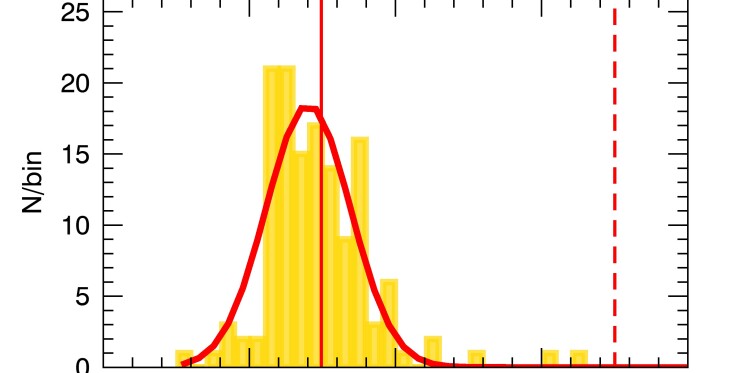
Figure 1: Histogram of the parallaxes of the Chamaeleon I members. The solid red line represents the position of the median parallax. The dotted red vertical line represents the parallax commonly adopted from the literature. The result of a Gaussian fit is also shown.

The likelihood function for each star of each population is given by

$$\vskip 3.0pt plus 1.0pt minus 1.0ptL_{N/S,i}=(2\pi)^{-3/2}\,|C_{i}|^{-1/2}\times\exp{\begin{bmatrix}-\frac{1}{2}(a_{i}-a_{0})^{\prime}\,C_{i}^{-1}\,(a_{i}-a_{0})\end{bmatrix}},$$ (1)

where $C_{i}$ is the covariance matrix, $|C_{i}|$ its determinant (the details on each term of the matrix are given in Appendix B), and
$(a_{i}-a_{0})^{\prime}$ is the transpose of the vector

$$a_{i}-a_{0}=\begin{bmatrix}\pi_{i}-\pi_{0}\\ \mu_{\alpha,i}-\mu_{\alpha,0}\\ \mu_{\delta,i}-\mu_{\delta,0}\end{bmatrix},$$ (2)

where $\pi_{0}$, $\mu_{\alpha,0}$, $\mu_{\delta,0}$ are the mean values of the cluster.
The total likelihood of the double population is therefore given by:

$$L_{i}=f_{N}\,L_{N,i}\,+\,(1-f_{N})\,L_{S,i},$$ (3)

where $L_{N}$ and $L_{S}$ are the likelihoods given in Equation 1 for the northern and southern sub-clusters, $f_{N}$ is the fraction of stars that belongs to the north component, and $f_{S}\,=\,(1-f_{N})$ is the fraction of southern stars. This is a reliable assumption for this region since our membership is based on different accurate studies. We warn the reader that in other fields with higher contaminations this assumption cannot be applied since it excludes the possibility of having interlopers or any type of contamination by non-members of either of the clusters.

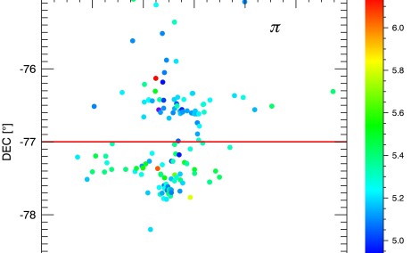
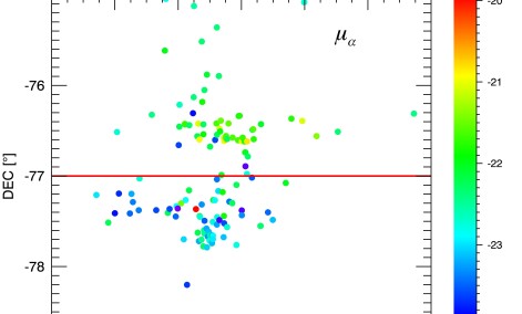
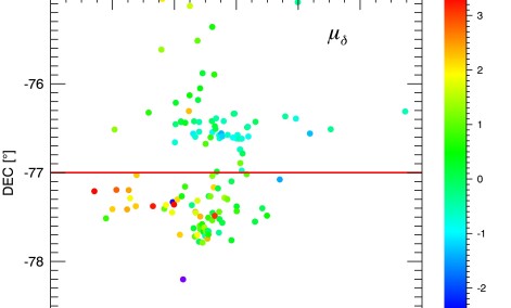
Figure 2: Spatial distribution of sources color coded by parallaxes and proper motions. The horizontal red lines highlight the declination of -77^∘ used by Luhman (2007) to distinguish the two sub-clusters.

The probability for each star of belonging to either the sub-cluster N or S is computed as

$$\begin{array}[]{rl}\vskip 3.0pt plus 1.0pt minus 1.0ptP_{N,i}\,=\,f_{N}\frac{L_{N,i}}{L_{i}}&P_{S,i}\,=\,(1-f_{N})\frac{L_{S,i}}{L_{i}}\end{array}.$$ (4)

Table 1: Results from the MLE fit of the two sub-clusters of Chamaeleon I: parallax with its error ($\pi$), the parallax dispersion and its error $\sigma_{\pi,0}$ , the proper motions $\mu_{\alpha}$ and $\mu_{\delta}$ with their errors and the relative dispersions $\sigma_{\mu_{\alpha},0}$ $\sigma_{\mu_{\delta,0}}$ with their errors. The definition of the dispersions in parallax and proper motions is given in Appendix B.

	$\pi$	$\sigma_{\pi,0}$	$\mu_{\alpha}$	$\sigma_{\mu_{\alpha},0}$	$\mu_{\delta}$	$\sigma_{\mu_{\delta,0}}$
Cha I North	5.188$\pm$0.012	0.060$\pm$0.011	-22.069$\pm$0.101	0.738$\pm$0.063	-0.050$\pm$0.115	0.873$\pm$0.079
Cha I South	5.363$\pm$0.021	0.085$\pm$0.017	-23.127$\pm$0.114	0.571$\pm$0.072	1.593$\pm$0.238	1.126$\pm$0.159
frac N	0.638$\pm$0.068
ln($L$)max	-271.69

Out of the initial 140 sources, we found that 107 have a probability higher than 80$\%$ of belonging to one of the two sub-clusters. The results are listed in Table 1.
We highlight that the uncertainties in parallax and proper motions considered in the analysis include only the published errors provided in the Gaia DR2 archive, which are derived from the formal error in the astrometric processing. Since a simple receipt to account for systematic error is not yet available, Luri et al. (2018) suggested to discuss a possible influence on the scientific results of a systematic error not larger than 0.1 mas in parallax and 0.1 mas/yr for proper motions. We highlight that there is no reason to expect a different systematic error between the two clusters, since they are located in the same direction on the sky and are composed of a homogenous sample of stars in spectral types and magnitudes. For these reasons the systematic errors do not introduce any effect to our results.
Inverting the parallaxes, we can derive the distances of the two sub-clusters:

d_N = 192.7${}^{+0.4}_{-0.4}$ pc               d_S = 186.5${}^{+0.7}_{-0.7}$ pc.

In Figure 3 we show the histograms of the parallax distribution of the 73 most probable northern members, and the 34 southern members, where we have highlighted the parallaxes of the two sub-clusters computed from the maximum likelihood estimation (MLE), as well as their spatial distribution. The projected distance between the centers of both clusters along the line of sight is of the same order as their projected separation in the plane of the sky and as their spatial extent. This supports the hypothesis that they both belong to the same physical entity, and it is not only a chance alignment along the line of sight. We see that the southern cluster has a compact structure, while the northern cluster, which corresponds to the more distant one, is spatially more elongated and extends in the direction of the southern cluster.

This may reflect the influence of the main filamentary structure present in the region, which extends in the north-south direction and has been mapped in C¹⁸O by Haikala et al. (2005).

4 Discussion and Conclusion

In this section we discuss the age and the kinematic properties of the north and south sub-clusters of Chamaeleon I.

4.1 The age of Chamaeleon I

In order to investigate whether an age difference is present between the two sub-clusters, we consider the 107 members with a probability higher than 80$\%$ defined in Section 3. We use the log(T_eff)-M_J diagram in order to minimize the effects due to infrared excesses caused by the presence of protostellar disks. The effective temperatures are compiled either from Luhman (2007) or from Sacco et al. (2017). The absolute J magnitude of each source has been derived by adopting the mean distance module for the northern and southern sub-clusters and correcting for $A_{J}$ (from Luhman 2007). The overplotted isochrones are the Z=0.013 models from Tognelli et al. (2011) . These models have a solar metallicity, which is a good approximation for the metallicity of the cluster as found by Spina et al. (2017).
As shown in Figure 4, all the sources have ages lower than 5 Myr. In particular, apart for a few sources, most of the members are younger than 3 Myr. While Luhman (2007) found different ages for the two populations (5-6 Myr for the northern one and 3-4 Myr for the southern one), we do not find any evidence of an age difference between the two sub-clusters.
Our new findings and the differences with respect to the Luhman (2007) results can be ascribed to two effects: on one hand, Luhman (2007) used the same distance to all sources, adopting a smaller value than what we find here; on the other hand, his selection of the two sub-clusters was based only on the spatial distribution, while in our case we take into account also their different parallaxes and kinematic properties.

4.2 Kinematics properties of the north and south sub-clusters

Under the assumption of an isotropic distribution in a star cluster, we can use the relation of Platais (2012) to derive the velocity dispersion from the proper motion dispersion:

$$\sigma_{r}(km/s)=d\,(kpc)\,\cdot\,4.37\,\cdot\,\sigma_{\mu}(mas/yr),$$ (5)

where the $\sigma_{\mu}^{2}=\frac{\sigma_{\mu_{\alpha}}^{2}+\sigma_{\mu_{\delta}}^{2}}{2}$ (McLaughlin et al. 2006).
We obtain $\sigma_{r,N}=0.681\pm 0.057$ km/s and $\sigma_{r,S}=0.727\pm 0.134$ km/s, where the uncertainties are computed from the error propagation. The velocity dispersions are consistent, within 2 $\sigma$, with the results of Sacco et al. (2017).

Given that the northern cluster is in the background, and it is more redshifted than the closer southern sub-cluster, we conclude that the two clusters are moving away from each other.

In Figure 3 the two arrows represent the proper motions of the two sub-clusters with respect to a reference system centered on the cluster. This confirms that the two sub-clusters are not merging and have a non-zero angular momentum. Combining this result with the differential radial velocity measured by Sacco et al. (2017), this represents a hint of rotation of the two sub-clusters. This is a new and puzzling result. Indeed, in young high-mass clusters rotation has been theoretically predicted by Mapelli (2017), and it has been observed, for example, in the high-mass star forming region R136 in the Large Magellanic Cloud (Hénault-Brunet et al. 2012). However, in simulations with similar total mass to low-mass environments, such as Chamaeleon I, Mapelli (2017) did not find a clear signature of rotation as in high-mass environments.

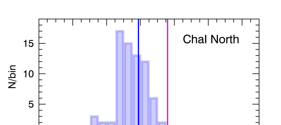
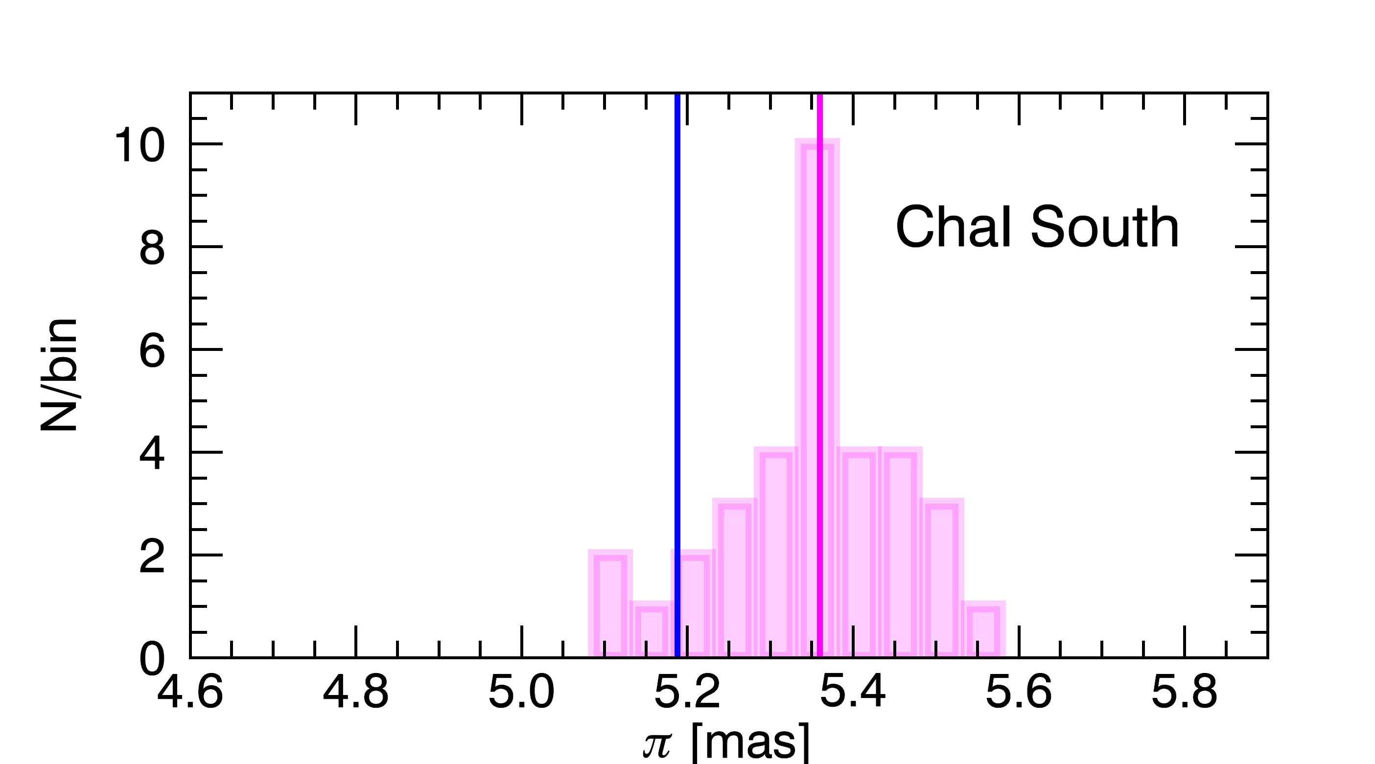
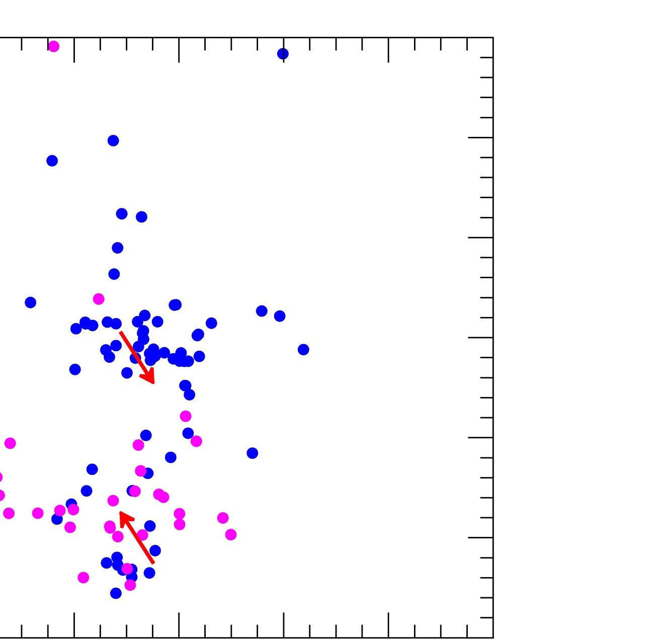
Figure 3: Left: Parallax distribution of the most probable members (P$\geq$80$\%$) of the northern (in blue) and southern (in magenta) sub-clusters. In each panel the MLE parallaxes for both clusters are shown. Right: Spatial distribution of the northern and the southern sub-cluster (as in the left panel). The red arrows represent the differential proper motions in $\alpha$ and $\delta$ with respect to a mean proper motion between the northern and southern cluster.

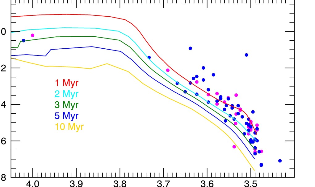
Figure 4: log(T_eff) - M_J Diagram of the most probable members (P$\geq$80$\%$). The color code is as in Figure 3. The solid lines are the pre-main sequence isochrones at different ages between 1 and 10 Myr. .

A more detailed analysis of the cluster dynamics will be presented in an upcoming paper, together with an updated census of the members using Gaia DR2 data.

Appendix A Selection data

In this appendix we show the distribution of all the parallaxes and parallax errors of the 206 sources with a Gaia counterpart. In the last lower panel we see the effect of selecting only the sources with excess errors lower than 1, and we notice that in this way almost all the sources with higher error in parallax are automatically excluded from our analysis.

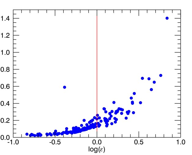
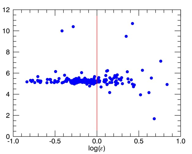
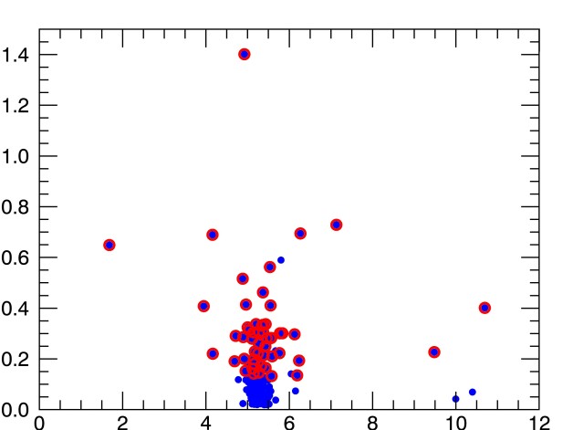
Figure 5: Upper two panels: distribution of the parallaxes and errors in parallax as a function of the astrometric excess noise. The vertical red line corresponds to the excess noise = 1. Bottom panel: parallaxes vs. the error in parallaxes. Sources excluded by our analysis are highlighted with red circles.

Appendix B Probability density function

The covariance matrix $C_{i}$ of Equation 1 corresponds to

$$C_{i}=\begin{bmatrix}C_{i,11}&C_{i,12}&C_{i,13}\\ C_{i,21}&C_{i,22}&C_{i,23}\\ C_{i,31}&C_{i,32}&C_{i,33}\end{bmatrix}.$$ (6)

Following Lindegren et al. (2000) each term of the covariance matrix corresponds to:

$$\begin{array}[]{rcl}\vskip 3.0pt plus 1.0pt minus 1.0pt\begin{bmatrix}C_{i}\end{bmatrix}_{11}&=&\sigma_{\pi,i}^{2}+\sigma_{\pi,0}^{2}\\ \vskip 3.0pt plus 1.0pt minus 1.0pt\begin{bmatrix}C_{i}\end{bmatrix}_{22}&=&\sigma_{\mu_{\alpha,i}}^{2}+\sigma_{\mu_{\alpha,0}}^{2}\\ \vskip 3.0pt plus 1.0pt minus 1.0pt\begin{bmatrix}C_{i}\end{bmatrix}_{33}&=&\sigma_{\mu_{\delta,i}}^{2}+\sigma_{\mu_{\delta,0}}^{2}\\ \vskip 3.0pt plus 1.0pt minus 1.0pt\begin{bmatrix}C_{i}\end{bmatrix}_{12}&=&\begin{bmatrix}C_{i}\end{bmatrix}_{21}=\sigma_{\pi,i}\cdot\sigma_{\mu_{\alpha,i}}\cdot\rho\,(\pi,\mu_{\alpha})\\ \vskip 3.0pt plus 1.0pt minus 1.0pt\begin{bmatrix}C_{i}\end{bmatrix}_{13}&=&\begin{bmatrix}C_{i}\end{bmatrix}_{31}=\sigma_{\pi,i}\cdot\sigma_{\mu_{\delta,i}}\cdot\rho\,(\pi,\mu_{\delta})\\ \vskip 3.0pt plus 1.0pt minus 1.0pt\begin{bmatrix}C_{i}\end{bmatrix}_{23}&=&\begin{bmatrix}C_{i}\end{bmatrix}_{32}=\sigma_{\mu_{\alpha,i}}\cdot\sigma_{\mu_{\delta,i}}\cdot\rho\,(\mu_{\alpha},\mu_{\delta}),\\ \end{array}$$ (7)

where $\rho\,(\pi,\mu_{\alpha})$, $\rho\,(\pi,\mu_{\delta})$, $\rho\,(\mu_{\alpha},\mu_{\alpha})$ are the correlation coefficients, $\sigma_{\pi,i}$, $\sigma_{\mu_{\alpha,i}}$ and $\sigma_{\mu_{\delta,i}}$ are the errors associated to each measurement², while $\sigma_{\pi,0}$, $\sigma_{\mu_{\alpha,0}}$ and $\sigma_{\mu_{\delta,0}}$ are the intrinsic dispersions of $\pi$, $\mu_{\alpha}$ and $\mu_{\delta}$ obtained from the Maximum Likelihood Estimation of the probability given in Eqs. 3 and 1.