Abstract

Many aspects of the evolution of stars, and in particular the evolution of binary stars, remain beyond our ability to model them in detail. Instead, we rely on observations to guide our often phenomenological models and pin down uncertain model parameters. To do this statistically requires population synthesis. Populations of stars modelled on computers are compared to populations of stars observed with our best telescopes. The closest match between observations and models provides insight into unknown model parameters and hence the underlying astrophysics. In this brief review, we describe the impact that modern big-data surveys will have on population synthesis, the large parameter space problem that is rife for the application of modern data science algorithms, and some examples of how population synthesis is relevant to modern astrophysics.

Reprinted from The Impact of Binaries on Stellar Evolution, Beccari G. & Boffin H.M.J. (Eds.), © 2018 Cambridge University Press.

Chapter 0 Population synthesis of binary stars

Robert G. Izzard

Ghina M. Halabi

1 Introduction

The evolution of binary stars is often quite different to their solitary cousins (De Marco and Izzard,, 2017). Many types of stars only form in binaries, and their properties allow investigation into astrophysics that is impossible to probe in single stars. Good examples include type Ia supernovae, merging neutron stars (kilonovae) and black holes, the most massive stars e.g. blue stragglers, many massive Wolf-Rayet stars, X-ray binaries, long and short gamma-ray bursts, barium/CH/CEMP-s stars, Algols with peculiar surface chemistry for their evolutionary state, W Uma contact binaries, low-mass helium stars and related sdB and sdO stars, sequence D variable stars, and thermonuclear novae. Other processes in which binaries are implicated include the formation of asymmetric planetary nebulae, many post-(asyptotic-)giant-branch stars with circumbinary discs and overmassive stars in the Galactic thick disc. Triple and higher-multiple systems are often hierarchical, e.g. triples are effectively a long-period outer binary system containing a short-period inner binary.

Many aspects of binary-star physics remain highly uncertain. Mass transfer, accretion and loss, and associated angular momentum redistribution, e.g. common envelope evolution, dominates our ignorance of binary-star evolution. One way to improve our knowledge is to apply statistical techniques to compare our stellar models to the stars we observe. This process is called stellar population synthesis. In this brief review, we consider the challenge and opportunity that big data from modern astronomy brings, the basic technique of binary star population synthesis, and the associated parameter space problem. As an example of binary population synthesis we consider how the chemical ejecta from stars depend on model input parameters. We also show an example of how modelling metal-poor stars led to better astrophysical understanding. Finally, we report on recent population synthesis work, in particular with respect to predicting and understanding the discovery of gravitational waves from stellar and black-hole mergers.

2 Big Data and Big Challenges

The age of big data is very much upon us. From commerce to industry to pure blue-skies research, the volume of data continues to increase endlessly. Astronomy is no exception. The Gaia satellite is currently monitoring more than a billion stars with trillions of observations. Transient surveys, such as Pan-STARRS, Skymapper and the upcoming LSST, monitor billions of objects in the night sky to detect stellar explosions. Such large numbers are difficult to comprehend on a human level. Even the human population of Earth, currently in excess of $7\times 10^{9}$, is difficult to imagine. To modern, massively parallel computers, the challenge is rather less daunting. Commercial companies, especially in the financial sector, process such data daily. There are thus natural links to astrophysics, where the challenge is to understand the stars and galaxies we see, both individually and as a collective. This is where population synthesis modelling is such a useful tool. The general idea is to simulate a population of stars on a computer, and compare simulated observables to those we see. By varying the input parameters of the population model to match the stars that are seen, we can pin down the underlying astrophysics. Often, new physics can be ruled out because the numbers fail to match, and uncertain physics can be far better constrained.

Population synthesis is particularly useful because astrophysics is mostly not an experimental science. We want to answer fundamental questions, such as how do stars function, how did they get there and what are they going to do in the future. But we cannot – yet! – experiment on stars. This is analogous to a dendrologist examining the trees of a forest. Some are small, some are large, some are green and some yellow, some are in flower and some are dead. From this snapshot in time the dendrologist must determine the entire biology and evolutionary history of trees: a difficult task! Astronomers have been trying to do this for millennia with the stars in the sky. Although we cannot experiment on stars directly, through population synthesis we can experiment inside our computers and statistically compare to our forest of stars.

First, we make a set of models of stars to attempt to match those under investigation. Quantitative computer models of stars have been constructed for at least fifty years. The current state of the art is to combine one-dimensional stellar structure equations with parametrised models of internal mixing and rotational deformation. Despite these simplifications, such computer codes take hours to compute the evolution of a single star from birth to death, even when details such as thermal pulses and supernovae are ignored. Assuming the evolution can be calculated, the second step is to turn such models into a stellar population. For this, we need a description of the population’s initial parameters such as an initial mass function. Next, we must convert the models into simulated observations. This is rarely a trivial task. Stellar models predict physical parameters such as luminosity, effective temperature and chemical abundances. Observations are of usually of stellar apparent magnitudes, colours and spectral line widths, so conversion is required. Survey selection biases must be taken into account when making the simulated population. If such biases are simple – say, a luminosity cut off – then this is relatively easy. In general, biases are poorly known and sometimes impossible to quantify. Finally, our population model should be compared to the observations in a quantitative way to tell us which model is best and as much as possible about the underlying astrophysics. Each of the above problems is its own challenge. Population synthesis thus pushes the limits of both theoretical and computational astrophysics.

1 The Single and Binary Star Parameter Spaces

The stellar parameter space is so large that simulation of every star in the sky, in detail, is impossible. We can, however, use our astrophysical knowledge to define a few key initial parameters that describe the evolution of a star. Usually these are, in order of importance, stellar mass $M$, metallicity $Z$ and rotation rate $v_{\mathrm{rot}}$. In the crudest approximation, the rotation rate and metallicity are fixed, usually $Z=0.02$ (’solar’ metallicity) and $v_{\mathrm{rot}}=0$. This can be justified because most stars have a metallicity roughly equal to that of the Sun and most stars rotate slowly enough that their structure is not affected substantially. It is thus possible to make a model population of $N$ stars by varying only their mass $M$. If each star takes $\Delta t=1\,\mathrm{h}$ to run on a modern CPU and we sample $M$ between, say, $0.8\mathrm{\,M_{\odot}}$ and $100\mathrm{\,M_{\odot}}$, we may need $N=100$ stars and the simulation takes $N\times\Delta t=100\,\mathrm{hours}$. This is certainly tractable.

Binary stars extend the parameter space by introducing a secondary star of mass $M_{2}$, an orbital semi-major axis $a$ (or period $P$, linked to $M_{1}$ and $M_{2}$ by Kepler’s law), an orbital eccentricity $e$. Stellar spins are usually assumed to align with the orbit (Hut,, 1981) which is often assumed circular, i.e. $e=0$ (Hurley et al.,, 2002). However, even with $e=0$ and aligned inclinations, the single-star parameter space of dimension 1 ($M$) becomes a binary-star parameter space of dimension 3 ($M_{1}$, $M_{2}$ and $a$), hence we have $N^{3}$ stellar models to run. If $N=100$, we require $10^{6}$ stellar models which take about $2\times 10^{6}\,\mathrm{h}$ of CPU time. This is possible on a modern computing cluster, and indeed has been done (albeit at lower resolution, e.g. Eldridge et al.,, 2017), but we are at the current computational limit and hence exploration of the model parameter space is restricted.

Single-star models contain many parameters which can vary, such as the initial abundance mixture, the initial angular momentum profile, the stellar mass loss prescription, angular momentum loss prescriptions (e.g. magnetic braking), uncertain nuclear reaction rates, models of internal mixing, e.g. convective mixing model (such as mixing length theory), rotational mixing efficiencies and magnetic field evolution. In binary stars we must include the strength of tidal interaction, mass and angular momentum transfer efficiencies, mass and angular momentum accretion efficiencies, an algorithm to describe when mass transfer is stable, companion induced enhanced mass loss, gravitational radiation angular momentum loss, nova explosions and interaction with the ejected material, discs and associated jets, winds and orbital interactions, and supernova kicks. We also require a model for common envelope evolution and to allow for the possibility that stars merge. Triple and higher stellar multiples also exist. To be stable, these are hierarchical, so a triple can be modelled approximately as a close binary inside a wide binary (Toonen et al.,, 2016): it is still, approximately, binary-star evolution.

Finally, when making a population, each model parameter is either fixed or has an initial distribution. The best-known example of such is the initial mass function, $\xi\left(M\right)$, where $M$ is the initial stellar mass. This is often described as a set of power laws in $M$ (e.g. Kroupa et al.,, 1993; Kroupa,, 2001). However, even this formalism is subject to uncertainty, particularly in massive stars ($M\gtrsim 10{\,\mathrm{M}_{\odot}}$). In binaries, the secondary mass, orbital separation (or period) and eccentricity all have their own input distributions, and a mass-dependent binary fraction is often employed (Raghavan et al.,, 2010; Sana et al.,, 2012; Duchêne and Kraus,, 2013; Moe and Di Stefano,, 2017; Fuhrmann et al.,, 2017).

So, in general, modelling involves a large number of input parameters $N_{\mathrm{param}}$. In our binary_c single and binary-star population synthesis code there are currently 238 model parameters for each binary star, not including the many parameters which are compile-time constants and parameters that form the initial distributions. Thus $N_{\mathrm{param}}\approx 1000$ is not unreasonable.

Which parameters are important depends very much on which stars are being modelled and compared to. For example, changing mass loss rates on the red giant branch will not affect main sequence lifetimes, so if one is measuring the time spent on the main sequence this parameter is unimportant. However, if one is measuring the number of main sequence stars which have accreted material from chemically peculiar red giants then the giant’s mass loss rate is very important. There is currently no easy way to determine a priori which parameters are important to make which stars: the experience of the astrophysicist is crucial in deciding. This task is, however, vital. If $N_{\mathrm{param}}$ can be reduced from $1000$ to just a few, the problem is greatly reduced in complexity and may become tractable even if the model run time, $\Delta t$, is long. In general, however, $N_{\mathrm{param}}$ is so large that it is necessary to reduce $\Delta t$ by many orders of magnitude as described next.

2 Detailed and Synthetic Stellar Models

Full stellar evolution models of some stars, such as those in the thermally-pulsing asymptotic giant branch (TPAGB) or those undergoing rapid mass transfer, are far more costly to create than the $\Delta t\sim 1\,\mathrm{h}$ suggested previously. $\Delta t$ in these cases could be days, weeks or longer. It is impossible to make population models containing such stars covering any significant parameter space at reasonable resolution simply because of time constraints. Students have PhDs to finish and even tenured astrophysicists retire eventually!

One solution is to make a grid of models. The grid can be interpolated (e.g. De Donder and Vanbeveren,, 2002a; Brott et al.,, 2011; Kruckow and et al.,, 2017) or fitted to functions (e.g. SSE and BSE of Eggleton et al.,, 1989; Tout et al.,, 1997; Hurley et al.,, 2000, 2002) to reduce the run time – often to less than $1\,\mathrm{s}$. With $\Delta t=1\,\mathrm{s}$, a typical binary grid takes about $10^{6}\,\mathrm{s}$, or about one day on a 16-core PC. Stellar codes which employ such techniques are referred to as synthetic stellar evolution codes, as opposed to their detailed full stellar evolution cousins. In the case of fitted formulae, internal stellar structure is sacrificed to gain a factor of at least $10^{6}$ in run time. Grid lookup codes can retain internal structure which is useful when calculating, e.g., the stellar binding energy, at the cost of computational storage space.

Our binary_c code (Izzard et al.,, 2004a, 2006, 2009, 2017) uses the a C version of the BSE library for most of its stellar structure calculations and nucleosynthesis from various sources, including Karakas et al., (2002) and Karakas, (2010a) during the TPAGB, and supernova yields from massive stars (Woosley and Weaver,, 1995; Chieffi and Limongi,, 2004). It runs at least $10^{6}$ times faster than the full stellar evolution codes on which its is based, but still provides useful estimates of stellar luminosity, mass, core mass, radius and core radius, and chemistry as a function of time for the entire evolution of the star. Binary-star interaction is included mostly according to Hurley et al., (2002) but with improvements to mass transfer by Roche-lobe overflow (Claeys et al.,, 2014), Wind-Roche-Lobe-overflow (Abate et al.,, 2013, 2015) , tides (Siess et al.,, 2013), rejuvenation (de Mink et al.,, 2013; Schneider et al.,, 2014a) and supernovae (Boubert et al.,, 2017b, a). Binary-star nucleosynthesis includes accretion and thermohaline mixing (Stancliffe et al.,, 2007; Izzard et al.,, 2017) as well as explosions such as thermonuclear novae (José and Hernanz,, 1998) and Ia supernovae (Claeys et al.,, 2014). Modern detailed binary star codes, including MESA (Paxton et al.,, 2011, 2015), implement similar binary interaction physics to BSE and binary_c, and take far longer to run. If one is interested in the effects of binaries on a stellar population, rather than the precise details of stellar structure, it makes no sense to throw endless CPU cycles at the problem.

Synthetic codes have another major advantage over detailed codes, that of stability. While detailed stellar evolution codes habitually stop because of physical or numerical problems (they ’crash’), synthetic codes rarely suffer such problems. Thus, if a task does not require full, detailed stellar evolutionary calculations, a synthetic code is often a good choice for both speed and reliability. Often the observations to which the models are being compared have uncertainties that do not justify more accurate, and costly, modelling.

3 Stellar Accountancy

Our aim is to model a population of stars which matches the stars we see now. These stars were born in the past, at rates given by a star formation rate $S(t)$, where $t$ is time since the Big Bang. Stars in our model are labelled $i$ and each has a probability of existing, $\psi_{i}$, normalised such that $\sum_{i}\psi_{i}=1$. Our model then predicts the number of stars of type $j$ that exist now, when $t=t_{\mathrm{max}}$, is,

$$N_{j} = \sum_{t=0}^{t_{\mathrm{max}}}S\left(t,\,\mathbf{Z}\right)\sum_{i}\psi_{i}\left(M,\dots,\mathbf{Z}\right)\sum_{\tau=0}^{t_{\mathrm{max}}-\tau}\delta_{j}\left(t-\tau,\,\mathbf{X},\,\mathbf{Z}\right)\,\delta\tau\,,$$ (1)

where $\tau$ is the age of each star, $\delta\tau$ is the timestep of the model and $\delta_{j}$ is a function that is $1$ if the star is of the type $j$ and $0$ otherwise.

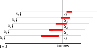
a)	b)
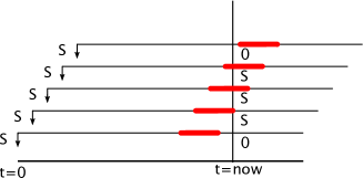
c)

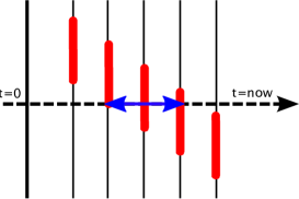
Figure 1: Graphical representation of population synthesis modelling. Time runs left to right from the Big Bang ($t=0$) until now in finite time steps, $\Delta t$. Stars formed at $0$ to $4\Delta t$ are shown, with corresponding star formation rates $S_{0},$ $S_{1}$, …, but in a realistic simulation there may be many thousands of time steps. Stars evolve from left to right along horizontal lines which, when they are in the phase of interest that is to be counted, they are thick and red (equivalent to $\delta_{j}=1$ in Eq. (3), $\delta_{j}=0$ otherwise). Stars are counted when the phase of interest intersects the vertical line which represents now. a) In an ideal population model, at each time step the star formation rate varies ($S_{0}\neq S_{1}\neq S_{2}\dots$) and the properties of the stars also vary (indicated by the change in colour and length of time spent in the phase of interest). b) In a simplified model, the stars all have the same properties (e.g. the same metallicity) and hence length of time in the phase of interest. The star formation rate is constant, i.e. $S=S_{0}=S_{1}=S_{2}\dots$. c) Instead of performing an expensive convolution over many models, the problem is rotated by $90^{\circ}$ and population statistics are calculated from a single model run represented by the horizontal dashed black line. The region denoted by the blue arrow is the phase of interest and the evolutionary model set has to be calculated only once, so the calculation is relatively cheap.

The vector $\mathbf{Z}$ represents model input parameters, such as metallicity, and input distributions which can change with the time of birth of the stars. The vector $\mathbf{X}$ denotes the many parameters which affect stellar evolution, such as metallicity, rotation rate, mass-loss prescription and mixing-length parameter. The function $\delta_{j}$ factors in stellar evolution, so is a function of $\mathbf{X}$, $\mathbf{Z}$ and $\tau$. The probability, $\psi_{i}$, is a function of at least mass, perhaps also metallicity (hence $\mathbf{Z}$) and, for binary stars, the companion mass and orbital properties also. If the function $\psi_{i}$ has $n$ parameters, the sum $\sum_{i}$ is implied over all of them. The large number of elements of this sum illustrates the parameter space problem we face even if $\mathbf{X}$ and $\mathbf{Z}$ are fixed.

In its most general form, Eq. (3) is a nasty convolution problem of the type faced by galactic chemical evolution models (Gibson et al.,, 2003). The problem can be simplified by fixing the stellar physics (i.e. $\mathbf{X}=\mathrm{constant}$ and $\mathbf{Z}=\mathrm{constant}$), the input distributions and assuming a constant star formation rate, e.g. $S=1$. The sum reduces to, as shown in Fig. 1,

$$N_{j} = \sum_{i}\psi_{i}\left(M,\dots\right)\sum_{\tau=0}^{t_{\mathrm{max}}}\delta_{j}\left(\tau\right)\,\delta\tau\,.$$ (2)

The parameter space wrapped into $\psi_{j}$ is still potentially very large, but the number of models to be calculated is greatly reduced because $\mathbf{X}$ and $\mathbf{Z}$ are fixed. We can also reduce the size of the sum over time by fixing the time step, $\delta\tau$, and allowing $\delta_{j}$ to take values between $0$ and $1$ corresponding to partial occupancy in phase $j$ during each time step. This is useful when calculating tables of model results with a fixed time resolution, e.g. for later use in a galactic chemical evolution context. The number of stars in a galaxy can be predicted by then scaling $S$ appropriately.

All the above is for just one type of star, denoted by $j$. In reality there are many different types of star and hence many different $N_{j}$. Our binary-star population synthesis code binary_c has more than 200 such types of star, both single and binary. It is also possible to count stars in bins, so that individual $N_{j}$ can be combined to create distributions. Differential measurements, such as number ratios, are more useful than simple predictions of the number of different types of stars in a population. One would hope that errors in approximations, such as our assumption that the star formation rate is constant, at least partly cancel out.

Further, the definition can be extended to count, say, stellar mass ejecta as we show in the Section 4. We set $\delta_{j}=\dot{M}_{j}\left(\tau\right)$, the rate of mass lost from a system as isotope $j$ as a function of stellar age, $\tau$. The normalised mass ejected as isotope $j$ from a population of single stars is defined as,

$$y_{j,\mathrm{sin}} = \frac{\sum_{i=M}\psi_{i}\sum_{\tau=0}^{t_{\mathrm{max}}}\dot{M}_{j}\left(\tau\right)\,\delta\tau}{\sum_{i=M}\psi_{i}M}\,,$$ (3)

and from a population of binary stars as,

$$y_{j,\mathrm{bin}} = \frac{\sum_{i=M_{1},M_{2},a}\psi_{i}\sum_{\tau=0}^{t_{\mathrm{max}}}\dot{M}_{j}\left(\tau\right)\,\delta\tau}{\sum_{i=M_{1},M_{2},a}\psi_{i}\left(M_{1}+M_{2}\right)}\,,$$ (4)

where $M$ is the initial mass of a single star and $M_{1}$, $M_{2}$ and $a$ are the initial primary mass, initial secondary mass and initial separation of a binary. The sums in the denominators are the total mass formed in stars in each population. This must be included to compare single to binary stars because binary systems have initially more mass, on average, than single stars. Note that $y_{j}$ are dimensionless.

4 Slow and Fast Parameters

Eq. (2) contains two main sets of parameters. The fast parameters are those that affect the input distributions, $\psi_{i}$. These include the slope and shape of the initial mass function, the secondary mass (or mass ratio) distribution and the initial orbital period distribution. These are called fast because changing $\psi_{i}$ does not require a recalculation of the stellar evolution model (which is embedded in $\delta_{j}$). Indeed, at any timestep in a stellar population calculation, as many different $\psi_{i}$ as desired can be calculated.

The slow parameters, on the other hand, require a complete recalculation of the stellar structure and evolution at every timestep. These are the $\mathbf{X}$ of Eq. (3). The calculation process is thus, in terms of computer speed, slow. Such parameters include the metallicity, mixing parameters, mass loss prescriptions and nuclear reaction rates. When stellar model grids are calculated, most of the slow parameters are fixed. Only one or a few parameters are then varied, such as the metallicity. Many of the constant parameters may not matter greatly to stellar evolution, but this often depends on the type of star under consideration, so the precise definition of our $j$ and hence $\delta_{j}$, and this dependence is often not known a priori.

In the following we demonstrate the dependence of a stellar population statistic, the amount of mass ejected from a stellar population as a particular isotope, on various model input parameters using Eqs. 3 and 4. The fast parameters affect the initial distributions, $\psi_{i}$, while the slow parameters affect the $\dot{M}_{j}\left(\tau\right)$, i.e. when and how much mass is ejected as isotope $j$ as a function of time. The initial parameters, $i$, are sampled on logarithmic grids, with single star masses in the range $0.1\leq M/\mathrm{M_{\odot}}\leq 80$ and $n_{M}=1000$ stars, binary component masses $M_{1}$ and $M_{2}$ are treated identically to $M$ but with $0.1\leq M_{2}\leq M_{1}$, $n_{M1}=100$ and $n_{M2}=100$, and separations in the range $3\leq a/\mathrm{R_{\odot}}\leq 10^{4}$, also with $n_{a}=100$ (so the total number of binary systems in each grid is $n_{M1}\times n_{M2}\times n_{a}=10^{6}$). At this resolution, errors in the relative mass ejected caused by a limited resolution and timestep are at most $2\%$.

1 Fast Parameters

In our example we have three distributions that define the fast parameters. These are the single or primary star initial mass distribution, the initial secondary mass distribution and the initial separation distribution. The single or primary star mass distribution is also known as the initial mass function. Our standard model is the Kroupa et al., (1993) initial mass function and we consider two alternatives from Chabrier, (2003) and Salpeter, (1955). Applying each gives us a range of uncertainty in stellar ejecta, $y_{j}$, as shown in Table 1.

We apply a similar process to the binary-star primary mass function which is assumed to be identical to that of single stars. The results are similar to those in single stars, but the impact of binary stars is seen in the reduced nitrogen and barium ejecta, because mass transfer truncates the evolution of thermally pulsing asymptotic giant branch stars, and in an increase in iron because of type Ia supernovae.

Our default distribution of secondary star masses is assumed to be flat in $q=M_{2}/M_{1}$, i.e. $\psi_{q}\propto q^{0}$, between $q=q_{\mathrm{min}}=0.1\,\mathrm{M}_{\odot}/M_{1}$ and $1$. We also consider distributions with $\psi_{q}\propto q^{0.5}$ (cf. Garmany et al.,, 1980) and $\psi_{q}\propto q^{-1.5}$, for illustration. In general, the changes to the mass ejecta, $y_{j}$, are smaller than changes caused by variation in the initial or primary star mass distribution.

Finally, we consider the distribution of binary orbits. This is set either by a distribution of orbital semi-major axes, $a$, or orbital periods, $P$, where both are related by Kepler’s law (we assume circular orbits). Our default distribution is $\psi_{a}\propto a^{-1}$, equivalent to Öpik, (1924). We also consider $\psi_{a}\propto a^{1}$ , $\psi_{a}\propto a^{-2}$ and combination of $\psi_{a}\propto a^{-0.7}$ and $10\leq a/\mathrm{R_{\odot}}\leq 1.3\times 10^{3}$ to match Goldberg et al., (2003). Table 1 shows that, as with the secondary-star mass distribution, reasonable changes in the separation distribution matter less than reasonable changes in the initial/primary star mass distribution.

Please note that the numbers calculated here are only a demonstration. A proper exploration of this problem would consider the more recent distributions of, e.g., Moe and Di Stefano, (2017) with their error bars. Such an exploration is unfortunately beyond the scope of this work.

Table 1: Masses of various isotopes ejected from a stellar population relative to the mass born into stars when reasonably varying fast parameters, i.e. the initial mass function in single stars, and in binary stars the primary star mass function, secondary star mass distribution and initial orbital separation within reasonable limits. These parameters are fast because they require only one run of the stellar evolution models.

Isotope	Single stars	Binary stars
	Vary $M$	Vary $M_{1}$	Vary $M_{2}$	Vary $a$
${}^{1}\mathrm{H}\times 10$	$1.9-3.7$	$1.9-3.6$	$1.7-2.2$	$1.6-2.6$
${}^{12}\mathrm{C}\times 10^{3}$	$4.6-15$	$5.7-18$	$3.8-6.1$	$4.0-6.2$
${}^{14}\mathrm{N}\times 10^{4}$	$9.6-24$	$8.1-19$	$7.6-9.8$	$7.9-9.5$
${}^{16}\mathrm{O}\times 10^{3}$	$8.4-30$	$9.6-32$	$7.2-10$	$7.1-11.5$
${}^{56}\mathrm{Fe}\times 10^{3}$	$1.0-3.0$	$2.5-5.4$	$1.3-2.7$	$0.9-3.4$
${}^{65}\mathrm{Cu}\times 10^{6}$	$10-32$	$8.8-28$	$7.0-9.2$	$8.0-12$
$\mathrm{Ba}\times 10^{9}$	$8.1-16$	$6.5-13$	$6.0-7.8$	$6.2-9.4$

2 Slow Parameters

There are many slow model parameters that alter the chemical ejecta from a population of stars. We limit our investigation to a population of 100% binary stars with fixed initial distributions of masses and orbital separations. Primary masses $M_{1}$ are distributed according to Kroupa et al., (1993) between $0.1$ and $80\mathrm{\,M_{\odot}}$, secondary mass ratios $q$ follow a flat distribution between $0.1\mathrm{\,M_{\odot}/M_{1}}$ and $1$, and separations, $a$, have a constant distribution in $\log a$ between $3$ and $10^{4}\mathrm{\,R}_{\odot}$.

The parameters we vary are metallicity in the range $10^{-4}\leq Z\leq 0.02$ (default is $0.02$), binary eccentricity $0\leq e\leq 1$ (default is $0$), red giant branch mass loss parameter $0.25\leq\eta\leq 0.75$ (default is $0.5$ using the Reimers,, 1975 formalism as defined in Hurley et al.,, 2000’s Eq. [106]), ${}^{13}\mathrm{C}$ pocket efficiency $0.01\leq\xi_{13}\leq 2.0$ (default is $1$, Izzard et al.,, 2006), wind loss rate during a Wolf-Rayet phase multiplier $0.1\leq f_{\mathrm{WR}}\leq 10$ (default is $1$, cf. Hurley et al.,, 2000’s section 7.1), an Eddington limit for accretion multiplied by $1$ or $10^{6}$ (default is $10^{6}$ i.e. no limit, Hurley et al.,, 2002’s Eq. [67]), a supernova kick velocity dispersion $0\leq\sigma_{\mathrm{SN}}/\mathrm{km}\,\mathrm{s}^{-1}\leq 400$ (default is $190\,\mathrm{km}\,\mathrm{s}^{-1}$, Hansen and Phinney,, 1997), companion reinforced attrition process (Tout and Eggleton,, 1988) parameter $0\leq B\leq 10^{4}$ (default is $0$, i.e. no reinforcement), common envelope parameter $\alpha_{\mathrm{CE}}=3$ (Hurley et al.,, 2002) and third dredge up parameters $-0.1\leq\Delta M_{\mathrm{c},\mathrm{min}}\leq 0$ (default $-0.07\mathrm{\,M_{\odot}}$) and $0\leq\lambda_{\mathrm{min}}\leq 1$ (default $0.8-37.5Z$ , Izzard et al.,, 2004a; Izzard and Tout,, 2004).

The normalised ejected mass of each isotope, $y_{j}$, is expanded as a Taylor series in the slow parameters labelled $k$ with values $x_{k}$,

$$y_{j}\left(x_{k}\right) = y_{j0}+\frac{dy_{j}}{dx_{k}}\left(x_{k}-x_{k0}\right)+\dots\approx y_{j0}+\left(1+T_{jk}\frac{\delta x_{k}}{\Delta x_{k}}\right)\,,$$ (5)

where $x_{k0}$ are the default values which one may consider best estimates, $y_{j0}$ are the ejecta corresponding to the default parameter set $x_{k0}$, $\delta x_{k}=x_{k}-x_{k0}$, and $x_{k}$ varies from $x_{k,\mathrm{min}}$ to $x_{k,\mathrm{min}}+\Delta x_{k}$. The matrix of derivatives,

$$T_{jk} = \frac{d\left(y_{j}/y_{j0}\right)}{d\left(x_{k}/\Delta x_{k}\right)}\,,$$ (6)

provides a relatively unbiased comparison of parameters because it measures the rate of change of dimensionless and normalised numbers, $y_{j}/y_{j0}$ and $x_{k}/\Delta x_{k}$. A larger absolute value of $T_{jk}$ thus reflects greater sensitivity of amount of isotope $j$ ejected to the parameter $k$. One drawback of this approach is that it only considers the linear terms in the Taylor expansion: it is possible that, at second or higher order, the effects of changing two parameters cancel each other out. Such considerations are beyond the scope of this work.

Table 2 shows how the $T_{jk}$ vary with each model parameter. Absolute values above $0.1$ are marked in bold/red. These are the parameters to which the chemical ejecta are most sensitive. As an example, the ejecta of most isotopes vary little with the ${}^{13}\mathrm{C}$ $s$-process pocket efficiency. The exception is barium, an $s$-process element, which is very sensitive to the efficiency of $s$-processing, as one would expect. While this is a trivial example, it is perhaps less obvious that the ejection of ${}^{16}\mathrm{O}$ depends ten times more weakly on the common envelope parameter, $\alpha_{\mathrm{CE}}$, than does ${}^{14}\mathrm{N}$.

Table 2: Ejecta dependence on various model parameters as measured by $T_{jk}$, the magnitude of which is an attempt to measure the dependence on each model parameter $k$ of the relative mass ejected from a population of stars as isotope $j$ (Eq. 6, symbols are defined in the main text). $x^{(y)}$ means $x\times 10^{y}$. The numbers highlighted in red/bold have an absolute value exceeding $0.1$ and are the most sensitive to their parameter.

Isotope	Model Parameter
	$Z$	$\xi_{\mathrm{C}13}$	$f_{\mathrm{WR}}$	$\alpha_{\mathrm{CE}}$	$\Delta M_{\mathrm{c},\mathrm{min}}$	$e$	$f_{\mathrm{Edd}}$	$\eta_{\mathrm{GB}}$	$\lambda_{\mathrm{min}}$	$\sigma_{\mathrm{SN}}$
${}^{1}\mathrm{H}$	$\mathbf{-1.9^{(-1)}}$	$1.2^{(-4)}$	$-3.6^{(-3)}$	$-1.6^{(-2)}$	$5.2^{(-3)}$	$4.5^{(-2)}$	$-3.5^{(-4)}$	$8.2^{(-3)}$	$-9.9^{(-3)}$	$-5.3^{(-3)}$
${}^{12}\mathrm{C}$	$6.0^{(-2)}$	$-1.8^{(-3)}$	$\mathbf{1.0^{(-1)}}$	$\mathbf{1.1^{(-1)}}$	$-7.1^{(-2)}$	$\mathbf{-1.6^{(-1)}}$	$-1.8^{(-2)}$	$-5.0^{(-2)}$	$\mathbf{1.6^{(-1)}}$	$4.6^{(-2)}$
${}^{14}\mathrm{N}$	$\mathbf{-6.5^{(-1)}}$	$-1.3^{(-4)}$	$-5.9^{(-3)}$	$\mathbf{-4.1^{(-1)}}$	$-3.8^{(-3)}$	$9.4^{(-2)}$	$-2.7^{(-5)}$	$-1.9^{(-2)}$	$1.8^{(-2)}$	$2.7^{(-2)}$
${}^{16}\mathrm{O}$	$8.8^{(-2)}$	$-2.6^{(-3)}$	$\mathbf{-4.9^{(-1)}}$	$-2.3^{(-2)}$	$2.0^{(-3)}$	$-5.3^{(-2)}$	$1.2^{(-3)}$	$-1.0^{(-2)}$	$-4.0^{(-4)}$	$1.0^{(-1)}$
${}^{56}\mathrm{Fe}$	$\mathbf{9.6^{(-1)}}$	$-3.9^{(-4)}$	$\mathbf{-1.8^{(-1)}}$	$\mathbf{2.3^{(-1)}}$	$1.8^{(-3)}$	$\mathbf{-2.5^{(-1)}}$	$5.8^{(-2)}$	$-9.3^{(-3)}$	$-2.5^{(-3)}$	$2.5^{(-2)}$
${}^{65}\mathrm{Cu}$	$\mathbf{-7.2^{(-1)}}$	$-5.8^{(-4)}$	$-7.5^{(-2)}$	$\mathbf{-3.1^{(-1)}}$	$1.0^{(-3)}$	$7.8^{(-2)}$	$1.1^{(-3)}$	$-2.0^{(-2)}$	$1.4^{(-3)}$	$7.0^{(-2)}$
$\mathrm{Ba}$	$\mathbf{-2.2}$	$\bm{1.3}$	$2.5^{(-2)}$	$\mathbf{-2.6^{(-1)}}$	$-9.1^{(-2)}$	$\mathbf{1.1^{(-1)}}$	$-2.2^{(-3)}$	$-7.1^{(-2)}$	$\mathbf{2.0^{(-1)}}$	$3.1^{(-3)}$

5 Matching Models to Observations, and Models to Models

The general problem of matching model results, with their distributions of input parameters, to many observations is one that is, in every sense of the word, non-trivial. The size of the parameter space is daunting. Efforts like those mentioned in Sec. 2 reduce the number of parameters to only those that matter for a given observational data set of a particular type of star. Perhaps the greatest problem is in how to match all stars from as many data sets as possible simultaneously, thus provide the best possible constraints. The solution to this problem is beyond our current reach.

Frameworks to match a grid of models to an individual observed star are relatively well developed. A good example is the Bayesian algorithm BONNSAI (Schneider et al.,, 2014b, 2017). Given, say, the effective temperature, luminosity and surface abundances of the star, all the models in a particular grid are compared to it to determine – in an automated way – which fits best. Bayesian techniques also naturally give posterior distributions of parameters, hence associated error bars. BONNSAI also tests that model resolution is sufficient to believe the best fit. Other, related techniques such as Markov-chain Monte Carlo (MCMC) methods are starting to be employed by the community, particularly in the hunt for the progenitors of gravitational wave sources (e.g. Mandel and O’Shaughnessy,, 2010). The next big step will be to use such techniques in general, e.g. to match the data of Gaia, to whole population models.

When matching a large number of stars to population models, the selection effects of the survey in question should also be taken into account. All surveys, even those that are ’complete’, have some kind of selection bias. In many cases, a simple cut in say magnitude or surface gravity, which effectively selects stars in a particular phase of evolution, is sufficient and easy to fit into a Bayesian analysis (e.g. Casagrande et al.,, 2014; Izzard et al.,, 2017). Modern surveys often have a well described ’selection function’ which describes in a probabilistic way the various biases inherent to their sample, e.g. the Gaia-ESO survey (Stonkutė et al.,, 2016). However, older data often has poorly defined selection effects and, in some cases, data is selected ’by eye’ which renders its modelling essentially impossible.

Finally, our computation models must be tested and verified. One way to do this is to compare the models of one group against those of another to test for consistency. In the case that both groups use identical input physics, the results should be the same. The POPCORN collaboration tried to do this, pitting binary_c against the SeBa, Startrack and Brussels population synthesis codes (Toonen et al.,, 2014, and references therein). The four codes were, for the most part, consistent, which at least suggests we are getting the numerics right. Whether the physics they employed is true to life is another question which POPCORN did not try to answer.

6 Headline News in Population Synthesis

There are many fields in which population synthesis has shown itself to be useful. The colours of galaxies are now accepted to be influenced by binary stars, for example the UV emission of elliptical galaxies is influenced by subdwarf-O/B stars which can only form in binaries (Han et al.,, 2007). Massive blue straggler stars form when binaries transfer mass or merge and are common enough to be measurable in the present day mass function of young stellar clusters (Schneider et al.,, 2014a). Similarly, type II supernovae can be delayed in binary systems, and predictions have recently been made that analyse the multi-dimensional parameter space of such objects in great detail (Zapartas et al.,, 2017). The rates of more exotic channels, such as long and short gamma-ray bursts, can also only be predicted by population synthesis (Izzard et al.,, 2004b; Szécsi,, 2017). Binary stars affect stellar evolution such that the chemical yields of elements are altered, e.g. through type Ia supernova and nova channels. Population synthesis is required to estimate rates and yields of such events (e.g. Claeys et al.,, 2014) and the effect of mass transfer on chemistry more generally (De Donder and Vanbeveren,, 2002b; Izzard et al.,, 2017). Mass transfer also makes chemically peculiar stars. The number and properties of these – such as orbital periods and eccentricities – can be used to better understand stellar interior mixing, mass transfer, tides and interactions with circumstellar and circumbinary discs (Jorissen et al.,, 2009; Izzard et al.,, 2010; Dermine et al.,, 2013 and Fig. 2).

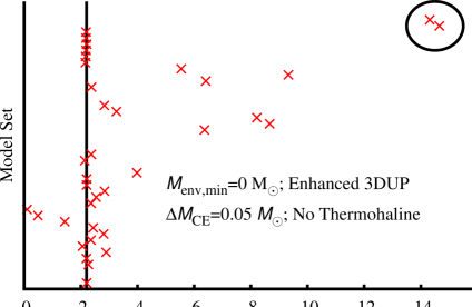
Figure 2: The ratio of carbon-enhanced extremely metal-poor (CEMP) stars to all extremely metal-poor stars (EMP) in the Galactic halo as predicted by our population nucleosynthesis code, binary_c, as a function different input physics, here labelled ’model sets’. Full details of the model sets and general problem are in Izzard et al., (2009). Briefly, CEMP stars are red giants that formed by accretion from a carbon-star companion in the past (Abate et al.,, 2015 shows our latest models). Each model set predicts a CEMP/EMP ratio which should to be compared to the observed ratio in the Galactic halo which is 20%. Most of our model sets predict a $2\%$ CEMP/EMP ratio which is wrong by an order of magnitude. Only two model sets approach the observed 20%. These both require all the following. 1) Third dredge up must be efficient in low-mass stars, right down to $0.9\mathrm{\,M_{\odot}}$, at low metallicity (here $Z=10^{-4}$). 2) Third dredge up must be efficient in stars with small envelope masses (the minimum envelope mass for third dredge up, $M_{\mathrm{env,}\mathrm{min}},$ is zero here). 3) A small amount of accretion occurs during any common-envelope phase ($\Delta M_{\mathrm{CE}}=0.05\mathrm{\,M_{\odot}}$). 4) Thermohaline mixing in accreting stars is suppressed. At the time of writing the original paper (2009) it was considered impossible for $0.9\mathrm{\,M_{\odot}}$ stars to undergo third dredge up and hence become carbon stars. More recent works have shown that not only is this possible it is quite likely (e.g. Karakas,, 2010b). The population synthesis modelling results encouraged detailed stellar evolutionists to examine stars of both low mass and low metallicity in far more detail, resulting in a far better understanding of the problem (e.g. Fishlock et al.,, 2014; Matrozis and Stancliffe,, 2016, 2017).

We have also recently improved our binary_c models to combine them with a model of the Galaxy and Magellanic Clouds to predict the number of hypervelocity stars that originate from the Large Magellanic Cloud (Boubert et al.,, 2017b). These young stars are moving so fast that they are not bound to our Galaxy. One way they can be made is in binary systems in which one star explodes as a supernova leaving the companion to escape. We predicted large numbers of such stars, their positions on the sky and their stellar properties. Our predictions will soon be tested by Gaia.

The recent advances in gravitational wave physics have certainly put population synthesis in the headlines. Merging stellar-mass black holes and neutron stars are all the rage, and the predictions of population synthesis models of such objects can be put to the test (e.g. Belczynski et al.,, 2016, and many other works). The systematic uncertainties on such rate estimates are large, often many orders of magnitude. These realistically reflect our ignorance of the physical processes involved, especially binary problems such as common envelope evolution, and their sensitivity to the many model parameters which are often known only approximately.

7 Not Any Colour You Like…

A persistent claim we have heard over the years is that, with population synthesis, you can get whatever you like out of the models. Indeed, with so many parameters to play with this may seem at first glance to be true. An important counterargument, however, is that number statistics can be predicted by population synthesis with quantified uncertainties. It is these uncertainties that are large and perhaps this is where the ’whatever you like’ myth originates. In such cases it is important to identify the parameters in the model which lead to the large uncertainties and pin these down, either by observation, experiment or development of a better theory. By some this is called progress and, with more and better data, it is simply no longer possible to get any result one would like. Also, ignorance of the effect of uncertain parameters, be they initial distributions of stars or the choice of input physics, does not mean the error on such model predictions is zero. Population synthesis at least allows us to quantify some of these systematic errors and remains a very powerful tool to investigate the evolution of both single and binary stars in the 21st century.

References

- Abate et al., (2013) Abate, C., Pols, O. R., Izzard, R. G., Mohamed, S. S., and de Mink, S. E. 2013. Wind Roche-lobe overflow: Application to carbon-enhanced metal-poor stars. A&A, 552(Apr.), A26.
- Abate et al., (2015) Abate, C., Pols, O. R., Stancliffe, R. J., Izzard, R. G., Karakas, A. I., Beers, T. C., and Lee, Y. S. 2015. Modelling the observed properties of carbon-enhanced metal-poor stars using binary population synthesis. A&A, 581(Sept.), A62.
- Belczynski et al., (2016) Belczynski, K., Holz, D. E., Bulik, T., and O’Shaughnessy, R. 2016. The first gravitational-wave source from the isolated evolution of two stars in the 40-100 solar mass range. Nature, 534(June), 512–515.
- Boubert et al., (2017a) Boubert, D., Fraser, M., Evans, N. W., Green, D. A., and Izzard, R. G. 2017a. Binary companions of nearby supernova remnants found with Gaia. A&A, 606(Sept.), A14.
- Boubert et al., (2017b) Boubert, D., Erkal, D., Evans, N. W., and Izzard, R. G. 2017b. Hypervelocity runaways from the Large Magellanic Cloud. MNRAS, 469(Aug.), 2151–2162.
- Brott et al., (2011) Brott, I., Evans, C. J., Hunter, I., de Koter, A., Langer, N., Dufton, P. L., Cantiello, M., Trundle, C., Lennon, D. J., de Mink, S. E., Yoon, S.-C., and Anders, P. 2011. Rotating massive main-sequence stars. II. Simulating a population of LMC early B-type stars as a test of rotational mixing. A&A, 530(June), A116.
- Casagrande et al., (2014) Casagrande, L., Silva Aguirre, V., Stello, D., Huber, D., Serenelli, A. M., Cassisi, S., Dotter, A., Milone, A. P., Hodgkin, S., Marino, A. F., Lund, M. N., Pietrinferni, A., Asplund, M., Feltzing, S., Flynn, C., Grundahl, F., Nissen, P. E., Schönrich, R., Schlesinger, K. J., and Wang, W. 2014. Strömgren Survey for Asteroseismology and Galactic Archaeology: Let the SAGA Begin. ApJ, 787(June), 110.
- Chabrier, (2003) Chabrier, G. 2003. Galactic Stellar and Substellar Initial Mass Function. PASP, 115(July), 763–795.
- Chieffi and Limongi, (2004) Chieffi, A., and Limongi, M. 2004. Explosive Yields of Massive Stars from Z=0 to Z = Z⊙. ApJ, 608(June), 405–410.
- Claeys et al., (2014) Claeys, J. S. W., Pols, O. R., Izzard, R. G., Vink, J., and Verbunt, F. W. M. 2014. Theoretical uncertainties of the Type Ia supernova rate. A&A, 563(Mar.), A83.
- De Donder and Vanbeveren, (2002a) De Donder, E., and Vanbeveren, D. 2002a. The chemical evolution of the solar neighbourhood: the effect of binaries. New Astronomy, 7(Mar.), 55–84.
- De Donder and Vanbeveren, (2002b) De Donder, E., and Vanbeveren, D. 2002b. The chemical evolution of the solar neighbourhood: the effect of binaries. New Astronomy, 7(Mar.), 55–84.
- De Marco and Izzard, (2017) De Marco, O., and Izzard, R. G. 2017. Dawes Review 6: The Impact of Companions on Stellar Evolution. PASA, 34(Jan.), e001.
- de Mink et al., (2013) de Mink, S. E., Langer, N., Izzard, R. G., Sana, H., and de Koter, A. 2013. The Rotation Rates of Massive Stars: The Role of Binary Interaction through Tides, Mass Transfer, and Mergers. ApJ, 764(Feb.), 166.
- Dermine et al., (2013) Dermine, T., Izzard, R. G., Jorissen, A., and Van Winckel, H. 2013. Eccentricity-pumping in post-AGB stars with circumbinary discs. A&A, 551(Mar.), A50.
- Duchêne and Kraus, (2013) Duchêne, G., and Kraus, A. 2013. Stellar Multiplicity. ARA&A, 51(Aug.), 269–310.
- Eggleton et al., (1989) Eggleton, P. P., Fitchett, M. J., and Tout, C. A. 1989. The distribution of visual binaries with two bright components. ApJ, 347(Dec.), 998–1011.
- Eldridge et al., (2017) Eldridge, J. J., Stanway, E. R., Xiao, L., McClelland, L. A. S., Taylor, G., Ng, M., Greis, S. M. L., Bray, J. C., and . 2017. Binary Population and Spectral Synthesis Version 2.1: construction, observational verification and new results. ArXiv e-prints, Oct.
- Fishlock et al., (2014) Fishlock, C. K., Karakas, A. I., and Stancliffe, R. J. 2014. The effect of including molecular opacities of variable composition on the evolution of intermediate-mass AGB stars. MNRAS, 438(Feb.), 1741–1750.
- Fuhrmann et al., (2017) Fuhrmann, K., Chini, R., Kaderhandt, L., and Chen, Z. 2017. Multiplicity among Solar-type Stars. ApJ, 836(Feb.), 139.
- Garmany et al., (1980) Garmany, C. D., Conti, P. S., and Massey, P. 1980. Spectroscopic studies of O type stars. IX - Binary frequency. ApJ, 242(Dec.), 1063–1076.
- Gibson et al., (2003) Gibson, B. K., Fenner, Y., Renda, A., Kawata, D., and Lee, H.-c. 2003. Galactic Chemical Evolution. PASA, 20, 401–415.
- Goldberg et al., (2003) Goldberg, D., Mazeh, T., and Latham, D. W. 2003. On the Mass-Ratio Distribution of Spectroscopic Binaries. ApJ, 591(July), 397–405.
- Han et al., (2007) Han, Z., Podsiadlowski, P., and Lynas-Gray, A. E. 2007. A binary model for the UV-upturn of elliptical galaxies. MNRAS, 380(Sept.), 1098–1118.
- Hansen and Phinney, (1997) Hansen, B. M. S., and Phinney, E. S. 1997. The pulsar kick velocity distribution. MNRAS, 291(Nov.), 569+.
- Hurley et al., (2000) Hurley, J. R., Pols, O. R., and Tout, C. A. 2000. Comprehensive analytic formulae for stellar evolution as a function of mass and metallicity. MNRAS, 315(July), 543–569.
- Hurley et al., (2002) Hurley, J. R., Tout, C. A., and Pols, O. R. 2002. Evolution of binary stars and the effect of tides on binary populations. MNRAS, 329(Feb.), 897–928.
- Hut, (1981) Hut, P. 1981. Tidal evolution in close binary systems. Astronomy and Astrophysics, 99(June), 126–140.
- Izzard and Tout, (2004) Izzard, R. G., and Tout, C. A. 2004. A binary origin for low-luminosity carbon stars. MNRAS, 350(May), L1–4.
- Izzard et al., (2004a) Izzard, R. G., Tout, C. A., Karakas, A. I., and Pols, O. R. 2004a. A new synthetic model for asymptotic giant branch stars. MNRAS, 350(May), 407–426.
- Izzard et al., (2004b) Izzard, R. G., Ramirez-Ruiz, E., and Tout, C. A. 2004b. Formation rates of core-collapse supernovae and gamma-ray bursts. MNRAS, 348(Mar.), 1215–1228.
- Izzard et al., (2006) Izzard, R. G., Dray, L. M., Karakas, A. I., Lugaro, M., and Tout, C. A. 2006. Population nucleosynthesis in single and binary stars. I. Model. A&A, 460(Dec.), 565–572.
- Izzard et al., (2009) Izzard, R. G., Glebbeek, E., Stancliffe, R. J., and Pols, O. R. 2009. Population synthesis of binary carbon-enhanced metal-poor stars. A&A, 508(Dec.), 1359–1374.
- Izzard et al., (2010) Izzard, R. G., Dermine, T., and Church, R. P. 2010. White-dwarf kicks and implications for barium stars. A&A, 523(Nov.), A10.
- Izzard et al., (2017) Izzard, R. G., Preece, H., Jofre, P., Halabi, G. M., Masseron, T., and Tout, C. A. 2017. Binary stars in the Galactic thick disc. ArXiv e-prints, Sept.
- Jorissen et al., (2009) Jorissen, A., Frankowski, A., Famaey, B., and van Eck, S. 2009. Spectroscopic binaries among Hipparcos M giants. III. The eccentricity - period diagram and mass-transfer signatures. A&A, 498(May), 489–500.
- José and Hernanz, (1998) José , J., and Hernanz, M. 1998. Nucleosynthesis in Classical Novae: CO versus ONe White Dwarfs. ApJ, 494(Feb.), 680.
- Karakas, (2010a) Karakas, A. I. 2010a. Updated stellar yields from asymptotic giant branch models. MNRAS, 403(Apr.), 1413–1425.
- Karakas, (2010b) Karakas, A. I. 2010b. Updated stellar yields from asymptotic giant branch models. MNRAS, 403(Apr.), 1413–1425.
- Karakas et al., (2002) Karakas, A. I., Lattanzio, J. C., and Pols, O. R. 2002. Parameterising the third dredge-up in asymptotic giant branch stars. PASA, 19, 515–526.
- Kroupa, (2001) Kroupa, P. 2001. On the variation of the initial mass function. MNRAS, 322(Apr.), 231–246.
- Kroupa et al., (1993) Kroupa, P., Tout, C.A., and Gilmore, G. 1993. The distribution of low-mass stars in the Galactic disc. MNRAS, 262(June), 545–587.
- Kruckow and et al., (2017) Kruckow, M., and et al. 2017. Hunting for gravitational wave sources: Binary evolution with the stellar-grid based code STARBURST. A&Ain prep.
- Mandel and O’Shaughnessy, (2010) Mandel, I., and O’Shaughnessy, R. 2010. Compact binary coalescences in the band of ground-based gravitational-wave detectors. Classical and Quantum Gravity, 27(11), 114007.
- Matrozis and Stancliffe, (2016) Matrozis, E., and Stancliffe, R. J. 2016. Radiative levitation in carbon-enhanced metal-poor stars with s-process enrichment. A&A, 592(July), A29.
- Matrozis and Stancliffe, (2017) Matrozis, E., and Stancliffe, R. J. 2017. Rotational mixing in carbon-enhanced metal-poor stars with s-process enrichment. A&A (in press), arXiv 1707.09434, July.
- Moe and Di Stefano, (2017) Moe, M., and Di Stefano, R. 2017. Mind Your Ps and Qs: The Interrelation between Period (P) and Mass-ratio (Q) Distributions of Binary Stars. ApJS, 230(June), 15.
- Öpik, (1924) Öpik, E. 1924. Statistical Studies of Double Stars: On the Distribution of Relative Luminosities and Distances of Double Stars in the Harvard Revised Photometry North of Declination -31. Publications of the Tartu Astrofizica Observatory, 25.
- Paxton et al., (2011) Paxton, B., Bildsten, L., Dotter, A., Herwig, F., Lesaffre, P., and Timmes, F. 2011. Modules for Experiments in Stellar Astrophysics (MESA). ApJS, 192(Jan.), 3.
- Paxton et al., (2015) Paxton, B., Marchant, P., Schwab, J., Bauer, E. B., Bildsten, L., Cantiello, M., Dessart, L., Farmer, R., Hu, H., Langer, N., Townsend, R. H. D., Townsley, D. M., and Timmes, F. X. 2015. Modules for Experiments in Stellar Astrophysics (MESA): Binaries, Pulsations, and Explosions. ApJS, 220(Sept.), 15.
- Raghavan et al., (2010) Raghavan, D., McAlister, H. A., Henry, T. J., Latham, D. W., Marcy, G. W., Mason, B. D., Gies, D. R., White, R. J., and ten Brummelaar, T. A. 2010. A Survey of Stellar Families: Multiplicity of Solar-type Stars. ApJS, 190(Sept.), 1–42.
- Reimers, (1975) Reimers, D. 1975. Circumstellar envelopes and mass loss of red giant stars. Springer-Verlag New York, Inc., 1975. Pages 229–256.
- Salpeter, (1955) Salpeter, E. E. 1955. The Luminosity Function and Stellar Evolution. ApJ, 121(Jan.), 161.
- Sana et al., (2012) Sana, H., de Mink, S. E., de Koter, A., Langer, N., Evans, C. J., Gieles, M., Gosset, E., Izzard, R. G., Le Bouquin, J.-B., and Schneider, F. R. N. 2012. Binary Interaction Dominates the Evolution of Massive Stars. Science, 337(July), 444.
- Schneider et al., (2014a) Schneider, F. R. N., Izzard, R. G., de Mink, S. E., Langer, N., Stolte, A., de Koter, A., Gvaramadze, V. V., Hußmann, B., Liermann, A., and Sana, H. 2014a. Ages of Young Star Clusters, Massive Blue Stragglers, and the Upper Mass Limit of Stars: Analyzing Age-dependent Stellar Mass Functions. ApJ, 780(Jan.), 117.
- Schneider et al., (2014b) Schneider, F. R. N., Langer, N., de Koter, A., Brott, I., Izzard, R. G., and Lau, H. H. B. 2014b. Bonnsai: a Bayesian tool for comparing stars with stellar evolution models. A&A, 570(Oct.), A66.
- Schneider et al., (2017) Schneider, F. R. N., Castro, N., Fossati, L., Langer, N., and de Koter, A. 2017. BONNSAI: correlated stellar observables in Bayesian methods. A&A, 598(Feb.), A60.
- Siess et al., (2013) Siess, L., Izzard, R. G., Davis, P. J., and Deschamps, R. 2013. BINSTAR: a new binary stellar evolution code. Tidal interactions. A&A, 550(Feb.), A100.
- Stancliffe et al., (2007) Stancliffe, R. J., Glebbeek, E., Izzard, R. G., and Pols, O. R. 2007. Carbon-enhanced metal-poor stars and thermohaline mixing. A&A, 464(Mar.), L57–L60.
- Stonkutė et al., (2016) Stonkutė, E., Koposov, S. E., Howes, L. M., Feltzing, S., Worley, C. C., Gilmore, G., Ruchti, G. R., Kordopatis, G., Randich, S., Zwitter, T., Bensby, T., Bragaglia, A., Smiljanic, R., Costado, M. T., Tautvaišienė, G., Casey, A. R., Korn, A. J., Lanzafame, A. C., Pancino, E., Franciosini, E., Hourihane, A., Jofré, P., Lardo, C., Lewis, J., Magrini, L., Monaco, L., Morbidelli, L., Sacco, G. G., and Sbordone, L. 2016. The Gaia-ESO Survey: the selection function of the Milky Way field stars. MNRAS, 460(July), 1131–1146.
- Szécsi, (2017) Szécsi, D. 2017. Single and binary stellar progenitors of long-duration gamma-ray bursts. ArXiv e-prints, Oct.
- Toonen et al., (2014) Toonen, S., Claeys, J. S. W., Mennekens, N., and Ruiter, A. J. 2014. PopCORN: Hunting down the differences between binary population synthesis codes. A&A, 562(Feb.), A14.
- Toonen et al., (2016) Toonen, S., Hamers, A., and Portegies Zwart, S. 2016. The evolution of hierarchical triple star-systems. Computational Astrophysics and Cosmology, 3(Dec.), 6.
- Tout and Eggleton, (1988) Tout, C. A., and Eggleton, P. P. 1988. Tidal enhancement by a binary companion of stellar winds from cool giants. MNRAS, 231(Apr.), 823–831.
- Tout et al., (1997) Tout, C. A., Aarseth, S. J., Pols, O. R., and Eggleton, P. P. 1997. Rapid binary star evolution for N-body simulations and population synthesis. MNRAS, 291(Nov.), 732.
- Woosley and Weaver, (1995) Woosley, S. E., and Weaver, T. A. 1995. The Evolution and Explosion of Massive Stars. II. Explosive Hydrodynamics and Nucleosynthesis. ApJS, 101(Nov.), 181.
- Zapartas et al., (2017) Zapartas, E., de Mink, S. E., Izzard, R. G., Yoon, S.-C., Badenes, C., Götberg, Y., de Koter, A., Neijssel, C. J., Renzo, M., Schootemeijer, A., and Shrotriya, T. S. 2017. Delay-time distribution of core-collapse supernovae with late events resulting from binary interaction. A&A, 601(May), A29.
Index
- Bayesian methods §5
- big data id4.id1
- binary orbit §1
- binary stars §1
- binary_c §2
- chemical yields §3
- dendrology §2
- fast parameters §1
- gratuitous pink floyd reference §7
- initial binary distributions §1
- mass ejecta §3
- Matching observations to models §5
- population synthesis id4.id1
- slow parameters §2
- stellar accountancy §3
- stellar number counting §3
- stellar parameter space §1
- synthetic stellar models §2