Parameter Synthesis Problems for
Parametric Timed Automata

Abstract

We consider the parameter synthesis problem of parametric timed automata (PTAs). The problem is, given a PTA and a property, to compute the set of valuations of the parameters under which the resulting timed automaton satisfies the property. Such a set of parameter valuations is called a feasible region for the PTA and the property. The problem is known undecidable in general. This paper, however, presents our study on some decidable sub-classes of PTAs and proposes efficient parameter synthesis algorithms for them. Our contribution is four-fold: i) the study of the PTAs (called one-one PTAs) with one parameter and one parametrically constrained clock and an algorithm for computing the feasible region for a one-one PTA and a property; ii) the study of the PTAs with lower-bound or with upper-bound parameters only and a procedure to construct the feasible region for such a PTA with one parametrically constrained clock and a property; iii) a theorem showing that the feasible region for a PTA with both the lower-bound and upper-bound parameters (i.e. a general L/U PTA) and a property which has existential quantifiers only is a “single connected” set; and iv) a support vector machine based algorithm to identify the boundary of the feasible region for a general L/U PTA and a property. We belief that these results contribute to advancing the theoretical investigations of the parameter synthesis problem for PTAs, and support to exploit machine learning methods to give potentially more practical synthesis algorithms as well.

I Introduction

Real-time applications are increasing importance, so are their complexity and requirements for trustworthiness, in the era of Internet of Things (IoT), especially in the areas of industrial control and smart homes. Consider, for example, the control system of a boiler used in house. Such a system is required to switch on the gas within a certain bounded period of time when the water gets too cold. Indeed, the design and implementation of the system not only have to guarantee the correctness of system functionalities, but also need to assure that the application is in compliance with the non-functional requirements, that are timing constraints in this case.

Timed automata (TAs) [1, 2] are widely used for modeling and verification of real-time systems. However, one disadvantage of the TA-based approach is that it can only be used to verify concrete properties, i.e., properties with concrete values of all timing parameters occurring in the system. Typical examples of such parameters are upper and lower bounds of computation time, message delay and time-out. This makes the traditional TA-based approach not ideal for the design of real-time applications because in the design phase concrete values are often not available. This problem is usually dealt with extensive trial-and-error and prototyping activities to find out what concrete values of the parameters are suitable. This approach of design is costly, laborious, and error-prone, for at least two reasons: (1) many trials with different parameter configurations suffer from unaffordable costs, without enough assurance of a safety standard because a sufficient coverage of configurations is difficult to achieve; (2) little or no feedback information is provided to the developers to help improve the design when a system malfunction is detected.

I-A Decidable parametric timed automata

To mitigate the limitations of the TA-based approach, parametric timed automata (PTAs) are proposed [3, 4, 5, 6], which allow more general constraints on invariants of nodes (or states) and guards of edges (or transitions) of an automaton. Informally, a clock $x$ of a PTA $\mathcal{A}$ is called a parametrically constrained clock if $x$ and some parameters both occur in a constraint of $\mathcal{A}$. Obviously, given any valuation of the parameters in a PTA, we obtain a concrete TA. One of the most important questions of PTAs is the synthesis problem, that is, for a given property to compute the entire set of valuations of the parameters for a PTA such that when the parameters are instantiated by these valuations, the resulting TAs all satisfy the property. The synthesis problem for general PTAs is known to be undecidable. There are, however, several proposals to restrict the general PTAs from different perspectives to gain decidability. Two kinds of restrictions that are being widely investigated are (1) on the number of clocks/parameters in the PTA; and (2) on the way in which parameters are bounded, such as the L/U PTAs [6].

I-B Our contribution

The first part of our work is about restrictions of the first kind above, and it considers the PTAs, which we later refer to as one-one PTAs, which have one parametrically constrained clock and one parameter, but allowing arbitrary number of other clocks. We extend the result of [3] and provide an algorithm to construct the feasible parameter region explicitly for a one-one PTA and a property.

The second part of our work studies L/U automata. In an L/U automaton, each parameter occurs either as a lower-bound only in the invariants and guards, or as an upper-bound only therein. In other words, a parameter in an L/U automaton cannot occur as both a lower-bound and an upper-bound of clocks. We call an L/U automaton an L-automaton (resp. U-automaton) if all parameters occur only as lower-bounds (resp. upper-bounds). The results of [6] show that the emptiness problem for L/U automata is decidable. They also extend the model checker UPPAAL to synthesize linear parameter constraints for L/U-automata. Decidability results for L/U automata have been further investigated [7]. There for L-automata and U-automata, the authors solve the synthesis problem for a restricted class of liveness properties, i.e. the existence of an infinite accepting run for the automaton. Our work in this paper, instead of the liveness property considered in [7], considers an other class of properties. These properties are generally generally described as formulas in temporal logic of the form $\exists\Diamond\phi$ and $\forall\Box\phi$, and their satisfiction by a PTA can be treated as reachability properties. Here, $\phi$ is a state property, $\exists$ (or $\forall$) means there exists (resp. for all) runs. For these properties, we solve the parameter synthesis problem for L-automata and U-automata by explicitly constructing the feasible parameter regions.

Furthermore, for general model of L/U automata, we show that the feasible parameter region forms a “single connected” set provided that the property contains existential quantifiers only. Being connected here means that for any pair of valuations $v$ and $v^{\prime}$ there is at least one sequence of $v=v_{1},\ldots,v_{\ell}=v^{\prime}$ feasible valuations, such that the Euclidean distance between $v_{i}$ and $v_{i+1}$ is $1$. This topological property of feasible regions allows us to develop a machine learning algorithm based on support vector machine (SVM) to identify the boundary of a feasible region.

I-C Related work

The earliest work on PTAs goes back to 90’s [3] by Alur, et al, where the general undecidability of the reachability emptiness for a PTA with three or more parametrically constrained clocks is proved. There, a backward computation based algorithm to solve the emptiness problem is also presented for a nontrivial class of PTAs which have only one parametrically constrained clock. It is also shown there that for the remaining class of PTAs, that is the class of PTAs with exactly two parametrically constrained clocks, the problem is closely related to various hard (viz. open) problems of logic and automata theory. A semi-algorithm based on expressive symbolic representation structures called parametric difference bound matrices is proposed in [4]. The algorithm uses accurate extrapolation techniques to speed up the reachability computation and ensure termination. The work in [8] proposes a class of PTAs in which a parameter cannot be shared by a lower bound constraint and an upper bound constraint. And, in this setting, the work there studies the Linear Temporal Logic (LTL) augmented with parameters.

A SMT-based method of computing under-approximation of the solution to this problem for L/U automata is provided in [9]. [10] further studies L/U automata by considering liveness related problems.

Symbolic algorithms are proposed in [11] to synthesize all the values of parameters for the reachability and unavoidability properties for bounded integer-valued parameters. A proof is given in [12] to the decidability of the emptiness problem for the class of PTAs which have two parametrically constrained clocks and one parameter. An adaption of the counterexample guided abstraction refinement (CEGAR) is used in [13] to obtain an under-approximation of the set of good parameters using linear programming. An method, called an “inverse method”, is provided in [14]. This method, for a given set of sample parameter valuations as the input, synthesizes a constraint on the parameters such that i) all sample valuations satisfy the constraint and, ii) the TAs defined by any two parameter valuations satisfying the constraint are time-abstract equivalent. The work in [15] considers the class of deterministic PTAs with a single lower-bound integer-valued parameter or a single integer-valued upper-bound parameter and one extra (unconstrained) parameter. There, it also shows that, for these PTAs, the language-preservation problem is proved to be decidable. The PTAs that we consider in this paper is orthogonal to those which are presented in [15]. Instead of synthesizing the full set of parameter constraints in general, [16] presents method to obtain a part of this set. The work in [17] considers the class of emptiness problem of PTA with one parametrically constrained clock. Our idea is similar with its’, both given an upper bound of parameter and prove that when the value of parameter greater than this upper bound, the behaviour of corresponding timed automata are same under abstract view. A machine learning based method for synthesizing constraints on the parameters, which guarantee the system behaves according to certain properties, is provided in [18]. Finally, we refer to [19] for a survey of recent progress in decidability problems of PTAs.

I-D Organization

We define in Section II the model of PTA and present the relevant notions and properties of PTAs. In Section III, we study one-one PTAs and present the algorithm to compute the feasible region for a one-one PTA and a property. We present, in Section IV, the work on the parameter synthesis problem for L/U PTAs. We prove in Section V the theorem of strong connectivity of feasible regions for general L/U automata, and based on this theorem we present a learning-based method to identify the boundary of a feasible parameter region. Finally, we draw the conclusions in Section VI.

II Parametric Timed Automata

We introduce the basis of PTAs and set up terminology for our discussion. We first define some preliminary notations before we introduce PTAs. We will use a model of labeled transition systems (LTS) to define semantic behavior of PTAs.

II-A Preliminaries

We use $\mathbb{Z}$, ${\mathbb{N}}$, $\mathbb{R}$ and $\mathbb{R}^{+}$ to denote the sets of integers, natural numbers, real numbers and non-negative real numbers, respectively. Although each PTA involves only a finite number of clocks and a finite number parameters, we need an infinite set of clock variables (also simply called clocks), denoted by $\mathcal{X}$ and an infinite set of parameters, denoted by $\mathcal{P}$, both are enumerable. We use $X$ and $P$ to denote (finite) sets of clocks and parameters and $x$ and $p$, with subscripts if necessary, to denote clocks and parameters, respectively.

We mainly consider dense time, and thus we define a clock valuation $\omega$ as a function of the type $\mathcal{X}\mapsto\mathbb{R}^{+}$ from the set of clocks to the set of non-negative real numbers, assigning each clock variable a nonnegative real number. For a finite set $X=\{x_{1},\ldots,x_{n}\}$ of clocks, an evaluation $\omega$ restricted on $X$ can be represented by a $n$-dimensional point $\omega(X)=(\omega(x_{1}),\omega(x_{2}),\ldots,\omega(x_{n}))$, and it is called an parameter valuation of $X$ and simply denoted as $\omega$ when there is no confusion. Similarly, a parameter valuation $\gamma$ is an assignment of values to the parameters, but the values are natural numbers, that is $v:\mathcal{P}\mapsto{\mathbb{N}}$. For a finite set $P=\{p_{1},\ldots,p_{m}\}$ of $m$ parameters, a parameter valuation $\gamma$ restricted on $P$ corresponds to a $m$-dimensional point $(\gamma(p_{1}),\gamma(p_{2}),\ldots,\gamma(p_{m}))\in{\mathbb{N}}^{m}$, and we use this vector to denote the valuation $\gamma$ of $P$ when there is no confusion.

Definition 1 (Linear expression).

A linear expression $e$ is an expression of the form $c_{0}+c_{1}p_{1}+\cdots+c_{m}p_{m}$, where $c_{0},\cdots,c_{n}\in\mathbb{Z}$.

We use $\mathcal{E}$ to denote the set of linear expressions, $\textit{con}(e)$ the constant $c_{0}$, and ${\tt cf}(e,p)$ the coefficient of $p$ in $e$, i.e. $c_{i}$ if $p$ is $p_{i}$ for $i=1,\ldots,m$, and $0$, otherwise. For the convenience of discussion, we also say the infinity $\infty$ is a linear expression. We call expression $e$ a parametric expression if $c_{i}\neq 0$ for some $i\in\{1,\ldots,m\}$, a concrete expression, otherwise (i.e., $e$ is parameter free).

A PTA only allows parametric constraints of the form $x-y\sim e$, where $x$ and $y$ are clocks, $e$ is a linear expression, and the ordering relation ${\sim}\in\{>,\geq,<,\leq,=\}$. A constraint $g$ is called a parameter-free (or concrete) constraint if the expression in it is concrete. For a linear expression $e$, a parameter valuation $\gamma$, a clock valuation $\omega$ and a constraint $g$, let

• $e[\gamma]$ be the (concretized) expression obtained from $e$ by substituting the value $\gamma(p_{i})$ for $p_{i}$ in $e$, i.e. $c_{0}+c_{1}\times\gamma(p_{1})+\ldots+c_{m}\times\gamma(p_{m})$,

• $g[\gamma]$ be the predicate obtained from constraint $g$ by substituting the value $\gamma(p_{i})$ for $p_{i}$ in $g$, and

• $\omega\models g$ holds if $g[\omega]$ holds.

A pair $(\gamma,\omega)$ of parameter valuation and clock valuation gives an evaluation to any parametric constraint $g$. We use $g[\gamma,\omega]$ to denote the truth value of $g$ obtained by substituting each parameter $p$ and each clock $x$ by their values $\gamma(p)$ and $\omega(x)$, respectively. We say the pair of valuations $(\gamma,\omega)$ satisfies constraint $g$, denoted by $(\gamma,\omega)\models g$, if $g[\gamma,\omega]$ is evaluated to true. For a given parameter valuation $\gamma$, we define $[\![g[\gamma]]\!]=\{\omega\mid(\gamma,\omega)\models g\}$ to be the set of clock valuations which together with $\gamma$ satisfy $g$.

A clock $x$ is reset by an update which is an expression of the form $x:=b$, where $b\in{\mathbb{N}}$. Any reset $x:=b$ will change a clock valuation $\omega$ to a clock valuation $\omega^{\prime}$ such that $\omega^{\prime}(x)=b$ and $\omega^{\prime}(y)=\omega(y)$ for any other clock $y$. Given a clock valuation $\omega$ and a set $u$ of updates, called an update set, which contains at most one reset for one clock, we use $\omega[u]$ to denote the clock valuation after applying all the clock resets in $u$ to $\omega$. We use $c[u]$ to denote the constraint which is used to assert the relation of the parameters with the clocks values after the clock resets of $u$. Formally, $c[u](\omega)\ \widehat{=}\ c(\omega[u])$ for every clock valuation $\omega$.

It is easy to see that the general constraints $x-y\sim e$ can be expressed in terms of atomic constraints of the form $b_{1}x-b_{2}y\prec e$, where ${\prec}\in\{<,\leq\}$ and $b_{1},b_{2}\in\{0,1\}$. To be explicit, an atomic constraint is in one of the following three forms $x-y\prec e$, $x\prec e$, or $-x\prec e$. We can write $-x_{i}\prec e$ as $x_{i}\succ-e$ and $x-y\prec e$ as $y-x\succ-e$, where ${\succ}\in\{>,\geq\}$. However, in this paper we mainly consider simple constraints that are finite conjunctions of atomic constraints.

II-B Parametric timed automata

We assume the knowledge of timed automata (TAs), e.g., [20, 21]. A clock constraint of a TA either a invariant property when the TA is in a state (or location) or a guard condition to enable the changes of states (or a state transition). Such a constraint is in general a Boolean expression of parametric free atomic constraints. However, we can assume that the guards and invariants of TA are simple concrete constraints, i.e. conjunctions of concrete atomic constraints. This is because we can always transform a TA with disjunctive guards and invariants to an equivalent TA with guards and invariants which are simple constraints only.

In what follows, we define PTAs which extend TAs to allow the use of parametric simple constraints as guards and invariants (see [3]).

Definition 2 (PTA).

Given a finite set of clocks $X$ and a finite set of parameters $P$, a PTA is a 5-tuple $\mathcal{A}=(\Sigma,Q,q_{0},I,\rightarrow)$, where

• $\Sigma$ is a finite set of actions.

• $Q$ is a finite set of locations and $q_{0}\in Q$ is called the initial location,

• $I$ is the invariant, assigning to every $q\in Q$ a simple constraint $I_{q}$ over the clocks $X$ and parameters $P$, and

• $\rightarrow$ is a discrete transition relation whose elements are of the form $(q,g,a,u,q^{\prime})$, where $q,q^{\prime}\in Q$, $u$ is an update set, $a\in\Sigma$ and $g$ is a simple constraint.

Given a PTA $\mathcal{A}$, a tuple $(q,g,a,u,q^{\prime})\in{\rightarrow}$ is also denoted by $q\xrightarrow{g\&a[u]}q^{\prime}$, and it is called a transition step (by the guarded action $g\&a$). In this step, $a$ is the action that triggers the transition. The constraint $g$ in the transition step is called the guard of the transition step, and only when $g$ holds in a location can the transition take place. By this transition step, the system modeled by the automaton changes from location $q$ to location $q^{\prime}$, and the clocks are reset by the updates in $u$. However, the meaning of the guards and clock resets and acceptable runs of a PTA will be defined by a labeled transition system (LTS) later on. At this moment, we define a syntactic run of a PTA $\mathcal{A}$ as a sequence of consecutive transitions step starting from the initial location

$$\tau=(q_{0},I_{q_{0}})\xrightarrow{g_{1}\&a_{1}[u_{1}]}(q_{1},I_{q_{1}})\cdots\xrightarrow{g_{\ell}\&a_{\ell}[u_{\ell}]}(q_{\ell},I_{q_{\ell}})$$

Given a PTA $\mathcal{A}$, a clock $x$ is said to be a parametrically constrained clock in $\mathcal{A}$ if there is a parametric constraint containing $x$. Otherwise, $x$ is a concretely constrained clock. We can follow the procedures in [3] and [12] to eliminate from $\mathcal{A}$ all the concretely constrained clocks. Thus, the rest of this paper only considers the PTAs in which all clocks are parametrically constrained. We use $\textit{expr}(\mathcal{A})$ and $\textit{para}(\mathcal{A})$ to denote the set of all linear expressions and parameters in a PTA $\mathcal{A}$, respectively.

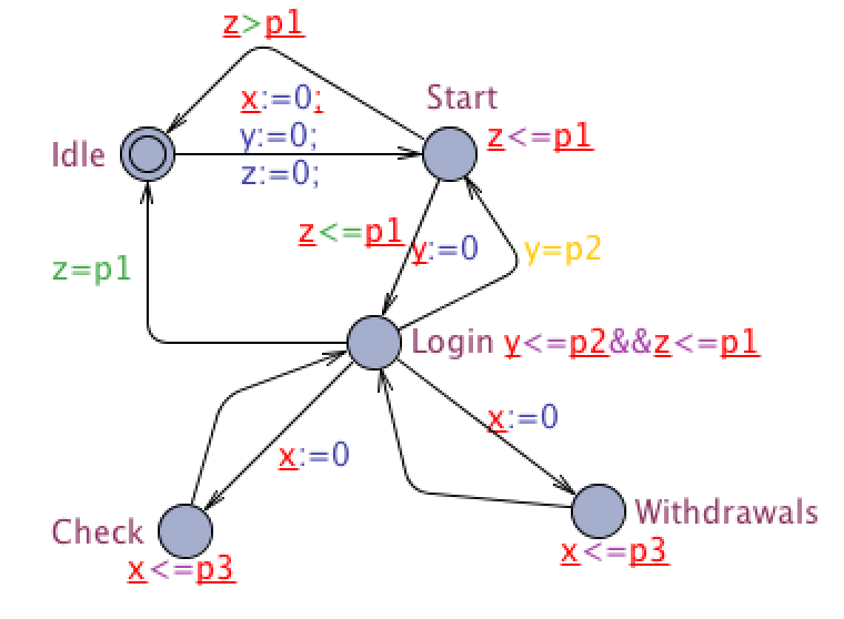
Figure 1: An ATM modeled using a PTA.

Example 1

The PTA in Fig. 1 models an ATM. It has 5 locations, 3 clocks $\{x,y,z\}$ and 3 parameters $\{p_{1},p_{2},p_{3}\}$. This PTA is deterministic and all the clocks are parametric. To understand the behavior of state transitions, for examples, the machine can initially idle for an arbitrarily long time. Then, the user can start the system by, say, pressing a button and the PTA enters location “Start” and resets the three clocks. The machine can remain in “Start” location as long as the invariant $z\leq p_{1}$ holds, and during this time the user can drive the system (by pressing a corresponding button) to login their account and the automaton enters location “Login” and resets clock $y$. A time-out action occurs and it goes back to “Idle” if the machine stays at “Start” for too long and the invariant $z\leq p_{1}$ becomes false. Similarly, the machine can remain in location “Login” as long as the invariant $y\leq p_{2}\wedge z\leq p_{1}$ holds and during this time the user can decide either to “Check” (her balance) or to “Withdraw” (money), say by pressing corresponding buttons. However, if the user does not take any of these actions $p_{2}$ time units after the machine enter location “Login”, the machine will back to “Start” location.

II-C Semantics of PTA via labeled transition systems

We use a standard model of labeled transition systems (LTS) for describing and analyzing the behavioral properties of PTA.

Definition 3 (LTS).

A labeled transition system (LTS) over a set of (action) symbols $\Delta$ is a triple $\mathcal{L}=(S,S_{0},\rightarrow)$, where

• $S$ is a set of states with a subset $S_{0}\subseteq S$ of states called the initial states.

• ${\rightarrow}\subseteq S\times\Delta\times S$ is a relation, called the transition relation.

We write $s\xrightarrow{a}s^{\prime}$ for a triple $(s,a,s^{\prime})\in{\rightarrow}$ and it is called a transition step by action $a$.

A run of $\mathcal{L}$ is a finite alternating sequence of states in $S$ and actions $\Delta$, $\xi=s_{0}a_{1}s_{1}\ldots a_{\ell}s_{\ell}$, such that $s_{0}\in S_{0}$ and $s_{i-1}\xrightarrow{a_{i}}s_{i}\in\rightarrow$ for $i=1,\ldots,\ell$. A run $\xi$ can be written in the form of $s_{0}\xrightarrow{a_{1}}s_{1}\xrightarrow{a_{2}}\cdots\xrightarrow{a_{\ell}}s_{\ell}$.

The length of a run $\xi$ is its number $\ell$ of transitions steps and it is denoted as $|\xi|$, and a state $s\in S$ is called reachable in $\mathcal{L}$ if $s$ is the last state a run of $\mathcal{L}$, e.g. $s_{\ell}$ of $\xi$.

Definition 4 (LTS semantics of PTA).

For a PTA $\mathcal{A}=(\Sigma,Q,q_{0},I,\rightarrow)$ and a parameter valuation $\gamma$, the concrete semantics of PTA under $\gamma$, denoted by $\mathcal{A}[\gamma]$, is the LTS $(S,S_{0},\rightarrow)$ over $\Sigma\cup\mathbb{R}^{+}$, where

• a state in $S$ is a location $q$ of $\mathcal{A}$ augmented with the clock valuations which together with the parameter valuation $\gamma$ satisfy the invariant $I_{q}$ of the location, that is

  $$S=\{(q,\omega)\in Q\times(X\rightarrow\mathbb{R}^{+})\mid(\gamma,\omega)\models I_{q}\}$$

  $$S_{0}=\{(q_{0},\omega)\mid(\gamma,\omega)\models I_{q_{0}}\wedge\omega=(0,\cdots,0)\}$$

• any transition step in the transition $\rightarrow$ of the LTS is either an instantaneous transition step by an action in $\Sigma$ defined by $\mathcal{A}$ or by a time advance, that are specified by the following rules, respectively

  • instantaneous transition: for any $a\in\Sigma$, $(q,\omega)\xrightarrow{a}(q^{\prime},\omega^{\prime})$ if there are simple constraint $g$ and an update set $u$ such that $q\xrightarrow{g\&a[u]}q^{\prime}$, $(\gamma,\omega)\models g$ and $\omega^{\prime}=\omega[u]$; and

  • time advance transition $(q,\omega)\xrightarrow{d}(q^{\prime},\omega^{\prime})$ if $q^{\prime}=q$ and $\omega^{\prime}=\omega+d$.

A concrete run of a PTA $\mathcal{A}$ for a given valuation $\gamma$ is a sequence of consecutive state transition steps $\xi=s_{0}\xrightarrow{t_{1}}s_{1}\xrightarrow{t_{2}}\cdots\xrightarrow{t_{\ell}}s_{\ell}$ of the LTS $\mathcal{A}[\gamma]$, which we also call a run of the LTS $\mathcal{A}[\gamma]$. A state $s=(q,\omega)$ of $\mathcal{A}[\gamma]$ is a reachable state of $\mathcal{A}[\gamma]$ if there exists some run $\xi=s_{0}\xrightarrow{t_{1}}s_{1}\xrightarrow{t_{2}}\cdots\xrightarrow{t_{\ell}}s_{\ell}$ of $\mathcal{A}[\gamma]$ such that $s=s_{\ell}$.

Without the loss of generality, we merge any two consecutive time advance transitions respectively labelled by $d_{i}$ $d_{i+1}$ into a single time advance transition labels by $d_{i}+d_{i+1}$. We can further merger a consecutive pair $s\xrightarrow{d}s^{\prime}\xrightarrow{a}s^{\prime\prime}$ of a timed advance transition by $d$ and an instantaneous transition by an action $a$ in a run into a single observable transition step $s\xrightarrow{a}s^{\prime\prime}$. If we do this repeatedly until all time advance steps are eliminated, we obtain an untimed run of the PTA (and the LTS), and the sequence of actions in an untimed run is called a trace.

We call an untimed run $\xi=s_{0}\xrightarrow{a_{1}}s_{1}\cdots\xrightarrow{a_{\ell}}s_{\ell}$ a simple run if $\omega_{i}\geq\omega_{i-1}$ for $i=1,\cdots,\ell$, where $s_{i}=(q_{i},\omega_{i})$. It is easy to see that $\xi$ is a simple untimed run if each transition by $a_{i}$ does not have any clock reset in $\xi$.

Definition 5 (LTS of trace).

For a PTA $\mathcal{A}$ and a syntactic run

$$\tau=(q_{0}{,}I_{q_{0}})\xrightarrow{g_{1}\&a_{1}[u_{1}]}(q_{1}{,}I_{q_{1}}){\cdots}\xrightarrow{g_{\ell}{\&}a_{\ell}[u_{\ell}]}(q_{\ell}{,}I_{q_{\ell}})$$

we define the PTA $\mathcal{A}_{\tau}{=}(\Sigma_{\tau}{,}Q_{\tau}{,}q_{0,\tau}{,}I_{\tau},\rightarrow_{\tau})$, where

• $\Sigma_{\tau}=\{a_{i}\mid i=1,\cdots,\ell\}$,

• $Q_{\tau}=\{q_{0},\cdots,q_{\ell}\}$ and $q_{0,\tau}=q_{0}$,

• $I_{\tau}(i)=I_{q_{i}}$ for $i\in Q$, and

• $\rightarrow_{\tau}=\{(q_{i-1},g_{i},a_{i},u_{i},q_{i})\mid i=1,\cdots,\ell\}$.

Give a parameter valuation $\gamma$, the concrete semantics of $\tau$ under $\gamma$ is defined to be the LTS $\mathcal{A}_{\tau}[\gamma]$.

For a syntactic run

$$\tau=(q_{0}{,}I_{q_{0}})\xrightarrow{g_{1}\&a_{1}[u_{1}]}(q_{1}{,}I_{q_{1}}){\cdots}\xrightarrow{g_{\ell}{\&}a_{\ell}[u_{\ell}]}(q_{\ell}{,}I_{q_{\ell}})$$

We use $R(\mathcal{A}_{\tau}[\gamma])$ to denote the set of states $(q_{k},\omega_{k})$ of $\mathcal{A}_{\tau}[\gamma]$ such that the following is a untimed run of $\mathcal{A}_{\tau}[\gamma]$

$$(q_{0},\omega_{0})\xrightarrow{a_{1}}(q_{1},\omega_{1})\cdots\xrightarrow{a_{k}}(q_{k},\omega_{k})\cdots\xrightarrow{a_{\ell}}(q_{\ell},\omega_{\ell})$$

II-D Two decision problems for PTA

We first present the properties of PTAs which we consider in this paper.

Definition 6 (Properties).

A state and a property for a PTA are specified by a state predicate $\phi$ and a temporal formula $\psi$ defined by the following syntax, respectively: for $x,y\in X$, $e\in\mathcal{E}$ and $\prec\in\{<,\leq,=\}$ and $q$ is a location.

$$\begin{array}[]{lllll}\phi&::=&x\prec e\mid-x\prec e\mid x-y\prec e\mid\\ &&q\mid\neg\phi\mid\phi\wedge\phi\mid\phi\vee\phi\\ \psi&::=&\forall\Box\phi\mid\exists\Diamond\phi\end{array}$$

Let $\gamma$ be a parameter valuation and $\phi$ be state formula. We say $\mathcal{A}[\gamma]$ satisfies $\exists\Diamond\phi$, denoted by $\mathcal{A}[\gamma]\models\exists\Diamond\phi$, if there is a reachable state $s$ of $\mathcal{A}[\gamma]$ such that $\phi$ holds in state $s$. We call these properties reachability properties. Similarly, $\mathcal{A}[\gamma]$ satisfies $\forall\Box\phi$, denoted by $\mathcal{A}[\gamma]\models\forall\Box\phi$, if $\phi$ holds in all reachable states of $\mathcal{A}[\gamma]$. We call these properties safety properties. We can see that if $\mathcal{A}[\gamma]{\models}\exists\Diamond\phi$, there is an syntactic run $\tau$ such that there is a state in $R(\mathcal{A}_{\tau}[\gamma])$ satisfies $\phi$. In this case, we also say that the syntactic run $\tau$ satisfies $\phi$ under the parameter valuation $\gamma$. We denote it by $\tau[\gamma]\models\phi$.

We are now ready to present the formal statement of the parameter synthesis problem and the emptiness problem of PTA.

Problem 1 (The parameter synthesis problem).

Given a PTA $\mathcal{A}$ and a property $\psi$, compute the entire set $\Gamma(\mathcal{A},\psi)$ of parameter valuations such that $\mathcal{A}[\gamma]\models\psi$ for each $\gamma\in\Gamma(\mathcal{A},\psi)$.

Solutions to the problems are important in system plan and optimization design. Notice that when there are no parameters in $\mathcal{A}$, the problem is decidable in PSPACE [2]. This implies that if there are parameters in $\mathcal{A}$, the satisfaction problem $\mathcal{A}[\gamma]\models\psi$ is decidable in PSPACE for any given parameter valuation $\gamma$.

A special case of the synthesis problem is the emptiness problem, which is by itself very important and formulated below.

Problem 2 (Emptiness problem).

Given a PTA $\mathcal{A}$ and a property $\psi$, is there a parameter valuation $\gamma$ so that $\mathcal{A}[\gamma]\models\psi$?

This is equivalent to the problem of checking if the set $\Gamma(\mathcal{A},\psi)$ of feasible parameter valuations is empty.

Many safety verification problems can be reduced to the emptiness problem. We say that Problem 2 is a special case of Problem 1 because solving the latter for a PTA $\mathcal{A}$ and a property $\psi$ solves Problem 2.

It is known that the emptiness problem is decidable for a PTA with only one clock [3]. However, the problem becomes undecidable for PTAs with more than two clocks [3]. Significant progress could only be made in 2002 when the subclass of L/U PTA were proposed in [6] and the emptiness problem was proved to be decidable for these automata. In the following, we will extend these results and define some classes of PTAs for which we propose solutions to the parameter synthesis problem and the emptiness problem.

III Parameter synthesis of PTA with one parametric clock

In this section, we present our first contribution and the solution to the parameter synthesis problem of PTAs with one parametric clock $x$ and one parameter which we call one-one PTAs. A one-one PTA allows an arbitrarily number of concretely constrained clocks, and we denote a one-one PTA $\mathcal{A}$ with the parametric clock $x$ and parameter $p$ as $\mathcal{A}[x,p]$, and as $\mathcal{A}$ when there is no confusion. We use $\mathcal{A}[p=v]$ for the LTS (and the concrete PTA) under the valuation $p=v$. Our main theorem is that the entire set of feasible parameter valuations $\Gamma(\mathcal{A}[x,p],\psi)$ is computable for any one-one PTA $\mathcal{A}[x,p]$ and any property $\psi$ defined. The theorem is formally stated below.

Theorem 1 (Synthesisability of one-one PTA).

The set $\Gamma(\mathcal{A},\psi)$ of feasible parameter valuations is solvable for any one-one PTA $\mathcal{A}[x,p]$ and any property $\psi$.

The establishment and proof of this theorem involve a sequence of techniques to reduce the problem to computing the set of reachable states of an LTS. The major steps of reduction include

1. Reduce the problem of satisfaction of a property $\psi$, say in the form of $\exists\Diamond\phi$, by a syntactic run $\tau$ to a reachability problem. This is done by encoding the state property in $\psi$ as a conjunction of the invariant of a state.

2. Then we move the state invariants in a syntactic run out of the states and conjoin them to the guards of the corresponding transitions.

3. Construct feasible runs for a given syntactic run in order to reach a given location. This requires to define the notions of effect lower and effect upper bounds of guards of transitions, through which an lower bound of feasible parameter valuation is defined.

III-A Reduce satisfaction of system to reachability problem

We note that $\psi$ is either of the form $\exists\Diamond\phi$ or the dual form $\forall\Box\phi$, where $\phi$ is a state property. Therefore, we only need to consider the problem of computing the set $\Gamma(\mathcal{A},\psi)$ for the case when $\psi$ is a formula of the form $\exists\Diamond\phi$, i.e., there is a syntactic run $\tau$ such that $\tau[\gamma]\models\phi$ for every $\gamma\in\Gamma(\mathcal{A},\psi)$. Our idea is to reduce the problem of deciding $\mathcal{A}\models\psi$ to a reachability problem of an LTS by encoding the state property $\phi$ in $\exists\Diamond\phi$ into the guards of the transitions of $\mathcal{A}$.

Definition 7 (Encoding state property).

Let $\phi$ be a state formula and $q$ be a location. We definite $\alpha(\phi,q)$ as follows, where $\equiv$ is used to denote syntactic equality between formulas:

• $\alpha(\phi,q)\equiv\phi$ if $\phi\equiv x-y\prec e$, $\phi\equiv x\prec e$ or $\phi\equiv-x\prec e$, where $x$ and $y$ are clocks and $e$ is an expression.

• when $\phi$ is a location $q^{\prime}$, $\alpha(\phi,q^{\prime})\equiv true$ if $q^{\prime}$ is $q$ and $false$ otherwise.

• $\alpha$ preserves all Boolean connectives, that is $\alpha(\neg\phi_{1},q)\equiv\neg\alpha(\phi_{1},q)$, $\alpha(\phi_{1}\wedge\phi_{2},q)\equiv\alpha(\phi_{1},q)\wedge\alpha(\phi_{2},q)$, and $\alpha(\phi_{1}\vee\phi_{2},q)\equiv\alpha(\phi_{1},q)\vee\alpha(\phi_{2},q)$.

We can easily prove the following lemma.

Lemma 1.

Given a PTA $\mathcal{A}$, $\psi\equiv\exists\Diamond\phi$, and a syntactic run of $\mathcal{A}$

$$\tau=(q_{0},I_{q_{0}})\xrightarrow{g_{1}\&a_{1}[u_{1}]}(q_{1},I_{q_{1}}){\cdots}\xrightarrow{g_{\ell}\&a_{\ell}[u_{\ell}]}(q_{\ell},I_{q_{\ell}})$$

we overload the function notation $\alpha$ and define the encoded run $\alpha(\tau)$ to be

$$(q_{0},I_{q_{0}})\xrightarrow{g_{1}\&a_{1}[u_{1}]}(q_{1}{,}I_{q_{1}}){\cdots}\xrightarrow{g_{\ell}\&a_{\ell}[u_{\ell}]}(q_{\ell}{,}I_{q_{\ell}}{\wedge}\alpha(\phi{,}q_{\ell}))$$

Then $\tau$ satisfies $\psi$ under parameter valuation $\gamma$ if and only if $R(\mathcal{A}_{\alpha(\tau)}[\gamma])\neq\emptyset$.

Notice the term guard is slightly abused in the lemma as $\alpha(\phi,q_{\ell})$ may have disjunctions, and thus it may not be a simple constraint.

III-B Moving state invariants to guards of transitions

It is easy to see that both the invariant $I_{q}$ in the pre-state of the transition and the guard $g$ in a transition step $(q,I_{q})\xrightarrow{g\&a[u]}(q^{\prime},I_{q^{\prime}})$ are both enabling conditions for the transition to take place. Furthermore, the invariant $I_{q^{\prime}}$ in the post-state of a transition needs to be guaranteed by the set of clock resets $u$. Thus we can also understand this constraint as a guard condition for the transition to take place (the transition is not allowed to take place if the invariant of the post-state is false).

For a PTA $\mathcal{A}$ and a syntactic run

$$\tau=(q_{0},I_{q_{0}})\xrightarrow{g_{1}\&a_{1}[u_{1}]}(q_{1}{,}I_{q_{1}}){\cdots}\xrightarrow{g_{\ell}\&a_{\ell}[u_{\ell}]}(q_{\ell},I_{q_{\ell}}).$$

Let $\overline{g}_{i}=(g_{i}\wedge I_{q_{i-1}}\wedge I_{q_{i}}[u_{i}])$. We define $\beta(\tau)$ as

$$\begin{split}(q_{0},true)\xrightarrow{\overline{g}_{1}\&a_{1}[u_{1}]}(q_{1},true)\cdots\xrightarrow{\overline{g}_{\ell}\&a_{\ell}[u_{\ell}]}(q_{\ell},true)\end{split}$$

Lemma 2.

For a PTA $\mathcal{A}$, parameter valuation $\gamma$ and a syntactic run

$$\tau=(q_{0},I_{q_{0}})\xrightarrow{g_{1}\&a_{1}[u_{1}]}(q_{1}{,}I_{q_{1}}){\cdots}\xrightarrow{g_{\ell}\&a_{\ell}[u_{\ell}]}(q_{\ell},I_{q_{\ell}})$$

we have $(\gamma,(0,\cdots,0))\models I_{q_{0}}$ and $R(\mathcal{A}_{\beta(\tau)}[\gamma])\neq\emptyset$ if and only if $R(\mathcal{A}_{\tau}[\gamma])\neq\emptyset$.

Proof.

Assume $(\gamma,x=0)\models I_{q_{0}}$ and $R(\mathcal{A}_{\beta(\tau)}[\gamma])\neq\emptyset$. There is run $\xi$ of $\mathcal{A}_{\beta(\tau)}[\gamma]$ which is an alternating sequence of instantaneous and time advance transition steps

$$\xi=(q_{0}{,}\omega_{0})\xrightarrow{d_{0}}(q_{0}{,}\omega_{0}^{\prime})\xrightarrow{a_{1}}(q_{1}{,}\omega_{1})\cdots\xrightarrow{a_{\ell}}(q_{\ell}{,}\omega_{\ell})$$

such that $(\gamma,\omega_{i}^{\prime})\models g_{a_{i+1}}\wedge I_{q_{i}}\wedge I_{q_{i+1}}[u_{a_{i+1}}]$ and $\omega_{i+1}=\omega_{i}^{\prime}[u_{a_{i}}]$ for $i=0,\cdots,\ell-1$. Hence, by the definition of $\mathcal{A}_{\tau}[\gamma]$, $\xi$ is also a run of $\tau$ under $\gamma$, and thus $R(\mathcal{A}_{\tau}[\gamma])\neq\emptyset$.

For the “if” direction, assume there is $\xi$ as defined above which is a run of $\tau$ for the parameter valuation $\gamma$. Then by the definition of the concrete semantics, we have $(\gamma,x=0)\models I_{q_{0}}$, $(\gamma,\omega_{i}^{\prime})\models g_{a_{i+1}}\wedge I_{q_{i}}$ and $(\gamma,\omega_{i}^{\prime}[u_{a_{i+1}}])\models I_{q_{i+1}}$ for $i=0.\cdots,\ell-1$. In other words, $(\gamma,\omega_{i}^{\prime})\models I_{q_{i+1}}[u_{a_{i+1}}]$ for $i=0.\cdots,\ell-1$. Therefore, $(\gamma,(0,\cdots,0))\models I_{q_{0}}$ and $\xi$ is a run of $\beta(\tau)$ under $\gamma$, i.e., $R(\mathcal{A}_{\beta(\tau)}[\gamma])\neq\emptyset$. ∎

III-C Generating semantic runs from syntactic runs

We now define the notions of lower bound and upper bound of guards of transitions, and use them to construct feasible runs from syntactic runs.

For a PTA $\mathcal{A}$, we use $\textit{maxC}(\mathcal{A})$ to denote the maximum of the absolute values of the constant terms occurring in the linear expressions of $\mathcal{A}$, that is,

$$\textit{maxC}(\mathcal{A})\ \widehat{=}\ \textit{max}\{|\textit{con}(e)|\mid e\in\textit{expr}(\mathcal{A})\}.$$

For a property $\psi$, we use $\textit{maxV}(\psi)$ to denote the maximum of absolute value of the constants which occur in $\psi$, and we define the constant $C\ \widehat{=}\ 2\cdot\max\{\textit{maxC}({\mathcal{A}}),\textit{maxV}(\psi)\}+2$.

Lemma 3.

For a one-one PTA $\mathcal{A}[x,p]$, a constant $T\geq C$ and a syntactic trace $\tau=a_{1}\cdots a_{\ell}$ of $\mathcal{A}[x,p]$ such that $R(\mathcal{A}_{\tau}[p=T])\neq\emptyset$, assume that $-x\prec-e_{1}$ (or equivalently $x\succ e_{1}$) and $x\prec e_{2}$ are two conjuncts of the guard $a_{i}$ for some $i\in\{1,\ldots,\ell\}$. Then ${\tt cf}(e_{1},p)\leq{\tt cf}(e_{2},p)$.

Proof.

By contradiction.

1. For the parameter valuation $\gamma=\{p=T\}$, assume that the lemma does not hold, i.e. ${\tt cf}(e_{1},p)>{\tt cf}(e_{2},p)$.

2. We have ${\tt cf}(e_{1}-e_{2},p)>0$.

3. By the definition of $C$, $C>|\textit{con}(e_{1})|+|\textit{con}(e_{1})|$. Then because $T\geq C$, we have $T>|\textit{con}(e_{1})|+|\textit{con}(e_{1})|$.

4. Results 1)&3) imply $(e_{1}-e_{2})[\gamma]>0$.

5. However, because $R(\mathcal{A}_{\tau}[\gamma])\neq\emptyset$, we have a concrete untimed run of $\mathcal{A}_{\tau}[p=T]$

   $$(q_{0}{,}\omega_{0}){\xrightarrow{a_{1}}}(q_{1}{,}\omega_{1}){\cdots}(q_{i}{,}\omega_{i}){\xrightarrow{a_{i}}}(q_{i+1},\omega_{i+1}){\cdots}{\xrightarrow{a_{\ell}}}(q_{\ell}{,}\omega_{\ell})$$

   The guard of $a_{i}$ holds for $(p=T,\omega_{i})$. Thus, the two conjuncts of the guard of $a_{i}$ imply that $(e_{1}-e_{2})[\gamma]\leq 0$. This contradicts with the result 4).

∎

Corollary 1.

For a one-one PTA $\mathcal{A}[x,p]$, let $\tau=a_{1}\cdots a_{\ell}$ be a syntactic trace of $\mathcal{A}[x,p]$ such that there is $T\geq C$ for which $R(\mathcal{A}_{\tau}[p=T])\neq\emptyset$. Assume that for some $i$ and $j$ such that $0\leq i<j\leq\ell$, $-x\prec-e_{1}$ is a conjunct of the guard of $a_{i}$ and $x\prec e_{2}$ is a conjunct of the guard of $a_{j}$. Then, ${\tt cf}(e_{1},p)\leq{\tt cf}(e_{2},p)$ if the transitions $a_{k}$ for $k\in[i,j)$ do not reset any clock, i.e. their reset sets are empty.

Definition 8 (Order between lower and upper bound constraints).

For two lower bounds $x\succ_{1}e_{1}$ and $x\succ_{2}e_{2}$ such that $\succ_{1},\succ_{2}\in\{>,\geq\}$ and a parameter $p$, we define that the order $(x\succ_{1}e_{1})\sqsupseteq_{p}(x\succ_{2}e_{2})$ holds if one of the following conditions holds.

1. ${\tt cf}(e_{1},p)>{\tt cf}(e_{2},p)$;

2. ${\tt cf}(e_{1},p)={\tt cf}(e_{2},p)\wedge(\textit{con}(e_{1})>\textit{con}(e_{2}))$;

3. $e_{1}=e_{2}$ and $x\succ_{1}e_{1}\equiv x>e_{1}$;

4. $e_{1}=e_{2}$ and $x\succ_{2}e_{2}\equiv x\geq e_{2}$.

Symmetrically, let $x\prec_{1}e_{1}$ and $x\prec_{2}e_{2}$ be two upper bounds such that $\prec_{1},\prec_{2}\in\{<,\leq\}$. We define that $(x\prec_{1}e_{1})\sqsubseteq_{p}(x\prec_{2}e_{2})$ holds if one of the following conditions holds.

1. ${\tt cf}(e_{1},p)<{\tt cf}(e_{2},p)$;

2. ${\tt cf}(e_{1},p)={\tt cf}(e_{2},p)\wedge(\textit{con}(e_{1})<\textit{con}(e_{2}))$;

3. $e_{1}=e_{2}$ and $(x\prec_{1}e_{1})\equiv(x<e_{1})$;

4. $e_{1}=e_{2}$ and $(x\prec_{2}e_{2})\equiv(x\leq e_{2})$.

For a one-one PTA $\mathcal{A}[x,p]$, we define the effective lower bound of a guard $g$, denoted by ${\tt elb}(g,p)$, as a syntactic term

$${\tt elb}(g,p)\equiv\left\{\begin{array}[]{llll}x>-1&\mbox{no lower bound $x\succ e$ occurs in $g$}\\ x\succ_{1}e&\mbox{if }x\succ_{1}e\mbox{ is one conjunct of }\\ &g\mbox{ and for all $x\succ_{2}e_{1}$ in $g$,}\\ &\mbox{$(x\succ_{1}e)\sqsupseteq_{p}(x\succ_{2}e_{1})$}\end{array}\right.$$

Symmetrically, we define the effective upper bound of a guard $g$

$${\tt eup}(g,p)\equiv\left\{\begin{array}[]{llll}x<\infty&\mbox{no upper bound $x\prec e$ in $g$}\\ x\prec_{1}e&\mbox{if }x\prec_{1}e\mbox{ is one conjunct of }g\\ &\mbox{and for all $x\prec_{2}e_{1}$ in $g$,}\\ &\mbox{$(x\prec_{1}e)\sqsubseteq_{p}(x\prec_{2}e_{1})$}\end{array}\right.$$

Lemma 4.

Let $\mathcal{A}[x,q]$ be a one-one PTA and

$$\tau=q_{0}\xrightarrow{g_{1}\&a_{1}}q_{1}\cdots\xrightarrow{g_{\ell}\&a_{\ell}}q_{\ell}$$

a syntactic run which has no invariants for the locations and no reret sets for the actions.

If there is a $T\geq C$ such that $R(\mathcal{A}_{\tau}[p=T])\neq\emptyset$, ${\tt elb}(g_{i},p)\wedge{\tt eup}(g_{j},p)$ holds for each valuation $p=t$ such that $t\in[C,\infty)$, where $g_{i}$ and $g_{j}$ are the guards of $a_{i}$ and $a_{j}$ for $i,j\in\{1,\ldots,\ell\}$ such that $i\leq j$, respectively.

Proof.

Assume $R(\mathcal{A}_{\tau}[p=T])\neq\emptyset$. Then there is a concrete run of $\mathcal{A}_{\tau}[p=T]$

$$\xi=(q_{0},\omega_{0})\xrightarrow{a_{1}}(q_{1},\omega_{1})\cdots\xrightarrow{a_{\ell}}(q_{\ell},\omega_{\ell})$$

Since for all $i,j\in\{1,\ldots,\ell\}$, the transition by $a_{i}$ does not reset the clock $x$, $\omega_{i}(x)\leq\omega_{j}(x)$ if $i\leq j$. Let us set ${\tt eup}(g_{i},p)\equiv x\prec_{i}e_{i}$ and ${\tt elb}(g_{j},p)\equiv x\succ_{j}e_{j}$. Since $\omega_{i}(x)\leq\omega_{j}(x)$, we have

• if $\prec_{i}$ is $<$, $e_{i}[p=T]<e_{j}[p=T]$, else

• if $\succ_{j}$ is $>$, $e_{i}[p=T]<e_{j}[p=T]$, else

• $e_{i}[p=T]\leq e_{j}[p=T]$.

We now make the following two claims:

1. if $e_{i}[p=T]<e_{j}[p=T]$, $e_{i}[p=T^{\prime}]<e_{j}[p=T^{\prime}]$ for $T^{\prime}\in[C,\infty)$; and

2. if $e_{i}[p=T]\leq e_{j}[p=T]$, $e_{i}[p=T^{\prime\prime}]\leq e_{j}[p=T^{\prime\prime}]$ for $T^{\prime\prime}\in[C,\infty)$. We prove these two claims below.

We prove these two claims as follows.

1. In the case when $e_{i}[p=T]<e_{j}[p=T]$, we have ${\tt cf}({\tt elb}(g_{i},p),p)\leq{\tt cf}({\tt eup}(g_{j},p),p)$ according to Corollary 1. Hence, ${\tt cf}(e_{j}-e_{i},p)\geq 0$. In case when ${\tt cf}(e_{i}-e_{j},p)=0$, $e_{i}[p=T^{\prime}]<e_{j}[p=T^{\prime}]$ for $T^{\prime}\in[C,\infty)$. If ${\tt cf}(e_{j}-e_{i},p)>0$, $(e_{j}-e_{i})[p=T^{\prime}]\geq T^{\prime}-|con(e_{i})|-|con(e_{i})|>0$ for $T^{\prime}\in[C,\infty)$. Hence, Claim 1) holds.

2. The proof for Claim 2) in the case when $e_{i}[p=T]\leq e_{j}[p=T]$, is the same.

Based on these claims, we prove that for $T^{\prime}\in[C,\infty)$.

• if $\prec_{i}$ is the relation $<$, $e_{i}[p=T^{\prime}]>e_{j}[p=T^{\prime}]$, else

• if $\succ_{j}$ is the relation $>$, $e_{i}[p=T^{\prime}]>e_{j}[p=T^{\prime}]$, else

• $e_{i}[p=T^{\prime}]\geq e_{j}[p=T^{\prime}]$.

Therefore, formula ${\tt elb}(g_{i},p)\wedge{\tt eup}(g_{j},p)$ is feasible for $T^{\prime}\in[C,\infty)$. ∎

Definition 9 (From syntactic to feasible timed run).

For a guard, we define

$${\tt\theta}(g,T)\ \widehat{=}\ \left\{\begin{array}[]{@{}ll@{}}max\{0,e[p=T]\},\mbox{ if }{\tt elb}(g,p)\equiv x\geq e\\ max\{0,e[p=T]+1\},\mbox{ if }{\tt elb}(g,p)\equiv x>e\end{array}\right.$$

Given a simple syntactic run which have no location invariants and clock resets $\tau=q_{0}\xrightarrow{g_{1}\&a_{1}}q_{1}\cdots\xrightarrow{g_{\ell}\&a_{\ell}}q_{\ell}$, let

$${\tt\Theta}(\tau,T)\ \widehat{=}\ (q_{0},w_{0})\xrightarrow{a_{1}}(q_{1},\omega_{1})\cdots\xrightarrow{a_{\ell}}(q_{\ell},\omega_{\ell})$$

such that

$$\omega_{i}=\left\{\begin{array}[]{@{}ll@{}}0,&\mbox{if }i=0,\\ {\tt\theta}(g,T),&\mbox{otherwise}.\end{array}\right.$$

We now provide Algorithm 1 for the generation of a feasible timed run from a simple syntactic run.

1

input :  A simple syntactic run of $\mathcal{A}[x,p]$ $\tau=q_{0}a_{1}q_{1}\cdots a_{\ell}q_{\ell}$ such that there is a $T_{1}\geq C$ and $R(\tau[p=T_{1}])\neq\emptyset$; an integer $T\geq C$.

output :  A run $\xi=s_{0}d_{0}s_{0}^{\prime}a_{1}s_{1}\cdots d_{\ell-1}s_{\ell-1}^{\prime}a_{\ell}s_{\ell}$ is a run of $\mathcal{A}[p=T]$.

2

3Set $s_{0}a_{1}s_{1}\cdots a_{\ell}s_{\ell}={\tt\Theta}(\tau,T)$ where $s_{i}=(q_{i},\omega_{i})$

4 Set $\xi_{1}=s_{0}a_{1}s_{1}\cdots a_{\ell}s_{\ell}$

5 while $\xi_{2}$ is not a simple feasible sequence do

6       for  $i\in[1,\ell]$  do

7             if  $\omega_{i}<\omega_{i-1}$ then

8                   Set $\omega_{i}=\omega_{i-1}$;

9             end if

10            

11       end for

12      

13 end while

14for  $i\in[1,\ell]$  do

15       $d_{i-1}=\omega_{i}-\omega_{i-1}$; $s_{i-1}^{\prime}=(q_{i-1},\omega_{i})$;

16 end for

17return $s_{0}d_{0}s_{0}^{\prime}a_{1}s_{1}\cdots d_{\ell-1}s_{\ell-1}^{\prime}a_{\ell}s_{\ell}$

Algorithm 1 GSR (Generate Simple Feasible Run)

Lemma 5.

Algorithm 1 terminates within a finite number of steps. When it terminates, $(p=T,\omega_{i})\models g_{i}$ holds for the output $\xi=s_{0}d_{0}s_{0}^{\prime}a_{1}s_{1}\cdots d_{\ell-1}s_{\ell-1}^{\prime}a_{\ell}s_{\ell}$, where $g_{i}$ is the guard of transition $a_{i}$ for $i=1,\cdots,\ell$.

Proof.

To prove the termination, let $M=\max\{w_{i}\mid i=0,\cdots,\ell\}$. It is easy to see that $(\omega_{0}\leq M\wedge\cdots,\omega_{\ell}\leq M)$ is an invariant of the while loop, i.e. it holds when the execution enters line 1. Each iteration of the loop body increase at least one of $\omega_{i}$ by the execution of the statement of line 1. Hence, the algorithm terminates within a finite number of iterations, as otherwise the invariant would be falsified.

We prove the correctness of the algorithm by contradiction. Assume that there is an $i\in\{1,\ldots,\ell\}$ such that $(p=T,\omega_{i})\not\models g_{i}$. By the definition of ${\tt\Theta}(\tau,T)$, $(T,\omega_{i})\models g_{i}$ holds after the execution of the statement in line 1 of Algorithm 1.

It is noticed that $\omega_{i}$ is possibly changed only by the statement $\omega_{i}:=\omega_{i-1}$ in line 1, which increases $\omega_{i}$. Therefore, when the algorithm terminates for any $i\in\{1,\ldots,\ell\}$, $\omega_{i}=\omega_{k}^{0}$ for some $k\leq i$, where $\omega_{k}^{0}$ is the initial value of $\omega_{k}$. Assume $(T,\omega_{i})\models g_{i}$ does not hold, that is, $(T,\omega_{i})\not\models g_{i}$ holds. This implies that $(T,\omega_{i})\not\models{\tt eup}(g_{i},p)$. By the definition of ${\tt\theta}(g_{k},T)$, ${\tt\theta}(g_{k},T)=\omega_{k}^{0}$ is the minimum value of $x$ which make formula $(T,x)\models g_{k}$ hold. According to Lemma 4, formula ${\tt elb}(g_{k},p)\wedge{\tt eup}(g_{i},p)$ is feasible for $p\in[C,\infty)$. Because ${\tt eup}(g_{i},p)$ is an upper bound constraint and $\omega_{i}=\omega_{k}^{0}$, $(T,\omega_{i})\models{\tt elb}(g_{k},p)\wedge{\tt eup}(g_{i},p)$. Which contradicts with the assumption that $(T,\omega_{i})\models{\tt eup}(g_{i},p)$ does not hold. Therefore $(T,\omega_{i})\models{\tt eup}(g_{i},p)$ must hold. This implies $(T,\omega_{i})\models g_{i}$ holds for $i=1,\cdots,\ell$. ∎

Lemma 6.

Let $\tau$ be a simple syntactic run of a one-one PTA $\mathcal{A}[x,p]$. We have $R(\mathcal{A}_{\tau}[p=T])\neq\emptyset$ for any $T\geq C$ if there is a $T_{1}\geq C$ such that $R(\mathcal{A}_{\tau}[p=T_{1}])\neq\emptyset$.

Proof.

Algorithm 1 generates a run of $\mathcal{A}_{\tau}[p=T]$ for simple syntactic run $\tau$. ∎

Lemma 7.

Let $\mathcal{A}[x,p]$ be a one-one PTA and $\psi$ a formula of the form $\exists\Diamond\phi$. Then, $\mathcal{A}[p=T]\models\psi$ for all $T\geq C$ if there is a $T_{1}\geq C$ such that $\mathcal{A}[p=T_{1}]\models\psi$,.

Proof.

For the parameter valuation $\gamma=\{p=T_{1}\}$, let $\phi=q_{\ell}$ without the loss of generality, as the proof will be similar when $\phi$ is in other forms. Assume $\mathcal{A}[p=T_{1}]\models\psi$, we need to prove that $\mathcal{A}[p=T]\models\psi$ for any $T\geq C$.

Let $\tau=q_{0}\xrightarrow{a_{1}}q_{1}\cdots\xrightarrow{a_{\ell}}q_{\ell}$ be a syntactic run of $\mathcal{A}[p=T_{1}]$ that satisfies property $\psi$, i.e. $R(\mathcal{A}_{\tau}[p=T])\neq\emptyset$. According to Lemma 2, we obtain an untimed run $\beta(\tau)$ without location invariant which satisfies that $R(\mathcal{A}_{\beta(\tau)}[p=T_{1}])\neq\emptyset$ if and only if $R(\mathcal{A}_{\tau}[p=T_{1}])\neq\emptyset$. Without the loss of generality, set

$$\beta(\tau)=q_{0}\xrightarrow{g_{1}\&a_{1}[u_{1}]}q_{1}\cdots\xrightarrow{g_{\ell}\&a_{\ell}[u_{\ell}]}q_{\ell}.$$

Let $k$ be the number of transitions in $\beta(\tau)$ which reset the clock $x$. We prove the lemma by induction on $k$.

For $k=0$, $\beta(\tau)$ is a simple untimed run and $R(\mathcal{A}_{\beta(\tau)}[p=T])\neq\emptyset$ follows from Lemma 6.

We assume $R(\mathcal{A}_{\tau}[p=T])\neq\emptyset$ holds for $k_{0}$ and let $k=k_{0}+1$. Assume $a_{i}$ is the action for the last transition in $\beta(\tau)$ that resets the clock $x$, and let

$$\tau_{2}=q_{0}\xrightarrow{g_{1}\&a_{1}[u_{1}]}q_{1}\cdots\xrightarrow{g_{i}\&a_{i}[u_{i}]}q_{i}$$

We obtain the sequence $\tau_{2}^{\prime}$

$$\tau_{2}^{\prime}=q_{0}\xrightarrow{g_{1}\&a_{1}[u_{1}]}q_{1}\cdots\xrightarrow{g_{i}\&a_{i}}q_{i}$$

by removing the last reset set $u_{i}$ of $\tau_{2}$.

By the induction hypothesis and $\tau_{2}^{\prime}$ has $k_{0}$ transitions that modify $x$, $R(\mathcal{A}_{\tau_{2}^{\prime}}[p=T])\neq\emptyset$ for any $T\geq C$. Since $\tau_{2}^{\prime}$ is the same as $\tau_{2}^{\prime}$ excpet the reset set of last transition, $R(\mathcal{A}_{\tau_{2}}[p=T])\neq\emptyset$ for any $T\geq C$. The value of clock $x$ is a fixed value when the run reaches $q_{i}$ in $\tau_{2}$, sine there is a reset of $x$ in transition $a_{i}$. And this value is the same as the value of clock $x$ when the run reaches $q_{i}$ in the run $\beta(\tau)$ under the parameter valuation $p=T_{1}$. As there is no reset of $x$ in transitions $a_{i+1},\cdots,a_{\ell}$. Hence, $R(\mathcal{A}_{\beta({\tau})}[p=T])\neq\emptyset$ for $T\geq C$.

∎

III-D The proof of the main theorem

We can now prove Theorem 1 of this section.

Proof.

Assume that $\mathcal{A}[p=C]\models\psi$. Following Lemma 7, we initially start with the subset of parameter valuations $H=\{C,C+1,\cdots\}\subseteq\Gamma(\mathcal{A},\psi)$. We then iteratively check if $\mathcal{A}[p=i]\models\psi$ holds for $i=0.\cdots,C-1$ and add to $H$ those $i$’s such that $\mathcal{A}[p=i]\models\psi$ holds. This procedure terminates with $H=\Gamma(\mathcal{A},\psi)$. ∎

Corollary 2.

Let $\mathcal{A}[x,p]$ be a one-one PTA . The set $\Gamma(\mathcal{A},\psi)$ is solvable if $\psi$ is the form $\forall\Box\phi$.

IV Parameter synthesis problem for L/U-automata

In this section, we will consider the parameter synthesis problem of L/U-automata which defined in [6] as given below.

Definition 10 (L/U automata).

Let $e=c_{0}+c_{1}p_{1}+\cdots+c_{n}p_{n}$ be a linear expression. For $i=1,\cdots,n$, we say $p_{i}$ occurs in $e$ if $c_{i}\neq 0$, occurs positive in $e$ if $c_{i}>0$, and occurs negative in $e$ if $c_{i}<0$.

• A parameter $p$ of PTA $\mathcal{A}$ is a lower bound (or an upper-bound) parameter if it only occurs negative (resp. positive) in the expressions of $\mathcal{A}$.

• $\mathcal{A}$ is called a lower-bound/upper-bound (L/U) automaton if every parameter of $\mathcal{A}$ is either a lower-bound parameter or an upper-bound parameter.

For instance, $p_{1}$ is an upper bound parameter in $x-y<2p_{1}$; $p_{2}$ and $p_{3}$ are lower bound parameters in $y-x<-p_{2}-3p_{3}$ and in $x-y<2p_{1}-p_{2}-2p_{3}$. A PTA which contains both the constraints $x-y\leq p_{1}-p_{2}$ and $z<p_{2}-p_{1}$ is not an L/U automaton.

IV-A Parameter synthesis for L/U-automata

Clearly, the parameters in a PTA $\mathcal{A}$ can be divided into two $L(\mathcal{A})$ and $U(\mathcal{A})$ which are the sets lower-bound parameters and upper-bound parameters, respectively. For a parameter valuation $\gamma$ we use $\gamma_{l}$ and $\gamma_{u}$ to denote its restrictions on $L$ and $U$, respectively. The following proposition in [6] is useful for us.

Proposition 1.

Let $\mathcal{A}$ be an L/U automaton and $\phi$ a state formula. Then

1. $\mathcal{A}[\gamma_{l}{,}\gamma_{u}]{\models}\exists\Diamond\phi$ iff $\forall\gamma_{l}^{\prime}{<}\gamma_{l}{,}\gamma_{u}{<}\gamma_{u}^{\prime}{:}\mathcal{A}[\gamma_{l}^{\prime}{,}\gamma_{u}^{\prime}]{\models}\exists\Diamond\phi$.

2. $\mathcal{A}[\gamma_{l}{,}\gamma_{u}]{\models}\forall\Box\phi$ iff $\forall\gamma_{l}{<}\gamma_{l}^{\prime}{,}\gamma_{u}^{\prime}{<}\gamma_{u}{:}\mathcal{A}[\gamma_{l}^{\prime}{,}\gamma_{u}^{\prime}]{\models}\forall\Box\phi$.

The proof of this proposition given in [6] needs to extend the notion of a parameter valuation to that of a partial parameter valuation which allow a parameter to be “undefined”. We use $\infty$ to denote the undefined value. Thus, a partial valuation $\gamma$ assigns a parameter with a value in ${\mathbb{N}}\cup\{\infty\}$, rather than in ${\mathbb{N}}$ only.

Partial parameter valuations are useful in certain cases to solve the verification problem. However partial parameter valuations may cause problems. For example, if $\gamma[p_{1}]=\gamma[p_{2}]=\infty$, what would be the value of $\gamma(e_{1}-e_{2})$? To avoid this problem, we require that a partial parameter valuation does not assign $\infty$ to both a lower-bound parameter and an upper-bound parameter. Also we follow the conventions that the truth values of $0\cdot\infty=0$, and $x-y\prec\infty$ are true and the truth value of $x-y\prec-\infty$ is false. We use $[0,\infty]$ to denote the valuation which assigns $0$ for each lower bound parameter and $\infty$ to each upper bound parameter.

We now show that the emptiness problem of an L/U automaton can be reduced to the reachability problem of its corresponding timed automaton under parameter valuation $[0,\infty]$.

Proposition 2.

Let $\mathcal{A}$ be an L/U automaton and $\phi$ be a state formula. Then $\mathcal{A}[0,\infty]\models\exists\Diamond\phi$ if and only if there exists a parameter valuation and clock evaluation $\omega$ such that $\mathcal{A}[\gamma,\omega]\models\exists\Diamond\phi$.

Proof.

The “if” part is an immediate consequence of Proposition 1. For the “only if” part, assume that $\xi$ is a run of $\mathcal{A}[0,\infty]$ which satisfies $\phi$. Let $T$ the maximum clock value occurring in $\xi$ and $T^{\prime}$ be the smallest constant occurring in $\mathcal{A}$ and $\phi$. More precisely, if $\xi=(q_{0}{,}\omega_{0}){\xrightarrow{a_{1}}}(q_{1}{,}\omega_{1}){\xrightarrow{a_{2}}}{\cdots}{\xrightarrow{a_{\ell}}}(q_{\ell}{,}\omega_{\ell})$, then $T=\max\{\omega_{i}(x)~{}|~{}0\leq i\leq\ell,x\in X\}$. Let $\gamma_{l}(p)=0$ for $p\in L$ and $\gamma_{u}(p)=T+|T^{\prime}|+1$ for $p\in U$. The proposition can then be proven by considering the different possible cases of the location invariants and guards of the transitions in $\xi$. For example, assume $g=x-y\prec e$ is the invariant of a location location $q_{i}$, or a conjunct of the guard of transition by $a_{i}$, or a conjunct of $\phi$. The relation $\omega_{i}(x)-\omega_{i}(y)\prec e[\gamma_{l},\gamma_{u}]$ holds for the definition of $\gamma_{l}$ and $\gamma_{u}$. Hence, $((\gamma_{l},\gamma_{u}),\omega_{i})\models g$. Thus, $\xi$ is a run of $\mathcal{A}[\gamma_{l},\gamma_{u}]$ and $\mathcal{A}[\gamma_{l},\gamma_{u}]\models\exists\Diamond\phi$. ∎

Proposition 2 provides an algorithm to check the satisfaction of a property with existential quantifiers by an L/U-automaton. Base on the “monotonic” property of L/U-automata, this actually reduces the emptiness problem an L/U-automaton to the reachable problem of corresponding timed automaton.

Lemma 8.

For a one-one L/U PTA $\mathcal{A}[x,p]$ and a formula $\psi\equiv\exists\Diamond\phi$, if there exists $T\geq C$ such that $\mathcal{A}[p=T]\models\psi$, then set $\Gamma(\mathcal{A},\psi)$ is computable.

Proof.

Suppose there is a syntactic run

$$\tau=(q_{0},I_{q_{0}})\xrightarrow{g_{1}\&a_{1}[u_{1}]}(q_{1},I_{q_{1}})\cdots\xrightarrow{g_{\ell}\&a_{\ell}[u_{\ell}]}(q_{\ell},I_{q_{\ell}})$$

which satisfies $\psi$ under the parameter valuation $p=T$. According Lemma 7, $\mathcal{A}[p=T_{1}]\models\psi$, for $T_{1}\geq C$. Then, we can check wether $\mathcal{A}[p=T_{1}]\models\psi$ for $T_{1}\in[0,C]$. Therefore, set $\Gamma(\mathcal{A},\psi)$ is computable.

∎

Proposition 3.

For a one-one L/U automaton $\mathcal{A}[x,p]$ and state property $\psi$, the set $\Gamma(\mathcal{A},\psi)$ is computable for $\psi\equiv\exists\Diamond\phi$.

Proof.

Let $H$ be $\Gamma(\mathcal{A},\psi)$. Assume that $p$ is a lower bound parameter. First check whether $\mathcal{A}[p=0]\models\psi$ hold or not. Since $\mathcal{A}[p=0]$ is a timed automaton, this checking is decidable. If $\mathcal{A}[p=0]\models\psi$ does not hold, then employ Proposition 2, $H=\emptyset$. Otherwise, if $\mathcal{A}[p=C]\models\psi$ does not hold, then employ Lemma 8, $H\subseteq\{0,1,\cdots,C-1\}$. We can check whether $\mathcal{A}[p=i]\models\psi$ holds or not from $i=C-1$ to $i=0$ until formula holds, then $H=\{0,\cdots,i\}$. If $\mathcal{A}[p=C]\models\psi$ holds, $H$ is solvable follows from Lemma 8.

If $p$ is an upper parameter. First check whether $\mathcal{A}[p=\infty]\models\psi$ holds or not. Since $\mathcal{A}[p=\infty]$ is a timed automaton, this checking is decidable. If $\mathcal{A}[p=\infty]\models\psi$ does not hold, $H=\emptyset$ follows from Proposition 2. Otherwise, assuming that $\xi$ is a run of $\mathcal{A}[0,\infty]$ that satisfies $\phi$. Let $T^{\prime}$ be the smallest constant occurring in $\mathcal{A}$ and $\phi$. And let $T$ be the maximum clock value occurring in $\xi$. More precisely, if $\xi=s_{0}\xrightarrow{a_{1}}s_{1}\cdots\xrightarrow{a_{\ell}}s_{\ell}$ and $s_{i}=(q_{i},\omega_{i})$, then $T=\max_{i\leq\ell,x\in X}\omega_{i}(x)$ It is easy to check that $\{T+|T^{\prime}|+1,\infty\}\subseteq H$. We iteratively check whether $\mathcal{A}[p=i]\models\psi$ holds or not from $i=0$ to $i=T+|T^{\prime}|+1$ until formula holds, then $H=\{i,i+1,\cdots,\infty\}$.

∎

For an L/U automaton $\mathcal{A}$ with one parameter $p$ and a property $\psi$, the work in [7] shows that the complexity of computing $\Gamma(\mathcal{A},\psi)$ is PSPACE-complete.

Corollary 3.

For a one-one L/U PTA $\mathcal{A}[x,p]$ and state property $\psi$, the set $\Gamma(\mathcal{A},\psi)$ is computable for $\psi=\forall\Box\phi$.

Proof.

Let $H$ be $\Gamma(\mathcal{A},\psi)$ and $H_{1}$ the set of parameter valuations which make $\mathcal{A}[\gamma]\models\exists\Diamond\neg\phi$ hold. It is easy to know that ${\mathbb{N}}=H\cup H_{1}$ and $H\cap H_{1}=\emptyset$. By Proposition 3, $H_{1}$ is computable, hence $H={\mathbb{N}}\setminus H_{1}$ is also computable. ∎

Theorem 2.

For a L/U PTA $\mathcal{A}$ with one parametrically constrained clock, the set $\Gamma(\mathcal{A},\psi)$ is computable if $\psi\equiv\exists\Diamond\phi$ and all the parameters are lower bound parameter or all the parameters are upper bound parameter.

Proof.

Let $H=\Gamma(\mathcal{A},\psi)$. If all the parameters are lower bound parameter, we construct a PTA $\mathcal{A}^{\prime}$ from $\mathcal{A}$ by replacing all the parameters of $\mathcal{A}$ by the single parameter $p$. Then $\mathcal{A}^{\prime}$ is be an L/U automaton with one parameter $p$. Employing Proposition 3, we can compute a set $H^{\prime}=\Gamma(\mathcal{A}^{\prime},\psi)$. When $H^{\prime}=\emptyset$, by Proposition 1, $(0,\cdots,0)\in H$ if $H\neq\emptyset$. Hence $H=\emptyset$. When $H^{\prime}={\mathbb{N}}$, i.e., after setting each parameter of $\mathcal{A}$ to $\infty$, $\psi$ also holds. Hence, $H={\mathbb{N}}^{m}$. Otherwise, by the Proposition 3, there is a $T\geq 0$ such that $H^{\prime}=\{0,1\cdots,T\}$. Assuming that there is parameter valuation $\gamma$ such that $\gamma(p_{i})\geq T+1$ for all $i=1,\cdots,m$ such that $\mathcal{A}[\gamma]\models\psi$, by the Proposition 1, $(T+1,\cdots,T+1)\in H$ and $T+1\in H^{\prime}$, which contracts with $H^{\prime}=\{0,\cdots,T\}$. Hence, the assumption does not hold and there exits at least one component of $\gamma$ which less or equal than $T$ for each $\gamma\in H$. Let $\mathcal{A}^{\prime}_{ij}$ be a PTA which obtain from set parameter $p_{i}$ to $j$. Let $H^{\prime}_{ij}$ be set of parameter valuation such that $\mathcal{A}_{ij}^{\prime}[\gamma]\models\psi$. We lift $H_{i,j}^{\prime}$ to $H_{i,j}$ by let the $i$-th of $H_{i,j}$ be $j$ and other components be the same as $H_{i,j}^{\prime}$. In other words,

$$H_{ij}=\{\gamma\mid\left(\gamma[p]=\gamma_{1}[p],p\neq p_{i}\right)\wedge\left(\gamma(p_{i})=j\right),\gamma_{1}\in H_{ij}^{\prime}\}.$$

Then $H=\bigcup_{i=1}^{m}\bigcup_{j=0}^{T}H_{ij}$.

If all the parameters are upper bound parameter, we construct a PTA $\mathcal{A}^{\prime}$ from $\mathcal{A}$ by replacing all the parameters of $\mathcal{A}$ by the single parameter $p$. Then $\mathcal{A}^{\prime}$ is an L/U automaton with one parameter. Let $H^{\prime}$ be $\Gamma(\mathcal{A}^{\prime},\psi)$. Following Proposition 3, we can compute $H^{\prime}$. When $H^{\prime}=\emptyset$. From Proposition 1, $(\sum_{i=1}^{m}\gamma(p_{i}),\cdots,\sum_{i=1}^{m}\gamma(p_{i}))\in H^{\prime}$ for each $\gamma\in H$. Hence $H=\emptyset$. When $H^{\prime}={\mathbb{N}}$, in the other words, after setting each parameter of $\mathcal{A}$ to $0$, $\mathcal{A}[p=0]\models\psi$ also holds. Hence, $H={\mathbb{N}}^{m}$. If $H^{\prime}\neq$ and $H^{\prime}\neq{\mathbb{N}}$, by the Proposition 3, there is a $T>0$ such that $H^{\prime}=\{T,T+1,\cdots,\infty\}$. By the definition of $H^{\prime}$, $(T,\cdots,T)\in H$, therefore, $\{\gamma\mid\gamma(p_{i})\geq T,i=1,\cdots,m\}\subseteq H$. Let $\mathcal{A}^{\prime}_{ij}$ be a PTA which obtain from set parameter $p_{i}$ by $j$. Let $H^{\prime}_{ij}$ be $\Gamma(\mathcal{A}^{\prime}_{ij},\psi)$. We lift $H_{i,j}^{\prime}$ to $H_{i,j}$ by

$$H_{ij}=\{\gamma\mid\left(\gamma[p]=\gamma_{1}[p],p\neq p_{i}\right)\wedge\left(\gamma(p_{i})=j\right),\gamma_{1}\in H_{ij}^{\prime}\}.$$

Then $H=\left(\bigcup_{i=1}^{m}\bigcup_{j=0}^{T-1}H_{ij}\right)\cup\{\gamma\mid\gamma(p_{i})\geq T,i=1,\cdots,m\}$, since there is at least one component of $\gamma$ less than $T$ excpet $\{\gamma\mid\gamma(p_{i})\geq T,i=1,\cdots,m\}$.

∎

Remark 1.

When all the parameters are lower-bound parameter or all the parameters are upper-bound parameter, the authors in [7] provide a method to compute the explicit representation of the set of parameter valuation for which there is a corresponding infinite accepting run of the automaton. Our result is concerning on more general properties.

The following corollary directly follows Theorem 2.

Corollary 4.

For an L/U automaton $\mathcal{A}$ with one parametrically constrained clock and a propery $\psi\equiv\forall\Box\phi$, the set $\Gamma(\mathcal{A},\psi)$ is computable if all the parameters are lower-bound parameters or all the parameters are upper-bound parameters.

V A learning algorithm for L/U automata

Corollary 4 only applies to either L-PTAs or U-PTAs. We intend to tackle a more general class of L/U PTAs, for which the parameter synthesis problem is known unsolvable [11]. In this section, we, instead sacrifice the completeness of the algorithm to computer the exact set $\Gamma(\mathcal{A},\psi)$ of the feasible parameter valuations, propose a learning based approach to identify the boundary of the region $\Gamma(\mathcal{A},\psi)$.

V-A Connectedness of the region $\Gamma(\mathcal{A},\psi)$

In what follows, we will show a topological property for $\Gamma(\mathcal{A},\psi)$ where $\mathcal{A}$ is an L/U automaton and the property has the form $\exists\Diamond\phi$. In general for a point in the $m$ dimensional space ${\mathbb{N}}^{m}$, use $v(i)$ to denote $i$th dimension $v$ and $|v-v^{\prime}|$ to denote the distance between $v$ and $v^{\prime}$.

Proposition 4.

For two $\gamma_{1}$ and $\gamma_{2}$ two feasible parameter valuations of $\mathcal{A}$ and $\psi=\exists\Diamond\phi$, there exists a sequence of lattice points $v_{0},\cdots,v_{k}$ which are feasible parameters for $\mathcal{A}$ and $\psi$ such that $\gamma_{1}=v_{0},\gamma_{2}=v_{k},|v_{i}-v_{i-1}|=1$.

We say the sequence $v_{0},\cdots,v_{k}$ in the proposition connects $\gamma_{1}$ and $\gamma_{2}$.

Proof.

Let us use $H$ to denote the feasible region $\Gamma(\mathcal{A},\psi)$, and we make the proof by induction on the number $m$ of parameters.

• For $m=1$, we use Proposition 3. If $H$ is not empty, it can be one of the three sets ${\mathbb{N}}$, $\{0,1,\cdots,T\}$ or $\{T,T+1,\cdots\}$. It is clearly that for any two feasible valuations in either these three sets we can find a sequence of the points satisfying the conditions in the proposition.

• Assuming that the proposition holds for all $m\leq M$.

• We need to prove the proposition holds for $m=M+1$. We divide the proof into two cases when $\mathcal{A}$ has no lower bound parameter, and when it has lower bound parameters.

  • If $\mathcal{A}$ has no lower bound parameters, let $T=\max\{\sum_{i=1}^{m}\gamma_{1}(i),\sum_{i=1}^{m}\gamma_{2}(i)\}$. According to Proposition 1, we know $(T,\cdots,T)\in H$. We repeatedly add $1$ to $\gamma_{1}$’s $i$-th item until $\gamma_{1}(i)=T$ and repeatedly add $1$ to $\gamma_{2}(i)$ until $\gamma_{2}(i)=T$ for $i=1,\ldots,m$. This procedure generates the sequence of points we search for feasible parameter valuations.

  • If $\mathcal{A}$ has lower bound parameters, let $p_{i}$ be a lower bound parameter of $\mathcal{A}$. We generate a sequence $s_{1}$ of points by repeatedly decrementing $\gamma_{1}(i)$ and $\gamma_{2}(i)$ by $1$, respectively, until $\gamma_{1}(i)=0$ and $\gamma_{2}(i)=0$. We use $\gamma_{1}^{p_{i}=0}$ and $\gamma_{2}^{p_{i}=0}$ to denote two points in the $M$-dimensional parameters space obtained from $\gamma_{1}$ and $\gamma_{2}$ by removing the dimension for $p_{i}$, respectively. Let $\mathcal{A}^{\prime}=\mathcal{A}[\{p_{i}=0\}]$. It is easy to know that $\gamma_{1}^{p_{i}=0},\gamma_{2}^{p_{i}=0}\in\Gamma(\mathcal{A}^{\prime},\psi)$. By the induction assumption, the proposition holds for $m=M$ and exits a sequence $s_{3}$ connect $\gamma_{1}^{p_{i}=0}$ and $\gamma_{2}^{p_{i}=0}$. Then it is easy to see $s_{1}s_{3}s_{2}$ is a sequence which connects original $\gamma_{1}$ and $\gamma_{2}$.

∎

Proposition 4 says that the $\Gamma(\mathcal{A},\psi)$ for PTA $\mathcal{A}$ and property $\psi::=\exists\Diamond\phi$ is a single “single connected” set. Informally, as the $\Gamma(\mathcal{A},\psi)$ only consider lattice points, the meaning of “single connected” set is that each pair points $(v,v^{\prime})\in\Gamma(\mathcal{A},\psi)$ can connect by near points in $\Gamma(\mathcal{A},\psi)$.

V-B A learning based algorithm

As we have seen from the previous section, $\Gamma(\mathcal{A},\psi)$ is a connected set when $\psi$ contains existential quantifiers only. We treat the problem of identifying the boundary of $\Gamma(\mathcal{A},\psi)$ as the problem of two-class classification in machine learning where a decision surface (or decision boundary) is computed to separate the feasible and infeasible parameter valuations. To this end, we design an algorithm which combines the geometric concepts learning algorithm proposed in [22] and binary classifier support-vector machine (SVM). Intuitively, a parameter valuation is “good” if it is feasible for the given PTA and the given properties and a “bad” parameter valuation, otherwise. We describe the algorithm as follows.

Step 1 (Initial Parameter Generation): A Monte Carlo method is used to repeatedly generate a pair sets of good and bad parameter valuations $G_{i},B_{i}$ in $i$-th round where $G_{i}=\{g_{i1},\ldots,g_{in_{i}}\}$ and $B_{i}=\{b_{i1},\ldots,b_{in_{i}}\}$ be the set of good and bad points, respectively, and $A_{i}=G_{i}\cup B_{i}$. For the case of 2-dimension, the good points $G_{i}$ and bad points $B_{i}$ are illustrated in Fig. 2.

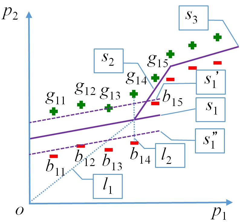
Figure 2: SVM.

Step 2 (Classification by SVMs):

We create a bipartite graph $G$ where good points lie above the bad ones lie in lower and each edge, such as $l_{2}$ in Fig. 2, connects a pair of good and bad points.

Step 2.1: In the $i$-th round, for the points in the set $A_{i}$, a SVM is used to maximize the distance between the nearest training data points, and computes the maximum margin classification between the good and bad points. For the case of 2-dimension, Fig. 2 shows the separation between the good and bad points in $A_{1}$ as follows

• $s_{1}$ is the maximum-margin hyperplane;

• the distance between lines $s_{1}^{\prime}$ and $s_{1}^{\prime\prime}$ is the maximum-margin; and

• the points, such as $g_{1,3}$ and $b_{1,2}$, which lie on line $s_{1}^{\prime}$ or $s_{1}^{\prime\prime}$ are the support vectors.

Thus, we have obtained the maximum-margin hyper-plane $s_{1}$ as the separation boundary (i.e. decision surface), i.e. $s_{1}^{\prime}$ and $s_{1}^{\prime\prime}$ have the maximum-margin. According to the property of SVM, the maximum-margin ensures that the separation that has the highest generalization ability. The learning process of SVM also has a strategy that if there does not exists a single hyperplane to separate all good and bad points in $A_{1}$, the points with smaller indices are separated before the points with larger indices.

Step 2.2: We represent $A_{i}$ as the array $A_{i}=((g_{i1},b_{i1}),\ldots,(g_{in_{i}},b_{in_{i}}))$. If single hyperplane cannot be found in Step 2.1 to separate $G_{i}$ and $B_{i}$ in $A_{i}$, we check through the vector $A_{i}$ from the left to the right to find the first pair, say $(g_{ik},b_{ik})$ that cannot be separated (e.g. $(g_{1,5},b_{1,5})$ in Fig. 2). We call the pairs before $(g_{ik},b_{ik})$ covered (by the checking process) [22], and denote it as $C_{i}$, and the rest pairs of $A_{i}$ are uncovered and denoted as $U_{i}$. For example, $C_{1}=\{g_{11},g_{12},g_{13},g_{14},b_{11},b_{12},b_{13},b_{14}\}$ in Fig 2. We take the hyperplane (e.g. $s_{1}$ in Fig. 2) that separates $C_{i}$ as a boundary segment for separating the good and bad points of $A_{i}$. Then we set the array $A_{i}$ as the $U_{i}$ and go back the SVM process in Step 2.1. If a hyperplane is found to separate these pairs, add the hyperplane to the boundary segments which have found, and repeat the process, otherwise.

Step 3 (Continuous Parameters Generation and Classification): In the same way as the boundary is obtained by previous two steps, we generate a new set of pairs of good and bad points in the new round. Each good or bad point is generated near the boundary generated by the end of Step 2 with the distance of the point to its nearest hyperplane being a given margin $w$ ($w$ can be assigned to be 1 in consideration of the integer-related feature of our problem). The algorithm repeats Step 2 to generate refined boundaries until reaching a given number of iterations or meeting some given criteria for termination.

VI Conclusion

We have studied the parametric synthesis problem for parametric timed automata. We have provided an algorithm to construct the feasible parameter region when PTA with one parametric clock and one parameter. We have proved that, if PTA is restricted to be with only lower-bound or upper-bound parameters, the parametric synthesis problem is solvable. Furthermore, we have shown that the feasible parameter region of more general L/U automata is a “single connected” set for a property which contains existential quantifiers only. Aided by this result, we have presented a SVM based method to compute the boundaries of feasible parameter regions.

In the further, in the theorem phase, we will extend decidable result of parameter synthesis problem in PTA with one parametrically constrained clock and many paramters. In the algorithm phase, we will give the experience result of our algorithm in some test cases.

References

- [1] R. Alur and D. Dill, “Automata for modeling real-time systems,” in Automata, Languages and Programming. Springer Berlin Heidelberg, 1990, pp. 322–335.
- [2] R. Alur and D. L. Dill, “A theory of timed automata,” Theoretical Computer Science, vol. 126, no. 2, pp. 183–235, 1994.
- [3] R. Alur, T. A. Henzinger, and M. Y. Vardi, “Parametric real-time reasoning,” in Proceedings of the twenty-fifth annual ACM symposium on Theory of computing. ACM, 1993, pp. 592–601.
- [4] A. Annichini, E. Asarin, and A. Bouajjani, “Symbolic techniques for parametric reasoning about counter and clock systems,” in Computer Aided Verification. Springer, 2000, pp. 419–434.
- [5] G. Bandini, R. Spelberg, R. C. de Rooij, and W. Toetenel, “Application of parametric model checking-the root contention protocol,” in System Sciences, 2001. Proceedings of the 34th Annual Hawaii International Conference on. IEEE, 2001, pp. 10–pp.
- [6] T. Hune, J. Romijn, M. Stoelinga, and F. Vaandrager, “Linear parametric model checking of timed automata,” The Journal of Logic and Algebraic Programming, vol. 52-53, pp. 183 – 220, 2002.
- [7] L. Bozzelli and S. La Torre, “Decision problems for lower/upper bound parametric timed automata,” Formal Methods in System Design, vol. 35, no. 2, p. 121, 2009.
- [8] R. Alur, K. Etessami, S. La Torre, and D. Peled, “Parametric temporal logic for “model measuring”,” ACM Transactions on Computational Logic (TOCL), vol. 2, no. 3, pp. 388–407, 2001.
- [9] M. Knapik and W. Penczek, “Smt-based parameter synthesis for l/u automata,” in PNSE, 2012, pp. 77–92.
- [10] É. André and D. Lime, “Liveness in l/u-parametric timed automata,” in ACSD, 2017, pp. 9–18.
- [11] A. Jovanović, D. Lime, and O. H. Roux, “Integer parameter synthesis for real-time systems,” IEEE Transactions on Software Engineering, vol. 41, no. 5, pp. 445–461, 2015.
- [12] D. Bundala and J. Ouaknine, “Advances in parametric real-time reasoning,” in International Symposium on Mathematical Foundations of Computer Science. Springer, 2014, pp. 123–134.
- [13] G. Frehse, S. K. Jha, and B. H. Krogh, “A counterexample-guided approach to parameter synthesis for linear hybrid automata,” in Hybrid Systems: Computation and Control. Springer, 2008, pp. 187–200.
- [14] É. André, T. Chatain, L. Fribourg, and E. Encrenaz, “An inverse method for parametric timed automata,” International Journal of Foundations of Computer Science, vol. 20, no. 05, pp. 819–836, 2009.
- [15] É. André and N. Markey, “Language preservation problems in parametric timed automata,” in International Conference on Formal Modeling and Analysis of Timed Systems. Springer, 2015, pp. 27–43.
- [16] M. Knapik and W. Penczek, “Transactions on petri nets and other models of concurrency v,” K. Jensen, S. Donatelli, and J. Kleijn, Eds. Berlin, Heidelberg: Springer-Verlag, 2012, ch. Bounded Model Checking for Parametric Timed Automata, pp. 141–159.
- [17] N. Benes, P. Bezdĕk, K. G. Larsen, and J. Srba, “Language emptiness of continuous-time parametric timed automata,” international colloquium on automata languages and programming, pp. 69–81, 2015.
- [18] J. Li, J. Sun, B. Gao, and A. Étienne, “Classification-based parameter synthesis for parametric timed automata,” in Formal Methods and Software Engineering. Springer International Publishing, 2017, pp. 243–261.
- [19] É. André, “What’s decidable about parametric timed automata?” in Formal Techniques for Safety-Critical Systems. Springer International Publishing, 2016, pp. 52–68.
- [20] R. Alur, “Timed automata,” in Computer Aided Verification. Springer, 1999, pp. 8–22.
- [21] J. Bengtsson and W. Yi, “Timed automata: Semantics, algorithms and tools,” in Lectures on Concurrency and Petri Nets. Springer, 2004, pp. 87–124.
- [22] R. Sharma, A. V. Nori, and A. Aiken, “Interpolants as classifiers,” in Computer Aided Verification. Springer, 2012, pp. 71–87.