LRMM: Learning to Recommend with Missing Modalities

Abstract

Multimodal learning has shown promising performance in content-based recommendation due to the auxiliary user and item information of multiple modalities such as text and images. However, the problem of incomplete and missing modality is rarely explored and most existing methods fail in learning a recommendation model with missing or corrupted modalities. In this paper, we propose LRMM, a novel framework that mitigates not only the problem of missing modalities but also more generally the cold-start problem of recommender systems. We propose modality dropout (m-drop) and a multimodal sequential autoencoder (m-auto) to learn multimodal representations for complementing and imputing missing modalities. Extensive experiments on real-world Amazon data show that LRMM achieves state-of-the-art performance on rating prediction tasks. More importantly, LRMM is more robust to previous methods in alleviating data-sparsity and the cold-start problem.

1 Introduction

Recommender systems (RS) are useful filtering tools which aid customers in a personalized way to make better purchasing decisions and whose recommendations are based on the customer’s preferences and purchasing histories.

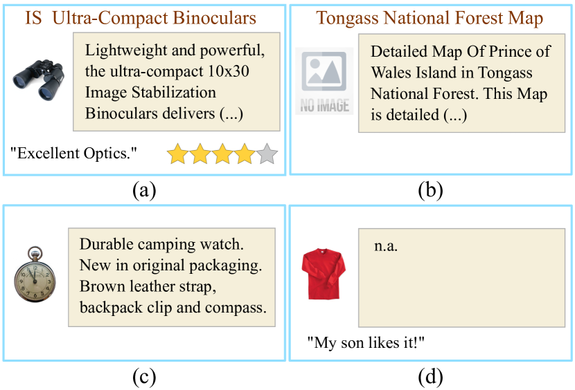
Figure 1: Examples of typical multimodal product data from online retailers: image, title, description, reviews, star ratings. The cold-start problem is present in cases (b) and (c) where neither review text nor ratings are available.

Recommender systems can be roughly divided into collaborative filtering (CF) Koren et al. (2009) or content-based filtering (CBF) Pazzani and Billsus (2007) methods. CF-based methods predict the product preference of users based on their previous purchasing and reviewing behavior by computing latent representations of users and products. Standard matrix factorization (MF) and its variants are widely used in CF approaches Koren et al. (2009). While CF-based approaches were demonstrated to perform well in many application domains Ricci et al. (2015), these methods are based solely on the sparse user-item rating matrix and, therefore, suffer from the so-called cold-start problem Schein et al. (2002); Huang and Lin (2016); Wang et al. (2017) as shown in Figure 1(b)+(c). For new users without a rating history and newly added products with few or no ratings, the systems fail to generate high-quality personalized recommendations.

Alternatively, CBF approaches incorporate auxiliary modalities/information such as product descriptions, images, and user reviews to alleviate the cold-start problem by leveraging the correlations between multiple data modalities. Unfortunately, a pure CBF method often suffers difficulties in generating a recommendation on incomplete and missing data Sedhain et al. (2015); Wang et al. (2016b); Volkovs et al. (2017); García-Durán et al. (2018).

In this work, a multimodal imputation framework (LRMM) is proposed to make RS robust to incomplete and missing modalities. First, LRMM learns multimodal correlations Ngiam et al. (2011); Srivastava and Salakhutdinov (2012); Wang et al. (2016a, 2018) from product images, product metadata (title+description), and product reviews. We propose modality dropout (m-drop) which randomly drops representations of some data modalities. In combination with the modality dropout approach, a sequential autoencoder (m-auto) for multi-modal data is trained to reconstruct missing modalities and, at test time, is used to impute missing modalities through its learned reconstruction function.

Multimodal imputation for recommender systems is a non-trivial issue. (1) Existing RS methods usually assume that all data modalities are available during training and inference. In practice, however, incomplete and missing data modalities are very common. (2) At its core it addresses the cold-start problem. In the context of missing modalities, cold-start can be viewed as missing user or item preference information.

With this paper we make the following contributions:

• For the first time, we introduce multimodal imputation in the context of recommender systems.

• We reformulate the data-sparsity and cold-start problem when data modalities are missing.

• We show that the proposed method achieves state-of-the-art results and is competitive with or outperforms existing methods on multiple data sets.

• We conduct additional extensive experiments to empirically verify that our approach alleviates the missing data modalities problem.

The rest of paper is structured as follows: Section 2 introduces our proposed methods. Section 3 describes the experiments and reports on the empirical results. In section 4 we discuss the method and its advantages and disadvantages, and in section 5 we discuss related work. Section 6 concludes this work.

2 Proposed Methods

The general framework of LRMM is depicted in Figure 2. There are two objectives for LRMM: (1) learning multimodal embeddings that capture inter-modal correlations, complementing missing modalities (Sec. 2.1); (2) learning intra-modal distributions where missing modalities are reconstructed via a missing modality imputation mechanism (sec. 2.2 and 2.3).

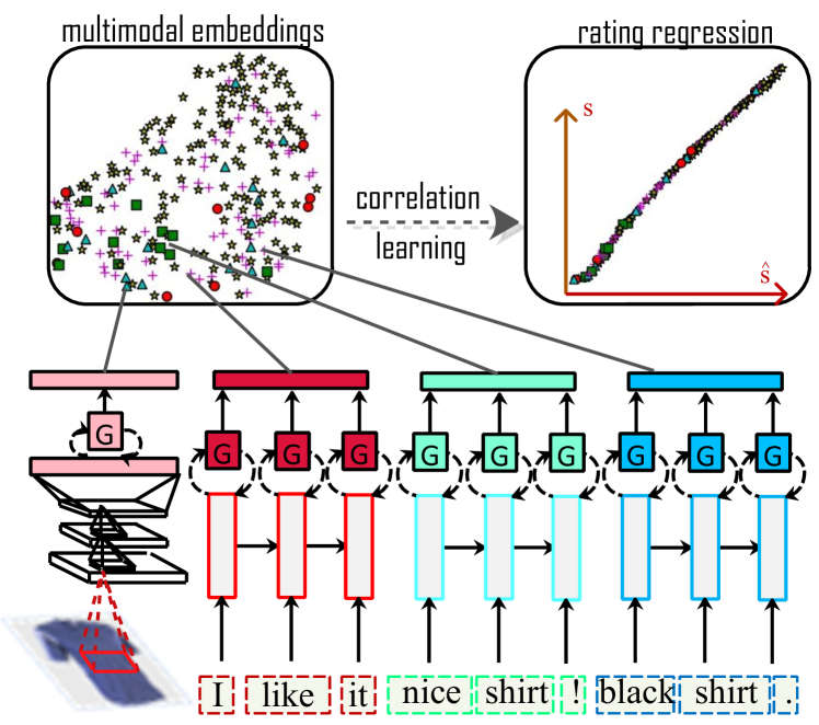
Figure 2: Overview of LRMM. It adopts CNN for visual embeddings (pink part) and three LSTMs for textual embeddings of user review text (red part), item review text (green part) and item meta-data (blue part), respectively. The generative (autoencoder) model is used to reconstruct modality-specific embeddings and impute missing modality. Missing user and item review text lead to user- and item-based cold-start respectively.

2.1 Learning Multimodal Embeddings

We denote a user $\bf{u}$ having $k$ review texts as $\mathbf{r}^{u}$$=$$(r_{o_{1}}^{u},r_{o_{2}}^{u},...,r_{o_{k}}^{u})$ where $r_{o_{i}}^{u}$ represents review text written by $\bf{u}$ for item $o_{i}$. An item $\bf{o}$ is denoted as $\mathbf{r}^{o}$$=$$(r_{u_{1}}^{o},r_{u_{2}}^{o},...,r_{u_{p}}^{o})$ where $r_{u_{j}}^{o}$ represents the review text written by user $\mathbf{u}_{j}$ for item $\bf{o}$. Following Zheng et al. (2017), to represent each user and item, the reviews of $\bf{u}$ and $\bf{o}$ are concatenated into one review history document:

$$\mathbf{D}^{u}=r_{o_{1}}^{u}\oplus r_{o_{2}}^{u}\oplus,...,\oplus r_{o_{k}}^{u}$$ (1)

$$\mathbf{D}^{o}=r_{u_{1}}^{o}\oplus r_{u_{2}}^{o}\oplus,...,\oplus r_{u_{p}}^{o}$$ (2)

where $\oplus$ is the concatenation operator. Similarly, the metadata of each item $\bf{o}$ can be represented as $\mathbf{D}^{m}$. For readability, we use $u,o,m,v$ to denote user, item, metadata, and the image modality, respectively.

For text-based representation learning for user and item, unlike Zheng et al. (2017) in which CNNs (Convolutional Neural Networks) with Word2Vec Mikolov et al. (2013) are employed, our method treats text as sequential data and learns embeddings over word sequences by maximizing the following probabilities:

$$p(\mathbf{x}_{1}^{g},...,\mathbf{x}_{T}^{g})=\prod\nolimits_{t=1}^{T^{g}}p(\mathbf{x}_{t}^{g}|\mathbf{x}_{1}^{g},...,\mathbf{x}_{t-1}^{g})$$ (3)

$$p(\mathbf{x}_{t}^{g}|\mathbf{x}_{1}^{g},...,\mathbf{x}_{t-1}^{g})=p(\mathbf{x}_{t}^{g}|\mathbf{e}_{t}^{g})$$ (4)

$$\mathbf{e}_{t}^{g}=\mathcal{M}^{g}(\mathbf{e}_{t-1}^{g},\mathbf{x}_{t}^{g};\mathbf{\Theta}^{g})$$ (5)

where $\mathcal{M}^{g}$, $g\in\{u,o,m\}$ is a recurrent model and $(\mathbf{x}_{1}^{g},...,\mathbf{x}_{T}^{g})$ is the word sequence of either review or metadata text, each $\mathbf{x}_{t}^{g}\in\mathcal{V}$ and $\mathcal{V}$ is a vocabulary set. $T^{g}$ is the length of input and output sequence and $\mathbf{e}_{t}^{g}$ is the hidden state computed from the corresponding LSTM (Long Short Term Memory) Hochreiter and Schmidhuber (1997) by:

$$\begin{pmatrix}\mathbf{i}_{t}\\ \mathbf{f}_{t}\\ \mathbf{o}_{t}\\ \mathbf{g}_{t}\end{pmatrix}=\begin{pmatrix}\text{sigm}\\ \text{sigm}\\ \text{sigm}\\ \text{tanh}\end{pmatrix}\mathbf{W}\begin{pmatrix}\mathbf{x}_{t}\\ \mathbf{h}_{t-1}\end{pmatrix}$$ (6)

$$\mathbf{c}_{t}=\mathbf{f}_{t}\odot\mathbf{c}_{t-1}+\mathbf{i}_{t}\odot\mathbf{g}_{t}$$ (7)

$$\mathbf{h}_{t}=\mathbf{o}_{t}\odot\tanh(\mathbf{c}_{t})$$ (8)

where $\mathbf{i}_{t}$, $\mathbf{f}_{t}$ and $\mathbf{o}_{t}$ are input, forget and output gate respectively, $\mathbf{c}_{t}$ is memory cell, $\mathbf{h}_{t}$ is the hidden output that we used for computing user or item embedding $\mathbf{e}^{g},~{}g\in\{u,o,m\}$.

As we treat each text document $\mathbf{D}^{g}$ as a word sequence of length $T^{g}$, we adopt average pooling on word embeddings for each modality to obtain document-level representations:

$$\mathbf{e}^{g}=\frac{\sum\nolimits_{t\in T^{g},~{}g\in\{u,o,m\}}\mathbf{e}_{t}^{g}}{T^{g}}$$ (9)

Visual embeddings $\mathbf{e}^{v}$ are extracted with a pre-trained CNN and transformed by a function $f$

$$\mathbf{e}^{v}=f(\mbox{CNN}(I,\mathbf{\Theta}_{c});\mathbf{\Theta}_{f}),$$ (10)

where $\mathbf{\Theta}_{f}\in\mathbb{R}^{4096\times d}$ to ensure $\mathbf{e}^{v}$ has same dimension as the user $\mathbf{e}^{u}$, item $\mathbf{e}^{o}$, and metadata embedding $\mathbf{e}^{m}$. The multimodal joint embedding then can be learned by a shared layer and used for making a prediction:

$$\mathbf{\hat{s}}=f_{s}(\mathbf{W}_{s}(\mathbf{e}^{u}\oplus\mathbf{e}^{o}\oplus\mathbf{e}^{m}\oplus\mathbf{e}^{v})+\mathbf{b}_{s})$$ (11)

where $f_{s}:\mathbb{R}^{4\times d}\rightarrow\mathbb{R}^{1}$, parameterized with $\mathbf{W}_{s}$ and $\mathbf{b}_{s}$, is a scoring function to map the multimodal joint embedding to a rating score.

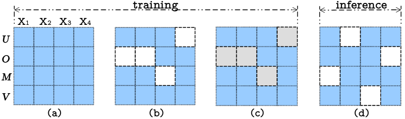
Figure 3: Missing modality imputation. (a) Full training data, (b) m-drop randomly drops modalities, (c) m-auto learns to reconstruct missing data based on existing data. (d) Inference with missing modalities. Dropping user and item view is equivalent to learning models being able to address cold-start problem.

2.2 Modality Dropout

Modality dropout (m-drop) is designed to remove a data modality during training according to some parametric distribution. This is motivated by dropout Srivastava et al. (2014) which randomly masks hidden layer activations to zero to increase the generalization capability of the underlying model. More formally, m-drop changes the original feed-forward equation:

$$\mathbf{Z}^{(L+1)}=\varphi(\mathbf{W}^{(L+1))}\mathbf{X}^{(L)}+\mathbf{b}^{(L+1)})$$ (12)

being able to randomly drop modality by:

$$r^{(L)}\sim\text{Bernoulli}~{}(p_{m})$$ (13)

$$k^{(L)}\sim\text{Bernoulli}~{}(1-1/n_{m})$$ (14)

$$\mathbf{\widetilde{X}}^{(L)}=(\mathbf{X}^{(L)}\odot\mathbf{r}^{(L)})\odot\mathbf{k}^{(L)}$$ (15)

$$\mathbf{Z}^{(L+1)}=\varphi(\mathbf{W}^{(L+1))}\mathbf{\widetilde{X}}^{(L)}+\mathbf{b}^{(L+1)})$$ (16)

where each sample $\mathbf{X}_{1}={x_{1},...,x_{n_{m}}}$ and $n_{m}$ is the number of modalities. $\mathbf{r}^{(L)}$ is a vector of independent Bernoulli random variables each of which has probability $p_{m}$ of being 1. $\mathbf{k}^{(L)}$ is a vector of independent variables which indicate the dropout on modality with a given probability. $\varphi(\cdot)$ is an activation function.

Figure 3 (a-b) shows how m-drop works. Note the differences between modality dropout (m-drop) and original dropout: (1) m-drop targets specifically the multimodal scenario where some modalities are completely missing; and (2) m-drop is performed on the input layer ($L\equiv 0$).

2.3 Mutlimodal Sequential Autoencoder

The autoencoder has been used in prior work Sedhain et al. (2015); Strub et al. (2016) to reconstruct missing elements (mostly ratings) in recommender systems. This is equivalent to the case of missing at random (MAR). For MAR, it is rare to have a continuous large block of missing entries Tran et al. (2017). Differently, in recommending with missing modality, the missing entries typically occur in a large continuous block. For instance, an extreme case is the absence of all item reviews and ratings (data sparsity is 100%, leading to the so-called item cold-start problem). Existing methods Lee and Seung (2000); Koren (2008); Marlin (2003); Wang and Blei (2011); McAuley and Leskovec (2013); Li et al. (2017); Zheng et al. (2017) have difficulties when entire data modalities are missing during the training and/or inference stages.

To address this limitation, we propose a multimodal sequence autoencoder (m-auto) to impute textual sequential embeddings and visual embeddings for the missing modalities. Modality-specific autoencoders are placed between the modality-specific encoders (i.e., CNN and LSTMs) and the shared layer (equation 11). The reconstruction layers, therefore, can capture the inter-modal and intra-modal correlations. More formally, for each data modality $g\in\{u,o,m,v\}$, the modality-specific encoder is given as

$$\mathbf{e}_{hid}^{g}=\text{sigm}(\mathbf{W}_{vh}^{g}\mathbf{e}_{in}^{g}+\mathbf{b}_{vh}^{g})$$ (17)

and the modality-decoder is given as

$$\mathbf{e}_{recon}^{g}=\frac{1}{T^{g}}\sum_{t\in T^{g}}\text{sigm}(\mathbf{W}_{hv}^{g}\mathbf{e}_{hid}^{g}+\mathbf{b}_{hv}^{g})$$ (18)

where $\mathbf{W}_{vh}\in\mathbb{R}^{d\times d_{h}}$ and $\mathbf{W}_{hv}\in\mathbb{R}^{d_{h}\times d}$ are weights, $\mathbf{b}_{vh}$, $\mathbf{b}_{hv}$ are biases receptively for visible-to-hidden, and hidden-to-visible layers. $\mathbf{e}_{in}^{g}$, $\mathbf{e}_{hid}^{g}$ present the original, hidden word-level embeddings, and $\mathbf{e}_{recon}^{g}$ is the reconstructed document-level embeddings. The $\mathbf{e}^{g}$ is a modality-specific embedding.

m-auto is different from previous reconstruction modelsSedhain et al. (2015); Strub et al. (2016) in that its reconstructions are based on inter-modal and intra-modal correlations in the context of multimodal learning.

2.4 Model Optimization

The optimization of the network is formulated as a regression problem by minimizing the mean squared error (MSE) loss $\mathcal{L}_{reg}$:

$$\mathcal{L}_{reg}=\frac{1}{\mathcal{|D|}}\sum_{(u,o,m,v)\in\mathcal{D}}(\mathbf{\hat{s}}-\mathbf{s})^{2}+\lambda\parallel\mathbf{\Theta}_{r}\parallel_{2}$$ (19)

where $\mathbf{\hat{s}}$ and $\mathbf{s}$ are the predicted and truth rating scores. $\mathcal{|D|}$ is dataset size , $\lambda$ is weight decay parameter and $\mathbf{\Theta}_{r}$ is regression model parameters. To constrain the representations to be compact in reconstruction, a penalty term is utilized

$$\mathcal{H}=\sum_{i=1}^{h_{n}}\log\frac{\rho}{\hat{\rho}_{i}}+(1-\rho)\log\frac{1-\rho}{1-\hat{\rho}_{i}}$$ (20)

where $\rho$ and $\hat{\rho}$ are sparsity parameters and average activation of hidden unit $i$, $h_{n}$ is the number of hidden units. The reconstruction loss for each modality is now

$$\begin{split}\mathcal{L}_{recon}^{g}=&\frac{1}{\mathcal{|D|}}\sum_{g\in\{u,o,m,v\}}\left\|\mathbf{e}_{recon}^{g}-\mathbf{e}_{in}^{g}\right\|^{2}\\ &+\lambda_{\rho}\sum_{g\in\{u,o,m,v\}}\mathcal{H}^{g}\end{split}$$ (21)

where $\lambda_{\rho}$ is a sparsity regularization term. The objective of the entire model is then

$$\begin{split}\mathcal{L}=\alpha\mathcal{L}_{reg}+\beta\sum_{g\in\{u,o,m,v\}}\mathcal{L}_{recon}^{g}\end{split}$$ (22)

where $\alpha$ and $\beta$ are learnable parameters. The model is learned in an end-to-end fashion through back-prorogation LeCun et al. (1989).

3 Experiments

This section evaluates LRMM on rating prediction tasks with real-world datasets. We firstly compare LRMM with recent methods (sec. 3.4), then we empirically show the effectiveness of LRMM in alleviating the cold-start, the incomplete/missing data, and the data sparsity problem (sec. 3.5-3.8).

3.1 Datasets and Evaluation Metrics

We conducted experiments on the Amazon dataset McAuley et al. (2015); He and McAuley (2016), which is widely used for the study of recommender systems. It consists of different modalities such as text, image, and numerical data. We used 4 out of 21 categories: Sports and Outdoors (S&O), Health and Personal Care (H&P), Movies and TV, Electronics. Some statistics of the datasets are listed in Table 1. We randomly split each dataset into 80% training, 10% validation, and 10% test data. Each input instance consists of four parts $\mathbf{x}^{(i)}$$=$$(\mathbf{x}^{(i)}_{u},\mathbf{x}^{(i)}_{o},\mathbf{x}^{(i)}_{m},\mathbf{x}^{(i)}_{v})$, where $\mathbf{x}^{(i)}_{u}$ and $\mathbf{x}^{(i)}_{i}$ are the concatenated reviews of users and items in the training data. $\mathcal{V}$ is the vocabulary that was built based on reviews and metadata on the training data. Words with an absolute frequency of at least $20$ are included in the vocabulary.

Table 1: Datasets

Dataset	S&O	H&P	Movie	Electronics
Users	35494	38599	111149	192220
Items	16415	17909	27019	59782
Samples	272453	336769	974582	1614105
$\mathcal{|V|}$	42095	47476	160117	198598

To evaluate the proposed models on the task of rating prediction, we employed two metrics, namely, Root Mean Square Error (RMSE)

$$RMSE=\sqrt{\frac{1}{\mathcal{|D|}}\sum_{(u,o,m,v)\in\mathcal{D}}(\mathbf{\hat{s}}_{i,j}-\mathbf{s}_{i,j})^{2}}$$ (23)

and Mean Absolute Error (MAE)

$$MAE=\frac{1}{\mathcal{|D|}}\sum_{(u,o,m,v)\in\mathcal{D}}\left|\mathbf{\hat{s}}_{i,j}-\mathbf{s}_{i,j}\right|$$ (24)

where $\mathbf{\hat{s}}_{i,j}$ and $\mathbf{s}_{i,j}$ represent the predicted rating score and ground truth rating score that user $i$ gave to item $j$.

Table 2: Comparison on datasets with the baselines. ‘+F’: tested with all modalities(U,O,M,V), ‘-X’: dropping one modality, ‘-U’ and ‘-O’: user and item cold-start scenario.

Dataset	S&O		H&P		Movie		Electronics
Models	RMSE	MAE	RMSE	MAE	RMSE	MAE	RMSE	MAE
Offset	0.979	0.769	1.247	0.882	1.389	0.933	1.401	0.928
NMF	0.948	0.671	1.059	0.761	1.135	0.794	1.297	0.904
SVD++	0.922	0.669	1.026	0.760	1.049	0.745	1.194	0.847
URP	-	-	-	-	1.006	0.764	1.126	0.860
RMR	-	-	-	-	1.005	0.741	1.123	0.822
HFT	0.924	0.659	1.040	0.757	0.997	0.735	1.110	0.807
DeepCoNN	0.943	0.667	1.045	0.746	1.014	0.743	1.109	0.797
NRT	-	-	-	-	0.985	0.702	1.107	0.806
LRMM(+F)	0.886	0.624	0.988	0.708	0.983	0.716	1.052	0.766
LRMM(-U)	0.936	0.719	1.058	0.782	1.086	0.821	1.138	0.900
LRMM(-O)	0.931	0.680	1.039	0.805	1.074	0.855	1.101	0.864
LRMM(-M)	0.887	0.625	0.989	0.710	0.991	0.725	1.053	0.766
LRMM(-V)	0.886	0.624	0.989	0.708	0.991	0.725	1.052	0.766

3.2 Baselines and Competing Methods

We compare our models with several baselines. The baselines can be categorized into three groups.

• Matrix factorization: NMF Lee and Seung (2000) and SVD++ Koren (2008).

• Topic model methods: URP Marlin (2003), CTR Wang and Blei (2011), HFT McAuley and Leskovec (2013) and RMR Ling et al. (2014).

• Deep learning models: NRT Li et al. (2017) and DeepCoNN Zheng et al. (2017), which are current state-of-the-art approaches.

We also include a naive method—Offset McAuley and Leskovec (2013) which simply takes the average across all training ratings.

3.3 Implementation

We implemented LRMM with Theano. The weights for the non-recurrent layer were initialized by drawing from the interval $\left[-\sqrt{\frac{6}{N_{in}+N_{out}}},\sqrt{\frac{6}{N_{in}+N_{out}}}\right]$ ($N$ is the number of units) uniformly at random. We used 1024 hidden units for the autoencoder. The LSTMs have 256 hidden units and the internal weights $\mathbf{W}$ are orthogonally initialized Saxe et al. (2014). We used a batch size of 256, $\lambda=0.0001$, sparsity parameter $\rho=0.05$, $\lambda_{\rho}=0.01$, an initial learning rate of 0.0001 and a dropout rate of 0.5 after the recurrent layer. The models were optimized with ADADELTA Zeiler (2012). The length of the user, item and meta-data document $\mathbf{D}^{u}$, $\mathbf{D}^{o}$, and $\mathbf{D}^{m}_{o}$ were fixed to $L=100$. We truncated documents with more than 100 words. The image features are extracted from the first fully-connected layer of CNN on ImageNet Russakovsky et al. (2015).

We implemented NMF and SVD++ with the SurPrise package. Offset and HFT were implemented by modifying authors’ implementation. For DeepCoNN, we adapted the implementation from Chen et al. (2018). The numbers of other methods are taken from Li et al. (2017).

3.4 Compare with State-of-the-art

First, we compare LRMM with state-of-the-art methods listed in Sec. 3.2. In this setting, LRMM is trained with all data modalities and tested with different missing modality regimes. Table 2 lists the results on the four datasets. By leveraging multimodal correlations, LRMM significantly outperforms MF-based models (i.e. NMF, SVD++) and topic-based methods (i.e., URP, CTR, RMR, and HFT). LRMM also outperforms recent deep learning models (i.e., NRT, DeepCoNN) with respect to almost all metrics.

LRMM is the only method with a robust performance for the cold-start recommendation problem where user review or item review texts are removed. While the cold-start recommendation is more challenging, LRMM(-U) and LRMM(-O) are still able to achieve a similar performance to the baselines in the standard recommendation setting. For example, RMSE 1.101 (LRMM(-O)) to 1.107 (NRT) on Electronics, MAE 0.680 (LRMM(-O)) to 0.667 (DeepCoNN)on S&O. We conjecture that the cross-modality dependencies Srivastava and Salakhutdinov (2012) make LRMM more robust when modalities are missing. Table 5 lists some randomly selected rating predictions. Similar to Table 2, missing user (-U) and item (-O) preference significantly deteriorates the performance.

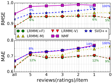
Figure 4: Performance with reduced reviews (ratings) on S&O dataset. (% : performance drops for SVD++ (in blue) and LRMM(+F) (in green))

3.5 Cold-Start Recommendation

Prior work McAuley and Leskovec (2013); Zhang et al. (2017) has considered users (items) with sparse preference information as the cold-start problem (e.g., Figure 1(d)), that is, where there is still some information available. In practice, preference information could be missing in larger quantities or even be entirely absent (e.g., Figure 1(b-c)). In this situation, the aforementioned methods are not applicable as they require some data to work with. In this experiment, we examine how LRMM leverages modality correlations to alleviate the data sparsity problem when training data becomes even sparser. To this end, we train models for the item cold-start problem by reducing the number of reviews (for LRMM) and ratings (for NMF and SVD++) of each item in the training set.

Figure 4 demonstrates the robustness of LRMM when the training data becomes more sparse. Note that NMF and SVD++ fail to train models when there is no ratings data available. In contrast, LRMM is trained by leveraging item images and metadata even if item reviews are completely missing for a product. The average number of reviews per item on this dataset is 16.7. Reducing the number of ratings to 5 severely degrades the performance of NMF, SVD++, and LRMM. However, LRMM remains rather stable in maintaining good performance when considering the performance degradation at 5, 1, and 0 reviews (ratings), respectively. One interesting observation is that, with a reduced number of reviews, the product metadata plays a more and more important role in maintaining the performance: LRMM(-V) is close to LRMM(+F) in Figure 4 while the gap between LRMM(-M) and LRMM(+F) is large.

3.6 Missing Modality Imputation

Table 3: The performance of training with missing modality imputation.

Dataset	S&O		H&P
Models	RMSE	MAE	RMSE	MAE
LRMM(+F)	0.997	0.790	1.131	0.912
LRMM(-U)	0.998	0.795	1.132	0.914
LRMM(-O)	0.999	0.796	1.133	0.917
LRMM(-M)	0.998	0.797	1.133	0.913
LRMM(-V)	0.997	0.791	1.132	0.913

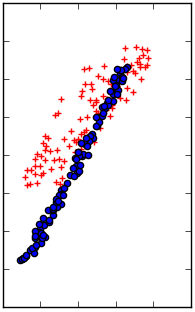
(a) $\mathbf{e}^{v}$

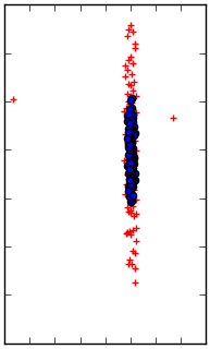
(b) $\mathbf{e}^{u}$

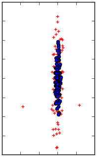
(c) $\mathbf{e}^{o}$

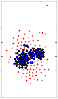
(d) $\mathbf{e}^{m}$

Figure 5: Visualization of embeddings (blue) and reconstructed embeddings (red)

The proposed m-drop and m-auto methods allow LRMM to be more robust to missing data modalities. Table 3 lists the results of training LRMM with missing data modalities for the modality dropout ratio $p_{m}=0.5$ on the S&O and H&P datasets, respectively. Both RMSE and MAE of LRMM deteriorate but are still comparable to the MF-based approaches NMF and SVD++. However, the proposed method LRMM is robust to missing data in both training and inference stages, a problem rarely addressed by existing approaches. In Figure 5, we visualized the modality-specific embeddings and their reconstructed embeddings of 100 randomly selected samples with t-SNE van der Maaten and Hinton (2008). The plots suggest that it is more challenging to reconstruct item metadata and image embeddings as compared to the user or item embeddings. One possible explanation is that some selected metadata contains noisy data (e.g., “ISBN - 9780963235985”, “size: 24 $\times$46” and “Dimensions: 15W $\times$ 22H”) for which visual data is more diverse. This would increase the difficulty of incorporating visual data into the embeddings.

3.7 The Effect of Text Length

To alleviate the data sparsity problem, existing work McAuley and Leskovec (2013); Zhang et al. (2017) concatenates review texts and utilizes topic modeling (e.g. HFT) or CNNs combined with Word2Vec (e.g. DeepCoNN) to learn user or item embeddings. Differently, LRMM treats the concatenated reviews as sequential data and learns sequence embeddings with RNNs. In this experiment, we show that learning sequential embedding is beneficial on sparse data because it is unnecessary to exploit all reviews so as to reach good performance. Figure 6 shows the performance of LRMM with varied word sequence lengths. In general, sequence embeddings learned with larger length achieve better performance. Note that, by considering a certain amount of words (e.g. L=50), LRMM is able to achieve a result as good as accounting more words (e.g. L=100 or 200). Although this is dataset-dependent to some degree, e.g., LRMM (L=200) improves RMSE and MAE in a certain margin as compared to L=100 on the H&P data, it demonstrates the superiority of sequential user or item embeddings as compared to topic and CNN+Word2Vec embeddings on more sparse data as shown in Table 2.

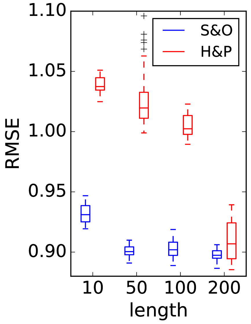
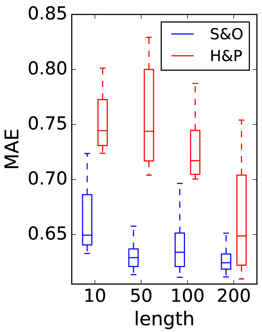
Figure 6: RMSE and MAE with varied text lengths on S&O and H&P datasets.

3.8 Cross-Domain Adaptation

To consider an even more challenging situation we explore cases where the full training set is missing. Inspired by the recent success of domain adaptation (DA) Csurka (2017), a special form of transfer learning Pan and Yang (2010); Weiss et al. (2016), we perform the recommendation task on the target domain test set $\mathcal{D}^{t}_{test}$ (e.g., “Sport”) but with the model $\mathcal{C}$ trained on a different domain training set $\mathcal{D}^{s}_{train}$ (e.g. “Movie”). This is achieved by extracting the multimodal embeddings on the source domain and by performing prediction on the target domain. Table 4 shows the performance of LRMM when performing adaptation from larger datasets to smaller datasets. Although the performance is not as good as on $\mathcal{D}^{s}_{test}$, LRMM is still able to obtain decent results even without using training data $\mathcal{D}^{t}_{train}$. Table 6 shows some example rating predictions on DA for different categories of products. It demonstrates the strong generalization capability of DA from one product category to another.

Table 4: Cross-Domain Adaptation with LRMM

$\mathcal{D}^{s}\rightarrow\mathcal{D}^{t}$	+F	-U	-O	-M	-V
Movie$\rightarrow$S&O	1.061	1.013	1.071	1.061	1.062
Movie$\rightarrow$H&P	1.190	1.140	1.170	1.190	1.190
Elect.$\rightarrow$S&O	1.072	1.012	1.088	1.073	1.073
Elect.$\rightarrow$H&P	1.191	1.137	1.180	1.191	1.192

Table 5: Exemplary rating prediction on S&O datatset. ‘T’ means true ratings, the best prediction is in blue, the worst prediction is in red.

Item image	T	+F	-U	-O	-M	-V
	3	3.18	3.97	3.48	3.03	3.28
	3	3.36	4.07	3.5	3.33	3.27
	5	4.63	4.50	4.36	4.60	4.63
	3	3.11	3.77	3.49	3.44	3.57
	4	4.00	4.31	3.87	3.92	4.02

Table 6: Examples on H&P datatset with domain adaptation. The model is trained on Movie dataset.

Item image	T	+F	-U	-O	-M	-V
	4	4.01	4.18	3.70	4.04	4.05
	2	2.58	3.85	2.82	2.82	2.76
	3	2.97	4.33	2.77	2.99	2.96
	4	4.09	3.68	4.14	4.09	4.04
	5	4.99	4.39	4.47	4.94	5.01

4 Discussion

Empirically, we have shown that multimodal learning (+F) plays an important role in mitigating the problems associated with missing data/modality and, in particular, those associated with the cold-start problem (-U and -O) of recommender systems. The proposed method LRMM is in line and grounded in recent developments (e.g. DeepCoNN, NRT) to incorporate multimodal data. LRMM distinguishes itself from previous methods: (1) the cold-start problem is reformulated in the context of missing modality; (2) A novel multimodal imputation method which consists of m-drop and m-auto is proposed to learn models more robust to missing data modalities in both the training and inference stages.

5 Related Work

Collaborative filtering (CF) is the most commonly used approach for recommender systems. CF methods generally utilize the item-user feedback matrix. Matrix factorization (MF) is the most popular CF method Koren et al. (2009) due to its simplicity, performance, and high accuracy as demonstrated in previous work Chen et al. (2015). Another strength of MF, making it widely used in recommender systems, is that side information other than existing ratings can easily be integrated into the model to further increase its accuracy. Such information includes social network data Li et al. (2015); Lagun and Agichtein (2015); Zhao et al. (2016); Xiao et al. (2017), locations of users and items Lu et al. (2017) and visual appearance He and McAuley (2016); Salakhutdinov and Mnih (2007) proposed Probabilistic Matrix Factorization (PMF) which extends MF to a probabilistic linear model with Gaussian noise. Following PMF, there are many extensions Salakhutdinov et al. (2007); Chen et al. (2013); Zheng et al. (2016); Zhang et al. (2016); He et al. (2016b, 2017) aiming to improve its accuracy.

Unfortunately, CF methods suffer from the cold-start problem when dealing with new items or users without rich information. Content based filtering (CBF) Pazzani and Billsus (2007), on the other hand, is able to alleviate the cold-start problem by taking auxiliary product and user information (texts, images, videos, etc.) into consideration. Recently, several approaches Almahairi et al. (2015); Xu et al. (2014); He et al. (2014); Tan et al. (2016) were proposed to consider the information of review text to address the data sparsity problem which leads to the cold-start problem. The topic model (e.g. LDA Blei et al. (2003)) based approaches including CTR Wang and Blei (2011), HFT McAuley and Leskovec (2013), RMR Ling et al. (2014), TriRank He et al. (2015), and sCVR Ren et al. (2017) achieve significant improvements compared to previous work on recommender systems.

Inspired by the recent success of deep learning techniques Krizhevsky et al. (2012); He et al. (2016a), some deep network based recommendation approaches have been introduced Wang et al. (2015); Sedhain et al. (2015); Wang et al. (2016b); Seo et al. (2017); Xue et al. (2017); Zhang et al. (2017). Deep cooperative neural network (Deep-CoNN) Zheng et al. (2017) was introduced to learn a joint representation from items and users using two coupled network for rating prediction. It is the first approach to represent users and items in a joint manner with review text. TransNets Catherine and Cohen (2017) extends Deep-CoNN by introducing an additional latent layer representing the user-item pair. NRT Li et al. (2017) is a method for rating prediction and abstractive tips generation Zhou et al. (2017). A four-layer neural network was used for rating regression model. NRT outperforms the state-of-the-art methods on rating prediction. There is a large body of work for recommender systems and we refer the reader to for surveys of state-of-the-art CF based approaches, CBF methods, and deep learning based methods, respectively Shi et al. (2014); Lops et al. (2011); Zhang et al. (2017).

Our work differs from previous work in that we simultaneously address various types of missing data together with the data-sparsity and cold-start problems.

6 Conclusion

We presented LRMM, a framework that improves the performance and robustness of recommender systems under missing data. LRMM makes novel contributions in two ways: multimodal imputation and jointly alleviating the missing modality, data sparsity, and cold-start problem for recommender systems. It learns to recommend when entire modalities are missing by leveraging inter- and intra-modal correlations from data through the proposed m-drop and m-auto methods. LRMM achieves state-of-the-art performance on multiple data sets. Empirically, we analyzed LRMM in different data sparsity regimes and demonstrated the effectiveness of LRMM. We aim to explore a generalized domain adaptation approach for recommender systems with missing data modalities.

References

- Almahairi et al. (2015) Amjad Almahairi, Kyle Kastner, Kyunghyun Cho, and Aaron C. Courville. 2015. Learning distributed representations from reviews for collaborative filtering. In RecSys, pages 147–154.
- Blei et al. (2003) David M. Blei, Andrew Y. Ng, and Michael I. Jordan. 2003. Latent dirichlet allocation. Journal of Machine Learning Research, 3:993–1022.
- Catherine and Cohen (2017) Rose Catherine and William W. Cohen. 2017. Transnets: Learning to transform for recommendation. In RecSys, pages 288–296.
- Chai and Draxler (2014) Tianfeng Chai and Roland R Draxler. 2014. Root mean square error (rmse) or mean absolute error (mae)?–arguments against avoiding rmse in the literature. Geoscientific Model Development, 7(3):1247–1250.
- Chen et al. (2018) Chong Chen, Min Zhang, Yiqun Liu, and Shaoping Ma. 2018. Neural attentional rating regression with review-level explanations. In WWW.
- Chen et al. (2013) Tianqi Chen, Hang Li, Qiang Yang, and Yong Yu. 2013. General functional matrix factorization using gradient boosting. In ICML (1), volume 28, pages 436–444.
- Chen et al. (2015) Yun-Nung Chen, William Yang Wang, Anatole Gershman, and Alexander Rudnicky. 2015. Matrix factorization with knowledge graph propagation for unsupervised spoken language understanding. In ACL-IJCNLP, volume 1, pages 483–494.
- Csurka (2017) Gabriela Csurka. 2017. Domain adaptation for visual applications: A comprehensive survey. CoRR, abs/1702.05374.
- García-Durán et al. (2018) Alberto García-Durán, Roberto Gonzalez, Daniel Oñoro-Rubio, Mathias Niepert, and Hui Li. 2018. Transrev: Modeling reviews as translations from users to items. CoRR, abs/1801.10095.
- He et al. (2016a) Kaiming He, Xiangyu Zhang, Shaoqing Ren, and Jian Sun. 2016a. Deep residual learning for image recognition. In CVPR, pages 770–778.
- He and McAuley (2016) Ruining He and Julian McAuley. 2016. Ups and downs: Modeling the visual evolution of fashion trends with one-class collaborative filtering. In WWW, pages 507–517.
- He et al. (2015) Xiangnan He, Tao Chen, Min-Yen Kan, and Xiao Chen. 2015. Trirank: Review-aware explainable recommendation by modeling aspects. In CIKM, pages 1661–1670.
- He et al. (2014) Xiangnan He, Ming Gao, Min-Yen Kan, Yiqun Liu, and Kazunari Sugiyama. 2014. Predicting the popularity of web 2.0 items based on user comments. In SIGIR, pages 233–242.
- He et al. (2017) Xiangnan He, Lizi Liao, Hanwang Zhang, Liqiang Nie, Xia Hu, and Tat-Seng Chua. 2017. Neural collaborative filtering. In WWW, pages 173–182.
- He et al. (2016b) Xiangnan He, Hanwang Zhang, Min-Yen Kan, and Tat-Seng Chua. 2016b. Fast matrix factorization for online recommendation with implicit feedback. In SIGIR, pages 549–558.
- Hochreiter and Schmidhuber (1997) Sepp Hochreiter and Jürgen Schmidhuber. 1997. Long short-term memory. Neural Computation, 9(8):1735–1780.
- Huang and Lin (2016) Yu-Yang Huang and Shou-De Lin. 2016. Transferring user interests across websites with unstructured text for cold-start recommendation. In EMNLP, pages 805–814.
- Koren (2008) Yehuda Koren. 2008. Factorization meets the neighborhood: a multifaceted collaborative filtering model. In KDD, pages 426–434.
- Koren et al. (2009) Yehuda Koren, Robert M. Bell, and Chris Volinsky. 2009. Matrix factorization techniques for recommender systems. IEEE Computer, 42(8):30–37.
- Krizhevsky et al. (2012) Alex Krizhevsky, Ilya Sutskever, and Geoffrey E. Hinton. 2012. Imagenet classification with deep convolutional neural networks. In NIPS, pages 1106–1114.
- Lagun and Agichtein (2015) Dmitry Lagun and Eugene Agichtein. 2015. Inferring searcher attention by jointly modeling user interactions and content salience. In SIGIR, pages 483–492.
- LeCun et al. (1989) Yann LeCun, Bernhard E. Boser, John S. Denker, Donnie Henderson, Richard E. Howard, Wayne E. Hubbard, and Lawrence D. Jackel. 1989. Backpropagation applied to handwritten zip code recognition. Neural Computation, 1(4):541–551.
- Lee and Seung (2000) Daniel D. Lee and H. Sebastian Seung. 2000. Algorithms for non-negative matrix factorization. In NIPS, pages 556–562.
- Li et al. (2015) Hui Li, Dingming Wu, Wenbin Tang, and Nikos Mamoulis. 2015. Overlapping community regularization for rating prediction in social recommender systems. In RecSys, pages 27–34.
- Li et al. (2017) Piji Li, Zihao Wang, Zhaochun Ren, Lidong Bing, and Wai Lam. 2017. Neural rating regression with abstractive tips generation for recommendation. In SIGIR, pages 345–354.
- Ling et al. (2014) Guang Ling, Michael R. Lyu, and Irwin King. 2014. Ratings meet reviews, a combined approach to recommend. In RecSys, pages 105–112.
- Lops et al. (2011) Pasquale Lops, Marco de Gemmis, and Giovanni Semeraro. 2011. Content-based recommender systems: State of the art and trends. In Recommender Systems Handbook, pages 73–105. Springer.
- Lu et al. (2017) Ziyu Lu, Hui Li, Nikos Mamoulis, and David W. Cheung. 2017. HBGG: a hierarchical bayesian geographical model for group recommendation. In SDM, pages 372–380.
- van der Maaten and Hinton (2008) Laurens van der Maaten and Geoffrey Hinton. 2008. Visualizing data using t-sne. Journal of Machine Learning Research, 9:2579–2605.
- Marlin (2003) Benjamin M. Marlin. 2003. Modeling user rating profiles for collaborative filtering. In NIPS, pages 627–634.
- McAuley and Leskovec (2013) Julian J. McAuley and Jure Leskovec. 2013. Hidden factors and hidden topics: understanding rating dimensions with review text. In RecSys, pages 165–172.
- McAuley et al. (2015) Julian J. McAuley, Christopher Targett, Qinfeng Shi, and Anton van den Hengel. 2015. Image-based recommendations on styles and substitutes. In SIGIR, pages 43–52.
- Mikolov et al. (2013) Tomas Mikolov, Ilya Sutskever, Kai Chen, Gregory S. Corrado, and Jeffrey Dean. 2013. Distributed representations of words and phrases and their compositionality. In NIPS, pages 3111–3119.
- Ngiam et al. (2011) Jiquan Ngiam, Aditya Khosla, Mingyu Kim, Juhan Nam, Honglak Lee, and Andrew Y. Ng. 2011. Multimodal deep learning. In ICML, pages 689–696.
- Pan and Yang (2010) Sinno Jialin Pan and Qiang Yang. 2010. A survey on transfer learning. IEEE Trans. Knowl. Data Eng., 22(10):1345–1359.
- Pazzani and Billsus (2007) Michael J. Pazzani and Daniel Billsus. 2007. Content-based recommendation systems. In The Adaptive Web, volume 4321 of Lecture Notes in Computer Science, pages 325–341.
- Ren et al. (2017) Zhaochun Ren, Shangsong Liang, Piji Li, Shuaiqiang Wang, and Maarten de Rijke. 2017. Social collaborative viewpoint regression with explainable recommendations. In WSDM, pages 485–494.
- Ricci et al. (2015) Francesco Ricci, Lior Rokach, and Bracha Shapira, editors. 2015. Recommender Systems Handbook. Springer.
- Russakovsky et al. (2015) Olga Russakovsky, Jia Deng, Hao Su, Jonathan Krause, Sanjeev Satheesh, Sean Ma, Zhiheng Huang, Andrej Karpathy, Aditya Khosla, Michael S. Bernstein, Alexander C. Berg, and Fei-Fei Li. 2015. Imagenet large scale visual recognition challenge. International Journal of Computer Vision, 115(3):211–252.
- Salakhutdinov and Mnih (2007) Ruslan Salakhutdinov and Andriy Mnih. 2007. Probabilistic matrix factorization. In NIPS, pages 1257–1264.
- Salakhutdinov et al. (2007) Ruslan Salakhutdinov, Andriy Mnih, and Geoffrey E. Hinton. 2007. Restricted boltzmann machines for collaborative filtering. In ICML, volume 227, pages 791–798.
- Saxe et al. (2014) Andrew M. Saxe, James L. McClelland, and Surya Ganguli. 2014. Exact solutions to the nonlinear dynamics of learning in deep linear neural networks. In ICLR.
- Schein et al. (2002) Andrew I. Schein, Alexandrin Popescul, Lyle H. Ungar, and David M. Pennock. 2002. Methods and metrics for cold-start recommendations. In SIGIR, pages 253–260.
- Sedhain et al. (2015) Suvash Sedhain, Aditya Krishna Menon, Scott Sanner, and Lexing Xie. 2015. Autorec: Autoencoders meet collaborative filtering. In WWW (Companion Volume), pages 111–112.
- Seo et al. (2017) Sungyong Seo, Jing Huang, Hao Yang, and Yan Liu. 2017. Interpretable convolutional neural networks with dual local and global attention for review rating prediction. In RecSys, pages 297–305.
- Shi et al. (2014) Yue Shi, Martha Larson, and Alan Hanjalic. 2014. Collaborative filtering beyond the user-item matrix: A survey of the state of the art and future challenges. ACM Comput. Surv., 47(1):3:1–3:45.
- Srivastava et al. (2014) Nitish Srivastava, Geoffrey E. Hinton, Alex Krizhevsky, Ilya Sutskever, and Ruslan Salakhutdinov. 2014. Dropout: a simple way to prevent neural networks from overfitting. Journal of Machine Learning Research, 15(1):1929–1958.
- Srivastava and Salakhutdinov (2012) Nitish Srivastava and Ruslan Salakhutdinov. 2012. Multimodal learning with deep boltzmann machines. In NIPS, pages 2231–2239.
- Strub et al. (2016) Florian Strub, Romaric Gaudel, and Jérémie Mary. 2016. Hybrid recommender system based on autoencoders. In Proceedings of the 1st Workshop on Deep Learning for Recommender Systems, pages 11–16. ACM.
- Tan et al. (2016) Yunzhi Tan, Min Zhang, Yiqun Liu, and Shaoping Ma. 2016. Rating-boosted latent topics: Understanding users and items with ratings and reviews. In IJCAI, pages 2640–2646.
- Tran et al. (2017) Luan Tran, Xiaoming Liu, Jiayu Zhou, and Rong Jin. 2017. Missing modalities imputation via cascaded residual autoencoder. In Proceedings of the IEEE Conference on Computer Vision and Pattern Recognition, pages 1405–1414.
- Volkovs et al. (2017) Maksims Volkovs, Guang Wei Yu, and Tomi Poutanen. 2017. Dropoutnet: Addressing cold start in recommender systems. In NIPS, pages 4964–4973.
- Wang et al. (2016a) Cheng Wang, Haojin Yang, and Christoph Meinel. 2016a. A deep semantic framework for multimodal representation learning. Multimedia Tools Appl., 75(15):9255–9276.
- Wang et al. (2018) Cheng Wang, Haojin Yang, and Christoph Meinel. 2018. Image captioning with deep bidirectional lstms and multi-task learning. ACM Transactions on Multimedia Computing, Communications, and Applications (TOMM), 14(2s):40.
- Wang and Blei (2011) Chong Wang and David M. Blei. 2011. Collaborative topic modeling for recommending scientific articles. In KDD, pages 448–456.
- Wang et al. (2016b) Hao Wang, Xingjian Shi, and Dit-Yan Yeung. 2016b. Collaborative recurrent autoencoder: Recommend while learning to fill in the blanks. In NIPS, pages 415–423.
- Wang et al. (2015) Hao Wang, Naiyan Wang, and Dit-Yan Yeung. 2015. Collaborative deep learning for recommender systems. In KDD, pages 1235–1244.
- Wang et al. (2017) Xuepeng Wang, Kang Liu, and Jun Zhao. 2017. Handling cold-start problem in review spam detection by jointly embedding texts and behaviors. In ACL, volume 1, pages 366–376.
- Weiss et al. (2016) Karl R. Weiss, Taghi M. Khoshgoftaar, and Dingding Wang. 2016. A survey of transfer learning. J. Big Data, 3:9.
- Xiao et al. (2017) Lin Xiao, Zhang Min, Yongfeng Zhang, Yiqun Liu, and Shaoping Ma. 2017. Learning and transferring social and item visibilities for personalized recommendation. In CIKM, pages 337–346.
- Xu et al. (2014) Yinqing Xu, Wai Lam, and Tianyi Lin. 2014. Collaborative filtering incorporating review text and co-clusters of hidden user communities and item groups. In CIKM, pages 251–260.
- Xue et al. (2017) Hong-Jian Xue, Xinyu Dai, Jianbing Zhang, Shujian Huang, and Jiajun Chen. 2017. Deep matrix factorization models for recommender systems. In IJCAI, pages 3203–3209.
- Zeiler (2012) Matthew D Zeiler. 2012. Adadelta: an adaptive learning rate method. arXiv preprint arXiv:1212.5701.
- Zhang et al. (2016) Hanwang Zhang, Fumin Shen, Wei Liu, Xiangnan He, Huanbo Luan, and Tat-Seng Chua. 2016. Discrete collaborative filtering. In SIGIR, pages 325–334.
- Zhang et al. (2017) Shuai Zhang, Lina Yao, and Aixin Sun. 2017. Deep learning based recommender system: A survey and new perspectives. CoRR, abs/1707.07435.
- Zhao et al. (2016) Wayne Xin Zhao, Sui Li, Yulan He, Edward Y. Chang, Ji-Rong Wen, and Xiaoming Li. 2016. Connecting social media to e-commerce: Cold-start product recommendation using microblogging information. IEEE Trans. Knowl. Data Eng., 28(5):1147–1159.
- Zheng et al. (2017) Lei Zheng, Vahid Noroozi, and Philip S. Yu. 2017. Joint deep modeling of users and items using reviews for recommendation. In WSDM, pages 425–434.
- Zheng et al. (2016) Yin Zheng, Bangsheng Tang, Wenkui Ding, and Hanning Zhou. 2016. A neural autoregressive approach to collaborative filtering. In ICML, volume 48, pages 764–773.
- Zhou et al. (2017) Ming Zhou, Mirella Lapata, Furu Wei, Li Dong, Shaohan Huang, and Ke Xu. 2017. Learning to generate product reviews from attributes. In EACL (1), pages 623–632.