A year in the life of GW170817: the rise and fall of a structured jet from a binary neutron star merger

Abstract

We present the results of our year-long afterglow monitoring of GW170817, the first binary neutron star (NS) merger detected by advanced LIGO and advanced Virgo. New observations with the Australian Telescope Compact Array (ATCA) and the Chandra X-ray Telescope were used to constrain its late-time behavior. The broadband emission, from radio to X-rays, is well-described by a simple power-law spectrum with index $\beta$ $\sim$0.585 at all epochs. After an initial shallow rise $\propto$ $t^{0.9}$, the afterglow displayed a smooth turn-over, reaching a peak X-ray luminosity of $L_{X}$$\approx$5$\times$$10^{39}$ erg s^-1 at 160 d, and has now entered a phase of rapid decline, approximately $\propto$ $t^{-2}$. The latest temporal trend challenges most models of choked jet/cocoon systems, and is instead consistent with the emergence of a relativistic structured jet seen at an angle of $\approx$22^∘ from its axis. Within such model, the properties of the explosion (such as its blastwave energy $E_{K}\approx 2\times 10^{50}$ erg, jet width $\theta_{c}$ $\approx$4^∘, and ambient density $n$ $\approx$3$\times$ $10^{-3}$ cm^-3) fit well within the range of properties of cosmological short GRBs.

1 Introduction

On August 17^th, 2017 the Advanced LIGO interferometers detected the first gravitational wave (GW) signal from a binary neutron star (NS) merger, GW170817, followed 1.7 s later by a short duration gamma-ray burst, GRB170817A (Abbott et al., 2017a). Located in the elliptical galaxy NGC4993 at a distance of $\sim$40 Mpc, GRB170817A was an atypical sub-luminous explosion. An X-ray afterglow was detected 9 days after the merger (Troja et al., 2017). A second set of observations, performed $\sim$15 days post-merger, revealed that the emission was not fading, as standard GRB afterglows, but was instead rising at a slow rate (Troja et al., 2017; Haggard et al., 2017). The radio afterglow, detected at 16 days (Hallinan et al., 2017), continued to rise in brightness (Mooley et al., 2018a), as later confirmed by X-ray and optical observations (Troja et al., 2018a; D’Avanzo et al., 2018; Lyman et al., 2018; Margutti et al., 2018).

The delayed afterglow onset and low-luminosity of the $\gamma$-ray signal could be explained if the jet was observed at an angle (off-axis) of $\approx$15^∘-30^∘. Whereas a standard uniform jet viewed off-axis could account for the early afterglow emission, Troja et al. (2017) and Kasliwal et al. (2017) noted that it could not account for the observed gamma-ray signal and proposed two alternative models: a structured jet, i.e. a jet with an angular profile of Lorentz factors and energy (see also Abbott et al., 2017a; Kathirgamaraju et al., 2018), and a mildly-relativistic isotropic cocoon (see also Lazzati et al., 2017; Kasliwal et al., 2017). In the latter model, the jet may never emerge from the merger ejecta (choked jet).

The subsequent rebrightening ruled out both the uniform jet and the simple cocoon models, which predict a sharp afterglow rise. It was instead consistent with an off-axis structured jet (Troja et al., 2017) and a cocoon with energy injection (Mooley et al., 2018a), characterized by a radial profile of ejecta velocities. In Troja et al. (2018a) we developed semi-analytical models for both the structured jet and the quasi-spherical cocoon with energy injection, and showed that they describe the broadband afterglow evolution during the first six months (from the afterglow onset to its peak) equally well. This is confirmed by numerical simulations of relativistic jets (Lazzati et al., 2018; Xie et al., 2018) and choked jets (Nakar, et al., 2018).

Several tests were discussed to distinguish between these two competing models (e.g. Gill & Granot, 2018; Nakar, et al., 2018). Corsi et al. (2018) used the afterglow polarization to probe the outflow geometry (collimated vs. nearly isotropic), but the results were not constraining. Ghirlanda, et al. (2019) and Mooley et al. (2018b) used Very Long Baseline Interferometry (VLBI) to image the radio counterpart, and concluded that the compact source size ($\lesssim$2 mas) and its apparent superluminal motion favor the emergence of a relativistic jet core. A third and independent way to probe the outflow structure is to follow its late-time temporal evolution. In the case of a cocoon-dominated emission, the afterglow had been predicted to follow a shallow decay ($t^{-\alpha}$) with $\alpha$ $\sim$1.0-1.2 (Troja et al., 2018a) for a quasi-spherical outflow, and $\alpha$ $\sim$1.35 for a wide-angled cocoon (Lamb, Mandel & Resmi, 2018). A relativistic jet is instead expected to resemble a standard on-axis explosion at late-times, thus displaying a post-jet-break decay of $\alpha\sim 2.5$ (van Eerten & MacFadyen, 2013).

Here, we present the results of our year-long observing campaign of GW170817, carried out with the Australian Telescope Compact Array (ATCA) in the radio, Hubble Space Telescope (HST) in the optical, the Chandra X-ray telescope and XMM-Newton in the X-rays. Our latest observations show no signs of spectral evolution (Sect. 2.1) and a rapid decline of the afterglow emission (Sect. 2.2), systematically faster than cocoon-dominated/choked jet models from the literature (Sect. 3.1). The rich broadband dataset allows us to tightly constrain the afterglow parameters, and to compare the explosion properties of GW170817 to canonical short GRBs (Sect. 3.2).

2 Observations and data analysis

Our earlier observations were presented in Troja et al. (2017, 2018a) and Piro, et al. (2019). To these, we add a new series of observations tracking the post-peak afterglow evolution. Table 1 lists the latest unpublished data set, including our radio monitoring with ATCA (PI: Piro, Murphy) and X-ray observations with Chandra, carried out under our approved General Observer program (20500691; PI: Troja). Data were reduced and analyzed as detailed in Troja et al. (2018a); Piro, et al. (2019). In the latest Chandra observation, the source is detected at a count-rate of (4.9$\pm$0.9)$\times$10^-4 cts s^-1 in the 0.3-8.0 keV band, corresponding to an unabsorbed flux of (6.70$\pm$0.13)$\times$10^-15 erg cm^-2 s^-1. We adopted a standard $\Lambda$CDM cosmology (Planck Collaboration et al., 2018). Unless otherwise stated, the quoted errors are at the 68% confidence level, and upper limits are at the 3 $\sigma$ confidence level.

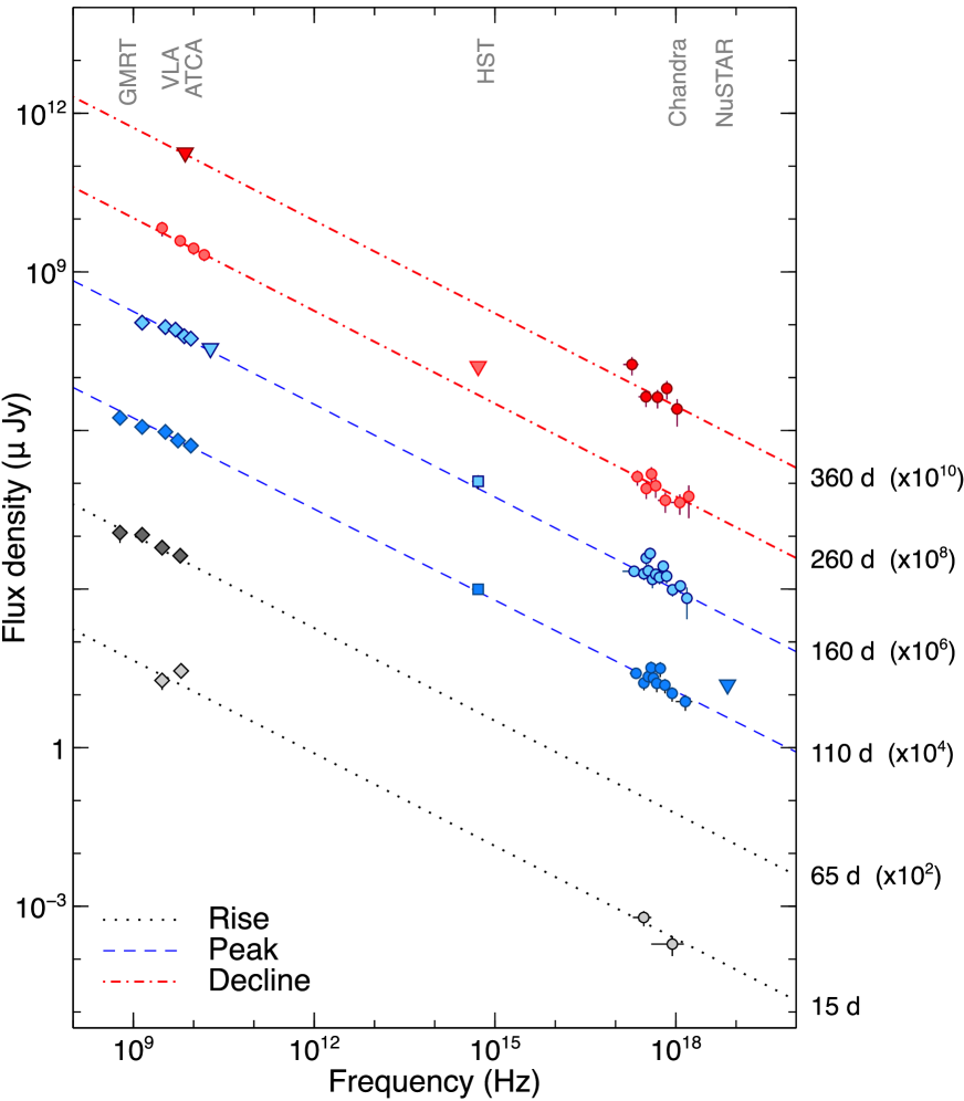
Figure 1: Temporal evolution of the afterglow spectral energy distribution. A single power-law segment can describe the broadband spectrum during the different afterglow phases (rise, peak and decline). At all times, a simple power-law model provides a good fit of the data.

2.1 Spectral properties

The latest epoch of X-ray observations shows a simple power-law spectrum with index $\beta$=0.8$\pm$0.4, consistent with previous measurements, and with the spectral index 0.4$\pm$0.3 from the late time ($t>$220 d) radio data. Figure 1 shows that, at all epochs, the broadband spectrum can be fit with a simple power-law model with spectral index $\beta$=0.585$\pm$0.005 and no intrinsic absorption in addition to the Galactic value $N_{H}$=7.6$\times$10²⁰ cm^-2. The lack of any significant spectral variation on such long timescales is remarkable. In GRB afterglows, a steepening of the X-ray spectrum due to the gradual decrease of the cooling frequency $\nu_{c}$ is commonly detected within a few days. Since the cooling break is a smooth spectral feature, we used a curved afterglow spectrum (Granot & Sari, 2002) to fit the data, and constrain its location. We derived $\nu_{c}\gtrsim$1 keV (90% confidence level) at 260 d after the merger and $\nu_{c}\gtrsim$0.1 keV (90% confidence level) at 360 d.

For a synchrotron spectrum with $\nu_{m}<\nu_{obs}<\nu_{c}$, the measured spectral index is related to the spectral index $p$ of the emitting electrons (e.g. Granot & Sari, 2002) as $p$ = 2$\beta$ +1 = 2.170 $\pm$ 0.010. Figure 2 compares this value with a sample of well-constrained short and long GRB spectra. It shows that, among short GRB spectra, GW170817/GRB170817A represents the most precise measurement obtained so far. Such precision is rare, but not unprecedented among long GRB afterglows.

It is tempting to interpret the accurately determined value of $p$ as an intermediate between relativistic and non-relativistic shock acceleration, based on theoretical considerations of plausible mechanisms (Kirk et al., 2000; Achterberg et al., 2001; Spitkovsky, 2008), implying $\Gamma$ $\approx$2-10 for the emitting material (Margutti et al., 2018). On the other hand, various well constrained short GRB $p$-values lie outside this theoretical range (Fig. 2), the $p$-value distribution for the larger sample of (long) GRBs does not appear consistent with a universal value for $p$ (Shen et al., 2006; Curran et al., 2010), nor is there generally any evidence for evolution of $p$ from multi-epoch spectral energy distributions (SEDs) (Fig. 1, also e.g. Varela et al. 2016) or light curve slopes. In view of these features of the general sample of long and short GRBs (as well as other synchrotron sources, such as blazars), direct interpretation of $p\approx 2.17$ in terms of shock-acceleration theory might be premature.

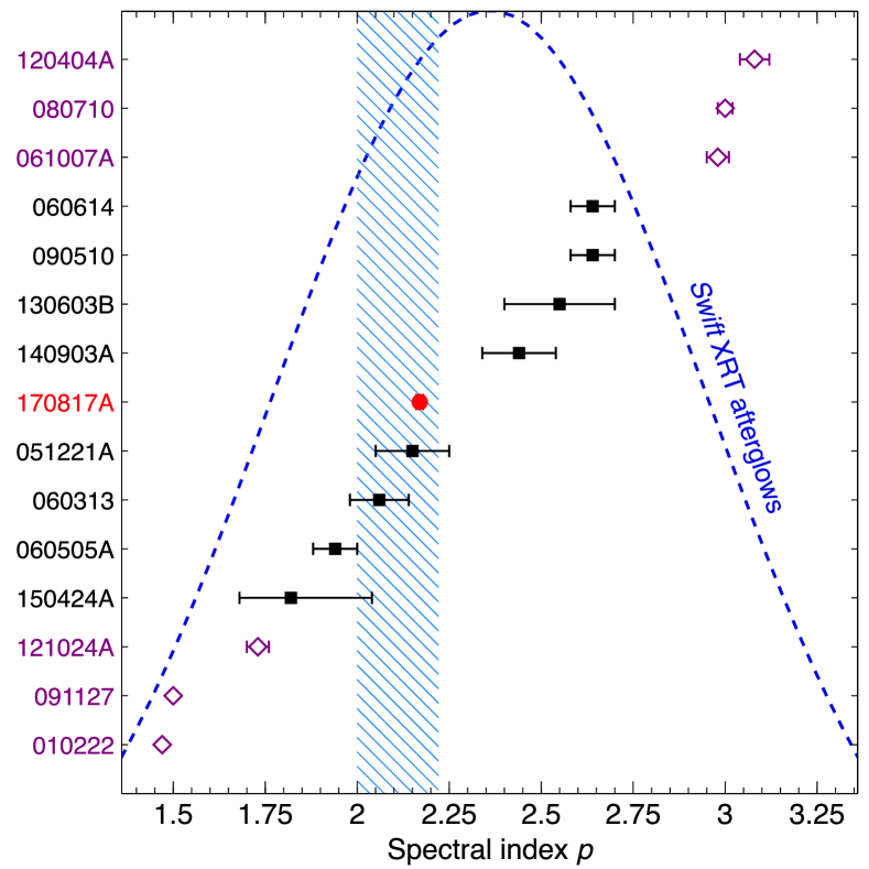
Figure 2: Spectral index $p$ of the shock-accelerated electrons for GW170817/GRB170817A (filled circle) and a sample of of short GRBs (filled squares) and long GRBs (open diamonds) with good afterglow constraints. The dashed line shows the distribution inferred from XRT afterglows (Curran et al., 2010). The hatched area shows the range of values predicted by shock theory. Data are from: Roming et al. (2006); Soderberg et al. (2006); Mundell et al. (2007); Resmi & Bhattacharya (2008); Xu et al. (2009); Krühler et al. (2009); Kumar & Barniol Duran (2010); Troja et al. (2012, 2016); Fong et al. (2015); Varela et al. (2016); Knust et al. (2017).

2.2 Temporal properties

We simultaneously fit the multi-color (X-ray, optical, radio) light curves by adopting a simple power-law function in the spectral domain, and a smoothly broken power-law in the temporal domain (Beuermann et al., 1999). The functional form is: $F(\nu,t)\propto\nu^{-\beta}\left[(t/t_{p})^{-\kappa\alpha_{1}}+(t/t_{p})^{\kappa\alpha_{2}}\right]^{-1/\kappa}$, where $\beta$ is the spectral index, $\alpha_{1}$ and $\alpha_{2}$ are the rise and decay slopes, $t_{p}$ is the peak time, and $\kappa$ is the smoothness parameter.

We did not impose an achromatic behavior. Instead, the temporal properties were modeled as a hierarchy where the parameters for each wavelength have an independent value, sampled from a hyper distribution. Variations in the hierarchy would be integrated out of the posterior if justified by the data.

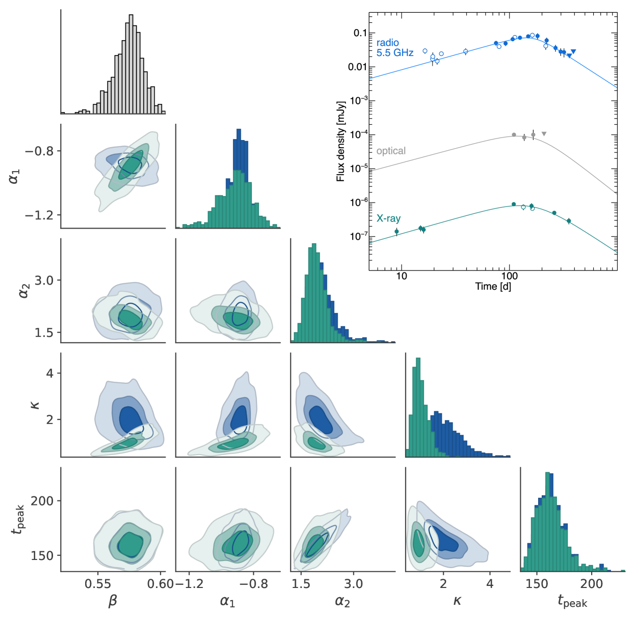
Figure 7: Corner plot for the empirical model described in Sect. 2.2. The prior on each of these parameters is normal, the center and standard deviation were: $\beta$ = (1,1), $\alpha_{1}$ = (0.5,1), $\alpha_{2}$ = (-2.5,1), log $\kappa$ = (0,0.5), log $t_{\rm peak}$ = (2,2). We report the confidence contours derived from radio (blue) and X-ray (green) data, as the optical light curve is only poorly constrained. The best fit model is shown in the top-left corner.

Scale-family distributions were given log-normal priors and all other parameters were given normal priors. To fit the model, we employ the NUTS variant of Hamiltonian Monte Carlo via the Stan modeling language (Carpenter et al., 2017). The peak time and rise slope are well constrained to $t_{p}$=164$\pm$12 d and $\alpha_{1}$=0.90$\pm$0.06. Whereas the optical afterglow is poorly sampled, the X-ray and radio light curves allow for better constraints on the decay slope, $\alpha_{2}$=2.0${}^{+0.8}_{-0.5}$ (Figure 3), and are both consistent with a rapid decline of the afterglow flux. The best fit model and full corner plot is reported in the Supplementary Material (Figure 7).

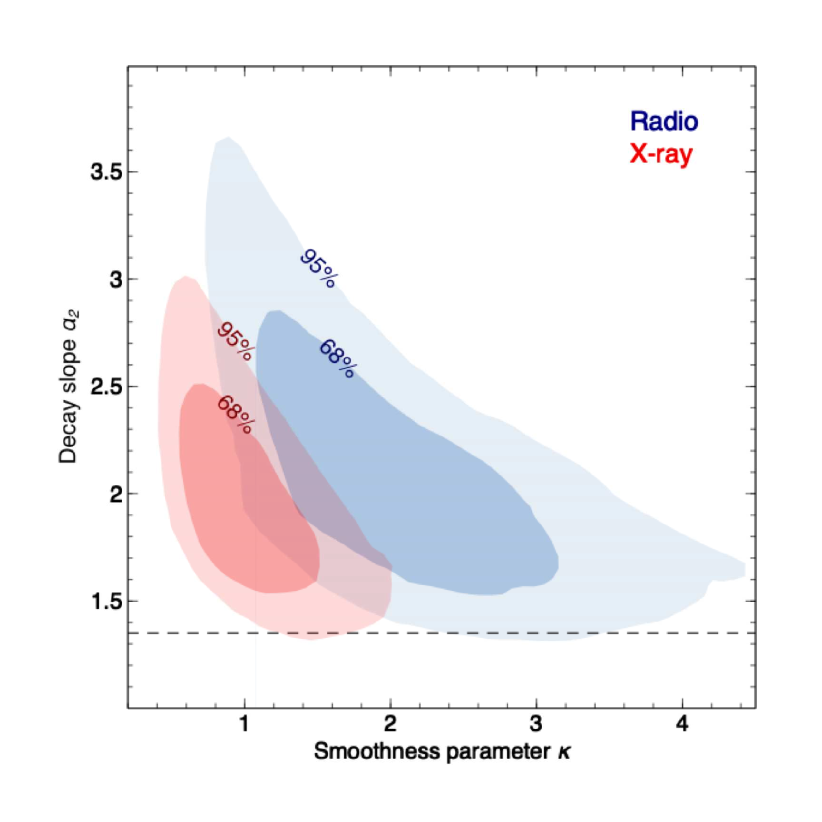
Figure 3: Joint marginal distribution of the decay index ($\alpha_{2}$) and smoothness parameter ($s$) for the radio (blue) and X-ray (red) light curves. The dashed line corresponds to $\alpha_{2}=1.35$, the steepest value predicted by choked jet/cocoon models.

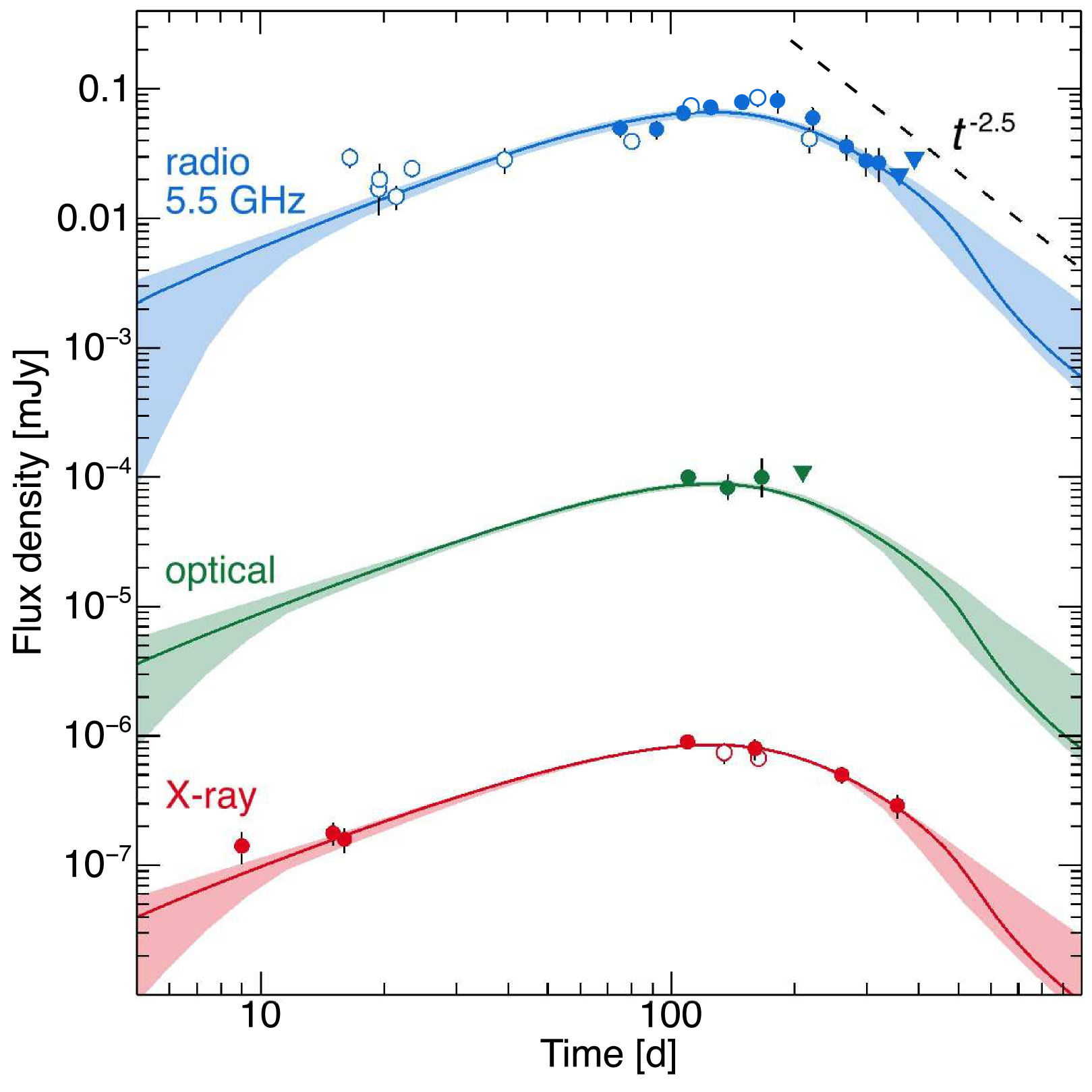
Figure 4: Multi-wavelength afterglow light curves overlaid with the Gaussian jet best fit model (solid line) and its 68% uncertainty range (shaded areas). Radio data are from ATCA (filled symbols) and VLA (open symbols) observations. X-ray data are from Chandra (filled symbols) and XMM-Newton (open symbols) observations. Downward triangles are 3 $\sigma$ upper limits. The dashed line shows the expected asymptotic decline $\propto t^{-2.5}$. Data were collected from: Troja et al. 2017, Troja et al. 2018a, Piro, et al. 2019, Hallinan et al. 2017, Lyman et al. 2018, Resmi, et al. 2018, Margutti et al. 2018, Mooley et al. 2018a, and Alexander et al. 2018.

2.3 Modeling

We directly fit two semi-analytical models for structured outflows to the data, following the description in Troja et al. (2018a). The off-axis structured jet model assumes a Gaussian energy profile $E\propto\exp\left(-\theta^{2}/2\theta_{c}^{2}\right)$ up to a truncating angle $\theta_{w}$. The jet is fully determined by a set of eight parameters $\Theta_{\mathrm{jet}}=\{E_{0},n,\epsilon_{e},\epsilon_{B}\,p,\theta_{c},\theta_{w},\theta_{v}\}$, where $E_{0}$ is the on-axis isotropic-equivalent kinetic energy of the blast wave, $n$ the circumburst density, $\epsilon_{e}$ the electron energy fraction, $\epsilon_{B}$ the magnetic energy fraction and $\theta_{v}$ the angle between the jet-axis and the observer’s line of sight. Following Mooley et al. (2018a), we also fit a cocoon model with a velocity stratification of the ejecta to allow for a slower rise and late turnover. The total amount of energy in the slower ejecta above a particular four-velocity $u$ is modelled as a power-law $E(>u)=E_{\mathrm{inj}}u^{-k}$. This model requires nine parameters $\Theta_{\mathrm{cocoon}}=\{E_{\mathrm{inj}},n,p,\epsilon_{e},\epsilon_{B}\,M_{\mathrm{ej}},u_{\mathrm{max}},u_{\mathrm{min}},k\}$, where $u_{\mathrm{max}}$ is the maximum ejecta four-velocity, $u_{\mathrm{min}}$ the minimum ejecta four-velocity, and $M_{\mathrm{ej}}$ the initial cocoon ejecta mass with speed $u_{\mathrm{max}}$.

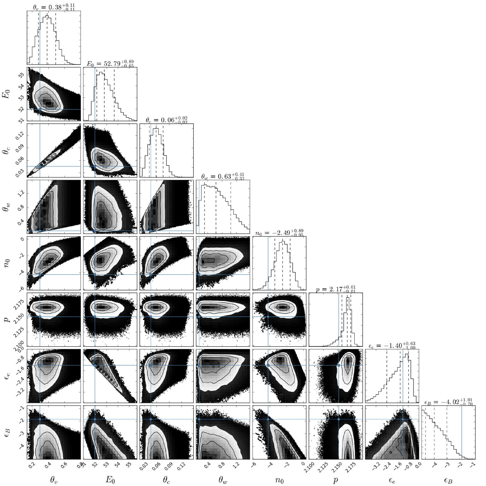
Figure 8: Fit result for the Gaussian jet model. This “corner plot” shows all one-dimensional (diagonal) and two-dimensional (off-diagonal) projections of the posterior probability density function. The best-fit value (maximum posterior probability) is shown in blue. Dotted lines mark the 16%, 50%, and 84% quantiles of the marginalized posteriors for each parameter.

As described in Troja et al. (2018a), our Bayesian fit procedure utilizes the emcee Markov-chain Monte Carlo package (Foreman-Mackey et al., 2013). For the structured jet we also include the GW constraints on the orientation $\iota$ of the system (Abbott et al., 2017b) in our prior for $\theta_{v}$. The results of the MCMC analysis are summarized in Table 2. The best fit jet models is shown in Figure 4. For the corner plot see the Supplementary data (Figure 8).

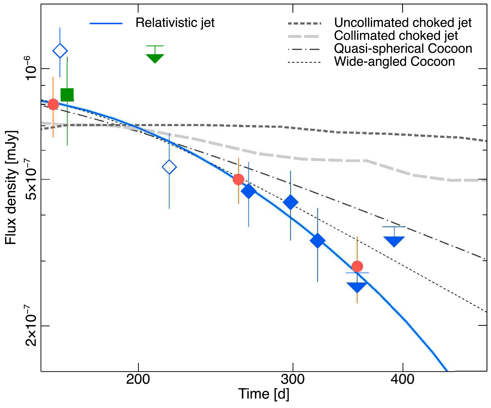
Figure 5: Late time afterglow light curves compared to different explosion models: choked jets from numerical simulations (thicker lines, Nakar, et al. 2018), wide-angled cocoon (Lamb, Mandel & Resmi, 2018), and our best fit models of quasi-spherical cocoon (dot-dashed line) and structured jet (solid line). Different symbols represent different wavelengths: X-rays (circles), optical (downward triangles; 3 $\sigma$ upper limits), and radio (diamonds) from ATCA (filled) and VLA (empty). For plotting purposes, data were rescaled to a common energy of 5 keV using the observed spectral slope $\beta$=0.585.

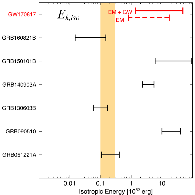
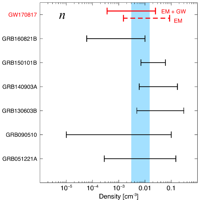
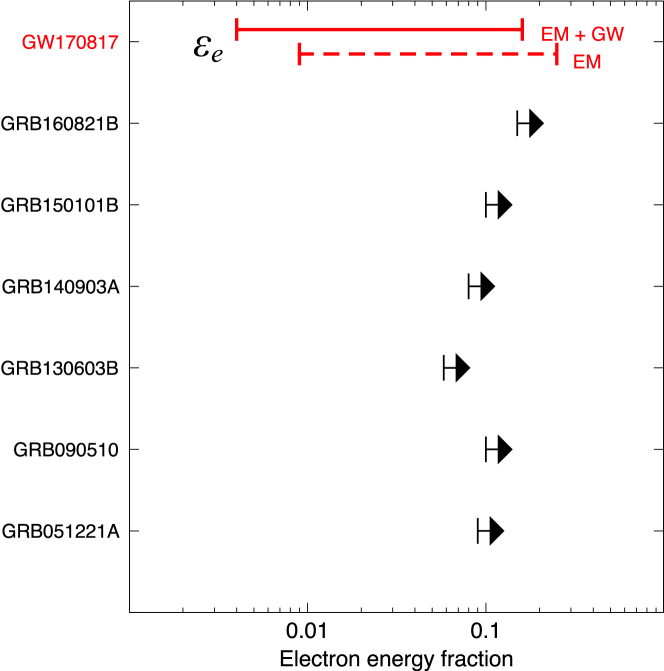
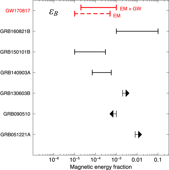
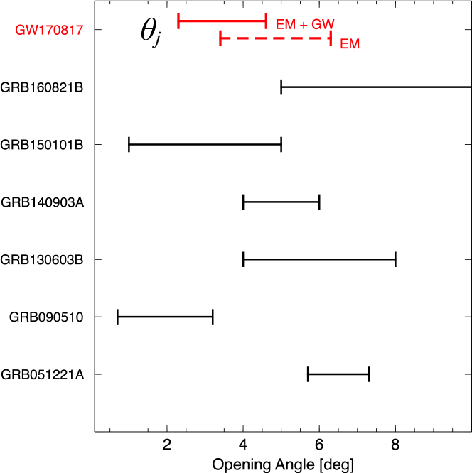
Figure 6: Afterglow parameters for GW170817 and a sample of cosmological ($z>$0.1) short GRBs with multi-wavelength afterglows. For GW170817 we report the results based purely on the electromagnetic observations (EM), and those incorporating the LIGO constraints on the binary inclination (EM+GW). Data are from: Soderberg et al. (2006); Kumar & Barniol Duran (2010); Fong et al. (2015); Troja et al. (2016, 2018b); Troja, et al. (2019) The vertical grey band show the median values of energy $E_{k,\rm iso}$ and density $n$ for the larger sample of Swift short GRBs (Fong et al., 2015).

3 Results

3.1 A rapid afterglow decline: constraints on the outflow structure

For jets that fail to break out (“choked jets”), the jet energy is dissipated into a surrounding cocoon of material. This scenario is therefore included in our group of ‘cocoon’ models (Troja et al., 2018a). The post-peak temporal slope is a shallow decay of $\alpha\approx 1.0-1.2$ up to at least 300 days for GRB 170817A, as can be inferred from semi-analytical modeling of the evolution of a trans-relativistic shell (Troja et al., 2018a). Any remaining post-turnover impact due to continued energy injection from e.g. a complex velocity profile of the ejecta, would lead to an even shallower decay. Afterwards, the slope will eventually become that of an expanding non-relativistic (quasi-)spherical shell. As for the Sedov-Taylor solution of a point explosion in a homogeneous medium, this slope translates to $\alpha=(15p-21)/10$ for $\nu_{m}<\nu_{obs}<\nu_{c}$, when combined with a standard synchrotron model for shock-accelerated electrons (Frail et al., 2000). The value $p\approx 2.17$ implies $\alpha\approx 1.155$. If $\nu_{m},\nu_{c}<\nu_{obs}$, $\alpha=(3p-4)/2\approx 1.255$ instead (e. g. Granot & Sari, 2002). If the cocoon choking the jet is not quasi-spherical, but merely wide-angled, some sideways spreading of the outflow may still occur. By definition for a non-relativistic flow velocity, this will not produce any observational features related to relativistic beaming, but the continuous increase in working surface will give rise to additional deceleration of the blast wave relative to the case of purely radial flow. As a result, the temporal slope could steepen slightly by another $\Delta\alpha\approx 0.15-0.2$ (Lamb, Mandel & Resmi, 2018), before settling into the late quasi-spherical stage. For GW170817, this implies a maximum $\alpha\approx 1.35$ from a cocoon-dominated / choked jet model.
By contrast, if the jet has a relativistically moving inner region (in terms of angular distribution of Lorentz factor), the post-peak temporal slope will be like that of an on-axis jet seen after the jet break: the entire surface of the jet has come into view and there is no longer a contribution to the light curve slope from a growing visible patch. Different calculations predict various degrees of steepening (e.g. Gill & Granot, 2018): a slope $\alpha\approx p$ according to analytical models (Sari et al., 1999), and a somewhat steeper $\alpha\approx 2.5$ according to semi-analytical models (Troja et al., 2018a) and hydrodynamical simulations of jets (van Eerten & MacFadyen 2013, although the latter were done for jets starting from top-hat initial conditions).

As derived in section 2.2, the decay slope $\alpha_{2}$ of the empirical model exceeds the predictions of most choked jet models by a healthy margin. This is confirmed by the comparison of the late afterglow data, from radio to X-rays, with physical models of choked and structured jets (Figure 5). The observed decay is consistent with the turnover of a structured jet (solid line). While the observed $\alpha_{2}$ is not as steep as $2.5$, this is not unexpected for a jetted flow as the transition of the light curve from rise to decay is spread out over time (and fully captured by the direct application of a structured jet model in section 2.3, see also Fig. 4).

The rapid decline of the afterglow therefore poses an additional challenge to the choked jet models, in support to the results of the high-resolution radio imaging (Mooley et al., 2018b; Ghirlanda, et al., 2019). While growing evidence indicates that the merger remnant launched a successful relativistic jet, the presence of a cocoon cannot be excluded. There might well be an observable cocoon component present in the outflow even for successful jets (Nagakura et al., 2014; Murguia-Berthier et al., 2014). Indeed, the structured jet itself might be an indication of the presence of a cocoon (in case the structure is not imposed by the torus upon launching, Aloy et al. 2005). However, it would appear any such cocoon is not the dominant emission component at late times.

3.2 Afterglow properties: comparison to short GRBs

The predictive power of each model can be judged by the deviance information criteria (DIC), where lower scores correspond to greater predictive power (Spiegelhalter et  al., 2002). The Gaussian jet model fit has a DIC of 103.5 and the cocoon model fit has a DIC of 151.8, favoring the Gaussian jet as the more predictive model. For all models and priors, the posterior value of the electron power law slope lies around $p=2.170\pm 0.010$, fully consistent with the value obtained by the spectral analysis (Section 2.1).

The cocoon model requires a small amount of relativistic ejecta with a substantial Lorentz factor $\Gamma_{max}\in[6.1,200]$ (all ranges with 68% percent confidence) followed by an energetic tail of slower ejecta with minimum Lorentz factor $\Gamma_{min}\in[1.9,7.48]$. The high Lorentz factors are in tension with a choked-jet scenario, where the ejecta achieve only Newtonian velocity. The total energy, assuming a spherical blast wave, is rather high, between $10^{51}$ and $4\times 10^{53}$ erg. The circumburst density and shock micro-physical parameters are very poorly constrained in this model.

The Gaussian jet (Figure 4) has a well constrained width $\theta_{c}$ = 0.06$\pm$0.02 rad (3.4^∘ $\pm$ 1.1^∘), and a total energy between $5\times 10^{49}$ and $1.4\times 10^{51}$ erg. The wide truncation angle is largely unconstrained. The ambient density $n$ is constrained to be between $3\times 10^{-4}$ and $2.4\times 10^{-2}$ cm^-3. The micro-physical parameters $\epsilon_{e}\in[4\times 10^{-3},0.17]$ and $\epsilon_{B}\in[2.7\times 10^{-5},10^{-3}]$ are only somewhat constrained by the model fit. The constraint $\nu_{c}>$ 1 keV from the lack of spectral steepening drives the relatively small value for $\epsilon_{B}$, as $\nu_{c}\propto\epsilon_{B}^{-3/2}$. These values were derived by assuming a jet with a Gaussian angular profile, yet they are in good agreement with other estimates based on different angular structures (e.g. Ghirlanda, et al., 2019).

The viewing angle derived from the electromagnetic observations alone is 0.52$\pm$0.16 rad (30^∘ $\pm$ 9^∘), consistent with the constraints from prompt emission (e.g Abbott et al., 2017a; Bégué et al., 2017), optical and radio imaging (Mooley et al., 2018b; Ghirlanda, et al., 2019; Lamb, et al., 2019). By adding the GW constraints on the binary inclination $\iota$ to our modeling, we obtain $\theta_{v}$ = 0.38$\pm$0.11 rad (22^∘ $\pm$ 6^∘), consistent with the LIGO estimates that informed the prior. The good agreement of the electromagnetic and GW constraints suggest that the relativistic jet was launched nearly perpendicularly to the orbital plane.

The year-long monitoring of GW170817 significantly reduced the allowed parameter space of models, tightening the constraints on the afterglow properties. This allows for a comparison with other well-studied short GRB explosions, as presented in Figure 6. It is remarkable how the properties of GW170817 fit within the range of short GRB afterglows. The low circumburst densities $n\approx$0.01 cm^-3 are typical of the interstellar medium, and consistent with the location of these bursts within their galaxy light. The electron energy fraction seems well constrained to $\epsilon_{e}\gtrsim$0.1, whereas $\epsilon_{B}$ tends to lower values $\lesssim$0.01, and is only loosely constrained. The narrow width of the Gaussian jet $\theta_{c}$ of GW170817 is comparable to the half-opening angle $\theta_{j}$ inferred from top-hat jet models of short GRBs (e.g. Troja et al., 2016), suggesting that these GRB jets had narrow cores of similar size. The isotropic-equivalent energy is also consistent with the measurements from other short GRBs, although we note that most events in the sample lie above the median value of $E_{k,iso}$ (vertical band). This is not surprising as we selected the cases of well-sampled light curves with good afterglow constraints, thus creating a bias toward the brightest explosions.

4 Conclusions

The long-term afterglow monitoring of GW170817 supports the earlier suggestions of a relativistic jet emerging from the merger remnant, and challenges the alternative scenarios of a choked jet. Whereas emission at early times ($<$160 d) came from the slower and less energetic lateral wings, the rapid post-peak decline suggests that emission from the narrow jet core has finally entered our line of sight. The overall properties of the explosion, as derived from the afterglow modeling, are consistent with the range of properties observed in short GRBs at cosmological distances, and suggest that we detected its electromagnetic emission thanks to a combination of moderate off-axis angle ($\theta_{v}$-$\theta_{c}$ $\approx$20^∘ ) and intrinsic energy of the explosion.

Table 1: Late-time X-ray and radio observations of GW170817

T-T0	Facility	Exposure	$\beta$	Flux	Frequency
(d)				($\mu$Jy)	(GHz)
267	ATCA	11.0h	0.8$\pm$0.8	30$\pm$7	5.5
				20$\pm$6	9.0
				30$\pm$6	7.25
298	ATCA	11.0h	-0.3$\pm$1.0	25$\pm$7	5.5
				29$\pm$6	9.0
				28$\pm$6	7.25
320	ATCA	11.5h	0.4$\pm$0.8	27$\pm$8	5.5
				22$\pm$6	9.0
				22$\pm$5	7.25
359	ATCA	9.5h	$--$	$<$26	5.5
				$<$20	9.0
				$<$18	7.25
391	ATCA	9.5h	$--$	$<$33	5.5
				$<$27	9.0
				$<$24	7.25
359	Chandra	67.2 ks	0.8$\pm$0.4	2.8${}^{+0.3}_{-0.5}$ $\times$ 10-4	1.2$\times$109
			0.585	2.1${}^{+0.2}_{-0.3}$$\times$ 10-4	1.2$\times$109

Table 2: Constraints on the Gaussian jet and Cocoon model parameters. Reported are the median values of each parameter’s posterior distribution with symmetric 68% uncertainties (ie. the 16% and 84% quantiles). The first Gaussian jet column uses constraints from the afterglow alone, the second includes the LIGO constraints on the inclination angle using the Planck value of $H_{0}$.

Parameter Jet Jet+GW+Planck $\theta_{v}$ $0.52^{+0.16}_{-0.16}$ $0.38^{+0.11}_{-0.11}$ $\log_{10}E_{0}$ $52.47^{+0.81}_{-0.56}$ $52.80^{+0.89}_{-0.65}$ $\theta_{c}$ $0.079^{+0.026}_{-0.024}$ $0.059^{+0.017}_{-0.017}$ $\theta_{w}$ $0.77^{+0.47}_{-0.38}$ $0.61^{+0.42}_{-0.31}$ $\log_{10}n$ $-1.83^{+0.77}_{-1.0}$ $-2.51^{+0.90}_{-0.99}$ $p$ $2.1678^{+0.0064}_{-0.010}$ $2.1681^{+0.0062}_{-0.0095}$ $\log_{10}\epsilon_{e}$ $-1.13^{+0.53}_{-0.88}$ $-1.39^{+0.62}_{-0.99}$ $\log_{10}\epsilon_{B}$ $-4.18^{+0.85}_{-0.58}$ $-4.00^{+1.0}_{-0.69}$ $\log_{10}E_{tot}$ $50.24^{+0.72}_{-0.47}$ $50.30^{+0.84}_{-0.57}$

Parameter Cocoon $\log_{10}u_{\mathrm{max}}$ $1.38^{+0.92}_{-0.6}$ $\log_{10}u_{\mathrm{min}}$ $0.51^{+0.36}_{-0.29}$ $\log_{10}E_{\mathrm{inj}}$ $56.1^{+3.2}_{-2.9}$ $k$ $7.26^{+0.41}_{-0.57}$ $\log_{10}M_{\mathrm{ej}}$ $-8.2^{2.0}_{-1.3}$ $\log_{10}n$ $-4.5^{+2.1}_{-2.4}$ $p$ $2.1715^{+0.0055}_{-0.0057}$ $\log_{10}\epsilon_{e}$ $-2.0^{+1.3}_{-1.3}$ $\log_{10}\epsilon_{B}$ $-3.4^{+1.7}_{-1.1}$ $\log_{10}E_{tot}$ $52.4^{+1.2}_{-1.3}$

References

- Abbott et al. (2017a) Abbott B. P., et al., 2017a, ApJL, 848, L13
- Abbott et al. (2017b) Abbott B. P., et al., 2017b, Nature, 551, 85
- Achterberg et al. (2001) Achterberg A., Gallant Y. A., Kirk J. G., Guthmann A. W., 2001, MNRAS, 328, 393
- Alexander et al. (2018) Alexander K. D., et al., 2018, preprint, arXiv 1805.02870
- Aloy et al. (2005) Aloy M. A., Janka H.-T., Müller E., 2005, A&A, 436, 273
- Bégué et al. (2017) Bégué D., Burgess J. M., Greiner J., 2017, ApJ, 851, L19
- Beuermann et al. (1999) Beuermann, K., Hessman, F. V., Reinsch, K., et al. 1999, A&A, 352, L26
- Carpenter et al. (2017) Carpenter B., et al., 2017, Journal of Statistical Software, Vol. 76, Issue 1, 2017, 76
- Corsi et al. (2018) Corsi A., et al., 2018, ApJL, 861, L10
- Curran et al. (2010) Curran P. A., Evans P. A., de Pasquale M., Page M. J., van der Horst A. J., 2010, ApJL, 716, L135
- D’Avanzo et al. (2018) D’Avanzo P., et al., 2018, A&A, 613, L1
- Fong et al. (2015) Fong W., Berger E., Margutti R., Zauderer B. A., 2015, ApJ, 815, 102
- Foreman-Mackey et al. (2013) Foreman-Mackey D., Hogg D. W., Lang D., Goodman J., 2013, PASP, 125, 306
- Frail et al. (2000) Frail D. A., Waxman E., Kulkarni S. R., 2000, ApJ, 537, 191
- Ghirlanda, et al. (2019) Ghirlanda G., et al., 2019, Sci, 363, 968
- Gill & Granot (2018) Gill R., Granot J., 2018, MNRAS, 478, 4128
- Granot & Sari (2002) Granot J., Sari R., 2002, ApJ, 568, 820
- Haggard et al. (2017) Haggard, D., Nynka, M., Ruan, J. J., et al. 2017, ApJ, 848, L25
- Hallinan et al. (2017) Hallinan G., et al., 2017, Science, 358, 1579
- Kasliwal et al. (2017) Kasliwal M. M., et al., 2017, Science, 358, 1559
- Kathirgamaraju et al. (2018) Kathirgamaraju A., Barniol Duran R., Giannios D., 2018, MNRAS, 473, L121
- Kirk et al. (2000) Kirk J. G., Guthmann A. W., Gallant Y. A., Achterberg A., 2000, ApJ, 542, 235
- Knust et al. (2017) Knust F., et al., 2017, A&A, 607, A84
- Krühler et al. (2009) Krühler T., et al., 2009, A&A, 508, 593
- Kumar & Barniol Duran (2010) Kumar P., Barniol Duran R., 2010, MNRAS, 409, 226
- Lamb, Mandel & Resmi (2018) Lamb G. P., Mandel I., Resmi L., 2018, MNRAS, 481, 2581
- Lamb, et al. (2019) Lamb G. P., et al., 2019, ApJL, 870, L15
- Lazzati et al. (2017) Lazzati D., López-Cámara D., Cantiello M., Morsony B. J., Perna R., Workman J. C., 2017, ApJ, 848, L6
- Lazzati et al. (2018) Lazzati D., Perna R., Morsony B. J., Lopez-Camara D., Cantiello M., Ciolfi R., Giacomazzo B., Workman J. C., 2018, [Physical Review Letters], 120, 241103
- Lyman et al. (2018) Lyman J. D., et al., 2018, Nature Astronomy
- Margutti et al. (2018) Margutti R., et al., 2018, ApJL, 856, L18
- Mooley et al. (2018a) Mooley K. P., et al., 2018a, Nature, 554, 207
- Mooley et al. (2018b) Mooley K. P., et al., 2018b, Nature, 561, 355
- Mundell et al. (2007) Mundell C. G., et al., 2007, ApJ, 660, 489
- Murguia-Berthier et al. (2014) Murguia-Berthier A., Montes G., Ramirez-Ruiz E., De Colle F., Lee W. H., 2014, ApJ, 788, L8
- Nagakura et al. (2014) Nagakura H., Hotokezaka K., Sekiguchi Y., Shibata M., Ioka K., 2014, ApJL, 784, L28
- Nakar, et al. (2018) Nakar E., Gottlieb O., Piran T., Kasliwal M. M., Hallinan G., 2018, ApJ, 867, 18
- Piro, et al. (2019) Piro L., et al., 2019, MNRAS, 483, 1912
- Planck Collaboration et al. (2018) Planck Collaboration et al., 2018, preprint, arXiv 1807.06209
- Resmi & Bhattacharya (2008) Resmi L., Bhattacharya D., 2008, MNRAS, 388, 144
- Resmi, et al. (2018) Resmi L., et al., 2018, ApJ, 867, 57
- Roming et al. (2006) Roming P. W. A., et al., 2006, ApJ, 651, 985
- Sari et al. (1999) Sari R., Piran T., Halpern J. P., 1999, ApJ, 519, L17
- Shen et al. (2006) Shen R., Kumar P., Robinson E. L., 2006, MNRAS, 371, 1441
- Soderberg et al. (2006) Soderberg A. M., et al., 2006, ApJ, 650, 261
- Spiegelhalter et al. (2002) Spiegelhalter D. J., 2002, JRAS, 64, 583
- Spitkovsky (2008) Spitkovsky A., 2008, ApJ, 682, L5
- Troja et al. (2012) Troja E., et al., 2012, ApJ, 761, 50
- Troja et al. (2016) Troja E., et al., 2016, ApJ, 827, 102
- Troja et al. (2017) Troja E., et al., 2017, Nature, 551, 71
- Troja et al. (2018a) Troja E., et al., 2018a, MNRAS, 478, L18
- Troja et al. (2018b) Troja E., et al., 2018b, Nature Communications, 9, 4089
- Troja, et al. (2019) Troja E., et al., 2019, arXiv, arXiv:1905.01290
- Varela et al. (2016) Varela K., et al., 2016, A&A, 589, A37
- Xie et al. (2018) Xie X., Zrake J., MacFadyen A., 2018, ApJ, 863, 58
- Xu et al. (2009) Xu D., et al., 2009, ApJ, 696, 971
- van Eerten & MacFadyen (2013) van Eerten H., MacFadyen A., 2013, ApJ, 767, 141