A HIGH CLUSTER FORMATION EFFICIENCY IN THE SAGITTARIUS B2 COMPLEX

Abstract

The fraction of stars forming in compact, gravitationally bound clusters (the ‘cluster formation efficiency’ or CFE) is an important quantity for deriving the spatial clustering of stellar feedback and for tracing star formation using stellar clusters across the Universe. Observations of clusters in nearby galaxies have revealed a strong dependence of the CFE on the local gas density, indicating that more stars form in star clusters when the star formation rate surface density is higher. Previously, it has not been possible to test this relation at very young ages and in clusters with individual stars resolved due to the universally-low densities in the cluster-forming regions in the Local Group. This has even led to the suggestion that the CFE increases with distance from the Sun, which would suggest an observational bias. However, the Central Molecular Zone of the Milky Way hosts clouds with densities that are orders of magnitude higher than anywhere else in the Local Group. We report a measurement of the CFE in the highest-density region in the Galaxy, Sgr B2, based on ALMA observations of high-mass young stellar objects. We find that over a third of the stars ($37\pm 7\%$) in Sgr B2 are forming in bound clusters. This value is consistent with the predictions of environmentally-dependent models for the CFE and is inconsistent with a constant CFE in the Galaxy.

doublespace

1 Introduction

Gravitationally bound stellar clusters are some of the most important objects in astronomy, providing both luminous probes of the star formation process at great distances (e.g., Brodie & Strader, 2006; Adamo et al., 2013; Kruijssen et al., 2018a, b, among many others) and large coeval and co-located samples of stars in the local universe. The prevalence of these clusters varies substantially with environment: the fraction of star formation occurring in bound, compact clusters, i.e., the cluster formation efficiency (CFE) $\Gamma$ is not constant (Adamo et al., 2015; Johnson et al., 2016; Messa et al., 2018).

Kruijssen (2012) proposed a theory in which $\Gamma$ is a function of gas density, with secondary dependences on other global environmental quantities. While this theory reasonably explains observations spanning many galaxies, it has not yet been directly tested in a high-density environment where both the unclustered and clustered stars are detected in a spatially resolved sense. In this Letter, we perform such a test in the Sgr B2 cloud, a high-density region in the Galactic center in which both stars and compact clusters (taken to be a proxy for gravitational boundedness) are presently forming.

2 Census of the Stellar Population

We use the catalogs of millimeter and centimeter sources described in Ginsburg et al. (2018), Gaume et al. (1995), and De Pree et al. (2015), which consist of candidate young high-mass stars and young stellar objects (YSOs), to infer the total stellar population in Sgr B2.

Gaume et al. (1995) observed Sgr B2 at 1.3 cm with $\sim 0.25$″ resolution with the VLA. They detected 49 continuum sources. These are exclusively H ii regions and components of H ii regions. De Pree et al. (2015) used 7 mm JVLA Q-band observations at 0.05″ resolution to catalog 26 sources in Sgr B2 M and 5 in Sgr B2 N. Of these, 7 detected in Sgr B2 M were not reported in Gaume et al. (1995) because they were not resolved. We assume each of the VLA-detected sources is an H ii region and therefore contains at least one star with $M\gtrsim 20$ $\mathrm{M}_{\odot}$, equivalent to a B0 star.

Ginsburg et al. (2018) observed the cloud with ALMA, obtaining a resolution of $0.5\arcsec$ in the 3 mm band. They reported a total of 271 sources spread throughout the cloud, of which 31 are confirmed H ii regions with implied masses $M_{*}>20$ $\mathrm{M}_{\odot}$; the rest are YSO candidates with masses $M_{*}>8$ $\mathrm{M}_{\odot}$. We follow Ginsburg et al. (2018) in extrapolating the total stellar mass implied by the observed objects using a Kroupa (2001) initial mass function. With this extrapolation, each H ii region implies the presence of a total of 326 $\mathrm{M}_{\odot}$ of stars, while each 8-20 $\mathrm{M}_{\odot}$ core represents 135 $\mathrm{M}_{\odot}$, assuming an upper stellar mass limit of 200 $\mathrm{M}_{\odot}$ (though these numbers are weakly sensitive to the upper mass limit).

3 Mass of the clusters

In Table 2 of Ginsburg et al. (2018), four clusters are considered: N, M, NE, and S. Here, we re-evaluate the “clusters” in NE and S. These regions contain few sources and are not centrally concentrated. They are both moderate mass and, at present, are not guaranteed to form bound clusters based on their irregular morphology. We therefore exclude them from the analysis, but note that if they are forming bound clusters, the measured CFE would increase by a few percent. Our census of star and cluster formation is summarized in Table 1.

Table 1: Cluster Masses

Name	$N({\rm cores})$	$N({\rm H\textsc{ii}})$	$M_{\rm inferred,cores}$	$M_{\rm inferred,H\textsc{ii}}$	$M_{\rm inferred,max}$
			$\mathrm{M_{\odot}}$	$\mathrm{M_{\odot}}$	$\mathrm{M_{\odot}}$
M	17	47	2300	15000	15000
N	11	3	1500	980	1500
NE	4	0	540	0	540
S	5	1	680	330	680
Unassociated	203	6	27000	2000	27000
Total	240	57	33000	19000	46000
Clustered with NE, S	37	51	5000	17000	18000
Clustered only M, N	28	50	3800	16000	17000

Partial reproduction of Table 2 in Ginsburg et al. (2018). $M_{\rm inferred,cores}$ and $M_{\rm inferred,\textup{H\,{ii}}}$ are the inferred total stellar masses assuming the counted objects represent fractions of the total mass of 0.09 (cores) and 0.14 (H ii regions). $M_{\rm inferred,max}$ is the greater of these two. The Total row represents the total over the whole observed region. The two Clustered rows show the total inferred mass of clusters including all four candidate clusters M, N, NE and S, then the mass of clusters including only M and N.

3.1 Cluster membership in Sgr B2 M

Schmiedeke et al. (2016) marked the Sgr B2 M cluster as a 13″ (0.5 pc) radius region centered on Sgr B2 M F3. Within this volume, there are 47 H ii regions in the joint H ii region catalogs (Gaume et al., 1995; De Pree et al., 2015) from their 0.05″ resolution 7 mm Q-band VLA observations. There are 17 non-H ii-region cores, the faintest of which is 1.3 mJy at 3 mm (Ginsburg et al., 2018). By extrapolating the H ii region counts, Ginsburg et al. (2018) inferred a total stellar mass of 1.5$\times 10^{4}$ $\mathrm{M}_{\odot}$. The implied volume density is $2.9\times 10^{4}~{}\mathrm{M}_{\odot}~{}\mathrm{pc}^{-3}$, which is a factor of $\sim 300$ above the local field star density (Launhardt et al., 2002; Kruijssen et al., 2015) and a factor of 50 higher than the mean density of the circumnuclear gas stream in the Central Molecular Zone (CMZ; e.g. Longmore et al., 2013). At such extreme densities, the free-fall time is less than $0.1~{}\mathrm{Myr}$, indicating that a compact morphology likely indicates gravitational boundedness.

Schmiedeke et al. (2016) give a gas mass of $M=9.6\times 10^{3}$ $\mathrm{M}_{\odot}$ in the Sgr B2 M cluster in their Table 2 and measure an instantaneous SFE of about 60%, assuming a cluster radius $r=0.5$ pc. The total mass within 0.5 pc is then about $M_{\rm M}=2.5\times 10^{4}$ $\mathrm{M}_{\odot}$, and the escape speed is $v_{\rm esc}=14~{}\textrm{km~{}s}^{-1}$. Again, this high SFE (in combination with a low tidal filling factor of $r_{\rm h}/r_{\rm t}<0.1$) indicates likely gravitational boundedness (e.g. Baumgardt & Kroupa, 2007; Kruijssen et al., 2012).

It is possible the Sgr B2 M cluster is substantially larger, 35″ (1.4 pc). Within this radius, the ‘core’ count is larger, 52 rather than 17, but the H ii region count increases only marginally, from 47 to 49. By contrast, the gas mass is larger, $M_{\rm gas,1.4pc}=8\times 10^{4}~{}\mathrm{M}_{\odot}$, so the integrated SFE is lower, about 20%. The presence of many cores in the outskirts of the Sgr B2 M cluster suggests both that it may grow in stellar mass by accretion by up to an additional $\sim 50\%$ and that the lack of cores in the innermost region is due to incompleteness (e.g., from confusion) rather than their absence, as suggested in Ginsburg et al. (2018). However, the radial gradient of the SFE seems a robust feature of Sgr B2 M, which indicates that $r=0.5~{}\mathrm{pc}$ is the relevant scale for a conservative identification of the bound cluster forming within the system.

In conclusion, the stellar mass we adopt for the cluster, $M_{\rm star,M}=1.5\times 10^{4}$ $\mathrm{M}_{\odot}$, is a lower limit. Adopting a higher value for $M_{\rm star,M}$, and correspondingly decreasing the counted sources not associated with clusters, would increase the inferred CFE by a few percent.

3.2 Cluster membership in Sgr B2 N

Schmiedeke et al. (2016) marked the Sgr B2 N cluster as a 10″ (0.4 pc) radius circle centered on Sgr B2 N K2. Schmiedeke et al. (2016) identified 3 compact H ii regions and Ginsburg et al. (2018) identified 11 cores within this region. The inferred total stellar plus protostellar mass is 980-1500 $\mathrm{M}_{\odot}$. However, unlike Sgr B2 M, Sgr B2 N is gas-dominated, with $M_{\rm gas,N}=2.8\times 10^{4}~{}\mathrm{M}_{\odot}$ and instantaneous SFE $\sim 5\%$ (Schmiedeke et al., 2016). The escape speed from the 0.4 pc cluster is $v_{\rm esc}=18~{}\textrm{km~{}s}^{-1}$.

The above mass and radius corresponds to a similar total volume density as Sgr B2 M, even if the fraction in stars is considerably lower. Sgr B2 N is therefore better described as a ‘protocluster’, in contrast with Sgr B2 M, which is a (very) young massive cluster (YMC). Sgr B2 N will need to form an additional several thousand $\mathrm{M}_{\odot}$ of stars to form a YMC, and will need to do so at high efficiency. However, since there is evidence that the protocluster is still rapidly accreting both stars and gas, this outcome is expected (cf. Ginsburg et al., 2016a). Omitting the current stellar mass of Sgr B2 N from the total mass in bound clusters would decrease the inferred CFE by 4%.

3.3 Velocity Dispersion Measurements - boundedness

We measure the velocity dispersion of the stars as probed by their surrounding H ii regions to confirm that the Sgr B2 M cluster is presently gravitationally bound; we do not have enough velocity measurements in Sgr B2 N to perform a similar measurement. Because these regions are mostly hypercompact H ii regions with radii less than a few thousand AU, they closely follow the motions of their stars and serve as probes of the underlying stellar kinematics.

We compare our velocity measurements to those of De Pree et al. (2011) and De Pree et al. (1996) and perform new velocity measurements based on the data from Ginsburg et al. (2018). Of the 32 unique H ii regions within the field identified in the Gaume et al. (1995) 1.3 cm data, 15 had measurements in De Pree et al. (2011). We have measured an additional 11 velocities from the H41$\alpha$ radio recombination line. Our measurements agree to within 5 km s^-1 with those of De Pree et al. (2011) for all sources we both measured except F10.37, for which we measure a $\sim 20~{}\textrm{km~{}s}^{-1}$ discrepancy; our spectrum is of much higher quality, so we adopt the H41$\alpha$ measurement as correct. All measured velocities are reported in Table 2.

We measure the 1D velocity dispersion in Sgr B2 M by taking the standard deviation of the measured V_LSR values. Using only the De Pree et al. (2011) measurements, we obtain $\sigma_{\rm 1D}\approx 9~{}\textrm{km~{}s}^{-1}$. Using the full data set, we obtain a higher $\sigma_{\rm 1D}\approx 12~{}\textrm{km~{}s}^{-1}$. In both cases, $\sigma_{\rm 1D}$ is lower than the escape velocity $v_{\rm esc}=14~{}\textrm{km~{}s}^{-1}$ reported in Section 3.1.

However, some individual sources are moving at high velocity with respect to the average ($\bar{v}_{\rm LSR}(\rm H41\alpha)=58.5~{}\textrm{km~{}s}^{-1}$, $\bar{v}_{\rm LSR}(\rm H52\alpha)=65.8~{}\textrm{km~{}s}^{-1}$), the fastest being G10.47 at $v_{\rm LSR}=34$ km s^-1 or $v_{\rm rel}=24-32$ km s^-1. There is a small group at these highly negative velocities and a projected distance from the center $r<0.1$ pc; these may be bound to a deeper potential than we have inferred above, or they could be unbound from the main cluster. The H ii region J is separated by 0.4 pc and 16–24 km s^-1 and is a diffuse H ii region. It may not be connected with the rest of the cluster. If we exclude regions J, F10.37, G, G10.44, and G10.47, the velocity dispersion drops to $\sigma_{\rm 1D}\approx 8~{}\textrm{km~{}s}^{-1}$. If we exclude these sources, the total inferred stellar mass for Sgr B2 M drops from $M_{\rm star,M}=1.5\times 10^{4}~{}\mathrm{M}_{\odot}$ to $M_{\rm star,M}=1.3\times 10^{4}~{}\mathrm{M}_{\odot}$, corresponding to a drop of the CFE of 4%.

The measurement of a velocity dispersion less than the escape speed in the cluster, in conjunction with the high instantaneous SFE mentioned in Section 3.1, implies that the Sgr B2 M cluster is presently bound, and is strongly enough bound that future gas loss is unlikely to unbind it.

Table 2: H41$\alpha$ Line Fits

Source	Coordinates	$v_{\mathrm{LSR}}$(41)	$\sigma\left[v_{\mathrm{LSR}}(41)\right]$	$\mathrm{FWHM}$(41)	$\sigma\left[\mathrm{FWHM}(41)\right]$
		$\mathrm{km\,s^{-1}}$	$\mathrm{km\,s^{-1}}$	$\mathrm{km\,s^{-1}}$	$\mathrm{km\,s^{-1}}$
A1	17:47:19.436 -28:23:01.36	62.7	0.5	31.6	1.1
A2	17:47:19.566 -28:22:55.95	58.1	0.7	26	1.5
B	17:47:19.907 -28:23:02.91	75.6	0.4	34.9	0.9
B10.06	17:47:19.868 -28:23:01.41	49.7	1.6	30.5	3.7
B10.10	17:47:19.908 -28:23:02.13	70.1	1.7	27.3	3.9
B9.96	17:47:19.776 -28:23:10.18	58.3	1.2	29.6	2.8
B9.99	17:47:19.802 -28:23:06.9	61.7	0.8	23.2	1.8
D	17:47:20.053 -28:23:12.87	64.3	0.7	33.7	1.5
E	17:47:20.071 -28:23:08.65	61.3	0.3	29.3	0.8
F1	17:47:20.12 -28:23:04.26	80.6	1.2	72.4	2.8
F10.303	17:47:20.112 -28:23:03.7	57.2	1.1	81	2.7
F10.33	17:47:20.14 -28:23:06.1	55.2	2.3	36.4	5.4
F10.35	17:47:20.156 -28:23:06.73	58.7	7.1	72.2	17
F10.37	17:47:20.179 -28:23:05.95	39.8	1	58	2.4
F10.39	17:47:20.195 -28:23:06.65	63.1	1.4	53.5	3.3
F2	17:47:20.17 -28:23:03.75	78.2	1.8	98.4	4.2
F3	17:47:20.176 -28:23:04.81	61.1	0.4	45.2	1
F4	17:47:20.219 -28:23:04.34	66.9	0.4	42.6	0.9
G	17:47:20.287 -28:23:03.07	44.3	0.5	43.8	1.3
G10.44	17:47:20.246 -28:23:03.36	39.6	1.2	32.6	2.9
G10.47	17:47:20.274 -28:23:02.38	34.1	1.6	22.4	3.7
I	17:47:20.511 -28:23:06.08	60.2	0.3	31.1	0.6
I10.52	17:47:20.329 -28:23:08.14	60.9	2.1	22.8	4.9
J	17:47:20.574 -28:22:56.17	42.5	2	28.4	4.7

Velocities measured from radio recombination line fits for the HII regions in Sgr B2. The H41$\alpha$ line comes from the ALMA data of Ginsburg et al. (2018).

3.4 The cluster formation efficiency

Table 1 shows the breakdown of ongoing star formation within the Sgr B2 region. The total inferred mass of recently formed or forming stars is ${M_{\rm*,total}\approx 4.6\times 10^{4}~{}\mathrm{M}_{\odot}}$ spread across the whole cloud, with ${M_{\rm*,clustered}\approx 1.7\times 10^{4}~{}\mathrm{M}_{\odot}}$ concentrated in the Sgr B2 M and N clusters. These values imply a CFE of $\Gamma=M_{\rm*,clustered}/M_{\rm*,total}\times 100\%=37\%$.

We have noted above that the membership of clusters M and N could be expanded, and while this expansion would have no effect on the estimated mass of the clusters (because their masses have been inferred from more complete samples of H ii regions), it would reduce the number of unassociated cores by about 25%, increasing the inferred CFE to $\approx 43\%$. By contrast, the omission of Sgr B2 N and the high-velocity H ii regions based on their possible unbound state would decrease the CFE by up to 8%. Given the similar magnitude of these two effects, we adopt $\Gamma=37\pm 7\%$.

This measured CFE is substantially higher than measured in the Galactic disk. Lada & Lada (2003) reported a CFE of $\Gamma=7^{+7}_{-3}\%$ for the local neighborhood, a measurement $3$–$4\sigma$ below our lower value. Our observation therefore demonstrates that the CFE is non-uniform within the Galaxy.

3.5 Comparison of observations to predictions

Kruijssen (2012) described a theory for the CFE, in which the fraction of stars forming in bound clusters ($f_{\rm bound}$) can be predicted based on both ‘global’ (galactic-scale, i.e., gas surface density, angular velocity, and Toomre $Q$) and ‘local’ (i.e., gas volume density, gas sound speed, gas velocity dispersion) physical gas conditions. Using the observed parameters listed in Table 3, we obtain predictions for $f_{\rm bound}$ and compare them to the observed values of $\Gamma=37\pm 7\%$. We obtain uncertainty contours on the model predictions by carrying out a Monte Carlo error propagation of the uncertainties on the observed parameters used as the input values.

When evaluating the predicted CFE, we only consider the bound fraction of star formation and omit the ‘cruel cradle effect’ (CCE), i.e., the tidal disruption of star-forming overdensities by dense substructure in the ISM. This choice is made because the clouds on the CMZ dust ridge are moving coherently on a thin stream, which limits the encounter rate relative to galactic discs. The CCE computed in Kruijssen (2012) assumed encounters with clouds could occur in all three dimensions, so the timescales used in that model are not appropriate for CMZ clouds. Since we observe Sgr B2 at a very early stage, the clusters there have likely experienced few, if any, molecular cloud encounters driving disruptive tidal shocks.

Figure 1 shows the comparison of Sgr B2 with other data and with the theoretical prediction of the Kruijssen (2012) model. The model predictions are slightly higher than the observed values, but they are consistent within the expected errors. The comparison data sets are a compilation from Adamo et al. (2015), plus spatially resolved M83 data from the same paper (with gas surface densities from Freeman et al. 2017, as in Reina-Campos & Kruijssen 2017).

The first panel in Figure 1 shows the CFE $\Gamma$ as a function of gas surface density, which is the fundamental dependence predicted by the model. The data from this work on Sgr B2 are shown as an orange point, and the predictions from the Kruijssen (2012) model are overlaid in red and blue contours for the global and local renditions of that theory, respectively. The model and data are in clear agreement to within the uncertainties. The second panel shows the CFE as a function of the star formation rate surface density, which is related to the gas surface density (e.g., Kennicutt, 1998; Bigiel et al., 2008; Leroy et al., 2013) and is often considered as the variable of interest in extragalactic studies of the CFE. The first two panels show that Sgr B2 fits along the relations defined by observations of other galaxies. The third panel shows the CFE as a function of distance from the Sun and is included to demonstrate that our measurement of the CFE in Sgr B2 breaks the degeneracy between surface density and distance that existed in previous studies. The distance to the object is not a predictor of the CFE (a concern raised by Adamo et al. 2011 for extragalactic samples); instead, a range of CFEs can be seen even within our own Galaxy.

3.6 Effects of completeness

The above analysis assumes the catalogs used are complete. We note several ways the survey may be incomplete, which were described in detail in Ginsburg et al. (2018), and address the impact of any possible incompleteness on our conclusions here.

The sample is complete above $M_{*}>20$ $\mathrm{M}_{\odot}$. For the less massive ‘cores’, the completeness is much more difficult to evaluate, since models for the 3 mm luminosity of such sources are limited. For example, using the protostellar evolution and radiative transfer models of Zhang & Tan (2018), our survey is 100% complete to any source down to 8 $\mathrm{M}_{\odot}$ and highly complete to $\gtrsim 5\mathrm{M}_{\odot}$. However, using the Robitaille (2017) models, our completeness at 8-12 $\mathrm{M}_{\odot}$ ranges from 50-100%, depending on the assumed dust geometry around the central source. However, if the catalog is less than 50% complete, the estimated star formation rate for Sgr B2 would exceed the total for the whole CMZ estimated through several independent methods (Barnes et al., 2017), suggesting that such low completeness is unlikely.

In the most extreme case, if the sources detected are all more massive than we have assumed, the unclustered population would be larger relative to the clustered one. We can establish a conservative lower limit on the CFE by directly comparing the source counts, assuming that they all sample from the same population with a common lower mass limit. With 78 clustered out of a total of 297 sources, we obtain a CFE of $\Gamma>26\%$.

The catalog has spatially variable completeness because of varying noise in the images. It is less complete in the clusters and their immediate vicinity. The effect of this incompleteness is to bias the cluster masses low relative to the unclustered population. However, the clusters are also well-populated by more massive stars ($M_{*}>20~{}\mathrm{M}_{\odot}$), to which the radio catalogs are very sensitive, so this bias is unlikely to affect the results.

Finally, the definition of Sgr B2 as a coherent region is somewhat arbitrary, which propagates into our results in the form of a possible spatial completeness. The Ginsburg et al. (2018) map covers a large area of about $15\times 15$ pc, whereas the region within the map that contains protostars is $\sim 5\times 12$ pc. Surrounding this region, but still within the map, there is a $>2$ pc ‘buffer’ in which no protostars have been observed (see Figure 8 of Ginsburg et al. 2018), which strongly suggests that the sample used here represents a single coherent star-forming region. If we apply the criterion suggested by Alves et al. (2017), in which the ‘last’ (lowest) closed contour in a column density map defines the complete region, to the column density maps used in Ginsburg et al. (2018), we find the observed region is complete to column densities $N(\textrm{H}_{2})>2.5\times 10^{23}$ $\textrm{cm}^{-2}$, which is a factor of 2 below the apparent threshold for star formation in both G0.253+0.016 and Sgr B2 that was noted by Ginsburg et al. (2018). This implies that our results are highly unlikely to suffer from any spatial incompleteness.

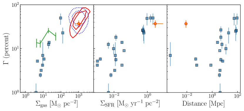
Figure 1: CFE as a function of gas surface density (left), star formation rate surface density (middle), and distance from the Sun (right). The CFE of Sgr B2 is indicated with an orange symbol; literature observations of the CFE in external galaxies are shown in blue. In the left-hand panel, the line indicates the observed CFE as a function of galactocentric radius in M83 (Adamo et al., 2015). The contours indicate the prediction of the Kruijssen (2012) model for Sgr B2 using the observed input parameters and their uncertainties listed in Table 3. Contours are shown at the 95% and 68% confidence levels for the local (blue) and global (red) renditions of the model. These panels demonstrate that there exist differences in the CFE even within our Galaxy, and that these differences are consistent with our theoretical understanding of bound cluster formation.

4 Conclusions

We have measured the cluster formation efficiency in the Galactic Center cloud Sgr B2, resulting in $\Gamma=37\pm 7\%$. This CFE is higher than that in the solar neighborhood, implying that the CFE varies within the Milky Way. Specifically, it changes with the galactic environment in a way that correlates with the local gas conditions. This observation is consistent with existing extragalactic observations. However, it additionally rules out the idea that the environmental dependence of the CFE is exclusively driven by an underlying dependence on the distance from the Sun, which affected previous work and would have been suggestive of an observational bias. Instead, our results show that the environmental variation of the CFE is a physical effect. The CFE model of Kruijssen (2012), in which higher average gas densities yield higher CFEs due to shorter free-fall times and higher star formation efficiencies, successfully predicts the observed value to within the uncertainties.

Table 3: Model parameters

Quantity	Units	Median	Uncertainty	‘Global model’	‘Local model’	Reference
$\log{\Sigma}$	[$\mathrm{M}_{\odot}~{}\mathrm{pc}^{-2}$]	3.00	0.22	✓		4
$\Omega$	[$\mathrm{Myr}^{-1}$]	1.80	0.25	✓		6,8
$\log{\rho}$	[$\mathrm{M}_{\odot}~{}\mathrm{pc}^{-3}$]	2.84	0.22		✓	9
$c_{\rm s}$	[$\textrm{km~{}s}^{-1}$]	0.53	0.07		✓	3,5
$\log{\sigma}$	[$\textrm{km~{}s}^{-1}$]	1.00	0.07	✓	✓	7
$\log{\Sigma_{\rm GMC}}$	[$\mathrm{M}_{\odot}~{}\mathrm{pc}^{-2}$]	3.61	0.18	✓	✓	2,10
$\log{\alpha_{\rm vir}}$	[–]	0.04	0.16	✓	✓	10
$\log{\beta_{0}}$	[–]	$-0.47$	0.32	✓	✓	1,2
$t_{\rm view}$	[$\mathrm{Myr}$]	0.74	0.16	✓	✓	6
$f_{\rm bound,global}$	[%]	44.8	13.1	✓		this work
$f_{\rm bound,local}$	[%]	48.9	11.6		✓	this work

Acknowledgements: We thank the anonymous referee for a timely and helpful report that led to substantial improvement of the paper. The National Radio Astronomy Observatory is a facility of the National Science Foundation operated under cooperative agreement by Associated Universities, Inc. This paper makes use of the following ALMA data: ADS/JAO.ALMA#2013.1.00269.S. ALMA is a partnership of ESO (representing its member states), NSF (USA) and NINS (Japan), together with NRC (Canada), NSC and ASIAA (Taiwan), and KASI (Republic of Korea), in cooperation with the Republic of Chile. The Joint ALMA Observatory is operated by ESO, AUI/NRAO and NAOJ. JMDK gratefully acknowledges funding from the German Research Foundation (DFG) in the form of an Emmy Noether Research Group (grant number KR4801/1-1), from the European Research Council (ERC) under the European Union’s Horizon 2020 research and innovation programme via the ERC Starting Grant MUSTANG (grant agreement number 714907), and from Sonderforschungsbereich SFB 881 “The Milky Way System” (subproject P1) of the DFG.

References

- Adamo et al. (2015) Adamo, A., Kruijssen, J. M. D., Bastian, N., Silva-Villa, E., & Ryon, J. 2015, MNRAS, 452, 246
- Adamo et al. (2013) Adamo, A., Östlin, G., Bastian, N., et al. 2013, ApJ, 766, 105
- Adamo et al. (2011) Adamo, A., Östlin, G., & Zackrisson, E. 2011, MNRAS, 417, 1904
- Alves et al. (2017) Alves, J., Lombardi, M., & Lada, C. J. 2017, A&A, 606, L2
- Barnes et al. (2017) Barnes, A. T., Longmore, S. N., Battersby, C., et al. 2017, MNRAS, 469, 2263
- Baumgardt & Kroupa (2007) Baumgardt, H., & Kroupa, P. 2007, MNRAS, 380, 1589
- Bigiel et al. (2008) Bigiel, F., Leroy, A., Walter, F., et al. 2008, AJ, 136, 2846
- Brodie & Strader (2006) Brodie, J. P., & Strader, J. 2006, ARA&A, 44, 193
- De Pree et al. (1996) De Pree, C. G., Gaume, R. A., Goss, W. M., & Claussen, M. J. 1996, ApJ, 464, 788
- De Pree et al. (2011) De Pree, C. G., Wilner, D. J., & Goss, W. M. 2011, AJ, 142, 177
- De Pree et al. (2015) De Pree, C. G., Peters, T., Mac Low, M. M., et al. 2015, ApJ, 815, 123
- Federrath et al. (2016) Federrath, C., Rathborne, J. M., Longmore, S. N., et al. 2016, ApJ, 832, 143
- Freeman et al. (2017) Freeman, P., Rosolowsky, E., Kruijssen, J. M. D., Bastian, N., & Adamo, A. 2017, MNRAS, 468, 1769
- Gaume et al. (1995) Gaume, R. A., Claussen, M. J., De Pree, C. G., Goss, W. M., & Mehringer, D. M. 1995, ApJ, 449, 663
- Ginsburg & Mirocha (2011) Ginsburg, A., & Mirocha, J. 2011, PySpecKit: Python Spectroscopic Toolkit, Astrophysics Source Code Library, , , ascl:1109.001
- Ginsburg et al. (2016a) Ginsburg, A., Goss, W. M., Goddi, C., et al. 2016a, A&A, 595, A27
- Ginsburg et al. (2016b) Ginsburg, A., Henkel, C., Ao, Y., et al. 2016b, A&A, 586, A50
- Ginsburg et al. (2018) Ginsburg, A., Bally, J., Barnes, A., et al. 2018, ApJ, 853, 171
- Henshaw et al. (2016) Henshaw, J. D., Longmore, S. N., & Kruijssen, J. M. D. 2016, MNRAS, 463, L122
- Hunter (2007) Hunter, J. D. 2007, Computing in Science and Engineering, 9, 90
- Johnson et al. (2016) Johnson, L. C., Seth, A. C., Dalcanton, J. J., et al. 2016, ApJ, 827, 33
- Kennicutt (1998) Kennicutt, Jr., R. C. 1998, ApJ, 498, 541
- Krieger et al. (2017) Krieger, N., Ott, J., Beuther, H., et al. 2017, ApJ, 850, 77
- Kroupa (2001) Kroupa, P. 2001, MNRAS, 322, 231
- Kruijssen (2012) Kruijssen, J. M. D. 2012, MNRAS, 426, 3008
- Kruijssen et al. (2015) Kruijssen, J. M. D., Dale, J. E., & Longmore, S. N. 2015, MNRAS, 447, 1059
- Kruijssen et al. (2012) Kruijssen, J. M. D., Maschberger, T., Moeckel, N., et al. 2012, MNRAS, 419, 841
- Kruijssen et al. (2018a) Kruijssen, J. M. D., Pfeffer, J. L., Reina-Campos, M., Crain, R. A., & Bastian, N. 2018a, MNRAS, arXiv:1806.05680
- Kruijssen et al. (2018b) Kruijssen, J. M. D., Schruba, A., Hygate, A. P. S., et al. 2018b, MNRAS, 479, 1866
- Kruijssen et al. (2018c) Kruijssen, J. M. D., Dale, J. E., Longmore, S. N., et al. 2018c, MNRAS-submitted
- Lada & Lada (2003) Lada, C. J., & Lada, E. A. 2003, ARA&A, 41, 57
- Launhardt et al. (2002) Launhardt, R., Zylka, R., & Mezger, P. G. 2002, A&A, 384, 112
- Leroy et al. (2013) Leroy, A. K., Walter, F., Sandstrom, K., et al. 2013, AJ, 146, 19
- Longmore et al. (2013) Longmore, S. N., Bally, J., Testi, L., et al. 2013, MNRAS, 429, 987
- Messa et al. (2018) Messa, M., Adamo, A., Calzetti, D., et al. 2018, MNRAS, 477, 1683
- Reina-Campos & Kruijssen (2017) Reina-Campos, M., & Kruijssen, J. M. D. 2017, MNRAS, 469, 1282
- Robitaille (2017) Robitaille, T. P. 2017, A&A, 600, A11
- Schmiedeke et al. (2016) Schmiedeke, A., Schilke, P., Möller, T., et al. 2016, A&A, 588, A143
- Walker et al. (2015) Walker, D. L., Longmore, S. N., Bastian, N., et al. 2015, MNRAS, 449, 715
- Zhang & Tan (2018) Zhang, Y., & Tan, J. C. 2018, ApJ, 853, 18