Energy-Momentum Distribution in General Relativity for a Phantom Black Hole Metric

Abstract

We use the Møller and Landau-Lifshitz energy-momentum definitions in General Relativity (GR) to evaluate the energy-momentum distribution of the phantom black hole space-time. The phantom black hole model was applied to the supermassive black hole at the Galactic Centre. We obtain that in both pseudotensorial prescriptions the energy distribution depends on the mass $M$ of the black hole, the phantom constant $p$ and the radial coordinate $r$. Further, all the calculated momenta are found to be zero. The limiting cases $r\rightarrow 0$, $r\rightarrow\infty$ and $r\rightarrow-\infty$ have also been the subject of the study.

1 Introduction

The energy-momentum localization is one of the most important subjects which remained unsolved in General Relativity (GR). Einstein was the first who calculated the energy-momentum complex in a general relativistic system Ein1915 . The conservation law for the energy-momentum tensor i.e. matter with non-gravitational fields for a physical system in (GR) is given by

$$\nabla_{\nu}T_{\mu}^{\nu}=0,$$ (1)

where $T_{\mu}^{\nu}$ is the symmetric energy-momentum tensor including the matter and non-gravitational fields. The energy-momentum complex $\tau_{\mu}^{\nu}$ satisfies a conservation law in the form of a divergence given by

$$\tau_{\mu,\nu}^{\nu}=0,$$ (2)

with

$$\tau_{\mu}^{\nu}=\sqrt{-g}(T_{\mu}^{\nu}+t_{\mu}^{\nu}),$$ (3)

where $g=\det g_{\nu\mu}$ and $t_{\mu}^{\nu}$ is the energy-momentum pseudotensor of the gravitational field. The energy-momentum complex can be written as

$$\tau_{\mu}^{\nu}=\theta_{\mu,\lambda}^{\nu\lambda},$$ (4)

with $\theta_{\mu}^{\nu\lambda}$ the superpotentials which are functions of the metric tensor and its first derivatives. From the above discussion the conclusion is that the energy-momentum complex is not uniquely defined. This is because one can add a quantity with an identically vanishing divergence to the expression $\tau_{\mu}^{\nu}$. Many famous physicists like Tolman Tolman , Landau and Lifshitz LL , Papapetrou Papapetrou , Bergmann BT and Weinberg Weinberg have given different definitions for the energy-momentum complexes. These expressions restricted the calculations of the energy distribution to quasi-Cartesian coordinates. Møller Moller introduced a new expression for the energy-momentum complex which is consistent and enables one to perform the calculations in any coordinate system. The Møller energy-momentum complex is significant for describing the energy-momentum in (GR). In this regard, we notice interesting results Many1 ; Many2 which recommend the Møller energy-momentum complex as an efficient tool for the energy-momentum localization. Furthermore, the other energy-momentum complexes are also important tools for the evaluation of the energy distribution and momentum of a given space-time and yielded meaningful physical results. In the context of the energy-momentum localization, it is very important to point out the agreement between the Einstein, Landau-Lifshitz, Papapetrou, Bergmann-Thomson, Weinberg and Møller definitions and the quasi-local mass definition introduced by Penrose Penrose and developed by Tod Tod for some gravitating systems. The energy-momentum localization in a Marder space-time has presented in Aygun/2007 . Further, the energy-momentum distributions of texture and monopole topological defects metrics in General Relativity are presented in Aygun/2010 .

In the early 90’s, Virabhadra revived the issue of energy-momentum localization by using different energy-momentum complexes in his pioneering works Many3 . Rosen Rosen employing the Einstein  prescription found that the total energy of the Friedman-Robertson-Walker (FRW) space-time is zero. Johri et al. Johri calculated the total energy of the (FRW) universe in the Landau-Lifshitz prescription and found that is zero at all times. The Einstein energy density for the Bianchi type-I space-time is also zero everywhere BS . Cooperstock and Israelit CI evaluated the energy distribution for a closed universe and found the zero value for a closed homogeneous isotropic( FRW) universe in (GR). Further,  to find an answer to the energy-momentum localization problem several scientists have used various energy-momentum complexes to evaluate the energy distribution for different space-times.

Moreover, recently the calculations performed for the $(3+1)$, $(2+1)$ and $(1+1)$ dimensional space-times have yielded physically reasonable results Many4 ; Many5 ; Many6 ; Many7 . We notice that several pseudotensorial prescriptions give the same results for any metric of the Kerr-Schild class JMA . Further, there is a similarity of some results with those obtained by using the teleparallel gravity Many8 . Working with the tetrad implies to encounter the notion of torsion, which can be used to describe (GR) entirely with respect to torsion instead of curvature derived from the metric only. This is called the teleparallel gravity equivalent to (GR). Energy-momentum complexes are quasi-local quantities associated with a closed 2-surface. Since Penrose introduced the definition of quasi-local mass Penrose , all the energy-momentum complexes present this property. The issue of energy localization is also correlated with the quasi-local energy given by Wang and Yau Wang/2009 . Searching for a common quasi-local energy value represents in fact the reabilitation of the pseudotensors. In this context, an important step has been made in the energy localization research by Chen et. al. Chen/2018 who discovered that with a 4D isometric Minkowski reference all of the quasi-local expressions in a large class give the same energy-momentum

In this paper we use the Møller and Landau-Lifshitz prescriptions to calculate the energy distribution for a metric that describes a phantom black hole. There are two basic reasons to apply the Møller energy momentum complex, the fact that it provides a powerful concept of energy and momentum in General Relativity (GR) and that the calculations are not restricted to quasi-Cartesian coordinates. Concerning the Landau-Lifshitz energy-momentum complex, this is also an useful tool to calculate the energy and momentum for a gravitating system and its use requires calculations to be made in quasi-Cartesian coordinates. In this study, for the Landau-Lifshitz prescription we have used the Schwarzschild Cartesian coordinates $\{t$, $x$, $y$, $z\}$ and in the case of the Møller prescription the Schwarzschild coordinates $\{t,$ $r,$ $\theta,$ $\phi\}$, respectively. The structure of the present paper is: in Section 2, we describe the phantom black hole Ding which is under study. Section 3 is focused on the presentation of the Møller energy-momentum complex and of the calculations of the energy distribution and momenta of the phantom black hole. In Section 4, we briefly introduce the Landau-Lifshitz energy-momentum complex and we evaluate the expressions for the energy and momenta. In Results and Discussion, we make a brief description of our results and present some limiting cases. The Conclusions section is devoted to the main conclusions of our study. In the paper, Greek (Latin) indices run from $0$ to $3$ ($1$ to $3$) and we use geometrized units, i.e. $c=G=1$.

2 Phantom Black Hole Metric

The observation of very distant supernovae made with the Hubble Space Telescope (HST) in 1998 indicated that the Universe is in an accelerated expansion. The Universe is made up of 68 % dark energy and the remaining about 30 % consists of dark matter and baryonic and nonbaryonic visible. Dark energy can be described with the aid of a phantom scalar field that represents a scalar with the minus sign for the kinetic term in the Lagrangian. Nowadays, cosmological models with phantom scalar fields have been extensively studied Many11 .

Furthermore, the phantom scalar field is of great interest in the physics of black holes. The Lagrangian is given by

$$L=\sqrt{-g}\biggl{[}-\frac{R}{8\pi G}+\epsilon g^{\mu\nu}\phi_{;\mu}\phi_{;\nu}-2V(\phi)\biggr{]}$$ (5)

The structure of the Lagrangian includes a scalar field, the potential $V(\phi)$ and $\epsilon$ that for the phantom takes the value $\epsilon=-1$.

A phantom black hole represents an exact solution of black holes in a phantom field. The Bronnikov-Fabris phantom black hole metric BF , later expressed by Ding et al. Ding is given by

$$ds^{2}=f(r)dt^{2}-\frac{dr^{2}}{f(r)}-(r^{2}+p^{2})(d\theta^{2}+\sin^{2}\theta d\phi^{2}),$$ (6)

with

$$f(r)=1-\frac{3M}{p}\biggl{[}\biggl{(}\frac{\pi}{2}-\arctan\frac{r}{p}\biggr{)}\biggl{(}1+\frac{r^{2}}{p^{2}}\biggr{)}-\frac{r}{p}\biggr{]},$$ (7)

where $M$ is the mass parameter and $p$ is a positive constant relative to the charge of phantom scalar fields known as the phantom constant Ding (here, $p$ is the phantom.) For the value $M=0$, Ding the metric describes the Ellis wormhole. The case $M<0$ corresponds to a wormhole which is asymptotically flat at $r\rightarrow\infty$ and has an anti-de Sitter bevaviour at $r\rightarrow-\infty$. For $M>0$ is obtained a regular black hole that presents a Schwarzschild-like causal structure at large distances $r$.

The potential is given by

$$\frac{\phi}{\sqrt{2}}=\psi=\arctan\frac{r}{p},\ \ V=\frac{3M}{p^{3}}\biggl{[}\bigg{(}\frac{\pi}{2}-\psi\bigg{)}(3-2\cos^{2}\psi)-3\sin\psi\cos\psi\biggr{]}.$$ (8)

The geometry of the phantom black hole can be used to obtain interesting information concerning dark energy effects on strong gravitational lensing, because the dark energy is modelled by the phantom scalar fields.

3 Møller Energy-Momentum Complex in GR and the Energy Distribution of the Phantom Black Hole

The energy-momentum complex of Møller Moller is given by

$$\mathcal{J}_{\nu}^{\mu}=\frac{1}{8\pi}\chi_{\nu\,\,,\,\lambda}^{\mu\lambda},$$ (9)

where the anti-symmetric superpotentials $\chi_{\nu}^{\mu\lambda}$ are

$$\chi_{\nu}^{\mu\lambda}=\sqrt{-g}\left(\frac{\partial g_{\nu\sigma}}{\partial x^{\kappa}}-\frac{\partial g_{\nu\kappa}}{\partial x^{\sigma}}\right)g^{\mu\kappa}g^{\lambda\sigma}$$ (10)

and satisfy the antisymmetric property

$$\chi_{\nu}^{\mu\lambda}=-\chi_{\nu}^{\lambda\mu}.$$ (11)

Møller’s energy-momentum complex, like other energy-momentum complexes satisfies the local conservation law

$$\frac{\partial\mathcal{J}_{\nu}^{\mu}}{\partial x^{\mu}}=0,$$ (12)

where $\mathcal{J}_{0}^{0}$ and $\mathcal{J}_{i}^{0}$ are the energy and the momentum densities, respectively. In the Møller definition, the energy-momentum is given by

$$P_{\nu}=\iiint\mathcal{J}_{\nu}^{0}dx^{1}dx^{2}dx^{3}.$$ (13)

The energy of the physical system has the following expression

$$E=\int\int\int\Im_{0}^{0}dx^{1}dx^{2}dx^{3}.$$ (14)

Further, using Gauss’s theorem, the energy $E$ can be written as

$$E=\frac{1}{8\pi}\int\int\chi_{0}^{0i}n_{i}dS,$$ (15)

where $n_{i}$ is the outward unit normal vector over an infinitesimal surface $dS$.
The expression of the determinant of the metric (6) is $g=-(r^{2}+p^{2})^{2}\sin^{2}\theta$. The non-vanishing covariant components of the metric (6) are

$$g_{00} = f(r),$$

$$g_{11} = -\frac{1}{f(r)},$$

$$g_{22} = -(r^{2}+p^{2}),$$

$$g_{33} = -(r^{2}+p^{2})\sin^{2}\theta.$$

The corresponding contravariant components of the metric tensor are given by

$$g^{00} = \frac{1}{f(r)},$$

$$g^{11} = -f(r),$$

$$g^{22} = \frac{-1}{(r^{2}+p^{2})},$$

$$g^{33} = \frac{-1}{(r^{2}+p^{2})\sin^{2}\theta},$$

For the line element (6) under consideration the only non-zero superpotential is given by

$$\chi_{0}^{01}=\frac{3M}{p}(r^{2}+p^{2})\biggl{[}\biggl{(}\arctan\frac{r}{p}-\frac{\pi}{2}\biggr{)}\frac{2r}{p^{2}}+\frac{2}{p}\biggr{]}\sin\theta.$$ (18)

Using the above expression and (15) we obtain the energy distribution of the phantom black hole

$$E_{M}(r)=\frac{3Mr^{2}}{2p}(r^{2}+p^{2})\biggl{[}\biggl{(}\arctan\frac{r}{p}-\frac{\pi}{2}\biggr{)}\frac{2r}{p^{2}}+\frac{2}{p}\biggr{]}.$$ (19)

Further, with (6) and (13) we found that all the momenta vanish

$$P_{r}=P_{\theta}=P_{\phi}=0.$$ (20)

We have plotted Fig. 1 and Fig. 2 to study the behaviour of the energy distribution $E_{M}(r)$  when increasing the radial distance $r$ and the phantom constant $p$. In both figures we have fixed the mass parameter $M$. From both graphical representations we notice that if $r\rightarrow 0$, $E_{M}(r)\rightarrow 0$  and when $r\rightarrow\infty$, $E_{M}(r)\rightarrow\infty$.

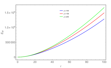
Figure 1: The energy $E_{M}$ vs. the radial distance $r$ for several values of phantom constant $p$ with $M=100$.

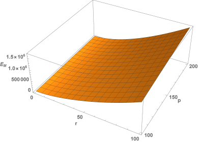
Figure 2: The 2-dimensional surface plot of the energy $E_{M}$. $E_{M}$ is plotted against the radial distance $r$ and the phantom constant $p$ with $M=100$.

In Fig. 3 and Fig. 4 we plot the energy $E_{M}$ near zero.

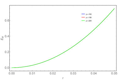
Figure 3: The energy $E_{M}$ vs. the radial distance $r$ for several values of phantom constant $p$ with $M=100$ near zero.

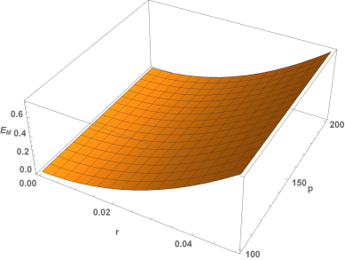
Figure 4: The 2-dimensional surface plot of the energy $E_{M}$. $E_{M}$ is plotted against the radial distance $r$ and the phantom constant $p$ with $M=100$ near zero.

4 Landau-Lifshitz Energy-Momentum Complex in GR and the Energy Distribution of the Phantom Black Hole

To perform the calculations of the energy distribution and momentum, the line element (6) is transformed to quasi-Cartesian coordinates $t,x,y,z$ using

$$x = r\sin\theta\cos\phi,$$

$$y = r\sin\theta\sin\phi,$$

$$z = r\cos\theta.$$ (21)

For the line element (6) we obtain the form

$$ds^{2} = f(r)dt^{2}-\frac{r^{2}+p^{2}}{r^{2}}(dx^{2}+dy^{2}+dz^{2})$$ (22)

$$-\biggl{(}\frac{1}{f(r)}-\frac{r^{2}+p^{2}}{r^{2}}\biggr{)}\biggl{(}\frac{xdx+ydy+zdz}{r}\biggr{)}^{2},$$

where

$$r=\sqrt{x^{2}+y^{2}+z^{2}}.$$ (23)

The generalized Landau-Lifshitz energy-momentum complex for GR theory is given by, LL

$$L^{\mu\nu}=\frac{1}{16\pi}S_{,\,\rho\sigma}^{\mu\nu\rho\sigma},$$ (24)

where the Landau-Lifshitz superpotentials are given by the expression

$$S^{\mu\nu\rho\sigma}=-g(g^{\mu\nu}g^{\rho\sigma}-g^{\mu\rho}g^{\nu\sigma}).$$ (25)

The $L^{00}$ and $L^{0i}$ components are the energy and the momentum densities, respectively. In the Landau-Lifshitz prescription the local conservation is respected

$$L_{,\,\nu}^{\mu\nu}=0.$$ (26)

By integrating $L^{\mu\nu}$ over the 3-space one gets the following expression for the energy and momentum

$$P^{\mu}=\iiint L^{\mu 0}\,dx^{1}dx^{2}dx^{3}.$$ (27)

By using Gauss’ theorem we obtain

$$P^{\mu}=\frac{1}{16\pi}\iint S_{,\nu}^{\mu 0i\nu}n_{i}dS=\frac{1}{16\pi}\iint U^{\mu 0i}n_{i}dS.$$ (28)

Using (24), (28) and the non-vanishining components of the Landau-Lifshitz superpotentials, we obtain the energy distribution of the phantom black hole

$$E_{LL}(r)=-\frac{\left(p^{2}+r^{2}\right)\left(6M\left(p^{4}-r^{4}\right)\tan^{-1}\left(\frac{r}{p}\right)-3\pi Mp^{4}+6Mp^{3}r-6Mpr^{3}+3\pi Mr^{4}+2p^{5}\right)}{2r^{3}\left(-6M\left(p^{2}+r^{2}\right)\tan^{-1}\left(\frac{r}{p}\right)+3\pi Mp^{2}-6Mpr+3\pi Mr^{2}-2p^{3}\right)}$$ (29)

In this prescription also all the momenta vanish.

$$P^{x}=P^{y}=P^{z}=0.$$

Fig. 5 and Fig. 6 show the dependence of the energy $E_{LL}$ on the radial distance $r$ and phantom parameter $p$ for a constant value of the mass $M$ of the phantom black hole.

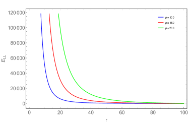
Figure 5: The energy $E_{LL}$ vs. the radial distance $r$ for several values of phantom constant $p$ with $M=100$.

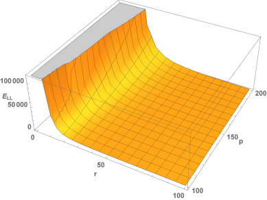
Figure 6: The 2-dimensional surface plot of the energy $E_{LL}$. $E_{LL}$ is plotted against the radial distance $r$ and the phantom constant $p$ with $M=100$.

The behaviour of the energy near zero is presented in Fig. 7 and Fig. 8.

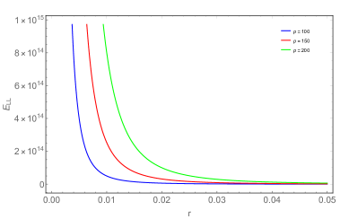
Figure 7: The energy $E_{LL}$ vs. the radial distance $r$ for several values of phantom constant $p$ with $M=100$ near zero.

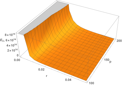
Figure 8: The 2-dimensional surface plot of the energy $E_{LL}$. $E_{LL}$ is plotted against the radial distance $r$ and the phantom constant $p$ with $M=100$ near zero.

5 Results and Discussion

The energy-momentum complexes provide the same energy-momentum distribution for many gravitating systems. However, for some space-times the results obtained with various prescriptions differ each other. Hence, the debate on the localization of energy  is one of the most actual and interesting problem in (GR). The study of the energy-momentum distribution can also give a clear idea about the space-time. One can study the gravitational lensing of the spacetime analyzing the energy. Virbhadra VirEllisLens derived interesting lensing phenomena using the analysis of the energy distribution in curved space-time. We also point out some meaningful results obtained by the authors with the pseudotensorial prescriptions, and in this view we draw attention to some research papers elaborated in the last two decades on this issue Radinschi/2001 ; Radinschi/2007 ; Radinschi/2010 ; Radinschi/2011 ; sahoo/2015 ; Radinschi/2016 .

In this paper we calculated the energy distribution of the phantom black hole using the Møller and Landau-Lifshitz energy-momentum complexes. In both prescriptions the energy distribution depends on the mass $M$ of the black hole, the phantom constant $p$ and the radial coordinate $r$. $E_{M}(r)$ and $E_{LL}(r)$ represent the total (matter plus gravitational field) energy within radius $r$ in the Møller and Landau-Lifshitz prescriptions, respectively. From the calculations, it results that in these prescriptions all the momenta are zero. The expressions of the energy distribution obtained in these two prescriptions are different because of the differences between the superpotentials which constitute the Møller and Landau-Lifshitz energy-momentum complexes, as well as by the structure of the studied metric. Furthermore, the difference in the order of magnitude for the energy calculated in both prescriptions is due to different expressions of the Møller and Landau-Lifshitz energy-momentum complexes.

A clarification and a physical interpretation of the results obtained with the Møller and Landau-Lifshitz energy-momentum complexes is now needed. To calculate the energy-momentum distributions it is important, because we can obtain useful information about the gravitational background like the value of the effective gravitational mass of the source of spacetime curvature, and also a prediction about the gravitational lensing. The positive energy distribution region plays the role of a convergent lens and the negative one serves as a divergent lens.

A limiting case that is of special interest is the behaviour of the energy near the origin, that is for $r\rightarrow 0$. For some spacetimes here the metric goes infinite, a singularity arises and the energy distribution and momentum deal with extreme values. This behavior is in connection with the spacetime geometry. We expect that the expression of the energy distribution will give us some details about the utility of the applied energy-momentum complex. In the case of the Møller energy-momentum complex we found that for $r\rightarrow 0$ the energy tends to zero. For the Landau-Lifshitz energy momentum-complex for $r\rightarrow 0$ the energy tends to plus infinity.

Also, the results obtained in this work exhibit that there is no finite value for the energy when $r\rightarrow\infty$. One can compare these results with our previous result sahoo/2015 obtained with the Einstein energy momentum complex for the same metric. In our previous paper the energy distribution is positive and becomes constant for increasing the radial distance $r$. In the present work, for increasing the radial distance the energy distribution becomes infinite for larger values of $r$ in the case of the Møller prescription and tends to minus infinity in the case of the Landau-Lifshitz prescription. The energy distribution calculated in the Møller prescription takes only positive values for any values of the parameters $p$ and $M$. Furthermore, from our study we have detected that the energy distribution in the Landau-Lifshitz prescription has both positive and negative values for some preferred values of the parameters $p$ and $M$. These results come to support the use of the Møller and Landau-Lifshitz energy-momentum complexes for the evaluation of the energy-distribution of a given space-time, because the positive energy region serves as a convergent lens and the negative one as a divergent lens Virbhadra/2000 .

The limiting cases $r\rightarrow 0$, $r\rightarrow\infty$ and $r\rightarrow-\infty$ are presented in Table 1.

Table 1:

Energy	$r\rightarrow 0$	$r\rightarrow\infty$	$r\rightarrow-\infty$
$E_{M}$	$0$	$\infty$	$\infty$
$E_{LL}$	$\infty$	$-\infty$	$\infty$

The phantom scalar could play an important role in black hole physics and it would be of interest to test this phantom field, the best approach being gravitational lensing. Microlensing is useful to probe dark matter and dark energy in the Galatic halo Chang/1979 . For the metric given by (6) for a small value of the phantom $p$ or in the case $p\rightarrow 0$ the phantom black hole behaves as a so called Schwarzschild phantom black hole, and the single event horizon is $r_{+}=2\,M$. If $p$ increases, the radius of the event horizon decreases and a stronger effect from dark energy is noticeable.The phantom $p$ has a behaviour similar to the electric charge in the Reissner-Nordström black hole allowing the comparison between the phantom black hole lensing and the Reissner-Nordström lensing. So, the metric described by (6) can yield useful information about dark energy effects on strong gravitational lensing. Very interesting is the behaviour of the energy distribution in the Møller and Landau-Lifshitz prescriptions near the event horizon. As we pointed out, the positive and negative regions of the energy serve as convergent and divergent lenses, respectively. Both expressions of the energy distribution $E_{M}(r)$ and $E_{LL}(r)$ contain the phantom $p$ and this could have effects on strong gravitational lensing. To study the behaviour of the energy distribution near the event horizon we performed a Taylor expansion of $E_{M}(r)$ and $E_{LL}(r)$ in function of $r=2\,M$ in the particular case $p=150$ and $M=100$, and we plot these expressions for $r=2\,M$ in Fig. 9 and Fig. 10, respectively. As we expected, the energy in the Møller prescription near the event horizon $E_{HM}$ takes only positive values and plays the role of a convergent lens. In the case of the Landau-Lifshitz prescription, the energy near the event horizon $E_{HLL\text{ }}$takes both positive and negative values and serves as a convergent and divergent lens, respectively. Obviously, a deeper study of the effects of dark energy on the strong gravitational lensing in the case of the phantom black hole is required.

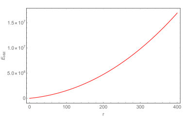
Figure 9: The energy $E_{HM}$ near event horizon vs. the radial distance $r$ with $p=150$ and $M=100$.

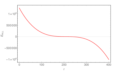
Figure 10: The energy $E_{HLL}$ near event horizon vs. the radial distance $r$ with $p=150$ and $M=100$.

As stated by the results obtained in this work and in our previous work sahoo/2015 we can conclude that the Einstein and Møller prescriptions are useful tools for the localization of energy.

6 Conclusions

The Landau-Lifshitz energy-momentum complex presents some singularities that are determined by the metric structure. One of these singularities is $r\rightarrow 0$ which appears for any values of the phantom parameter $p$ and mass $M$ of the phantom black hole. The other singularities are the roots of the second degree equation $6\arctan\bigl{(}\frac{r}{p}\bigr{)}p^{2}M+6\arctan\bigl{(}\frac{r}{p}\bigr{)}Mr^{2}+2p^{3}-3p^{2}M\pi+6pMr-3M\pi r^{2}=0$.

As a conclusion, even it also yields positive values for the energy distribution and gives physically acceptable results, the Landau-Lifshitz energy-momentum complex is not the most suitable tool for the the energy-momentum localization in the case of the phantom black hole. An interesting future work lies in the calculation of the energy with the aid of other energy-momentum complexes and the teleparallel equivalent to (GR).

Acknowledgements PKS acknowledges DST, New Delhi, India for providing facilities through DST-FIST lab, Department of Mathematics, where a part of this work was done. The authors also thank the referee for the valuable suggestions, which improved the presentation of the obtained results.

References

- (1) A Einstein Preuss. Akad. Wiss. Berlin 47 844 (1915)
- (2) R C Tolman Phys. Rev. 35 875 (1930)
- (3) L D Landau, E M Lifshitz The Classical Theory of Fields (Pergamon Press) p 280 (1987)
- (4) A Papapetrou Proc. R. Irish. Acad. A52 11 (1948)
- (5) P G Bergmann, R Thomson Phys. Rev. 89 400 (1953)
- (6) S Weinberg Gravitation and Cosmology: Principles and Applications of General Theory of Relativity (John Wiley and Sons, Inc., New York) p 165 (1972)
- (7) C Møller Ann. Phys. (NY) 4 347 (1958); 12 118 (1961)
- (8) S S Xulu Mod. Phys. Lett. A 15 1511 (2000); Ph. D. Thesis, hep-th/0308070; Astrophys. Space Sci. 283 23 (2003); E C Vagenas Mod. Phys. Lett. A 19 213 (2004); R Gad Astrophys. Space Sci. 295 459 (2005); M Sharif, Tasnim Fatima Nuovo Cim. B120 533 (2005); I-Ching Yang Chin. J. Phys. 45 497 (2006); S H Mehdipour Astrophys. Space Sci. 352 877 (2014)
- (9) I Radinschi Fizika B 9 203 (2000); Mod. Phys. Lett. A 15 2171 (2000); Chin. J. Phys. 39 231 (2001); Mod. Phys. Lett. A 16 673 (2001)
- (10) R Penrose Proc. R. Soc. London A381 53 (1982)
- (11) K P Tod Proc. R. Soc. London A388 457 (1983)
- (12) S. Aygũn, M. Aygũn, I. Tarhan Pramana - J Phys 68 21 (2007)
- (13) S. Aygũn, Int. J. Theor. Phys. 49 2288 (2010)
- (14) K S Virbhadra Phys. Rev. D 41 1086 (1990); ibid 42 1066 (1990); ibid 42 2919 (1990); ibid 60 104041 (1999); Phys. Lett. A 157 195 (1991); Pramana 38, 31 (1992); N Rosen, K S Virbhadra Gen. Relativ. Gravit. 25 429 (1993); K S Virbhadra, J C Parikh Phys. Lett. B 317 312 (1993); ibid 331 302 (1994); K S Virbhadra Pramana 45 215 (1995); A Chamorro, K S Virbhadra Pramana-J. Phys. 45 181 (1995); Int. J. Mod. Phys. D 5 251 (1996); K S Virbhadra Int. J. Mod. Phys. A 12 4831 (1997); ibid D 6 357 (1997)
- (15) N Rosen Gen. Relativ. Gravit. 27 313 (1995)
- (16) V B Johri et al. Gen. Relat. Grav. 27, 313 (1995)
- (17) N Banerjee, S Sen Pramana 49 609 (1997)
- (18) F I Cooperstock, M Israelit Found. Phys. 25 631 (1995)
- (19) S S Xulu Int. J. Mod. Phys. A 15 2979 (2000); S S Xulu Int. J. Theor. Phys. 39 1153 (2000); M Sharif, M Azam Int. J. Mod. Physi. A 22 1935 (2007); I -C Yang, I Radinschi Chin. J. Phys. 42 40 (2004); A K Sihna et al. Mod. Phys. Lett. A 30 1550120 (2015); S K Tripathy et al. Adv. High Energy Phys. 2015 705262 (2015); Prajyot Kumar Mishra et al. Adv. High Energy Phys. 2016 1986387 (2016)
- (20) E C Vagenas Int. J. Mod. Phys. A 18 5781 (2003); E C Vagenas Int. J. Mod. Phys. A 18 5949 (2003); E C Vagenas Mod. Phys. Lett. A 19 213 (2004); S S Xulu Int. J. Mod. Phy. D 13 1019 (2004); S S Xulu Chin. J. Phys. 44, 348 (2006); S S Xulu Found. Phys. Lett. 19 603 (2006); S S Xulu Int. J. Theor. Phys. 46 2915 (2007)
- (21) S L Loi, T Vargas Chin. J. Phys. 43 901 (2005)
- (22) E C Vagenas Int. J. Mod. Phy. D 14 573 (2005); E C Vagenas Mod. Phys. Lett. A 21 1947 (2006); T Multamaki, A Putaja, E C Vagenas, I Vija Class. Quant. Grav. 25 075017 (2008); Amir M Abbassi, Saeed Mirshekari, Amir H. Abbasssi Phys. Rev. D 78 064053 (2008); M Abdel-Megied, Ragab M. Gad Adv. High Energy Phys. 2010 379473 (2010); Irina Radinschi, Theophanes Grammenos, Andromahi Spanou Centr. Eur. J. Phys. 9 1173 (2011); I-Ching Yang Chin. J. Phys. 50 544 (2012); I-Ching Yang, Bai-An Chen, Chung-Chin Tsai Mod. Phys. Lett. A 27 1250169 (2012); Ragab M Gad Astrophys. Space Sci. 346 553 (2013); M Saleh, B.B. Thomas, T C Kofane Commun. Theor. Phys. 55 291 (2011); Mahamat Saleh, Bouetou Bouetou Thomas, Kofane Timoleon Crepin Chin. Phys. Lett. 34 080401 (2017) I Radinschi, Th. Grammenos, F Rahaman, A Spanou, S Islam, S Chattopadhyay, A Pasqua Adv. High Energy Phys. 2017 7656389 (2017).
- (23) J M Agurregabiria, A. Chamorro, K S Virabhadra Gen. Relat. Grav. 28 1393 (1996)
- (24) Gamal G L Nashed Phys. Rev. D 66 064015 (2002); Mod. Phys. Lett. A 22 1047 (2007); S. Aygũn, H. Baysal, I. Tarhan, Int. J. Theor. Phys. 46 2607 (2007); Gamal G L Nashed, T Shirafuji Int. J. Mod. Phys. D16 65 (2007); Int. J. Mod. Phys. A 23 1903 (2008); Gamal G L Nashed Chin. Phys. B19(2) 020401 (2010); M Sharif, Abdul Jawad Astrophys. Space Sci. 331 257 (2011); Gamal G L Nashed Adv. High Energy Phys. 2012 475460 (2012); Gamal G L Nashed Int. J. Theor. Phys. 53 1654 (2014); S Aygũn, H Baysal, Can Aktas, I Yilmaz, P. K. Sahoo, I Tarhan Int. J. Mod. Phys. A 33 1850184 (2018); M G Ganiou, M J S Houndjo, J Tossa Int. J. Mod. Phy. D 27 1850039 (2018); M. F. Mourad Indian J Phys 93, 1233 (2019).
- (25) M -T Wang, S -T Yau Phys. Rev. Lett. 102 021101 (2009); Commun. Math. Phys. 288, 919 (2009).
- (26) Chiang-Mei Chen, Jian-Liang Liu, James M Nester Int. J. Mod. Phys. D 27 1847017 (2018); Chiang-Mei Chen, Jian-Liang Liu, James M Nester Gen. Relativ. Gravit. 50 158 (2018)
- (27) C Ding, C Liu, Y Xiao, L Jiang, R G Cai, Phys. Rev. D 88 104007 (2013)
- (28) L P Chimento, R Lazkoz Phys. Rev. Lett. 91 211301 (2003); R R Caldwell, M Kamionkowski, N N Weinberg Phys. Rev. Lett. 91 071301 (2003); A Vikman Phys. Rev. D 71 023515 (2005); Z Y Sun, Y G Shen Gen. Rel. Grav. 37 243 (2005); R Gannouji, D Polarski, A Ranquet, A A Starobinsky JCAP 0609 016 (2006); S Chattopadhyay, U Debnath Braz. J. Phys. 39 86 (2009)
- (29) K A Bronnikov, J C Fabris, Phys. Rev. Lett. 96 251101 (2006)
- (30) K S Virbhadra, D. Narasimha, S M Chitre Astron. Astrophys. 337 1 (1998); K S Virbhadra, G F R Ellis Phys. Rev. D 62 084003 (2000); C -M Claudel, K S Virbhadra, G F R Ellis J. Math. Phys. 42 818 (2001); K S Virbhadra, G F R Ellis Phys. Rev. D 65 103004 (2002); K S Virbhadra, C.R. Keeton Phys. Rev. D 77 124014 (2008); K S Virbhadra Phys. Rev. D 79 083004 (2009)
- (31) I Radinschi, Chin. J. Phys. 39(5) 393 (2001)
- (32) Th. Grammenos, I. Radinschi, Int. J. Theor. Phys. 46(4) 1055, (2007)
- (33) I Radinschi, F Rahaman, A Gosh, Int. J. Theor. Phys. 49(5) 943 (2010)
- (34) I Radinschi, F Rahaman, A Banerjee, Int. J. Theor. Phys. 50(9) 2906, (2011)
- (35) P K Sahoo et al. Chin. Phys. Lett. 32 020402 (2015)
- (36) I Radinschi et al., Adv. High Energy Phys., 2016 9049308 (2016)
- (37) K S Virbhadra, George F R Ellis Phys. Rev. D 62 084003 (2000)
- (38) K. Chang, S. Refsdal, Nature (London) 282 561 (1979)